eqs

$$\begin{split}\BODY\end{split}$$ (1)

Abstract

Utilizing the framework of $\mathbb{Z}_{2}$ lattice gauge theories in the context of Pauli stabilizer codes, we present methodologies for simulating fermions via qubit systems on a two-dimensional square lattice. We investigate the symplectic automorphisms of the Pauli module over the Laurent polynomial ring. This enables us to systematically increase the code distances of stabilizer codes while fixing the rate between encoded logical fermions and physical qubits. We identify a family of stabilizer codes suitable for fermion simulation, achieving code distances of $d=2,3,4,5,6,7$, allowing correction of any $\lfloor\frac{d-1}{2}\rfloor$-qubit error. In contrast to the traditional code concatenation approach, our method can increase the code distances without decreasing the (fermionic) code rate. In particular, we explicitly show all stabilizers and logical operators for codes with code distances of $d=3,4,5$. We provide syndromes for all Pauli errors and invent a syndrome-matching algorithm to compute code distances numerically.

 

Contents

1. 1 Introduction
2. 2 Results
   1. 2.1 Review of the original bosonization
   2. 2.2 Bosonization with code distance $d=3$
   3. 2.3 Bosonization with code distance $d=4$
   4. 2.4 Bosonization with code distance $d=5$
3. 3 Stabilizer codes and the Pauli module
   1. 3.1 Review of the Laurent polynomial method for the Pauli algebra
   2. 3.2 New stabilizer codes developed from automorphisms
      1. 3.2.1 Automorphism for code distance $d=3$

 

1 Introduction

Error-correcting codes were initially developed to correct quantum errors on noisy quantum devices and have found further applications in condensed matter physics and high-energy physics. The cornerstone of quantum error correction is the stabilizer formalism [gottesman1997stabilizer], which defines the codewords in the common eigenspace of elements in an Abelian group, referred to as the stabilizer group. A stabilizer code is labeled $[[n,k,d]]$ when it uses $n$ physical qubits to encode $k$ logical qubits with code distance $d$. The code distance is the minimum weight of an operator that commutes with all elements in the stabilizer group but is not in the stabilizer group itself. The ratios $\frac{k}{n}$ and $\frac{d}{n}$ determine the quality of codes. Recent developments show the existence of “good” quantum low-density parity-check (LDPC) codes, i.e., with the number of logical qubits $k$ and the code distance $d$ both scaling linearly with the number of physical qubits $n$ [PK22_1, PK22_2, lin2022good, dinur2023good]. In this paper, our focus is on a different objective. Instead of encoding logical qubits, we aim to encode logical fermions using physical qubits. This motivation comes from the need to simulate fermions on quantum computers since most models of matter involve electrons, which are, in fact, fermions [jordan1993paulische, fradkin89jordan, BK02, barends2015digital, hensgens2017quantum, mazurenko2017cold, tarruell2019quantum, Google_Fermi_2020, hebbe2021benchmarking]. While fault-tolerant quantum computation [toric_code_2003, Surface_codes_2012] is the ultimate goal, current devices still have limited resources and suffer from noise, so error-mitigation schemes are crucial. Therefore, we seek an effective design such that when we implement fermions with qubits on a quantum computer, certain physical qubit errors can be corrected directly in this protocol without having to encode the underlying qubits further. Thus, we want to systematically increase the code distance $d$ in a fermion-to-qubit mapping with a fixed code rate (between logical fermions and physical qubits).

When a fermionic Hamiltonian consists of geometrically local terms, they can be mapped to local qubit operators by the Bravyi-Kitaev superfast encoding and its variants [BK02, Setia19superfast], by the auxiliary methods [B05, VC05, WH16, MS_auxiliary, compact_mapping, po2021symmetric], or by exact bosonization [CKR18, CK19, C20]. The mappings between fermionic Hamiltonians and higher-spin Hamiltonians are also studied in Refs. [wosiek1981local, Ruba_constraints_2020, Ruba_bosonization_2020, Ruba_bosonization_2022]. There are also proposals that utilize defects of surface codes for fermionic quantum simulation [bombin2010topo, hastings2014reduced, brown2017poking], and those defects are recently implemented by Google Quantum AI [google2023non]. Variants of these mappings have been studied to optimize different costs [Mark_varying_resource_2018, Steudtner_Quantum_codes2019, chien2020custom, jiang2020optimal, bausch2020mitigating, chiew2021optimal, derby2021compact, landahl2021logical, harrison2022reducing, o2022ultrafast, Zheng2022Boson_fermion_duality, li2022unified, algaba2023lowdepth, equivalence_CX]. In the context of quantum many-body physics, these mappings also reveal the deep connections between fermion and spin systems [kitaev2006anyons, wen2003quantum]. There is another exact fermion-flux lattice duality derived from the $\mathbb{Z}_{2}$ gauge theory [chen2022berry]. Aside from the investigation of constructing new mappings, fermion-to-qubit mappings have been studied in the context of variational quantum circuits [nys2022variational, nys2023quantum]. In all the above-mentioned methods, extra qubits are required, e.g., the number of qubits is twice the number of fermions on a 2d square lattice. This is the price for the locality-preserving property. These methods can be thought of as stabilizer codes. Given $N$ fermions with the Hilbert space dimension $2^{N}$, they are mapped to $2N$ qubits with space dimension $2^{2N}$, which is an enlarged space. After $N$ gauge constraints (stabilizer conditions) are imposed, the gauge-invariant subspace (code space) has dimension $2^{N}$, which matches the dimension of the logical fermions. It has been shown that gauge constraints can be utilized for error correction [Wiebe_2021_quantum], and code distances can be studied for these stabilizer codes. Ref. [Setia19superfast] demonstrates that an improved Bravyi-Kitaev superfast encoding can correct any single-qubit error in a graph where each vertex has degree $d\geq 6$. In Ref. [MLSC_2019], another version of the Bravyi-Kitaev superfast encoding is proposed, called the “Majorana loop stabilizer code,” which is designed to have code distance $d=3$ such that any single-qubit error can be corrected. However, it is not known how to generalize the Bravyi-Kitaev superfast encoding to produce codes with higher and higher code distances. An alternative approach is code concatenation, where logical qubits in error-correcting codes replace physical qubits in the fermion-to-qubit mappings. However, code concatenation will decrease the code rate between logical fermions and physical qubits, increasing the overhead of fermionic simulation. In this work, we present a method that increases the code distances of the fermion-to-qubit mappings while preserving the code rate.

In this paper, we conjugate an existing stabilizer code with a Clifford circuit. This produces a new stabilizer code. Since the new code is obtained via conjugation by a unitary operator, the algebra of the logical operators is preserved. If we choose the circuit wisely, the new stabilizer code will have a larger code distance $(d\geq 3)$, compared to the code distance $d=2$ of the original exact bosonization. To study Clifford circuits systematically, we utilize the Laurent polynomial method introduced in Refs. [Haah_module_13, Haah_2016] and further extended in Ref. [Ruba_Yang], which shows that any Pauli operator can be written as a vector in a symplectic space. For a system with translational symmetry, e.g., the 2d square lattice, the space of Pauli operators becomes a module over a polynomial ring. Furthermore, this polynomial method can be used to formulate the 2d bosonization concisely [Nat_JW_2020]. The commutation relations of Pauli operators are determined by the symplectic form. Ref. [haah2021clifford] shows that there is a one-to-one correspondence (up to a translation operator on the lattice): Automorphism of the symplectic form ⟺Clifford circuit on a 2d square lattice. Therefore, the problem of finding new codes turns into a problem of searching for “good” automorphisms of the Pauli module with the symplectic form, which can be achieved efficiently by exhaustive numerical search.

	distance	occupation	hopping	interaction	stabilizer
Bravyi-Kitaev superfast encoding	2	4	6	6	6
Majorana loop stabilizer code	3	3	3-4	4-6	4-10
Exact bosonization ($d=3$)	3	4	3-5	6	8
Exact bosonization ($d=4$)	4	6	5-6	10	10
Exact bosonization ($d=5$)	5	8	5-9	12-14	12
Exact bosonization ($d=6$)	6	12	6-13	16-20	18
Exact bosonization ($d=7$)	7	12	7-23	16-18	26

Table 1: A comparison of codes based on modified exact bosonization to the Bravyi-Kitaev superfast encoding [BK02] and to the Majorana loop stabilizer code [MLSC_2019] on a 2d square lattice. The $d=2$ exact bosonization is equivalent to the Bravyi-Kitaev superfast encoding with a specific choice of the ordering of edges [equivalence_CX]. We list the code distance, as well as the weights (after mapping to qubits) of a fermion occupation term (local fermion parity term), of a hopping term, and of a density-density interaction between nearest neighbors. The weights of the stabilizers are also shown.

In this work, we use the Laurent polynomial method to construct bosonizations on a 2d square lattice. Table 1 is the summary of our results. In Section 2, we review the original 2d bosonization method [CKR18] in Section 2.1 and then pictorially construct 2d bosonizations with distances of $3,4$, and $5$ in Section 2.2, 2.3, and 2.4, respectively. We review the Laurent polynomial method in Section. 3.1. In Section. 3.2, we describe all these bosonizations within the framework of the Laurent polynomial method. In addition, in Section. LABEL:sec:bosonization_search, we describe a computerized method to search for bosonizations. In Appendix LABEL:sec:_syndrome_matching_method, we discuss the “syndrome matching” method used to compute the code distance of a given bosonization. In Appendix LABEL:sec:_elementary_automorphism, we describe the generators of the symplectic group and choose sixteen elementary automorphisms for our numerical search algorithm. In Appendix LABEL:sec:polynomial_d=6,7, we show the polynomial representations of an automorphism with a distance of 6 and another with a distance of 7.

2 Results

In Section 2.1, we begin by reviewing the original 2d bosonization on a square lattice from Ref. [CKR18]. Then we demonstrate a new way to perform bosonization with code distances of $d=3$, $d=4$, and $d=5$ in Section 2.2, Section 2.3, and Section 2.4, respectively.

2.1 Review of the original bosonization

Figure 1: Bosonization on a square lattice [CKR18]. We put Pauli matrices $X_{e}$, $Y_{e}$, and $Z_{e}$ on each edge and one complex fermion $c_{f},c_{f}^{\dagger}$ on each face. We will work in the Majorana basis $\gamma_{f}=c_{f}+c_{f}^{\dagger}$ and $\gamma^{\prime}_{f}=-i(c_{f}-c_{f}^{\dagger})$ for convenience.

We first describe the Hilbert space in Fig. 1. The elements associated with vertices, edges, and faces will be denoted by $v$, $e$, and $f$, respectively. On each face $f$ of the lattice, we place a single pair of fermionic creation-annihilation operators $c_{f},c_{f}^{\dagger}$, or equivalently a pair of Majorana fermions $\gamma_{f},\gamma^{\prime}_{f}$. The even fermionic algebra consists of local observables with trivial fermionic parity, i.e., local observables that commute with the total fermion parity $(-1)^{F}\equiv\prod_{f}(-1)^{c^{\dagger}_{f}c_{f}}$ where $F=\sum_{f}c^{\dagger}_{f}c_{f}$ is the total fermion number. The even algebra is generated by [CKR18]:

1. On-site fermion parity (occupation):

   $$P_{f}\equiv-i\gamma_{f}\gamma^{\prime}_{f}.$$ (2)

2. Fermionic hopping term:

   $$S_{e}\equiv i\gamma_{L(e)}\gamma^{\prime}_{R(e)},$$ (3)

   where $L(e)$ and $R(e)$ are faces to the left and right of $e$, with respect to the orientation of $e$ in Fig. 1.

The bosonic dual of this system involves ${\mathbb{Z}}_{2}$-valued spins on the edges of the square lattice. For every edge $e$, we define a unitary operator $U_{e}$ that squares to $1$. Labeling the faces and vertices as in Fig. 1, we define:

$$\begin{split}U_{56}&=X_{56}Z_{25},\\ U_{58}&=X_{58}Z_{45},\end{split}$$ (4)

where $X_{e}$, $Z_{e}$ are Pauli matrices acting on a spin at edge $e$:

$$X_{e}=\begin{bmatrix}0&1\\ 1&0\end{bmatrix},~{}Z_{e}=\begin{bmatrix}1&0\\ 0&-1\end{bmatrix}.$$ (5)

Operators $U_{e}$ for the other edges are defined by using translation symmetry. Pictorially, operator $U_{e}$ is depicted as

$$U_{e}=\begin{gathered}\lx@xy@svg{\hbox{\raise 0.0pt\hbox{\kern 3.0pt\hbox{\ignorespaces\ignorespaces\ignorespaces\hbox{\vtop{\kern 0.0pt\offinterlineskip\halign{\entry@#!@&&\entry@@#!@\cr&\\&\crcr}}}\ignorespaces{\hbox{\kern-3.0pt\raise 0.0pt\hbox{\hbox{\kern 0.0pt\raise 0.0pt\hbox{\hbox{\kern 3.0pt\raise 0.0pt\hbox{$\textstyle{}$}}}}}}}{\hbox{\kern 31.45274pt\raise 0.0pt\hbox{\hbox{\kern 0.0pt\raise 0.0pt\hbox{\hbox{\kern 3.0pt\raise 0.0pt\hbox{$\textstyle{{}\ignorespaces\ignorespaces\ignorespaces\ignorespaces\ignorespaces}$}}}}}}}\ignorespaces\ignorespaces\ignorespaces\ignorespaces{}{\hbox{\lx@xy@droprule}}\ignorespaces{\hbox{\kern 28.61427pt\raise-17.22636pt\hbox{\hbox{\kern 0.0pt\raise-2.81389pt\hbox{$\scriptstyle{\displaystyle X_{e}}$}}}}}{\hbox{\lx@xy@droprule}}\ignorespaces{}{\hbox{\lx@xy@droprule}}{\hbox{\lx@xy@droprule}}{\hbox{\kern-3.0pt\raise-34.45274pt\hbox{\hbox{\kern 0.0pt\raise 0.0pt\hbox{\hbox{\kern 3.0pt\raise 0.0pt\hbox{$\textstyle{{}\ignorespaces\ignorespaces\ignorespaces\ignorespaces\ignorespaces}$}}}}}}}\ignorespaces\ignorespaces\ignorespaces\ignorespaces{}{\hbox{\lx@xy@droprule}}\ignorespaces{\hbox{\kern 13.45554pt\raise-34.45274pt\hbox{\hbox{\kern 0.0pt\raise-3.41666pt\hbox{$\scriptstyle{\displaystyle Z}$}}}}}{\hbox{\lx@xy@droprule}}\ignorespaces{}{\hbox{\lx@xy@droprule}}{\hbox{\lx@xy@droprule}}{\hbox{\kern 31.45274pt\raise-34.45274pt\hbox{\hbox{\kern 0.0pt\raise 0.0pt\hbox{\hbox{\kern 3.0pt\raise 0.0pt\hbox{$\textstyle{}$}}}}}}}\ignorespaces}}}}\ignorespaces\end{gathered}\qquad\text{or}\qquad\begin{gathered}\lx@xy@svg{\hbox{\raise 0.0pt\hbox{\kern 3.77083pt\hbox{\ignorespaces\ignorespaces\ignorespaces\hbox{\vtop{\kern 0.0pt\offinterlineskip\halign{\entry@#!@&&\entry@@#!@\cr&\\&\crcr}}}\ignorespaces{\hbox{\kern-3.0pt\raise 0.0pt\hbox{\hbox{\kern 0.0pt\raise 0.0pt\hbox{\hbox{\kern 3.0pt\raise 0.0pt\hbox{$\textstyle{{}\ignorespaces\ignorespaces\ignorespaces\ignorespaces\ignorespaces}$}}}}}}}\ignorespaces\ignorespaces\ignorespaces\ignorespaces{}{\hbox{\lx@xy@droprule}}\ignorespaces{\hbox{\kern 11.3879pt\raise 0.0pt\hbox{\hbox{\kern 0.0pt\raise-2.81389pt\hbox{$\scriptstyle{\displaystyle X_{e}}$}}}}}{\hbox{\lx@xy@droprule}}\ignorespaces{}{\hbox{\lx@xy@droprule}}{\hbox{\lx@xy@droprule}}{\hbox{\kern 31.45274pt\raise 0.0pt\hbox{\hbox{\kern 0.0pt\raise 0.0pt\hbox{\hbox{\kern 3.0pt\raise 0.0pt\hbox{$\textstyle{}$}}}}}}}{\hbox{\kern-3.0pt\raise-34.45274pt\hbox{\hbox{\kern 0.0pt\raise 0.0pt\hbox{\hbox{\kern 3.0pt\raise 0.0pt\hbox{$\textstyle{{}\ignorespaces\ignorespaces\ignorespaces\ignorespaces\ignorespaces}$}}}}}}}\ignorespaces\ignorespaces\ignorespaces\ignorespaces{}{\hbox{\lx@xy@droprule}}\ignorespaces{\hbox{\kern-3.77083pt\raise-17.22638pt\hbox{\hbox{\kern 0.0pt\raise-3.41666pt\hbox{$\scriptstyle{\displaystyle Z}$}}}}}{\hbox{\lx@xy@droprule}}\ignorespaces{}{\hbox{\lx@xy@droprule}}{\hbox{\lx@xy@droprule}}{\hbox{\kern 31.45274pt\raise-34.45274pt\hbox{\hbox{\kern 0.0pt\raise 0.0pt\hbox{\hbox{\kern 3.0pt\raise 0.0pt\hbox{$\textstyle{}$}}}}}}}\ignorespaces}}}}\ignorespaces\end{gathered}, \scriptstyle{\displaystyle X_{e}} \scriptstyle{\displaystyle Z} \scriptstyle{\displaystyle X_{e}} \scriptstyle{\displaystyle Z} \scriptstyle{\displaystyle X_{e}} \scriptstyle{\displaystyle Z} \scriptstyle{\displaystyle X_{e}} \scriptstyle{\displaystyle Z}$$ (6)

corresponding to the vertical or horizontal edge $e$.

In Ref. [CKR18], $U_{e}$ and $S_{e}$ are shown to satisfy the same commutation relations. We also map the fermion parity $P_{f}$ at each face $f$ to the “flux operator” $W_{f}\equiv\prod_{e\subset f}Z_{e}$, the product of $Z_{e}$ around a face $f$:

$$W_{f}=\begin{gathered}\lx@xy@svg{\hbox{\raise 0.0pt\hbox{\kern 3.77083pt\hbox{\ignorespaces\ignorespaces\ignorespaces\hbox{\vtop{\kern 0.0pt\offinterlineskip\halign{\entry@#!@&&\entry@@#!@\cr&\\&\crcr}}}\ignorespaces{\hbox{\kern-3.0pt\raise 0.0pt\hbox{\hbox{\kern 0.0pt\raise 0.0pt\hbox{\hbox{\kern 3.0pt\raise 0.0pt\hbox{$\textstyle{{}\ignorespaces\ignorespaces\ignorespaces\ignorespaces\ignorespaces\ignorespaces\ignorespaces\ignorespaces\ignorespaces\ignorespaces}$}}}}}}}\ignorespaces\ignorespaces\ignorespaces\ignorespaces{}{\hbox{\lx@xy@droprule}}\ignorespaces{\hbox{\kern 13.45554pt\raise 0.0pt\hbox{\hbox{\kern 0.0pt\raise-3.41666pt\hbox{$\scriptstyle{\displaystyle Z}$}}}}}{\hbox{\lx@xy@droprule}}\ignorespaces{}{\hbox{\lx@xy@droprule}}{\hbox{\lx@xy@droprule}}\ignorespaces\ignorespaces\ignorespaces\ignorespaces{}\ignorespaces{\hbox{\kern 14.71786pt\raise-17.22621pt\hbox{\hbox{\kern 0.0pt\raise-2.1pt\hbox{$\scriptstyle{f}$}}}}}\ignorespaces{}{\hbox{\kern 31.45274pt\raise 0.0pt\hbox{\hbox{\kern 0.0pt\raise 0.0pt\hbox{\hbox{\kern 3.0pt\raise 0.0pt\hbox{$\textstyle{{}\ignorespaces\ignorespaces\ignorespaces\ignorespaces\ignorespaces}$}}}}}}}\ignorespaces\ignorespaces\ignorespaces\ignorespaces{}{\hbox{\lx@xy@droprule}}\ignorespaces{\hbox{\kern 30.68192pt\raise-17.22636pt\hbox{\hbox{\kern 0.0pt\raise-3.41666pt\hbox{$\scriptstyle{\displaystyle Z}$}}}}}{\hbox{\lx@xy@droprule}}\ignorespaces{}{\hbox{\lx@xy@droprule}}{\hbox{\lx@xy@droprule}}{\hbox{\kern-3.0pt\raise-34.45274pt\hbox{\hbox{\kern 0.0pt\raise 0.0pt\hbox{\hbox{\kern 3.0pt\raise 0.0pt\hbox{$\textstyle{{}\ignorespaces\ignorespaces\ignorespaces\ignorespaces\ignorespaces}$}}}}}}}\ignorespaces\ignorespaces\ignorespaces\ignorespaces{}{\hbox{\lx@xy@droprule}}\ignorespaces{\hbox{\kern-3.77083pt\raise-17.22638pt\hbox{\hbox{\kern 0.0pt\raise-3.41666pt\hbox{$\scriptstyle{\displaystyle Z}$}}}}}{\hbox{\lx@xy@droprule}}\ignorespaces{}{\hbox{\lx@xy@droprule}}{\hbox{\lx@xy@droprule}}{\hbox{\kern 31.45274pt\raise-34.45274pt\hbox{\hbox{\kern 0.0pt\raise 0.0pt\hbox{\hbox{\kern 3.0pt\raise 0.0pt\hbox{$\textstyle{{}\ignorespaces\ignorespaces\ignorespaces\ignorespaces\ignorespaces}$}}}}}}}\ignorespaces\ignorespaces\ignorespaces\ignorespaces{}{\hbox{\lx@xy@droprule}}\ignorespaces{\hbox{\kern 13.45555pt\raise-34.45274pt\hbox{\hbox{\kern 0.0pt\raise-3.41666pt\hbox{$\scriptstyle{\displaystyle Z}$}}}}}{\hbox{\lx@xy@droprule}}\ignorespaces{}{\hbox{\lx@xy@droprule}}{\hbox{\lx@xy@droprule}}\ignorespaces}}}}\ignorespaces\end{gathered}. \scriptstyle{\displaystyle Z} \scriptstyle{f} \scriptstyle{\displaystyle Z} \scriptstyle{\displaystyle Z} \scriptstyle{\displaystyle Z} \scriptstyle{\displaystyle Z} \scriptstyle{f} \scriptstyle{\displaystyle Z} \scriptstyle{\displaystyle Z} \scriptstyle{\displaystyle Z}$$ (7)

The bosonization map is

$$\begin{split}S_{e}&\longleftrightarrow U_{e},\\ P_{f}&\longleftrightarrow W_{f},\end{split}$$ (8)

or pictorially i× &    ,
i× ,
-iγ_fγ_f’      . The condition $P_{a}P_{c}S_{{58}}S_{{56}}S_{{25}}S_{{45}}=1$ on fermionic operators gives a gauge (stabilizer) constraint $G_{v}=W_{f_{c}}\prod_{e\supset v_{5}}X_{e}=1$ for bosonic operators, or generally

$$G_{v}=\begin{gathered}\lx@xy@svg{\hbox{\raise 0.0pt\hbox{\kern 3.0pt\hbox{\ignorespaces\ignorespaces\ignorespaces\hbox{\vtop{\kern 0.0pt\offinterlineskip\halign{\entry@#!@&&\entry@@#!@\cr&&\\&&\\&&\crcr}}}\ignorespaces{\hbox{\kern-3.0pt\raise 0.0pt\hbox{\hbox{\kern 0.0pt\raise 0.0pt\hbox{\hbox{\kern 3.0pt\raise 0.0pt\hbox{$\textstyle{}$}}}}}}}{\hbox{\kern 34.05574pt\raise 0.0pt\hbox{\hbox{\kern 0.0pt\raise 0.0pt\hbox{\hbox{\kern 3.0pt\raise 0.0pt\hbox{$\textstyle{{}\ignorespaces\ignorespaces\ignorespaces\ignorespaces\ignorespaces}$}}}}}}}\ignorespaces\ignorespaces\ignorespaces\ignorespaces{}{\hbox{\lx@xy@droprule}}\ignorespaces{\hbox{\kern 51.81277pt\raise 0.0pt\hbox{\hbox{\kern 0.0pt\raise-3.41666pt\hbox{$\scriptstyle{\displaystyle Z}$}}}}}{\hbox{\lx@xy@droprule}}\ignorespaces{}{\hbox{\lx@xy@droprule}}{\hbox{\lx@xy@droprule}}{\hbox{\kern 71.11148pt\raise 0.0pt\hbox{\hbox{\kern 0.0pt\raise 0.0pt\hbox{\hbox{\kern 3.0pt\raise 0.0pt\hbox{$\textstyle{{}\ignorespaces\ignorespaces\ignorespaces\ignorespaces\ignorespaces}$}}}}}}}\ignorespaces\ignorespaces\ignorespaces\ignorespaces{}{\hbox{\lx@xy@droprule}}\ignorespaces{\hbox{\kern 70.34065pt\raise-18.30275pt\hbox{\hbox{\kern 0.0pt\raise-3.41666pt\hbox{$\scriptstyle{\displaystyle Z}$}}}}}{\hbox{\lx@xy@droprule}}\ignorespaces{}{\hbox{\lx@xy@droprule}}{\hbox{\lx@xy@droprule}}{\hbox{\kern-3.0pt\raise-36.60551pt\hbox{\hbox{\kern 0.0pt\raise 0.0pt\hbox{\hbox{\kern 3.0pt\raise 0.0pt\hbox{$\textstyle{{}\ignorespaces\ignorespaces\ignorespaces\ignorespaces\ignorespaces}$}}}}}}}\ignorespaces\ignorespaces\ignorespaces\ignorespaces{}{\hbox{\lx@xy@droprule}}\ignorespaces{\hbox{\kern 13.99315pt\raise-36.60551pt\hbox{\hbox{\kern 0.0pt\raise-3.41666pt\hbox{$\scriptstyle{\displaystyle X}$}}}}}{\hbox{\lx@xy@droprule}}\ignorespaces{}{\hbox{\lx@xy@droprule}}{\hbox{\lx@xy@droprule}}{\hbox{\kern 31.45274pt\raise-36.60551pt\hbox{\hbox{\kern 0.0pt\raise 0.0pt\hbox{\hbox{\kern 3.0pt\raise 0.0pt\hbox{$\textstyle{{v}\ignorespaces\ignorespaces\ignorespaces\ignorespaces\ignorespaces}$}}}}}}}\ignorespaces\ignorespaces\ignorespaces\ignorespaces{}{\hbox{\lx@xy@droprule}}\ignorespaces{\hbox{\kern 28.7502pt\raise-18.30276pt\hbox{\hbox{\kern 0.0pt\raise-3.41666pt\hbox{$\scriptstyle{\displaystyle XZ}$}}}}}{\hbox{\lx@xy@droprule}}\ignorespaces{}{\hbox{\lx@xy@droprule}}{\hbox{\lx@xy@droprule}}{\hbox{\kern 71.11148pt\raise-36.60551pt\hbox{\hbox{\kern 0.0pt\raise 0.0pt\hbox{\hbox{\kern 3.0pt\raise 0.0pt\hbox{$\textstyle{{}\ignorespaces\ignorespaces\ignorespaces\ignorespaces\ignorespaces}$}}}}}}}\ignorespaces\ignorespaces\ignorespaces\ignorespaces{}{\hbox{\lx@xy@droprule}}\ignorespaces{\hbox{\kern 47.27808pt\raise-36.60551pt\hbox{\hbox{\kern 0.0pt\raise-3.41666pt\hbox{$\scriptstyle{\displaystyle XZ}$}}}}}{\hbox{\lx@xy@droprule}}\ignorespaces{}{\hbox{\lx@xy@droprule}}{\hbox{\lx@xy@droprule}}{\hbox{\kern-3.0pt\raise-73.21103pt\hbox{\hbox{\kern 0.0pt\raise 0.0pt\hbox{\hbox{\kern 3.0pt\raise 0.0pt\hbox{$\textstyle{}$}}}}}}}{\hbox{\kern 34.05574pt\raise-73.21103pt\hbox{\hbox{\kern 0.0pt\raise 0.0pt\hbox{\hbox{\kern 3.0pt\raise 0.0pt\hbox{$\textstyle{{}\ignorespaces\ignorespaces\ignorespaces\ignorespaces\ignorespaces}$}}}}}}}\ignorespaces\ignorespaces\ignorespaces\ignorespaces{}{\hbox{\lx@xy@droprule}}\ignorespaces{\hbox{\kern 32.52103pt\raise-54.90828pt\hbox{\hbox{\kern 0.0pt\raise-3.41666pt\hbox{$\scriptstyle{\displaystyle X}$}}}}}{\hbox{\lx@xy@droprule}}\ignorespaces{}{\hbox{\lx@xy@droprule}}{\hbox{\lx@xy@droprule}}{\hbox{\kern 71.11148pt\raise-73.21103pt\hbox{\hbox{\kern 0.0pt\raise 0.0pt\hbox{\hbox{\kern 3.0pt\raise 0.0pt\hbox{$\textstyle{}$}}}}}}}\ignorespaces}}}}\ignorespaces\end{gathered}=1. \scriptstyle{\displaystyle Z} \scriptstyle{\displaystyle Z} \scriptstyle{\displaystyle X} \textstyle{{v}\ignorespaces\ignorespaces\ignorespaces\ignorespaces\ignorespaces} \scriptstyle{\displaystyle XZ} \scriptstyle{\displaystyle XZ} \scriptstyle{\displaystyle X} \scriptstyle{\displaystyle Z} \scriptstyle{\displaystyle Z} \scriptstyle{\displaystyle X} \textstyle{{v}\ignorespaces\ignorespaces\ignorespaces\ignorespaces\ignorespaces} \scriptstyle{\displaystyle XZ} \scriptstyle{\displaystyle XZ} \scriptstyle{\displaystyle X}$$ (9)

The gauge constraint Eq. (9) can be considered as the stabilizer ($G_{v}\ket{\Psi}=\ket{\Psi}$ for $\ket{\Psi}$ in the code space), which forms the stabilizer group $\mathcal{G}$. The operators $U_{e}$ and $W_{f}$ generate all logical operators. The weight of a Pauli string operator $O$ is the number of Pauli matrices in $O$, denoted as $\text{wt}(O)$. For example, we have $\text{wt}(U_{56})=\text{wt}(U_{58})=2$, $\text{wt}(W_{f})=4$, and $\text{wt}(G_{v})=6$. The code distance $d$ is defined as the minimum weight of a logical operator excluding stabilizers: d = min {wt(O)  —  [O, G] = 0,   O ／∈G }. The code distance of this original bosonization is $d=2$ as $U_{e}$ has weight $2$ and any single Pauli matrix violates at least one $G_{v}$, which implies that there is no logical operator with weight $1$.

There are four types of nearest-neighbor hopping terms ( $\gamma_{L}\gamma^{\prime}_{R}$, $\gamma_{L}\gamma_{R}$, $\gamma^{\prime}_{L}\gamma^{\prime}_{R}$, and $\gamma^{\prime}_{L}\gamma_{R}$) and one type of fermion occupation term ($-i\gamma_{f}\gamma^{\prime}_{f}$). When mapped to Pauli matrices, their weights $\text{wt}_{i}$ are in the range $2\leq\text{wt}_{i}\leq 6$. The maximum weight corresponds to the worst case to simulate the fermion hopping term or the fermion occupation term. A good stabilizer code requires a balance between the minimum weight and the maximum weight. A high minimum weight guarantees the error-correcting property, while a low maximum weight implies that the cost of simulation is low. We label the minimum and maximum weights of the hopping terms as $\text{wt}_{\mathrm{min}}$ and $\text{wt}_{\mathrm{max}}$. In this example, $(\text{wt}_{\mathrm{min}},\text{wt}_{\mathrm{max}})=(2,6)$.

2.2 Bosonization with code distance $d=3$

We now introduce a new way to map the fermionic operators $S_{e}$ and $P_{f}$ to Pauli matrices. For simplicity, we present the mapping in a pictorial way:

i× &   ,
i× ,
-iγ_fγ_f’      . The stabilizer on the bosonic side is G^d=3_v = (-1) ×  = 1. Notice that there is a minus sign coming from $ZXZ=-X$. We can manually check that the logical operators defined in Eq. (2.2) do commute with the stabilizer in Eq. (2.2). We will prove that this mapping preserves the fermionic algebra in Section. 3.

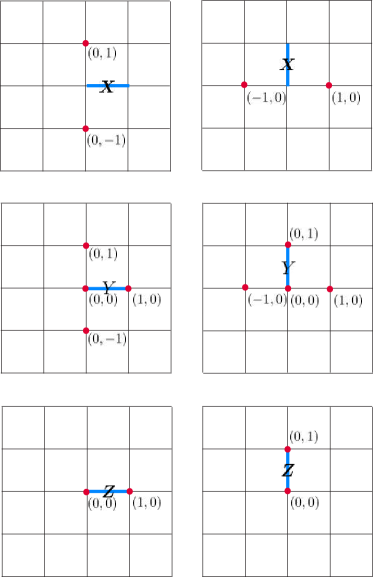
Figure 2: Syndromes of single-qubit errors for the bosonization with code distance $d=3$. The red vertices $v$ represent locations where the single-qubit error does not commute with the stabilizer $G_{v}$.

Given the stabilizer, we can provide the syndromes for all single-qubit Pauli errors, as shown in Fig. 2. We see that all single-qubit Pauli matrices have different syndromes, which means that we do not have any logical operators with weight 2. This implies a code distance of $d\geq 3$. Eq. (2.2) shows logical operators with weight 3, so we conclude that the code distance is $d=3$. Based on the syndrome measurements, we can always correct any single-qubit error according to Fig. 2.

The four types of nearest-neighbor hopping terms, $\gamma_{L}\gamma^{\prime}_{R}$, $\gamma_{L}\gamma_{R}$, $\gamma^{\prime}_{L}\gamma^{\prime}_{R}$, and $\gamma^{\prime}_{L}\gamma_{R}$ have weights $\text{wt}_{i}$ in the range $3\leq\text{wt}_{i}\leq 5$. Therefore, the modified bosonization has $(\text{wt}_{\mathrm{min}},\text{wt}_{\mathrm{max}})=(3,5)$ and a fermionic occupation term of weight 4. Compared to the original bosonization with $(\text{wt}_{\mathrm{min}},\text{wt}_{\mathrm{max}})=(2,6)$, the minimum weight is increased such that error correction can be performed, while the maximum weight of the hopping terms is decreased implying a reduction in the simulation cost.

Here we present the spinless Fermi-Hubbard Hamiltonian in 2d square lattice for $d=3$ encoding as a concrete example. The 2d spinless Fermi-Hubbard Hamiltonian is H=-t ∑_⟨i,j⟩(c_i^†c_j+h.c.)+U∑_⟨i,j⟩ c_i^†c_i c_j^†c_j, where $\langle i,j\rangle$ represents the nearest-neighbor pair of vertices in the square lattice. We can write individual terms in Majorana basis such as $c_{i}^{\dagger}c_{j}+\text{h.c.}=\frac{i}{2}(\gamma_{i}\gamma_{j}^{\prime}-\gamma_{i}^{\prime}\gamma_{j}),~{}c_{i}^{\dagger}c_{i}c_{j}^{\dagger}c_{j}=(\frac{1+i\gamma_{i}\gamma_{i}^{\prime}}{2})(\frac{1+i\gamma_{j}\gamma_{j}^{\prime}}{2})$. Next, we map the hopping terms and density-density interaction term to Pauli operators as follows γ_i γ_j’&   , ,
γ_i’ γ_j   , ,
-γ_iγ_i’ γ_j γ_j’     , , where two terms on the right-hand side correspond to vertical and horizontal $(i,j)$. The hopping terms have weights ranging from $3$ to $5$, and the interaction term has a weight $6$.

2.3 Bosonization with code distance $d=4$

In this subsection, we provide a construction of an exact bosonization with code distance $d=4$ as an intermediate step toward $d=5$. Since its code distance is $d=4$, which is even, this code (like the $d=3$ code) can only correct the $\lfloor\frac{d-1}{2}\rfloor=1$ Pauli error. However, for error defection, Pauli errors up to weight 3 can be observed from the stabilizer syndrome measurements.

The mapping can be described as

i× & ,
i× ,
-iγ_fγ_f’      . The stabilizer becomes

$$G^{d=4}_{v}=\hskip 8.5359pt\begin{gathered}\lx@xy@svg{\hbox{\raise 0.0pt\hbox{\kern 3.0pt\hbox{\ignorespaces\ignorespaces\ignorespaces\hbox{\vtop{\kern 0.0pt\offinterlineskip\halign{\entry@#!@&&\entry@@#!@\cr&&&\\&&&\\&&&\\&&&\crcr}}}\ignorespaces{\hbox{\kern-3.0pt\raise 0.0pt\hbox{\hbox{\kern 0.0pt\raise 0.0pt\hbox{\hbox{\kern 3.0pt\raise 0.0pt\hbox{$\textstyle{\ignorespaces\ignorespaces\ignorespaces\ignorespaces\ignorespaces}$}}}}}}}\ignorespaces\ignorespaces\ignorespaces\ignorespaces{}{\hbox{\lx@xy@droprule}}\ignorespaces{\hbox{\kern 14.75703pt\raise 0.0pt\hbox{\hbox{\kern 0.0pt\raise-3.41666pt\hbox{$\scriptstyle{\displaystyle Z}$}}}}}{\hbox{\lx@xy@droprule}}\ignorespaces{}{\hbox{\lx@xy@droprule}}{\hbox{\lx@xy@droprule}}{\hbox{\kern 34.05574pt\raise 0.0pt\hbox{\hbox{\kern 0.0pt\raise 0.0pt\hbox{\hbox{\kern 3.0pt\raise 0.0pt\hbox{$\textstyle{\ignorespaces\ignorespaces\ignorespaces\ignorespaces\ignorespaces}$}}}}}}}\ignorespaces\ignorespaces\ignorespaces\ignorespaces{}{\hbox{\lx@xy@droprule}}\ignorespaces{\hbox{\kern 32.52103pt\raise-17.22636pt\hbox{\hbox{\kern 0.0pt\raise-3.41666pt\hbox{$\scriptstyle{\displaystyle X}$}}}}}{\hbox{\lx@xy@droprule}}\ignorespaces{}{\hbox{\lx@xy@droprule}}{\hbox{\lx@xy@droprule}}{\hbox{\kern 71.11148pt\raise 0.0pt\hbox{\hbox{\kern 0.0pt\raise 0.0pt\hbox{\hbox{\kern 3.0pt\raise 0.0pt\hbox{$\textstyle{}$}}}}}}}{\hbox{\kern 105.56422pt\raise 0.0pt\hbox{\hbox{\kern 0.0pt\raise 0.0pt\hbox{\hbox{\kern 3.0pt\raise 0.0pt\hbox{$\textstyle{}$}}}}}}}{\hbox{\kern-3.0pt\raise-34.45274pt\hbox{\hbox{\kern 0.0pt\raise 0.0pt\hbox{\hbox{\kern 3.0pt\raise 0.0pt\hbox{$\textstyle{}$}}}}}}}{\hbox{\kern 34.05574pt\raise-34.45274pt\hbox{\hbox{\kern 0.0pt\raise 0.0pt\hbox{\hbox{\kern 3.0pt\raise 0.0pt\hbox{$\textstyle{{}\ignorespaces\ignorespaces\ignorespaces\ignorespaces\ignorespaces\ignorespaces\ignorespaces\ignorespaces\ignorespaces\ignorespaces}$}}}}}}}\ignorespaces\ignorespaces\ignorespaces\ignorespaces{}{\hbox{\lx@xy@droprule}}\ignorespaces{\hbox{\kern 33.28491pt\raise-52.7555pt\hbox{\hbox{\kern 0.0pt\raise-3.41666pt\hbox{$\scriptstyle{\displaystyle Z}$}}}}}{\hbox{\lx@xy@droprule}}\ignorespaces{}{\hbox{\lx@xy@droprule}}{\hbox{\lx@xy@droprule}}\ignorespaces\ignorespaces\ignorespaces\ignorespaces{}{\hbox{\lx@xy@droprule}}\ignorespaces{\hbox{\kern 51.81277pt\raise-34.45274pt\hbox{\hbox{\kern 0.0pt\raise-3.41666pt\hbox{$\scriptstyle{\displaystyle Z}$}}}}}{\hbox{\lx@xy@droprule}}\ignorespaces{}{\hbox{\lx@xy@droprule}}{\hbox{\lx@xy@droprule}}{\hbox{\kern 71.11148pt\raise-34.45274pt\hbox{\hbox{\kern 0.0pt\raise 0.0pt\hbox{\hbox{\kern 3.0pt\raise 0.0pt\hbox{$\textstyle{}$}}}}}}}{\hbox{\kern 105.56422pt\raise-34.45274pt\hbox{\hbox{\kern 0.0pt\raise 0.0pt\hbox{\hbox{\kern 3.0pt\raise 0.0pt\hbox{$\textstyle{}$}}}}}}}{\hbox{\kern-3.0pt\raise-71.05826pt\hbox{\hbox{\kern 0.0pt\raise 0.0pt\hbox{\hbox{\kern 3.0pt\raise 0.0pt\hbox{$\textstyle{{}\ignorespaces\ignorespaces\ignorespaces\ignorespaces\ignorespaces}$}}}}}}}\ignorespaces\ignorespaces\ignorespaces\ignorespaces{}{\hbox{\lx@xy@droprule}}\ignorespaces{\hbox{\kern 10.22232pt\raise-71.05826pt\hbox{\hbox{\kern 0.0pt\raise-3.41666pt\hbox{$\scriptstyle{\displaystyle XZ}$}}}}}{\hbox{\lx@xy@droprule}}\ignorespaces{}{\hbox{\lx@xy@droprule}}{\hbox{\lx@xy@droprule}}{\hbox{\kern 31.45274pt\raise-71.05826pt\hbox{\hbox{\kern 0.0pt\raise 0.0pt\hbox{\hbox{\kern 3.0pt\raise 0.0pt\hbox{$\textstyle{{v}\ignorespaces\ignorespaces\ignorespaces\ignorespaces\ignorespaces\ignorespaces\ignorespaces\ignorespaces\ignorespaces\ignorespaces}$}}}}}}}\ignorespaces\ignorespaces\ignorespaces\ignorespaces{}{\hbox{\lx@xy@droprule}}\ignorespaces{\hbox{\kern 51.81277pt\raise-71.05826pt\hbox{\hbox{\kern 0.0pt\raise-3.41666pt\hbox{$\scriptstyle{\displaystyle Z}$}}}}}{\hbox{\lx@xy@droprule}}\ignorespaces{}{\hbox{\lx@xy@droprule}}{\hbox{\lx@xy@droprule}}\ignorespaces\ignorespaces\ignorespaces\ignorespaces{}{\hbox{\lx@xy@droprule}}\ignorespaces{\hbox{\kern 28.7502pt\raise-89.36101pt\hbox{\hbox{\kern 0.0pt\raise-3.41666pt\hbox{$\scriptstyle{\displaystyle XZ}$}}}}}{\hbox{\lx@xy@droprule}}\ignorespaces{}{\hbox{\lx@xy@droprule}}{\hbox{\lx@xy@droprule}}{\hbox{\kern 71.11148pt\raise-71.05826pt\hbox{\hbox{\kern 0.0pt\raise 0.0pt\hbox{\hbox{\kern 3.0pt\raise 0.0pt\hbox{$\textstyle{\ignorespaces\ignorespaces\ignorespaces\ignorespaces\ignorespaces\ignorespaces\ignorespaces\ignorespaces\ignorespaces\ignorespaces}$}}}}}}}\ignorespaces\ignorespaces\ignorespaces\ignorespaces{}{\hbox{\lx@xy@droprule}}\ignorespaces{\hbox{\kern 86.80313pt\raise-71.05826pt\hbox{\hbox{\kern 0.0pt\raise-3.41666pt\hbox{$\scriptstyle{\displaystyle X}$}}}}}{\hbox{\lx@xy@droprule}}\ignorespaces{}{\hbox{\lx@xy@droprule}}{\hbox{\lx@xy@droprule}}\ignorespaces\ignorespaces\ignorespaces\ignorespaces{}{\hbox{\lx@xy@droprule}}\ignorespaces{\hbox{\kern 70.34065pt\raise-52.75551pt\hbox{\hbox{\kern 0.0pt\raise-3.41666pt\hbox{$\scriptstyle{\displaystyle Z}$}}}}}{\hbox{\lx@xy@droprule}}\ignorespaces{}{\hbox{\lx@xy@droprule}}{\hbox{\lx@xy@droprule}}{\hbox{\kern 105.56422pt\raise-71.05826pt\hbox{\hbox{\kern 0.0pt\raise 0.0pt\hbox{\hbox{\kern 3.0pt\raise 0.0pt\hbox{$\textstyle{\ignorespaces\ignorespaces\ignorespaces\ignorespaces\ignorespaces}$}}}}}}}\ignorespaces\ignorespaces\ignorespaces\ignorespaces{}{\hbox{\lx@xy@droprule}}\ignorespaces{\hbox{\kern 104.7934pt\raise-89.36101pt\hbox{\hbox{\kern 0.0pt\raise-3.41666pt\hbox{$\scriptstyle{\displaystyle Z}$}}}}}{\hbox{\lx@xy@droprule}}\ignorespaces{}{\hbox{\lx@xy@droprule}}{\hbox{\lx@xy@droprule}}{\hbox{\kern-3.0pt\raise-107.66377pt\hbox{\hbox{\kern 0.0pt\raise 0.0pt\hbox{\hbox{\kern 3.0pt\raise 0.0pt\hbox{$\textstyle{}$}}}}}}}{\hbox{\kern 34.05574pt\raise-107.66377pt\hbox{\hbox{\kern 0.0pt\raise 0.0pt\hbox{\hbox{\kern 3.0pt\raise 0.0pt\hbox{$\textstyle{}$}}}}}}}{\hbox{\kern 71.11148pt\raise-107.66377pt\hbox{\hbox{\kern 0.0pt\raise 0.0pt\hbox{\hbox{\kern 3.0pt\raise 0.0pt\hbox{$\textstyle{}$}}}}}}}{\hbox{\kern 105.56422pt\raise-107.66377pt\hbox{\hbox{\kern 0.0pt\raise 0.0pt\hbox{\hbox{\kern 3.0pt\raise 0.0pt\hbox{$\textstyle{}$}}}}}}}\ignorespaces}}}}\ignorespaces\end{gathered}\quad=1. \scriptstyle{\displaystyle Z} \scriptstyle{\displaystyle X} \scriptstyle{\displaystyle Z} \scriptstyle{\displaystyle Z} \scriptstyle{\displaystyle XZ} \textstyle{{v}\ignorespaces\ignorespaces\ignorespaces\ignorespaces\ignorespaces\ignorespaces\ignorespaces\ignorespaces\ignorespaces\ignorespaces} \scriptstyle{\displaystyle Z} \scriptstyle{\displaystyle XZ} \scriptstyle{\displaystyle X} \scriptstyle{\displaystyle Z} \scriptstyle{\displaystyle Z}$$ (10)

We can check that the logical operators in Eq. (2.3) commute with the stabilizer in Eq. (10). The proof of the equivalence between the even fermionic algebra and this stabilizer code will be shown in Section. 3.

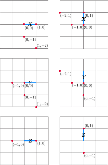
Figure 3: Syndromes of single-qubit errors for the bosonization with code distance $d=4$. The red vertices $v$ represent locations where the single-qubit error does not commute with the stabilizer $G^{d=4}_{v}$.

The syndromes for all single-qubit Pauli errors are provided in Fig. 3. From the generators of the logical operators in Eq. (2.3), we may be tempted to conclude that the code distance is $d=5$ because the minimum weight is 5. However, based on the syndromes in Fig. 3, we find that the following operator is logical:  . Since it does not commute with the terms in Eq. (2.3), this operator does not belong to the stabilizer group. Therefore, the code distance for this stabilizer code is $d\leq 4$. In Appendix LABEL:sec:_syndrome_matching_method, we introduce the “syndrome matching” method to provide a lower bound for the code distance for a given stabilizer code. With this method, we check that the stabilizer code defined by Eq. (10) has a code distance of $d=4$.

The minimum and maximum weights of the nearest-neighbor terms are $(\text{wt}_{\mathrm{min}},\text{wt}_{\mathrm{max}})=(5,6)$ and the fermionic occupation term has weight 6, which means that all the operations are quite well-balanced. This code has an error-correcting property for any single-qubit error.

2.4 Bosonization with code distance $d=5$

The bosonization map with code distance $d=5$ is provided in this subsection. The generators of the even fermionic algebra are mapped to Pauli matrices as shown below:

$$i\begin{gathered}\lx@xy@svg{\hbox{\raise 0.0pt\hbox{\kern 3.0pt\hbox{\ignorespaces\ignorespaces\ignorespaces\hbox{\vtop{\kern 0.0pt\offinterlineskip\halign{\entry@#!@&&\entry@@#!@\cr&\\&\\&\crcr}}}\ignorespaces{\hbox{\kern-3.0pt\raise 0.0pt\hbox{\hbox{\kern 0.0pt\raise 0.0pt\hbox{\hbox{\kern 3.0pt\raise 0.0pt\hbox{$\textstyle{}$}}}}}}}{\hbox{\kern 37.14322pt\raise 0.0pt\hbox{\hbox{\kern 0.0pt\raise 0.0pt\hbox{\hbox{\kern 3.0pt\raise 0.0pt\hbox{$\textstyle{}$}}}}}}}{\hbox{\kern-3.0pt\raise-40.14322pt\hbox{\hbox{\kern 0.0pt\raise 0.0pt\hbox{\hbox{\kern 3.0pt\raise 0.0pt\hbox{$\textstyle{{}\ignorespaces\ignorespaces\ignorespaces\ignorespaces\ignorespaces\ignorespaces\ignorespaces\ignorespaces\ignorespaces}$}}}}}}}\ignorespaces\ignorespaces\ignorespaces\ignorespaces{}\ignorespaces{\hbox{\kern 11.92107pt\raise-20.0718pt\hbox{\hbox{\kern 0.0pt\raise-0.37001pt\hbox{$\scriptstyle{{{\gamma_{L(e)}}}}$}}}}}\ignorespaces{}\ignorespaces\ignorespaces\ignorespaces\ignorespaces{}{\hbox{\lx@xy@droprule}}\ignorespaces\ignorespaces\ignorespaces{\hbox{\kern 15.11598pt\raise-35.33488pt\hbox{{}\hbox{\kern 0.0pt\raise 0.0pt\hbox{\hbox{\kern 3.0pt\hbox{\hbox{\kern 0.0pt\raise-1.80833pt\hbox{$\scriptstyle{e}$}}}\kern 3.0pt}}}}}}\ignorespaces{}{\hbox{\lx@xy@droprule}}{\hbox{\lx@xy@droprule}}{\hbox{\kern 37.14322pt\raise-40.14322pt\hbox{\hbox{\kern 0.0pt\raise 0.0pt\hbox{\hbox{\kern 3.0pt\raise 0.0pt\hbox{$\textstyle{}$}}}}}}}{\hbox{\kern-3.0pt\raise-80.28644pt\hbox{\hbox{\kern 0.0pt\raise 0.0pt\hbox{\hbox{\kern 3.0pt\raise 0.0pt\hbox{$\textstyle{\ignorespaces\ignorespaces\ignorespaces\ignorespaces\ignorespaces}$}}}}}}}\ignorespaces\ignorespaces\ignorespaces\ignorespaces{}\ignorespaces{\hbox{\kern 16.67007pt\raise-60.21501pt\hbox{\hbox{\kern 0.0pt\raise-1.17001pt\hbox{$\scriptstyle{{{\gamma^{\prime}_{R(e)}}}}$}}}}}\ignorespaces{}{\hbox{\kern 37.14322pt\raise-80.28644pt\hbox{\hbox{\kern 0.0pt\raise 0.0pt\hbox{\hbox{\kern 3.0pt\raise 0.0pt\hbox{$\textstyle{}$}}}}}}}\ignorespaces}}}}\ignorespaces\end{gathered} \scriptstyle{{{\gamma_{L(e)}}}} \scriptstyle{e} \scriptstyle{{{\gamma^{\prime}_{R(e)}}}} \scriptstyle{{{\gamma_{L(e)}}}} \scriptstyle{e} \scriptstyle{{{\gamma^{\prime}_{R(e)}}}} \begin{gathered}\lx@xy@svg{\hbox{\raise 0.0pt\hbox{\kern 3.0pt\hbox{\ignorespaces\ignorespaces\ignorespaces\hbox{\vtop{\kern 0.0pt\offinterlineskip\halign{\entry@#!@&&\entry@@#!@\cr&\crcr}}}\ignorespaces{\hbox{\kern-3.0pt\raise 0.0pt\hbox{\hbox{\kern 0.0pt\raise 0.0pt\hbox{\hbox{\kern 3.0pt\raise 0.0pt\hbox{$\textstyle{{}\ignorespaces\ignorespaces\ignorespaces\ignorespaces}$}}}}}}}\ignorespaces\ignorespaces\ignorespaces\ignorespaces{\hbox{\kern 3.0pt\raise 0.0pt\hbox{\hbox{\kern 0.0pt\raise 0.0pt\hbox{\lx@xy@tip{1}\lx@xy@tip{-1}}}}}}{\hbox{\lx@xy@droprule}}\ignorespaces{\hbox{\kern 27.0pt\raise 0.0pt\hbox{\hbox{\kern 0.0pt\raise 0.0pt\hbox{\lx@xy@tip{1}\lx@xy@tip{-1}}}}}}{\hbox{\lx@xy@droprule}}{\hbox{\lx@xy@droprule}}{\hbox{\kern 27.0pt\raise 0.0pt\hbox{\hbox{\kern 0.0pt\raise 0.0pt\hbox{\hbox{\kern 3.0pt\raise 0.0pt\hbox{$\textstyle{}$}}}}}}}\ignorespaces}}}}\ignorespaces\end{gathered}\begin{gathered}\lx@xy@svg{\hbox{\raise 0.0pt\hbox{\kern 8.30554pt\hbox{\ignorespaces\ignorespaces\ignorespaces\hbox{\vtop{\kern 0.0pt\offinterlineskip\halign{\entry@#!@&&\entry@@#!@\cr&&\\&&\\&&\crcr}}}\ignorespaces{\hbox{\kern-3.0pt\raise 0.0pt\hbox{\hbox{\kern 0.0pt\raise 0.0pt\hbox{\hbox{\kern 3.0pt\raise 0.0pt\hbox{$\textstyle{{}\ignorespaces\ignorespaces\ignorespaces\ignorespaces\ignorespaces}$}}}}}}}\ignorespaces\ignorespaces\ignorespaces\ignorespaces{}{\hbox{\lx@xy@droprule}}\ignorespaces{\hbox{\kern-4.53471pt\raise-17.22636pt\hbox{\hbox{\kern 0.0pt\raise-3.41666pt\hbox{$\scriptstyle{\displaystyle X}$}}}}}{\hbox{\lx@xy@droprule}}\ignorespaces{}{\hbox{\lx@xy@droprule}}{\hbox{\lx@xy@droprule}}{\hbox{\kern 31.45274pt\raise 0.0pt\hbox{\hbox{\kern 0.0pt\raise 0.0pt\hbox{\hbox{\kern 3.0pt\raise 0.0pt\hbox{$\textstyle{{}\ignorespaces\ignorespaces\ignorespaces\ignorespaces\ignorespaces}$}}}}}}}\ignorespaces\ignorespaces\ignorespaces\ignorespaces{}{\hbox{\lx@xy@droprule}}\ignorespaces{\hbox{\kern 30.68192pt\raise-17.22636pt\hbox{\hbox{\kern 0.0pt\raise-3.41666pt\hbox{$\scriptstyle{\displaystyle Z}$}}}}}{\hbox{\lx@xy@droprule}}\ignorespaces{}{\hbox{\lx@xy@droprule}}{\hbox{\lx@xy@droprule}}{\hbox{\kern 65.90549pt\raise 0.0pt\hbox{\hbox{\kern 0.0pt\raise 0.0pt\hbox{\hbox{\kern 3.0pt\raise 0.0pt\hbox{$\textstyle{}$}}}}}}}{\hbox{\kern-3.0pt\raise-34.45274pt\hbox{\hbox{\kern 0.0pt\raise 0.0pt\hbox{\hbox{\kern 3.0pt\raise 0.0pt\hbox{$\textstyle{{}\ignorespaces\ignorespaces\ignorespaces\ignorespaces\ignorespaces}$}}}}}}}\ignorespaces\ignorespaces\ignorespaces\ignorespaces{}{\hbox{\lx@xy@droprule}}\ignorespaces{\hbox{\kern 11.3879pt\raise-34.45274pt\hbox{\hbox{\kern 0.0pt\raise-2.81389pt\hbox{$\scriptstyle{\displaystyle X_{e}}$}}}}}{\hbox{\lx@xy@droprule}}\ignorespaces{}{\hbox{\lx@xy@droprule}}{\hbox{\lx@xy@droprule}}{\hbox{\kern 31.45274pt\raise-34.45274pt\hbox{\hbox{\kern 0.0pt\raise 0.0pt\hbox{\hbox{\kern 3.0pt\raise 0.0pt\hbox{$\textstyle{\ignorespaces\ignorespaces\ignorespaces\ignorespaces\ignorespaces}$}}}}}}}\ignorespaces\ignorespaces\ignorespaces\ignorespaces{}{\hbox{\lx@xy@droprule}}\ignorespaces{\hbox{\kern 47.90828pt\raise-34.45274pt\hbox{\hbox{\kern 0.0pt\raise-3.41666pt\hbox{$\scriptstyle{\displaystyle Z}$}}}}}{\hbox{\lx@xy@droprule}}\ignorespaces{}{\hbox{\lx@xy@droprule}}{\hbox{\lx@xy@droprule}}{\hbox{\kern 65.90549pt\raise-34.45274pt\hbox{\hbox{\kern 0.0pt\raise 0.0pt\hbox{\hbox{\kern 3.0pt\raise 0.0pt\hbox{$\textstyle{}$}}}}}}}{\hbox{\kern-3.0pt\raise-68.90549pt\hbox{\hbox{\kern 0.0pt\raise 0.0pt\hbox{\hbox{\kern 3.0pt\raise 0.0pt\hbox{$\textstyle{{}\ignorespaces\ignorespaces\ignorespaces\ignorespaces\ignorespaces\ignorespaces\ignorespaces\ignorespaces\ignorespaces\ignorespaces}$}}}}}}}\ignorespaces\ignorespaces\ignorespaces\ignorespaces{}{\hbox{\lx@xy@droprule}}\ignorespaces{\hbox{\kern-8.30554pt\raise-51.67912pt\hbox{\hbox{\kern 0.0pt\raise-3.41666pt\hbox{$\scriptstyle{\displaystyle XZ}$}}}}}{\hbox{\lx@xy@droprule}}\ignorespaces{}{\hbox{\lx@xy@droprule}}{\hbox{\lx@xy@droprule}}\ignorespaces\ignorespaces\ignorespaces\ignorespaces{}{\hbox{\lx@xy@droprule}}\ignorespaces{\hbox{\kern 8.92082pt\raise-68.90549pt\hbox{\hbox{\kern 0.0pt\raise-3.41666pt\hbox{$\scriptstyle{\displaystyle XZ}$}}}}}{\hbox{\lx@xy@droprule}}\ignorespaces{}{\hbox{\lx@xy@droprule}}{\hbox{\lx@xy@droprule}}{\hbox{\kern 31.45274pt\raise-68.90549pt\hbox{\hbox{\kern 0.0pt\raise 0.0pt\hbox{\hbox{\kern 3.0pt\raise 0.0pt\hbox{$\textstyle{\ignorespaces\ignorespaces\ignorespaces\ignorespaces\ignorespaces\ignorespaces\ignorespaces\ignorespaces\ignorespaces\ignorespaces\ignorespaces\ignorespaces\ignorespaces\ignorespaces\ignorespaces}$}}}}}}}\ignorespaces\ignorespaces\ignorespaces\ignorespaces{}{\hbox{\lx@xy@droprule}}\ignorespaces{\hbox{\kern 30.68192pt\raise-51.67912pt\hbox{\hbox{\kern 0.0pt\raise-3.41666pt\hbox{$\scriptstyle{\displaystyle Z}$}}}}}{\hbox{\lx@xy@droprule}}\ignorespaces{}{\hbox{\lx@xy@droprule}}{\hbox{\lx@xy@droprule}}\ignorespaces\ignorespaces\ignorespaces\ignorespaces{}{\hbox{\lx@xy@droprule}}\ignorespaces{\hbox{\kern 30.68192pt\raise-51.67912pt\hbox{\hbox{\kern 0.0pt\raise-3.41666pt\hbox{$\scriptstyle{\displaystyle Z}$}}}}}{\hbox{\lx@xy@droprule}}\ignorespaces{}{\hbox{\lx@xy@droprule}}{\hbox{\lx@xy@droprule}}\ignorespaces\ignorespaces\ignorespaces\ignorespaces{}{\hbox{\lx@xy@droprule}}\ignorespaces{\hbox{\kern 47.90828pt\raise-68.90549pt\hbox{\hbox{\kern 0.0pt\raise-3.41666pt\hbox{$\scriptstyle{\displaystyle Z}$}}}}}{\hbox{\lx@xy@droprule}}\ignorespaces{}{\hbox{\lx@xy@droprule}}{\hbox{\lx@xy@droprule}}{\hbox{\kern 65.90549pt\raise-68.90549pt\hbox{\hbox{\kern 0.0pt\raise 0.0pt\hbox{\hbox{\kern 3.0pt\raise 0.0pt\hbox{$\textstyle{}$}}}}}}}\ignorespaces}}}}\ignorespaces\end{gathered}, \scriptstyle{\displaystyle X} \scriptstyle{\displaystyle Z} \scriptstyle{\displaystyle X_{e}} \scriptstyle{\displaystyle Z} \scriptstyle{\displaystyle XZ} \scriptstyle{\displaystyle XZ} \scriptstyle{\displaystyle Z} \scriptstyle{\displaystyle Z} \scriptstyle{\displaystyle Z} \scriptstyle{\displaystyle X} \scriptstyle{\displaystyle Z} \scriptstyle{\displaystyle X_{e}} \scriptstyle{\displaystyle Z} \scriptstyle{\displaystyle XZ} \scriptstyle{\displaystyle XZ} \scriptstyle{\displaystyle Z} \scriptstyle{\displaystyle Z} \scriptstyle{\displaystyle Z}$$ (28)

$$\begin{gathered}\lx@xy@svg{\hbox{\raise 0.0pt\hbox{\kern 3.0pt\hbox{\ignorespaces\ignorespaces\ignorespaces\hbox{\vtop{\kern 0.0pt\offinterlineskip\halign{\entry@#!@&&\entry@@#!@\cr&&\\&&\crcr}}}\ignorespaces{\hbox{\kern-3.0pt\raise 0.0pt\hbox{\hbox{\kern 0.0pt\raise 0.0pt\hbox{\hbox{\kern 3.0pt\raise 0.0pt\hbox{$\textstyle{}$}}}}}}}{\hbox{\kern 37.14322pt\raise 0.0pt\hbox{\hbox{\kern 0.0pt\raise 0.0pt\hbox{\hbox{\kern 3.0pt\raise 0.0pt\hbox{$\textstyle{{}\ignorespaces\ignorespaces\ignorespaces\ignorespaces}$}}}}}}}\ignorespaces\ignorespaces\ignorespaces\ignorespaces{}{\hbox{\lx@xy@droprule}}\ignorespaces\ignorespaces\ignorespaces{\hbox{\kern 40.14322pt\raise-20.07161pt\hbox{{}\hbox{\kern 0.0pt\raise 0.0pt\hbox{\hbox{\kern 3.0pt\hbox{\hbox{\kern 0.0pt\raise-1.80833pt\hbox{$\scriptstyle{e}$}}}\kern 3.0pt}}}}}}\ignorespaces{}{\hbox{\lx@xy@droprule}}{\hbox{\lx@xy@droprule}}{\hbox{\kern 77.28644pt\raise 0.0pt\hbox{\hbox{\kern 0.0pt\raise 0.0pt\hbox{\hbox{\kern 3.0pt\raise 0.0pt\hbox{$\textstyle{}$}}}}}}}{\hbox{\kern-3.0pt\raise-40.14322pt\hbox{\hbox{\kern 0.0pt\raise 0.0pt\hbox{\hbox{\kern 3.0pt\raise 0.0pt\hbox{$\textstyle{\ignorespaces\ignorespaces\ignorespaces\ignorespaces\ignorespaces}$}}}}}}}\ignorespaces\ignorespaces\ignorespaces\ignorespaces{}\ignorespaces{\hbox{\kern 10.18472pt\raise-20.0718pt\hbox{\hbox{\kern 0.0pt\raise-1.52402pt\hbox{$\scriptstyle{{{i\gamma_{L(e)}}}}$}}}}}\ignorespaces{}{\hbox{\kern 37.14322pt\raise-40.14322pt\hbox{\hbox{\kern 0.0pt\raise 0.0pt\hbox{\hbox{\kern 3.0pt\raise 0.0pt\hbox{$\textstyle{\ignorespaces\ignorespaces\ignorespaces\ignorespaces\ignorespaces}$}}}}}}}\ignorespaces\ignorespaces\ignorespaces\ignorespaces{}\ignorespaces{\hbox{\kern 53.31328pt\raise-20.0718pt\hbox{\hbox{\kern 0.0pt\raise-1.17001pt\hbox{$\scriptstyle{\quad{{\gamma^{\prime}_{R(e)}}}}$}}}}}\ignorespaces{}{\hbox{\kern 77.28644pt\raise-40.14322pt\hbox{\hbox{\kern 0.0pt\raise 0.0pt\hbox{\hbox{\kern 3.0pt\raise 0.0pt\hbox{$\textstyle{}$}}}}}}}\ignorespaces}}}}\ignorespaces\end{gathered} \scriptstyle{e} \scriptstyle{{{i\gamma_{L(e)}}}} \scriptstyle{\quad{{\gamma^{\prime}_{R(e)}}}} \scriptstyle{e} \scriptstyle{{{i\gamma_{L(e)}}}} \scriptstyle{\quad{{\gamma^{\prime}_{R(e)}}}} \begin{gathered}\lx@xy@svg{\hbox{\raise 0.0pt\hbox{\kern 3.0pt\hbox{\ignorespaces\ignorespaces\ignorespaces\hbox{\vtop{\kern 0.0pt\offinterlineskip\halign{\entry@#!@&&\entry@@#!@\cr&\crcr}}}\ignorespaces{\hbox{\kern-3.0pt\raise 0.0pt\hbox{\hbox{\kern 0.0pt\raise 0.0pt\hbox{\hbox{\kern 3.0pt\raise 0.0pt\hbox{$\textstyle{{}\ignorespaces\ignorespaces\ignorespaces\ignorespaces}$}}}}}}}\ignorespaces\ignorespaces\ignorespaces\ignorespaces{\hbox{\kern 3.0pt\raise 0.0pt\hbox{\hbox{\kern 0.0pt\raise 0.0pt\hbox{\lx@xy@tip{1}\lx@xy@tip{-1}}}}}}{\hbox{\lx@xy@droprule}}\ignorespaces{\hbox{\kern 27.0pt\raise 0.0pt\hbox{\hbox{\kern 0.0pt\raise 0.0pt\hbox{\lx@xy@tip{1}\lx@xy@tip{-1}}}}}}{\hbox{\lx@xy@droprule}}{\hbox{\lx@xy@droprule}}{\hbox{\kern 27.0pt\raise 0.0pt\hbox{\hbox{\kern 0.0pt\raise 0.0pt\hbox{\hbox{\kern 3.0pt\raise 0.0pt\hbox{$\textstyle{}$}}}}}}}\ignorespaces}}}}\ignorespaces\end{gathered}\begin{gathered}\lx@xy@svg{\hbox{\raise 0.0pt\hbox{\kern 3.0pt\hbox{\ignorespaces\ignorespaces\ignorespaces\hbox{\vtop{\kern 0.0pt\offinterlineskip\halign{\entry@#!@&&\entry@@#!@\cr&&&&\\&&&&\crcr}}}\ignorespaces{\hbox{\kern-3.0pt\raise 0.0pt\hbox{\hbox{\kern 0.0pt\raise 0.0pt\hbox{\hbox{\kern 3.0pt\raise 0.0pt\hbox{$\textstyle{}$}}}}}}}{\hbox{\kern 31.45274pt\raise 0.0pt\hbox{\hbox{\kern 0.0pt\raise 0.0pt\hbox{\hbox{\kern 3.0pt\raise 0.0pt\hbox{$\textstyle{}$}}}}}}}{\hbox{\kern 65.90549pt\raise 0.0pt\hbox{\hbox{\kern 0.0pt\raise 0.0pt\hbox{\hbox{\kern 3.0pt\raise 0.0pt\hbox{$\textstyle{\ignorespaces\ignorespaces\ignorespaces\ignorespaces}$}}}}}}}\ignorespaces\ignorespaces\ignorespaces\ignorespaces{}{\hbox{\lx@xy@droprule}}\ignorespaces\ignorespaces\ignorespaces{\hbox{\kern 68.90549pt\raise-17.22636pt\hbox{{}\hbox{\kern 0.0pt\raise 0.0pt\hbox{\hbox{\kern 3.0pt\hbox{\hbox{\kern 0.0pt\raise-1.80833pt\hbox{$\scriptstyle{e}$}}}\kern 3.0pt}}}}}}\ignorespaces{}{\hbox{\lx@xy@droprule}}{\hbox{\lx@xy@droprule}}{\hbox{\kern 100.35823pt\raise 0.0pt\hbox{\hbox{\kern 0.0pt\raise 0.0pt\hbox{\hbox{\kern 3.0pt\raise 0.0pt\hbox{$\textstyle{}$}}}}}}}{\hbox{\kern 134.81097pt\raise 0.0pt\hbox{\hbox{\kern 0.0pt\raise 0.0pt\hbox{\hbox{\kern 3.0pt\raise 0.0pt\hbox{$\textstyle{}$}}}}}}}{\hbox{\kern-3.0pt\raise-34.45274pt\hbox{\hbox{\kern 0.0pt\raise 0.0pt\hbox{\hbox{\kern 3.0pt\raise 0.0pt\hbox{$\textstyle{{}\ignorespaces\ignorespaces\ignorespaces\ignorespaces\ignorespaces}$}}}}}}}\ignorespaces\ignorespaces\ignorespaces\ignorespaces{}{\hbox{\lx@xy@droprule}}\ignorespaces{\hbox{\kern 13.45554pt\raise-34.45274pt\hbox{\hbox{\kern 0.0pt\raise-3.41666pt\hbox{$\scriptstyle{\displaystyle Z}$}}}}}{\hbox{\lx@xy@droprule}}\ignorespaces{}{\hbox{\lx@xy@droprule}}{\hbox{\lx@xy@droprule}}{\hbox{\kern 31.45274pt\raise-34.45274pt\hbox{\hbox{\kern 0.0pt\raise 0.0pt\hbox{\hbox{\kern 3.0pt\raise 0.0pt\hbox{$\textstyle{\ignorespaces\ignorespaces\ignorespaces\ignorespaces\ignorespaces}$}}}}}}}\ignorespaces\ignorespaces\ignorespaces\ignorespaces{}{\hbox{\lx@xy@droprule}}\ignorespaces{\hbox{\kern 47.1444pt\raise-34.45274pt\hbox{\hbox{\kern 0.0pt\raise-3.41666pt\hbox{$\scriptstyle{\displaystyle X}$}}}}}{\hbox{\lx@xy@droprule}}\ignorespaces{}{\hbox{\lx@xy@droprule}}{\hbox{\lx@xy@droprule}}{\hbox{\kern 65.90549pt\raise-34.45274pt\hbox{\hbox{\kern 0.0pt\raise 0.0pt\hbox{\hbox{\kern 3.0pt\raise 0.0pt\hbox{$\textstyle{{}\ignorespaces\ignorespaces\ignorespaces\ignorespaces\ignorespaces}$}}}}}}}\ignorespaces\ignorespaces\ignorespaces\ignorespaces{}{\hbox{\lx@xy@droprule}}\ignorespaces{\hbox{\kern 81.59714pt\raise-34.45274pt\hbox{\hbox{\kern 0.0pt\raise-3.41666pt\hbox{$\scriptstyle{\displaystyle X}$}}}}}{\hbox{\lx@xy@droprule}}\ignorespaces{}{\hbox{\lx@xy@droprule}}{\hbox{\lx@xy@droprule}}{\hbox{\kern 100.35823pt\raise-34.45274pt\hbox{\hbox{\kern 0.0pt\raise 0.0pt\hbox{\hbox{\kern 3.0pt\raise 0.0pt\hbox{$\textstyle{\ignorespaces\ignorespaces\ignorespaces\ignorespaces\ignorespaces\ignorespaces\ignorespaces\ignorespaces\ignorespaces\ignorespaces}$}}}}}}}\ignorespaces\ignorespaces\ignorespaces\ignorespaces{}{\hbox{\lx@xy@droprule}}\ignorespaces{\hbox{\kern 116.81377pt\raise-34.45274pt\hbox{\hbox{\kern 0.0pt\raise-3.41666pt\hbox{$\scriptstyle{\displaystyle Z}$}}}}}{\hbox{\lx@xy@droprule}}\ignorespaces{}{\hbox{\lx@xy@droprule}}{\hbox{\lx@xy@droprule}}\ignorespaces\ignorespaces\ignorespaces\ignorespaces{}{\hbox{\lx@xy@droprule}}\ignorespaces{\hbox{\kern 99.5874pt\raise-17.22638pt\hbox{\hbox{\kern 0.0pt\raise-3.41666pt\hbox{$\scriptstyle{\displaystyle Z}$}}}}}{\hbox{\lx@xy@droprule}}\ignorespaces{}{\hbox{\lx@xy@droprule}}{\hbox{\lx@xy@droprule}}{\hbox{\kern 134.81097pt\raise-34.45274pt\hbox{\hbox{\kern 0.0pt\raise 0.0pt\hbox{\hbox{\kern 3.0pt\raise 0.0pt\hbox{$\textstyle{}$}}}}}}}\ignorespaces}}}}\ignorespaces\end{gathered}, \scriptstyle{e} \scriptstyle{\displaystyle Z} \scriptstyle{\displaystyle X} \scriptstyle{\displaystyle X} \scriptstyle{\displaystyle Z} \scriptstyle{\displaystyle Z} \scriptstyle{e} \scriptstyle{\displaystyle Z} \scriptstyle{\displaystyle X} \scriptstyle{\displaystyle X} \scriptstyle{\displaystyle Z} \scriptstyle{\displaystyle Z}$$ (42)

$$-i\gamma_{f}\gamma_{f}^{\prime} \begin{gathered}\lx@xy@svg{\hbox{\raise 0.0pt\hbox{\kern 3.0pt\hbox{\ignorespaces\ignorespaces\ignorespaces\hbox{\vtop{\kern 0.0pt\offinterlineskip\halign{\entry@#!@&&\entry@@#!@\cr&\crcr}}}\ignorespaces{\hbox{\kern-3.0pt\raise 0.0pt\hbox{\hbox{\kern 0.0pt\raise 0.0pt\hbox{\hbox{\kern 3.0pt\raise 0.0pt\hbox{$\textstyle{{}\ignorespaces\ignorespaces\ignorespaces\ignorespaces}$}}}}}}}\ignorespaces\ignorespaces\ignorespaces\ignorespaces{\hbox{\kern 3.0pt\raise 0.0pt\hbox{\hbox{\kern 0.0pt\raise 0.0pt\hbox{\lx@xy@tip{1}\lx@xy@tip{-1}}}}}}{\hbox{\lx@xy@droprule}}\ignorespaces{\hbox{\kern 27.0pt\raise 0.0pt\hbox{\hbox{\kern 0.0pt\raise 0.0pt\hbox{\lx@xy@tip{1}\lx@xy@tip{-1}}}}}}{\hbox{\lx@xy@droprule}}{\hbox{\lx@xy@droprule}}{\hbox{\kern 27.0pt\raise 0.0pt\hbox{\hbox{\kern 0.0pt\raise 0.0pt\hbox{\hbox{\kern 3.0pt\raise 0.0pt\hbox{$\textstyle{}$}}}}}}}\ignorespaces}}}}\ignorespaces\end{gathered}\hskip 8.5359pt\begin{gathered}\lx@xy@svg{\hbox{\raise 0.0pt\hbox{\kern 4.53471pt\hbox{\ignorespaces\ignorespaces\ignorespaces\hbox{\vtop{\kern 0.0pt\offinterlineskip\halign{\entry@#!@&&\entry@@#!@\cr&&&\\&&&\\&&&\crcr}}}\ignorespaces{\hbox{\kern-3.0pt\raise 0.0pt\hbox{\hbox{\kern 0.0pt\raise 0.0pt\hbox{\hbox{\kern 3.0pt\raise 0.0pt\hbox{$\textstyle{}$}}}}}}}{\hbox{\kern 31.45274pt\raise 0.0pt\hbox{\hbox{\kern 0.0pt\raise 0.0pt\hbox{\hbox{\kern 3.0pt\raise 0.0pt\hbox{$\textstyle{}$}}}}}}}{\hbox{\kern 65.90549pt\raise 0.0pt\hbox{\hbox{\kern 0.0pt\raise 0.0pt\hbox{\hbox{\kern 3.0pt\raise 0.0pt\hbox{$\textstyle{}$}}}}}}}{\hbox{\kern 100.35823pt\raise 0.0pt\hbox{\hbox{\kern 0.0pt\raise 0.0pt\hbox{\hbox{\kern 3.0pt\raise 0.0pt\hbox{$\textstyle{}$}}}}}}}{\hbox{\kern-3.0pt\raise-34.45274pt\hbox{\hbox{\kern 0.0pt\raise 0.0pt\hbox{\hbox{\kern 3.0pt\raise 0.0pt\hbox{$\textstyle{{}\ignorespaces\ignorespaces\ignorespaces\ignorespaces\ignorespaces}$}}}}}}}\ignorespaces\ignorespaces\ignorespaces\ignorespaces{}{\hbox{\lx@xy@droprule}}\ignorespaces{\hbox{\kern 13.45554pt\raise-34.45274pt\hbox{\hbox{\kern 0.0pt\raise-3.41666pt\hbox{$\scriptstyle{\displaystyle Z}$}}}}}{\hbox{\lx@xy@droprule}}\ignorespaces{}{\hbox{\lx@xy@droprule}}{\hbox{\lx@xy@droprule}}{\hbox{\kern 31.45274pt\raise-34.45274pt\hbox{\hbox{\kern 0.0pt\raise 0.0pt\hbox{\hbox{\kern 3.0pt\raise 0.0pt\hbox{$\textstyle{{}\ignorespaces\ignorespaces\ignorespaces\ignorespaces\ignorespaces\ignorespaces\ignorespaces\ignorespaces\ignorespaces\ignorespaces}$}}}}}}}\ignorespaces\ignorespaces\ignorespaces\ignorespaces{}{\hbox{\lx@xy@droprule}}\ignorespaces{\hbox{\kern 47.1444pt\raise-34.45274pt\hbox{\hbox{\kern 0.0pt\raise-3.41666pt\hbox{$\scriptstyle{\displaystyle X}$}}}}}{\hbox{\lx@xy@droprule}}\ignorespaces{}{\hbox{\lx@xy@droprule}}{\hbox{\lx@xy@droprule}}\ignorespaces\ignorespaces\ignorespaces\ignorespaces{}\ignorespaces{\hbox{\kern 48.69283pt\raise-17.22653pt\hbox{\hbox{\kern 0.0pt\raise-2.5pt\hbox{$\scriptstyle{\displaystyle f}$}}}}}\ignorespaces{}{\hbox{\kern 65.90549pt\raise-34.45274pt\hbox{\hbox{\kern 0.0pt\raise 0.0pt\hbox{\hbox{\kern 3.0pt\raise 0.0pt\hbox{$\textstyle{\ignorespaces\ignorespaces\ignorespaces\ignorespaces\ignorespaces\ignorespaces\ignorespaces\ignorespaces\ignorespaces\ignorespaces}$}}}}}}}\ignorespaces\ignorespaces\ignorespaces\ignorespaces{}{\hbox{\lx@xy@droprule}}\ignorespaces{\hbox{\kern 82.36102pt\raise-34.45274pt\hbox{\hbox{\kern 0.0pt\raise-3.41666pt\hbox{$\scriptstyle{\displaystyle Z}$}}}}}{\hbox{\lx@xy@droprule}}\ignorespaces{}{\hbox{\lx@xy@droprule}}{\hbox{\lx@xy@droprule}}\ignorespaces\ignorespaces\ignorespaces\ignorespaces{}{\hbox{\lx@xy@droprule}}\ignorespaces{\hbox{\kern 65.13466pt\raise-17.22638pt\hbox{\hbox{\kern 0.0pt\raise-3.41666pt\hbox{$\scriptstyle{\displaystyle Z}$}}}}}{\hbox{\lx@xy@droprule}}\ignorespaces{}{\hbox{\lx@xy@droprule}}{\hbox{\lx@xy@droprule}}{\hbox{\kern 100.35823pt\raise-34.45274pt\hbox{\hbox{\kern 0.0pt\raise 0.0pt\hbox{\hbox{\kern 3.0pt\raise 0.0pt\hbox{$\textstyle{}$}}}}}}}{\hbox{\kern-3.0pt\raise-68.90549pt\hbox{\hbox{\kern 0.0pt\raise 0.0pt\hbox{\hbox{\kern 3.0pt\raise 0.0pt\hbox{$\textstyle{{}\ignorespaces\ignorespaces\ignorespaces\ignorespaces\ignorespaces\ignorespaces\ignorespaces\ignorespaces\ignorespaces\ignorespaces}$}}}}}}}\ignorespaces\ignorespaces\ignorespaces\ignorespaces{}{\hbox{\lx@xy@droprule}}\ignorespaces{\hbox{\kern-4.53471pt\raise-51.67912pt\hbox{\hbox{\kern 0.0pt\raise-3.41666pt\hbox{$\scriptstyle{\displaystyle X}$}}}}}{\hbox{\lx@xy@droprule}}\ignorespaces{}{\hbox{\lx@xy@droprule}}{\hbox{\lx@xy@droprule}}\ignorespaces\ignorespaces\ignorespaces\ignorespaces{}{\hbox{\lx@xy@droprule}}\ignorespaces{\hbox{\kern 8.92082pt\raise-68.90549pt\hbox{\hbox{\kern 0.0pt\raise-3.41666pt\hbox{$\scriptstyle{\displaystyle XZ}$}}}}}{\hbox{\lx@xy@droprule}}\ignorespaces{}{\hbox{\lx@xy@droprule}}{\hbox{\lx@xy@droprule}}{\hbox{\kern 31.45274pt\raise-68.90549pt\hbox{\hbox{\kern 0.0pt\raise 0.0pt\hbox{\hbox{\kern 3.0pt\raise 0.0pt\hbox{$\textstyle{{}\ignorespaces\ignorespaces\ignorespaces\ignorespaces\ignorespaces\ignorespaces\ignorespaces\ignorespaces\ignorespaces\ignorespaces}$}}}}}}}\ignorespaces\ignorespaces\ignorespaces\ignorespaces{}{\hbox{\lx@xy@droprule}}\ignorespaces{\hbox{\kern 47.90828pt\raise-68.90549pt\hbox{\hbox{\kern 0.0pt\raise-3.41666pt\hbox{$\scriptstyle{\displaystyle Z}$}}}}}{\hbox{\lx@xy@droprule}}\ignorespaces{}{\hbox{\lx@xy@droprule}}{\hbox{\lx@xy@droprule}}\ignorespaces\ignorespaces\ignorespaces\ignorespaces{}{\hbox{\lx@xy@droprule}}\ignorespaces{\hbox{\kern 26.1472pt\raise-51.67912pt\hbox{\hbox{\kern 0.0pt\raise-3.41666pt\hbox{$\scriptstyle{\displaystyle XZ}$}}}}}{\hbox{\lx@xy@droprule}}\ignorespaces{}{\hbox{\lx@xy@droprule}}{\hbox{\lx@xy@droprule}}{\hbox{\kern 65.90549pt\raise-68.90549pt\hbox{\hbox{\kern 0.0pt\raise 0.0pt\hbox{\hbox{\kern 3.0pt\raise 0.0pt\hbox{$\textstyle{}$}}}}}}}{\hbox{\kern 100.35823pt\raise-68.90549pt\hbox{\hbox{\kern 0.0pt\raise 0.0pt\hbox{\hbox{\kern 3.0pt\raise 0.0pt\hbox{$\textstyle{{}}$}}}}}}}\ignorespaces}}}}\ignorespaces\end{gathered}. \scriptstyle{\displaystyle Z} \scriptstyle{\displaystyle X} \scriptstyle{\displaystyle f} \scriptstyle{\displaystyle Z} \scriptstyle{\displaystyle Z} \scriptstyle{\displaystyle X} \scriptstyle{\displaystyle XZ} \scriptstyle{\displaystyle Z} \scriptstyle{\displaystyle XZ} \scriptstyle{\displaystyle Z} \scriptstyle{\displaystyle X} \scriptstyle{\displaystyle f} \scriptstyle{\displaystyle Z} \scriptstyle{\displaystyle Z} \scriptstyle{\displaystyle X} \scriptstyle{\displaystyle XZ} \scriptstyle{\displaystyle Z} \scriptstyle{\displaystyle XZ}$$ (53)

The stabilizer is G_v= =1. The minimum and maximum weights of the nearest-neighbor terms are $(\text{wt}_{\mathrm{min}},\text{wt}_{\mathrm{max}})=(5,9)$ and the weight of the fermionic occupation term is 8. We use the “syndrome matching” method in Appendix LABEL:sec:_syndrome_matching_method to confirm that $d=5$. This code has an error-correcting property for any two-qubit error.

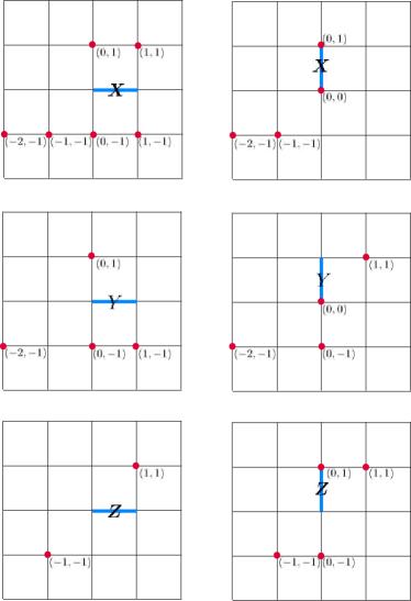
Figure 4: Syndromes of single-qubit errors for the $d=5$ bosonization.

3 Stabilizer codes and the Pauli module

This section discusses the stabilizer code formalism and the Pauli module representation via Laurent polynomials. The Laurent polynomial method is reviewed in Section. 3.1. Then, in Section. 3.2, we discuss bosonization with distance $d=3,4,5$ and the corresponding symplectic automorphisms. The searching algorithm for automorphisms is presented in Section. LABEL:sec:bosonization_search.

3.1 Review of the Laurent polynomial method for the Pauli algebra

We start by reviewing how any Pauli operator can be expressed as a vector over the Laurent polynomial ring $R={\mathbb{F}}_{2}[x,y,x^{-1},y^{-1}]$ as set out in Ref. [Haah_module_13]. First, we define $X_{12}$, $Z_{12}$, $X_{14}$, and $Z_{14}$ in Fig. 1 as column vectors: X_12= [1000],  Z_12= [0010],  X_14= [0100],  Z_14= [0001]. The Pauli $Y$ can be written as a vector which is a sum of corresponding vectors of $X$ and $Z$, such as Y_12=[1010]. We express the vector representation of the Pauli $Y$ operator on an edge $e$ as $XZ$ along the same edge. It is important to note that in this representation, we quotient out the phase factor ${\pm 1,\pm i}$ associated with Pauli operators. For instance, we equate ${Y,-Y,iY,-iY}$ with $Y$. Our primary focus is on the commutation and anti-commutation properties of Pauli operators; thus, quotienting out the phase factor ${\pm 1,\pm i}$ does not impede our calculations. In practical applications, the phase factor can be efficiently tracked, as demonstrated in the Gottesman-Knill theorem [gottesman1998heisenberg, aaronson2004improved].

All the other edges can be defined with the help of translation operators as follows. We use polynomials of $x$ and $y$ to represent translation in the $x$ and $y$ directions, respectively. For example, Z_78= y^2 [0010] = [00y^20],  X_58= x y [0100] = [0xy00]. More examples are included in Fig. 5.

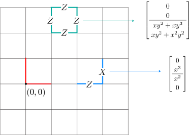
Figure 5: Examples of polynomial expressions for Pauli strings. The flux term (i.e., fermionic occupation) on a plaquette and the hopping term on an edge are both shown. The factors such as $x^{2}y^{2}$ and $x^{2}$ represent the locations of the operators relative to the origin.

Next, we introduce the antipode map that is an ${\mathbb{F}}_{2}$-linear map from $R$ to $R$ defined by x^a y^b →¯x^a y^b:=x^-a y^-b. To determine whether two Pauli operators represented by vectors $v_{1}$ and $v_{2}$ commute or anti-commute, we define the dot product as v_1 ⋅v_2 = ¯v_1^T Λv_2, where $T$ is the transpose operation on a matrix and Λ= [00100001-10000-100] is the matrix representation of the standard symplectic bilinear form. Notice that $-1$ is the same as $1$ because we are working over the ${\mathbb{Z}}_{2}$ field. For simplicity, we denote $\overline{(\cdots)}^{T}$ as $(\cdots)^{\dagger}$.

The two operators $v_{1}$ and $v_{2}$ commute if and only if the constant term of $v_{1}\cdot v_{2}$ is zero. For example, we calculate the dot products X_12 ⋅Z_12 = 1,  X_58 ⋅Z_14 = x^-1y^-1, and, therefore, $X_{12}$ and $Z_{12}$ anti-commute, whereas $X_{58}$ and $Z_{14}$ commute (their dot product only has a non-constant term $x^{-1}y^{-1}$). Furthermore, the physical meaning of $X_{58}\cdot Z_{14}=x^{-1}y^{-1}$ is that the shifting of $X_{58}$ in $-x$ and $-y$ directions by 1 step will anti-commute with $Z_{14}$. A translationally invariant stabilizer code forms an $R$-submodule $V$ such that v_1 ⋅v_2 = v_1^†Λv_2 = 0,  ∀v_1, v_2 ∈V. We now study the automorphisms $A$ of the symplectic form $\Lambda$: (A v_1) ⋅(A v_2) = v_1 ⋅v_2,  ∀v_1, v_2 ∈V. This is equivalent to $A^{\dagger}\Lambda A=\Lambda$. All matrices $A$ satisfying this equation form the symplectic group. We divide $A$ into $2\times 2$ blocks $A=\left[\begin{array}[]{c| c}a&b\\ \hline\cr c&d\end{array}\right]$, the automorphism condition becomes &[ a^†c^†b^†d^†] [ 0I-I0] [ abcd] = [ 0I-I0]

⇒ a^†d - c^†b = I,  a^†c = c^†a,  b^†d = d^†b. Examples of the automorphism $A$ are S&= [ I0cI], where c ∈Mat_2 [R] and c^†=c,
H=[ 0I-I0],
C= [ 1000r100001¯r0001], where r ∈R. $\textrm{Mat}_{2}[R]$ consists of all $2\times 2$ matrices with entries in $R={\mathbb{F}}_{2}[x,y,x^{-1},y^{-1}]$. The generators of the symplectic group are discussed in Appendix LABEL:sec:_elementary_automorphism. We have selected sixteen elementary automorphisms, denoted as $A_{1}$, $A_{2}$, $\cdots$, $A_{16}$, from the symplectic group. These automorphisms can be expressed by the conjugation of a unitary operator, i.e., the effect of the automorphism is P A⟶ U P U^†. The corresponding unitary circuits for the sixteen elementary automorphisms are illustrated in Fig. 6.

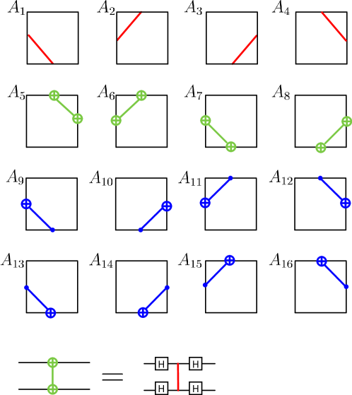
Figure 6: The circuit representations of sixteen elementary automorphisms. Red lines represent the $CZ$ gates, green lines represent the $H^{\otimes 2}(CZ)H^{\otimes 2}$ gates, and blue lines represent the $CNOT$ gates.

3.2 New stabilizer codes developed from automorphisms

First, we reformulate the original bosonization introduced in Section 2.1 and incorporate it into the Pauil module. For simplicity, we will write $x^{-1}$ and $y^{-1}$ as ${\overline{x}}$ and ${\overline{y}}$, respectively. The original hopping operators $U_{e}$ in Eq. (6) can be written as U_1= [100¯y], U_2= [01¯x0], where $U_{1}$ represents $U_{e}$ on the horizontal edge and $U_{2}$ represents $U_{e}$ on the vertical edge. The flux term $W_{f}$ in (7) is written as W= [001+y1+x]. The stabilizer $G_{v}$ in Eq. (9) corresponds to the vector G= [1+¯x1+¯y1+y1+x]. Now, we will apply automorphisms on these vectors to generate new stabilizer codes.

3.2.1 Automorphism for code distance $d=3$

We consider the simplest automorphism A_1= [ 1000010001101001], which modifies the Pauli operator $X_{e}$ as A_1 [1000] = [1001],  A_1 [0100] = [0110]. Pictorially, this is equivalent to X_e= {  . Notice that $Z_{e}$ is unchanged under this automorphism. This automorphism corrsponds to the Clifford circuit shown in Fig. 7.

Figure 7: Clifford circuit corresponding to automorphism $A_{1}$

Now we apply $A_{1}$ on the logical operators $U_{1}$, $U_{2}$, and $W$ and the stabilizer $G$: A_1 U_1 &= [1001+¯y],  A_1 U_2= [011+¯x0],
A