Using Answer Set Programming for HPC Dependency Solving

Abstract

Modern scientific software stacks have become extremely complex, using many programming models and libraries to exploit a growing variety of GPUs and accelerators. Package managers can mitigate this complexity using dependency solvers, but they are reaching their limits. Finding compatible dependency versions is NP-complete, and modeling the semantics of package compatibility modulo build-time options, GPU runtimes, flags, and other parameters is extremely difficult. Within this enormous configuration space, defining a “good” configuration is daunting.

We tackle this problem using Answer Set Programming (ASP), a declarative model for combinatorial search problems. We show, using the Spack package manager, that ASP programs can concisely express the compatibility rules of HPC software stacks and provide strong quality-of-solution guarantees. Using ASP, we can mix new builds with preinstalled binaries, and solver performance is acceptable even when considering tens of thousands of packages.

I Introduction

Managing dependencies for scientific software is notoriously difficult [1, 2, 3, 4]. Scientific software is typically built from source to achieve good performance, and configuring build systems, dependency versions, and compilers requires painstaking care. In the past decade, the modularity of HPC software has increased due to well known benefits such as separation of concerns, encapsulation, and code reuse. These enable application codes to leverage fast math libraries [5, 6, 7, 8] and GPU performance portability frameworks like RAJA [9] and Kokkos [10]. However, the cost of modularity is integration complexity: consumers of components must ensure that versions and other parameters are chosen correctly to ensure that all integrated components work together.

Package managers emerged in the mid-1990’s to mitigate the complexity of integrating software packages in Linux distributions. In the past decade, their use has exploded, particularly within language ecosystems like Python [11], Javascript [12], and Rust [13], but also within the HPC community. The HPC-centric package managers Spack [2] and EasyBuild [1] are now widely used for software deployment at HPC centers, and by developers and users installing their own software. The U.S. Exascale Computing Project (ECP) has adopted Spack as the distribution tool for its E4S [14] software stack (shown in Figure 1), which contains around 100 core software products and 500 required dependency packages.

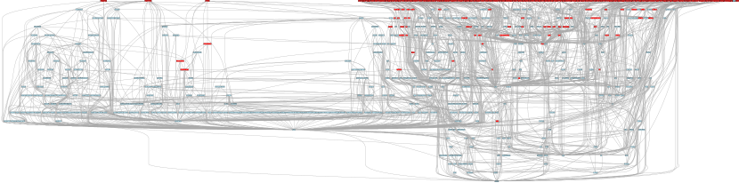
Figure 1: Graph of package dependencies in the Extreme Scale Scientific Software Stack (E4S) [14]. Around 100 core software products are shown in red, and the 500 required dependencies are blue. The precise number of packages required for a deployment of E4S is system-specific, depending on platform and hardware (e.g., NVIDIA, AMD GPUs).

Package managers address the integration problem in two main ways. Systems like EasyBuild and Nix [15, 16] rely on human effort, where maintainers develop fixed package configurations that define a common stack to be shared among users. To deviate from the stack, users must update all configuration files to ensure that versions and other parameters are consistent. More commonly, package managers like Spack provide flexibility for the end user by incorporating dependency solvers at their core. Users can request arbitrary versions, and packages declare constraints that bound the space of compatible configurations. The solver selects a set of versions and configuration parameters that satisfy the user’s requirements and package constraints.

Dependency solving is NP-complete, even for a “simple” configuration space with only packages and versions [17, 18]. Here, we focus on Spack’s dependency solver, known as the concretizer, which adds build options (variants), compilers, target microarchitectures, and dependency versions to make the space even larger. Most package managers use their own ad-hoc solver [19], and Spack is no different; it has historically used its own greedy algorithm. Heuristics were sufficient when there were only 245 packages [2], but now, Spack’s mainline repository contains over 6,000 packages, each with many constraints and options, and the original concretizer has begun to show its age. In particular, it lacks:

• Completeness: in a growing number of cases, it may not find a solution even though one exists; and

• Optimality: it provides no guarantees that it has found the “best” of all valid solutions according to any criteria.

An increasing number of package managers use Boolean satisfiability (SAT) solvers to resolve dependency constraints [19], which works well for version solving with a single optimization objective. With its added dimensions, Spack’s solver encodes a much larger configuration space and requires multi-objective optimization. Encoding these semantics in pure SAT is extremely complex. Instead, we have turned to Answer Set Programming (ASP) [20, 21], a declarative model that allows us to encode dependency semantics in a first-order, Prolog-like syntax. ASP solvers reduce first-order logic programs to SAT and optimization, and they guarantee both complete and optimal solutions. Unlike Prolog, they are also guaranteed to terminate. ASP encodings are non-trivial, and this paper presents the first dependency solver capable of making strong guarantees for the full generality of HPC dependency semantics. Specifically, our contributions are:

1. A general mapping of Spack’s DSL, compatibility semantics, and optimization rules to ASP;

2. A technique to optimize for reuse of existing builds in combinatorial package solves;

3. An ASP solver implementation in Spack that enables complete and optimal solutions; and

4. An evaluation of our system’s performance on the E4S repository with tens of thousands of packages.

Together, these contributions allow us to replace Spack’s original concretizer with a complete, optimizing solver, written in around 800 lines of declarative ASP. This represents a leap forward in capability, maintainability, and extensibility to the ever-increasing complexity of HPC software.

II Package Managers

The idea of “software release management” for integrated sets of packages dates back to a 1997 paper from Van der Hoek et al. [22], and the first Linux package managers emerged around the same time [23, 24]. Since then, the number and complexity of software packages has grown enormously, as have the use cases for package managers.

II-A Single-prefix Package Managers

Package managers such as RPM, Yum, and APT [25, 26, 27] are used to manage the system packages of most Linux distributions. These tools focus on managing one software stack, built with one compiler, which works well for system software and drivers that underlie all software on the system. They are designed so that software can be upgraded in place for bug fixes and security updates. All software goes in to a single prefix, e.g., /usr, and for this reason, only one version of any package can be installed at a time. Upgrades are prioritized over reproducibility, and users do not have great flexibility over precise package versions and configurations.

Even in this limited package/version configuration space, dependency solving is NP-complete [17, 28] because any two non-overlapping version constraints can cause a conflict. The Common Upgradeability Description Format (CUDF) attempts to standardize an interface for external package solvers [29, 30] and has enabled many encodings of the single-prefix upgrade problem: Mixed-Integer Linear Programming, Boolean Optimization, and Answer Set Programming [31, 32, 33, 34]. Most modern package solvers still use ad-hoc implementations instead of a common external solver [19].

II-B Language Package Managers

Most modern language implementations also include their own package managers [12, 11, 13, 35]. The solver requirements for language package managers are different from those in a Linux distribution; they typically allow multiple versions of the same package to be installed to support developer workflows and reproducibility. Conflicts can arise, as most language module systems do not support linking multiple versions of one package into a single executable. Javascript is a notable exception to this. Language package managers still solve only for package names and versions, ignoring compilers, build options, targets and other options that expand the solution space. Most language package managers implement their own ad-hoc solvers. Historically, these solvers were not complete, as implementing a performant SAT solver in all but the lowest-level languages is quite difficult. However, there has been a recent trend towards complete solvers [36, 35] as complexity of language ecosystems has grown. These systems do not support optimization beyond selecting recent versions [19].

II-C Functional and HPC Package Managers

So-called “functional” package managers like Nix [15, 16] and Guix [37] allow users to install arbitrarily many configurations of a given package. Like many HPC deployments, they install each configuration to a unique prefix, but instead of a human-readable name, they ensure that each installation gets a unique prefix by using a hash of the bits of the installation itself. These systems do not use solvers to resolve dependencies. Rather, they have very little conditional logic and rely on the specific package recipes in a repository. As mentioned, EasyBuild [1] is similar in this regard, as it allows multiple configurations of packages by duplicating package recipes and adhering to a strict naming convention to differentiate different installations. In all of these systems, users must modify code in package recipes to change the way dependencies are resolved.

III Spack

Spack [2] is a package manager designed to support High Performance Computing (HPC). Like functional package managers, Spack installs packages in separate prefixes to allow arbitrarily many installations to coexist. This enables users to build many different variants of a package, e.g., with different compilers, different MPI implementations, different flags, or with combinations of all three of these parameters. This greatly expands the space of possible build configurations.

At a high level, Spack can be broken down into three primary components. The spec syntax allows users to easily specify and constrain builds on the command line. The package domain-specific language (DSL) expresses parameterized build recipes for software packages, and the concretizer is Spack’s dependency solver. The concretizer combines abstract (i.e., underspecified) spec constraints from the user and from packages, and it produces a concrete, or fully specified package spec that can be installed. We provide an overview of these pieces here but full details are in the original paper [2].

III-A Spec Syntax

Spack calls its internal dependency graphs “specs” because they specify parameters of a software installation along with those of its dependencies. Specs are directed acyclic graphs where nodes are packages and edges are dependency relationships. The “spec syntax” is a shorthand for expressing constraints on these graphs. Each node of the graph has parameters, including 1. the package name; 2. the version to build; 3. variants (compile-time build options); 4. the compiler to build with and its version; 5. compiler flags; 6. the target operating system; 7. the target microarchitecture; and 8. the package installation’s dependencies.

Sigil	Examples	Meaning
%	hdf5%gcc	Use a particular compiler
@	hdf5@1.10.2	Require version(s)
	hdf5%gcc@10.3.1	Require compiler version(s)
+	hdf5+mpi	Enable (+)/disable (~) variant
~	hdf5~mpi
key=value	hdf5 mpi=true	Require a particular variant or build target value
	hdf5 api=default
	hdf5 target=skylake

TABLE I: Spec sigils in Spack

The spec syntax in Spack allows users to specify preferences within this combinatorial build space. In the simplest case, a user might want to build a particular package without any concern for its configuration. In this case they would write:

⬇

spack install hdf5

Spack will install hdf5 without any particular customization. Table I shows examples of sigils that can be used to specify specific constraints on specs, including any of the attributes listed above. The spec syntax is fully recursive, in that users can specify constraints on dependencies using the ^ (“depends on”) sigil. For example, the spec below:

⬇

hdf5@1.10.2 ^zlib

means “any possible build of the package hdf5 at version 1.10.2 that depends on a build of the package zlib built with the gcc compiler and a build of the package cmake built to target the aarch64 architecture”. While users could completely constrain a build via the spec syntax, in practice they only care about a comparatively small set of constraints, and they rely on concretization to select values for unspecified parameters. We refer to a portion of the build space in Spack as an “abstract spec”, and a fully specified build as a “concrete spec”.

III-B Package DSL

⬇

# This is the class name for the package ‘example‘

class Example(Package):

”””Example depends on zlib, mpi, and optionally bzip2”””

\parversion(”1.1.0”)

version(”1.0.0”)

\parvariant(”bzip”, default=True, description=”enable bzip”)

\par# Depends on bzip2 or later when bzip is enabled

depends_on(”bzip2@1.0.7:”, when=”+bzip”)

depends_on(”zlib”) # depends on zlib

# Newer versions require newer versions of zlib

depends_on(”zlib@1.2.8:”, when=”@1.1.0:”)

\par# Depends on *some* MPI implementation

depends_on(”mpi”)

\par# Known failure when building with intel compilers

conflicts(”# Does not support architectures derived from ARM64

conflicts(”target=aarch64:”)

\pardef install(self, spec, prefix):

# Translate spec into arguments to build system

config_args = [’–with-zlib=\parif ’bzip2’ in spec:

bz_arg = ’–with-bzip=else:

bz_arg = ’–without-bzip’

config_args.append(bz_arg)

\par# Run the build

configure(*config_args)

make()

make(’install’)

Figure 2: A package.py file written in Spack’s embedded DSL.

Figure 2 shows Spack’s package DSL. Unlike many systems, a package in Spack is a parameterized Python class. There is one package recipe for each package, and it is instantiated for each concrete spec that Spack builds. The install() function on line 24 takes a fully concrete spec as one of its parameters, and its job is to install that particular configuration of the example package into the specified prefix.

The install instructions on lines 24-37 do the work of the build, but more interesting for this paper are the metadata directives on lines 5-22. This package has two possible versions, 1.0.0 and 1.1.0. It has one build option, or “variant”, called bzip that enables the dependency on bzip2. Its dependency on zlib is dependent on its version. Conditions like these are specified using when clauses within directives. It has some conflicts—conditions under which it is known not to build successfully. Dependency constraints, conflicts, and when clauses are all specified concisely using the spec syntax. The dependency on mpi on line 17 is special. Spack provides support for packages that are source-compatible (API-compatible), like MPI. There is no concrete mpi package in Spack, rather there are several mpi providers, like mpich, openmpi, etc. This package can be instantiated with any of these MPI providers. We thus call mpi a“virtual dependency”. blas and lapack are two other common examples in HPC.

III-C Concretization

Spack can build the example package in Figure 2 in many different ways. The metadata in the package DSL exposes a combinatorial build configuration space, and it is the concretizer’s job to select a configuration. The concretizer is Spack’s dependency solver, so called because it converts partially constrained abstract specs to fully constrained concrete specs that can be built when combined with installation methods in the package DSL. There are three primary inputs to concretization in Spack: specs on the command line, constraints from the package DSL, and additional preferences from user configuration files. Without loss of generality, we consider only the first two here.

III-C1 Validity

On a conceptual level, we can think of the concretizer as accomplishing two tasks. First, it determines the set of packages needed in the spec DAG. Second, it fills in any missing nodal parameters (enumerated in Section III-A). Every decision made by the concretizer must consider constraints from all the input sources; any unsatisfied constraints imply an invalid solution. We say a solution is valid if and only if:

• all virtuals are replaced with concrete dependencies;

• all dependencies are resolved;

• all node parameters have been assigned values; and

• all input constraints are satisfied.

III-C2 Completeness

The original Spack concretizer used a greedy, fixed-point algorithm. The issue with this algorithm (and all greedy algorithms) is that it only made local decisions about dependencies and node parameters, and it could not backtrack to undo decisions that it made. A solver is complete if it finds a solution when one exists; this property of the original concretizer made it incomplete.

Consider our package example from Section III-B, we will concretize the abstract spec:

⬇

example@1.0.0 ^zlib@1.2.11

We will assume for the moment that neither zlib nor bzip2 have any additional dependencies. The solver needs to consider contraints from package files and from the abstract spec supplied on the command line. Here, those constraints are:

• example@1.0.0 from the abstract spec: “example v1.0.0”

• bzip2@1.0.7: from example: “bzip2 v1.0.7 or higher”

• zlib@1.2.11 from abstract spec: “zlib version 1.2.11”

• mpi from example: “any MPI implementation”

The original concretizer would simply proceed until all decisions had been made, stopping at the first conflict it found with any prior decision. The resulting concrete spec might be:

⬇

example@1.0.0+bzip^bzip2@1.0.8+pic^zlib@1.2.11+pic^mpich@3.1 pmi=pmix

Here, all dependencies are expanded, all virtual packages have been replaced, all node parameters (variants, compilers, targets, etc.) have been assigned and no constraints are violated. Decisions regarding node attributes not specified in the abstract spec nor in the package constraints were made from defaults. But, imagine that mpich had a conflict with bzip2@1.0.7. In our example, we were lucky that the concretizer selected bzip2@1.0.8 to satisfy the constraint bzip2@1.0.7: (recall that means bzip2 at version 1.0.7 or higher). Had the default choice been bzip2@1.0.7, there would have been no way for the algorithm to backtrack, and it would fail with no solution.

III-C3 Optimality

There are usually many valid solutions to concretization problems, but users prefer some solutions over others. For a fresh installation, users generally prefer the newest version of a package. They prefer certain defaults for build options and variants, and HPC users tend to prefer specific microarchitecture targets with vector instructions, e.g., skylake or cascadelake with AVX-512 support vs. generic x86_64. We say a solver is optimal when it can find the best valid solution according to some set of formal criteria. Since the original concretizer was not complete, it also could not be optimal, as it could never consider all possibilities. Note that this definition of optimality does not refer to the performance of built binaries, though it may be related depending on the criteria chosen (we discuss this in later sections).

In addition to these issues, the original concretizer was implemented directly on the dependency graph structure in memory. Any new semantics had to be implemented with complex graph algorithms, and graph nodes and edges had to be configured and updated manually. This process was error-prone and limited the speed of development and the complexity of the semantics that could be considered.

IV Answer Set Programming

The concretization problem is essentially a combinatorial search problem. While many package managers use homegrown SAT solvers for this type of problem, encoding the complexity of our domain in pure Boolean SAT would be extremely tedious. To manage the complexity, we leverage Answer Set Programming (ASP), a form of declarative programming that allows us to formally specify our semantics in first-order logic with variables and quantification, in addition to Boolean operators. The input language for ASP is similar to Prolog [38]. Unlike Prolog, ASP has no operational semantics and is not Turing-complete. Rather, ASP converts first-order logic programs (with quantifiers and variables) to propositional programs (with no variables). It then uses techniques borrowed from SAT solvers to find solutions. One major benefit of this approach is that unlike Prolog, ASP programs are guaranteed to terminate.

In the remainder of this section, we illustrate how ASP can simplify the specification and maintenance of our concretization algorithm while also affording strong guarantees than we can implement ourselves with simple heuristics.

IV-A ASP Syntax

ASP programs are comprised of “terms”, which can be Boolean atoms or a functions whose arguments may also be terms. A term followed by a period (.) is called a “fact”. The following is a simple program comprised entirely of facts:

⬇

optimize_for_reuse.

node(”hdf5”).

depends_on(”hdf5”, ”mpi”).

Note that these functions are not imperative; rather this snippet can be ready roughly as “optimize_for_reuse is enabled. A node called hdf5 exists. hdf5 depends on mpi.”

In addition to facts, ASP programs contain rules, which can derive additional facts. An ASP rule has a head and a body, separated by :-. The :- can be read as “if” — the head (left side) is true if the body (right side) is true. Terms in the body of a rule can also be preceded by the keyword “not” to imply the head based on their negation. Logical “and” is represented by a comma in the rule body, and “or” is represented by repeating the head with a different rule body.

ASP programs can contain variables, represented by capitalized words. Variables are scoped to the rule or fact in which they appear; the variable Package may be used in unrelated rules without any scoping issues. Rules are instantiated with all possible substitutions for variables. For example:

⬇

node(”hdf5”).

depends_on(”hdf5”, ”mpi”).

node(Dependency) :-

node(Package), depends_on(Package, Dependency).

The rule here translates roughly to “If a package is in the graph and it depends on another package, that package must be in the graph”, and the rule in the program above will derive the fact node("mpi") when it is instantiated with node("hdf5") and depends_on("hdf5", "mpi"). This is the essence of how we model dependencies in ASP.

IV-B Integrity Constraints and Choices

Two additional types of rules are important to understand the power of ASP: integrity constraints and choice rules. Integrity constraints allow the programmer to rule out swathes of the answer set space by specifying conditions not to allow. In ASP, these are represented by a headless rule:

⬇

node(”hdf5”).

depends_on(”hdf5”, ”mpi”).

node(Dependency) :-

node(Package), depends_on(Package, Dependency).

:- depends_on(Package, Package).

This constraint says “a package cannot depend on itself”.

IV-C Choice Rules

Choice rules give the solver freedom to choose from possible options. A choice rule is (optionally) constrained on either side to specify the minimum (left) and maximum (right) number of choices the solver can select.

⬇

node(”hdf5”).

depends_on(”hdf5”, ”mpi”).

node(Dependency) :-

node(Package), depends_on(Package, Dependency).

:- depends_on(Package, Package).

\parpossible_version(”hdf5”, ”1.13.1”).

possible_version(”hdf5”, ”1.12.1”).

1 { version(P, V) : possible_version(P, V) } 1 :-

node(P).

The choice rule on the last line means “If a package is in the graph, assign it exactly one of its possible versions.” The $\{a:b\}$ syntax here has the same meaning as in formal set theory; it denotes the set of all $a$ such that $b$ is true. The numerals on either side of the choice rule are cardinality constraints; they specify lower and upper bounds on the size of the set. Choice rules are similar to guessing; they give the solver options for paths to explore next.

IV-D Optimization

In addition to constraints on the solution space, ASP allows optimization criteria. Optimization criteria allow the solver to return a single answer set from the among all valid answer sets, and they guarantee that the chosen answer set minimizes or maximizes one or many criteria. There are often many valid solutions to a dependency resolution query, but only the optimal solution is relevant once we find it.

⬇

node(”hdf5”).

depends_on(”hdf5”, ”mpi”).

node(Dependency) :-

node(Package), depends_on(Package, Dependency).

:- depends_on(Package, Package).

\parpossible_version(”hdf5”, ”1.13.1”, 0).

possible_version(”hdf5”, ”1.12.1”, 1).

\par1 { version(P, V) : possible_version(P, V) } 1 :-

node(P).

\parversion_weight(P, V, Weight) :-

possible_version(P, V, Weight).

#minimize{ W@3,P,V : version_weight(P, V, W)}.

This optimization constraint says “I prefer (at priority 3) solutions that minimize the sum of the weights (W) of the package (P) versions (V), for all packages and versions.” A detailed discussion of the syntax for optimization is beyond the scope of this paper; it suffices to know that multi-objective optimization across a variety of criteria is possible in ASP.

This small and very incomplete program already shows the power of ASP. In a SAT solver, the programmer would need to write out explicitly the rule for deriving dependency nodes from dependent nodes for every possible pair of packages. Even worse, our choice rule for selecting versions would need to be written out for every combination of package and version, along with a combinatorial set of clauses ensuring that for any versions $a_{1},...,a_{n}$, exactly one $a_{i}$ is set but not any $a_{j}$ for all $i\neq{j}$. ASP makes this much simpler.

IV-E Grounding and Solving

ASP solvers search the input program for stable models, also known as answer sets. An answer set is a set of true atoms for which every rule in the input program is idempotent. It is similar to a fixed point, or the solution to a system of (Boolean) equations. When ASP first emerged in the late 1990’s, it used custom solvers. However, the problem domain of ASP is NP-complete, and the 2000’s brought great advances [39] in solving the canonical NP-complete problem: Boolean satisfiability (SAT). Modern ASP solvers exploit high-performance techniques developed in the SAT community [20].

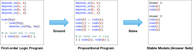
Figure 3: Grounding and solving in Answer Set Programming.

The ASP input language, with first-order rules and variables, is very expressive, but SAT solvers deal with propositional logic programs that have no variables. A logic expression that has no variables is called a ground term, and grounding is the process of converting a first-order ASP rules to a set of ground rules. We call these the “ground instances” of the rule.

Figure 3 shows the grounding and solving process at a very high level. On the left is an ASP program with four facts, one first-order rule, and a choice rule that says we must choose at least one of node(a) or node(b) to be in the solution. Grounding this program instantiates the first-order rule with all possible ground atoms that can be substituted into its body. The ground instances are built from input depends_on() facts, node(a) and node(b) from the choice rule, as well as node(c) and node(d), which appear in the heads of ground rules instantiated from node(a) and node(b). Note that the ground instances are simplified—they omit depends_on() terms because these are facts in the input, and therefore always true. Grounders perform many such optimizations to prune the propositional program and to make the solver more efficient.

Propositional logic programs can be reduced to SAT and solved using techniques similar to those used in modern SAT solvers [20]. For this program, there are two stable models: one with only node(b) and node(d) (when only node(b) is selected by the choice rule) and one with all four nodes (when only node(a) or both node(a) and node(b) are selected). It is easy to see from this result how we could read in these lists of nodes and construct graphs from them. This how Spack reads solutions in from the solver.

We use the popular clingo [40] system, which includes a grounder (gringo) and a solver (clasp). The search algorithm used in clasp traces its roots to the well known Davis–Putnam–Logemann–Loveland (DPLL) algorithm [41, 42], but uses modern extensions like Conflict-Driven Clause Learning (CDCL) for high performance [39]. clasp can also do MaxSAT-style optimization. The internals of clingo are beyond the scope of this paper, but is important to understand that because it effectively performs an exhaustive combinatorial search, it guarantees completeness and optimality. There are no inputs for which clingo will return a false negative (claim compatible rules are incompatible) and solutions are guaranteed to be optimal according to provided criteria.

V Modeling Software Dependencies with ASP

At a high-level, using clingo, our concretizer combines:

1. Many facts characterizing the problem instance;

2. A small logic program encoding the rules and constraints of the software model; and

3. Optimization criteria that define an optimal model.

The facts are always generated starting from one or more root specs, and they account for metadata from all package recipes of possible dependencies, as well as the current state of Spack in terms of configuration and installed software. This directive:

⬇

version(’1.2.11’, sha256=’ah45rstgef…’)

in zlib’s recipe is translated to the following fact:

⬇

version_declared(”zlib”, ”1.2.11”, 0).

where 0 is the preference weight of this version. Similarly:

⬇

zlib@1.2.11

generates the following three facts:

⬇

root(”zlib”).

node(”zlib”).

version_satisfies(”zlib”,”1.2.11”).

stating that zlib is a root node and should satisfy a version requirement. A typical solve has around $10k-100k$ facts that encode dependencies, variants, preferences, etc.

The logic program encodes the software model used by Spack and only contains first-order rules, integrity constraints, and optimization objectives. The declarative nature of ASP makes it easy to enforce certain properties on the solution. For instance, these three lines ensure that we never have a cyclic dependency in a DAG:

⬇

path(A, B) :- depends_on(A, B).

path(A, C) :- path(A, B), depends_on(B, C).

:- path(A, B), path(B, A).

The first rule is the base case: if A depends on B there is a path from A to B. The second rule defines paths to transitive dependencies recursively: if there is a path from A to B and B depends on C, there is a path from A to C. The final line is an integrity constraint banning paths from A to B and paths from B to A from occurring together in a solution.

To give a rough idea of the compactness and expressiveness of the ASP encoding, the entire logic program for the software model described here is around $800$ lines. The concretization process is straightforward to follow conceptually within Spack:

1. Generate facts for all possible dependencies/installs ;

2. Send logic program and facts to the solver;

3. Retrieve the best stable model; and

4. Build an optimal concrete DAG from the model.

The word “optimal” is emphasized since, while rules and integrity constraints fully determine if a solution is valid, we need optimization targets to select one of the many possible solutions in a way that fits user’s expectations.

A good example to illustrate this point is target selection for DAG nodes. In Spack each node being built has a target microarchitecture associated with it, and we want to use the best target possible while respecting the constraints coming from the compiler (for example, gcc@4.8.3 cannot generate optimized instructions for skylake processors). Previously this required some complicated logic mixed with the rest of the solve. The introduction of clingo greatly simplified the problem definition. A cardinality constraint is used to express that the solver must choose one and only one target per node:

⬇

1 { node_target(Package, Target) : target(Target) } 1

:- node(Package).

A user’s choice will force the target of a node:

⬇

node_target(P, T) :- node(P), node_target_set(P, T).

An integrity constraint prevents choosing targets not supported by the chosen compiler:

⬇

:- node_target(P, T),

not compiler_supports_target(C, V, T),

node_compiler(P, C),

node_compiler_version(P, C, V).

These three statements fully describe the characteristics of a valid solution. To pick the optimal solution we also weight the possible targets (the lower the weight, the best the target) and optimize over the sum of target weights:

⬇

node_target_weight(P, W) :-

node(P), node_target(P, T), target_weight(T, W).

#minimize { W@5,P : node_target_weight(P, W) }.

V-A Generalized Condition Handling

A unique feature of Spack, as a package manager, is that it optimizes not only for versions but for many other aspects of the build, e.g., which compiler to use, which microarchitecture to target, etc. The DSL used for package recipes reflects this complexity by having multiple directives to declare properties or constraints on software packages, as seen in Section III.

One interesting abstraction that we observed while coding the ASP logic program is that each of these directives can be seen as a way to impose additional constraints on the solution, conditional on other constraints being met. For instance, the following directive in a package:

⬇

depends_on(’hdf5+mpi’, when=’+mpi’)

means that, if the spec has the mpi variant turned on, then it depends on hdf5+mpi. Similarly:

⬇

provides(’lapack’, when=’@12.0:’)

means that a package provides the LAPACK API if its version is $12.0$ or greater. This property allowed to encode all the directives as generalized conditions, where most of the semantics is encoded abstractly in a few lines of the logic program.

Getting back to a simple example, the snippet below:

⬇

class H5utils(AutotoolsPackage):

depends_on(’png@1.6.0:’, when=’+png’)

is translated to the following facts:

⬇

condition(153).

condition_requirement(153, ”node”, ”h5utils”).

condition_requirement(153, ”variant_value”, ”h5utils”, ”png”, ”true”).

imposed_constraint(153, ”version_satisfies”, ”libpng”, ”1.6.0:”).

dependency_condition(153, ”h5utils”, ”libpng”).

when setting up the problem to be solved by clingo. The important points to note are that:

• Each directive is associated with a unique global ID.

• Constraints are either “requirement” or “imposed”.

• Different type of conditions have different semantics

The code to trigger and impose general conditions in the logic program is surprisingly simple to read. ASP conditional rules allow us to effectively build new rules from input facts:

⬇

condition_holds(ID) :-

condition(ID);

attr(N, A1) : condition_requirement(ID, N, A1);

attr(N, A1, A2): condition_requirement(ID, N, A1, A2).

based on their number of arguments, or arity. Other rules:

⬇

attr(N, A1) :- condition_holds(ID),

imposed_constraint(ID, N, A1).

attr(N, A1, A2) :- condition_holds(ID),

imposed_constraint(ID, N, A1, A2).

enforce the imposed constraints when a condition holds.

V-B Usability Improvements due to clingo

As mentioned, the original concretizer was incomplete and could fail to find a solution when one exists. Users would work around such false negatives by overconstraining problematic specs, to help the solver find the right answer. This could become very tedious.

V-B1 Conditional Dependencies

A prominent example of this behavior is with packages having dependencies conditional to a variant being set to a non-default value. Let’s take for instance hpctoolkit, which has the following directives:

⬇

class Hpctoolkit(AutotoolsPackage):

variant(’mpi’, default=False, description=’…’)

depends_on(’mpi’, when=’+mpi’)

Trying to use the old algorithm to concretize hpctoolkit ^mpich fails like this:

⬇

$ spack spec hpctoolkit ^mpich

Input spec

——————————–

hpctoolkit

^mpich

\parConcretized

——————————–

==> Error: Package hpctoolkit does not depend on mpich

since the greedy algorithm would set variant values before descending to dependencies. Since no value is specified for the mpi variant, the value chosen is false (the default) which leads to hpctoolkit having no dependency on mpi. The workaround required users to understand the conditional dependency and write hpctoolkit+mpi ^mpich to concretize successfully. With clingo, the concretizer simply finds the correct value for the mpi variant, as setting it is the only way for mpich to be part of the solution.

V-B2 Conflicts in Packages

Before using clingo, conflicts in packages were only used to validate a solution computed by the greedy-algorithm. If the solution matched any conflict, Spack would have errored and hinted the user on how to overconstrain the initial spec to help concretization. With ASP, conflicts are generalized as constraints during the solve and Spack no longer needs to ask the user to be more specific.

V-B3 Specialization on Providers of Virtual Packages

Using clingo also enabled more complex use cases e.g. imposing constraints on specific virtual package providers. A simple example of that is given by the berkeleygw package, which has the following directives:

⬇

class Berkeleygw(MakefilePackage):

variant(’openmp’, default=True)

depends_on(’lapack’)

depends_on(’openblas threads=openmp’,

when=’+openmp ^openblas’)

The last directive forces openblas to have openmp support if berkeleygw has openmp support and openblas has been chosen as a provider for the mandatory lapack virtual dependency. Conditional constraints of that complexity could not be expressed before, because the solver would select defaults for openblas before evaluating the conditional constraint on it.

V-C Optimization Criteria

Priority	Criterion (to be minimized)
1	Deprecated versions used
2	Version oldness (roots)
3	Non-default variant values (roots)
4	Non-preferred providers (roots)
5	Unused default variant values (roots)
6	Non-default variant values (non-roots)
7	Non-preferred providers (non-roots)
8	Compiler mismatches
9	OS mismatches
10	Non-preferred OS’s
11	Version oldness (non-roots)
12	Unused default variant values (non-roots)
13	Non-preferred compilers
14	Target mismatches
15	Non-preferred targets

TABLE II: Spack’s optimization criteria in order of priority.

The conditional logic presented here provides a great deal of flexibility, but with this flexibility we also need to have sensible defaults for users who do not want to think about all of the degrees of freedom Spack allows. Coming up with “intuitive” solutions to the package configuration problem is surprisingly difficult, but we have developed the list of optimization criteria in Figure II based on our experiences interacting with users and facilities. There are currently 15 criteria we consult at to pick the best valid solution for a package DAG. All are minimization criteria, and they are evaluated in lexicographic order, i.e., the highest priority criteria are optimized first, then the next highest, and so on.

Our top priority (1) is to avoid software versions that have been deprecated due to security concerns or bugs. Priorities 2-5 choose the newest versions and default variant values and providers for roots in the DAG. We prioritize versions first, then virtual providers (e.g., the user’s preferred MPI), then default variant values. After root configuration, we prioritize non-root configuration (6-7, 11-12). Preferences flow downward in the DAG via dependency relationships, and if a root demands a particular version of a dependency, the dependency’s preference should not be able to override this. Ideally, we would enforce strict DAG precedence on preferences (i.e., every node’s preference would dominate those of its dependencies), but we have seen performance penalties when attempting to track the relative depths of all nodes, so we settle for a two-level hierarchy of roots and non-roots. We try to enforce consistency in the resolved graph by minimizing “mismatches” (8-9, 14)—these criteria ensure that neighboring nodes are assigned consistent compilers, OS’s and targets unless otherwise requested. We model preferred compilers, targets, and OS’s for non-roots at lower priority than mismatches, so that dependencies inherit these properties from their dependents unless set explicitly by the user. All preferred versions, compilers, OS’s, targets, etc. can be overridden through configuration in Spack.

Spack’s optimization criteria are unique among dependency solvers in that many of them are simply not modeled by other systems. In a typical Linux distribution like Debian, target and toolchain compatibility are not modeled—they are uniform across the DAG. If we look at aspcud [34], an ASP solver plugin for Debian’s APT, we see that there are around 6 optimization criteria, all to do with versions and version preferences, far fewer than the 15 criteria modeled here.

VI Reusing Already Built Packages

While Spack is primarily a package manager installing software from sources, the ability to reuse already built software and mix it seamlessly with source builds has been a critical request from the community for several years.

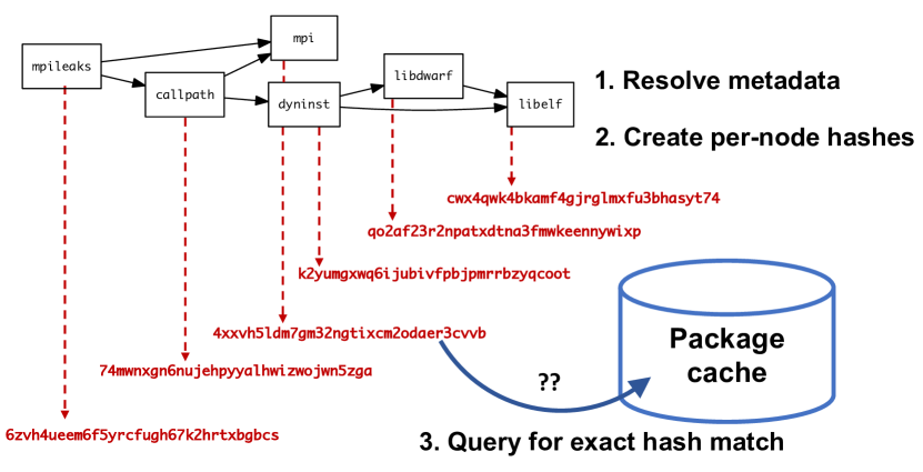
Figure 4: Hash-based reuse in the original Spack concretizer.

Functional packaging systems, including Spack with the old concretizer, reuse builds via metadata hashes. This mechanism relies on the fact that, when an installation graph is concretized, each node in the DAG is given a unique hash, as shown in Figure 4. Unless the user was explicit, Spack only reused packages if their hashes matched exactly. Small configuration changes could easily result in little or no reuse.

A more effective way to approach software reuse can be achieved by leveraging the “Generalized Condition Handling” logic described in Section V-A. First, all the metadata from installed packages can be encoded into facts:

⬇

installed_hash(”zlib”,”7fatd…”).

imposed_constraint(”7fatd…”,”node”,”zlib”).

imposed_constraint(”7fatd…”,”version”,”zlib”,”1.2.11”).

imposed_constraint(”7fatd…”,”node_platform”,”zlib”,”linux”).

imposed_constraint(”7fatd…”,”node_os”,”zlib”,”ubuntu20.04”).

imposed_constraint(”7fatd…”,”node_target”,”zlib”,”icelake”).

…

The encoding is based on imposed_constraint, but the constraint ID is the hash associated with the installed package. To minimize the number of builds from source, the solver is allowed to choose a hash to resolve any package:

⬇

{hash(P, Hash) : installed_hash(P, Hash)} 1 :- node(P).

It imposes all constraints associated with chosen hashes:

⬇

impose(Hash) :- hash(P, Hash).

And number of builds (packages without a hash) is minimized:

⬇

build(P) :- not hash(P, _), node(P).

#minimize { 1@100,P : build(P) }.

This is a remarkably simple encoding for a complex constraint problem that cannot be solved with the prior greedy concretizer. However, the devil is in the details. Minimizing builds can have two effects—it can cause the concretizer to prefer an existing installation over building a new version of a package, but if set as the highest optimization priority, it also causes the concretizer to configure newly built packages in any way that minimizes dependencies. Generally, though, users expect new builds to use regular defaults—i.e., most recent version, preferred variants, etc. As an illustrative example, building cmake with these objectives will build without networking capabilities, because it omits openssl and its dependencies from the graph!

Our solution is to split the optimization criteria into two sets of identical “buckets”, one for installed software and one for software to be built, and order their priorities:

1. Minimize all objectives for software to be built

2. Then, minimize the number of builds

3. Minimize all objectives for already built software

This is actually fairly simple to encode in ASP:

⬇

build_priority(P, 200) :- build(P), node(P).

build_priority(P, 0) :- not build(P), node(P).

#minimize{

W@2+Priority,P

: version_weight(P, W), build_priority(P, Priority)

}.

For each criterion defined in Table II, we include a #minimize statement like the one above. It contributes a version weight W for each package P in the graph to bucket number 2 + Priority. Priority is 200 if the package needs to be built, but it is zero if the package is already installed. The structure of these buckets for a scenario with three criteria is shown in Figure 5. Buckets are ordered by priority from high to low, and the three per-criterion buckets for built packages have priorities 203, 202, and 201. In the middle, at priority 100, is the total number of builds, and below it are all the original criteria with their original numbers: 3, 2, and 1. This vector is computed for each model and compared lexicographically to determine the “best” one.

If we ensure that all of our optimization criteria are minimizing, i.e., that the “best” value for any criterion is zero, then any scenario where a package must be built will still be worse than one where it is reused. Even if all criteria are minimized for built packages, the number of builds will still be greater than zero, making the build scenario worse, because number of builds has higher priority. This allows Spack to pick the best version available from what is installed without adversely affecting the choice of defaults for built packages. Spack will prefer to build the default configuration of a package that it has to build, even if that means building more packages. However, if some installed package can satisfy a dependency requirement, Spack will prefer to reuse it.

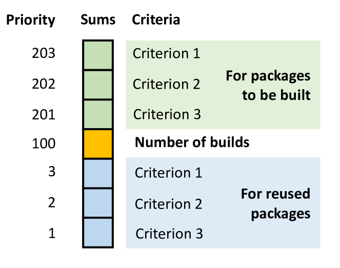
Figure 5: Vector of accumulated weights of optimization criteria. Contributions to each criterion’s objective are divided into two buckets: a higher priority bucket if the package is to be built, and a lower priority bucket if the package is already installed. Objective vectors are compared lexicographically.

The benefits of reusing packages are clear. Figure 6a shows a concretization relying on purely hash-based software reuse. We can see that no match was found and 20 installations need to be performed from source. In Figure 6b we show the same concretization with the reuse logic turned on. In this case 16 installed packages can be reused and only 4 need to be built. As described above, reuse takes priority over the defaults for already installed software, allowing Spack to reuse cmake 3.21.1 even though the preferred version for a new build is 3.21.4. This can save users considerable time.

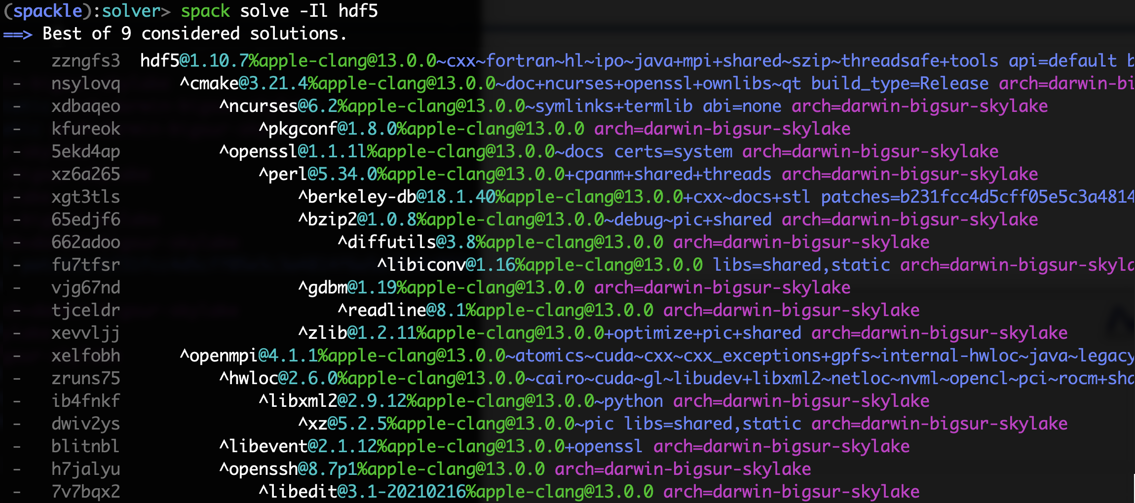
(a)

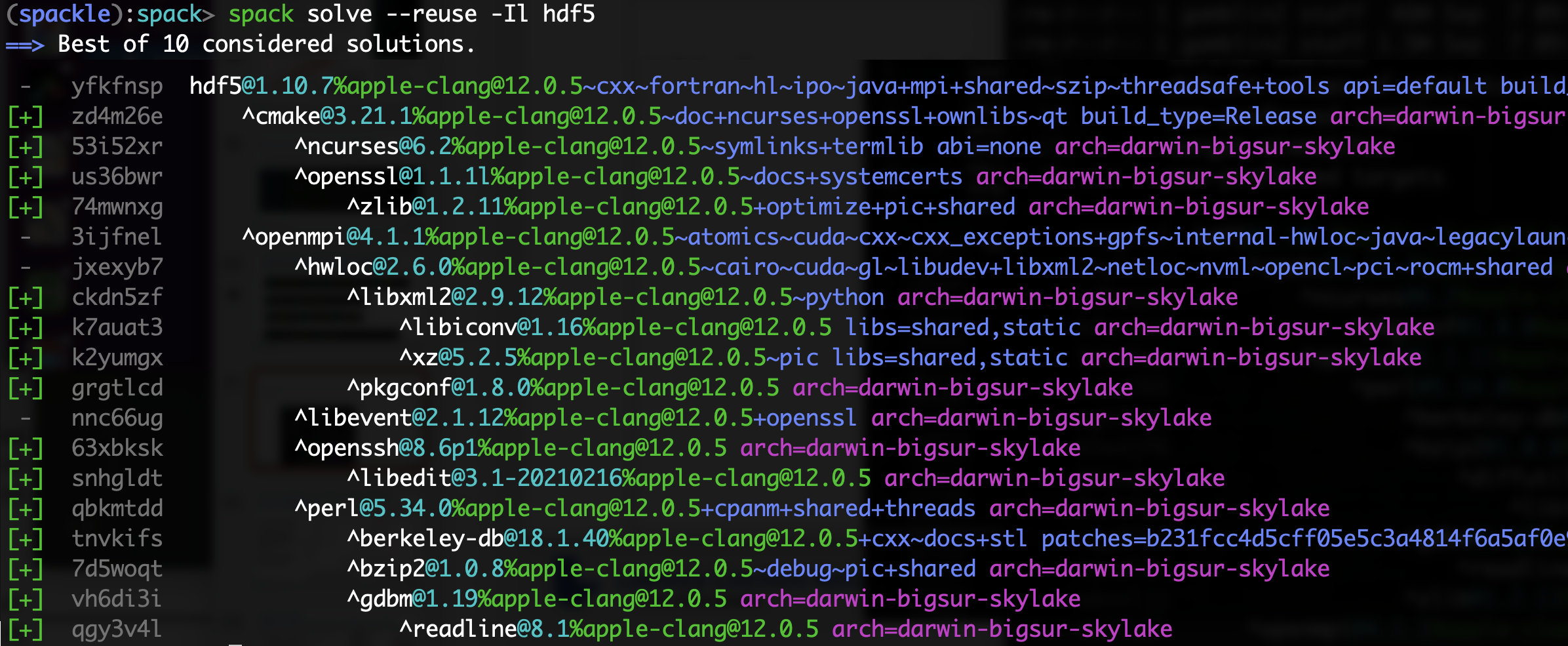
(b)

Figure 6: Concretization with and without reuse optimization.

VII Performance Results

The clingo solver performance given a logic program depends on a number of factors. First, the number of facts in a specific concretization. Second, the configuration and various optimization parameters passed to the solver.

The solving process consists of four stages: setup, load, ground, and solve. The first two are preliminary phases and the other two perform the solve. Specifically, the setup phase generates the facts for the given spec, whereas the load phase loads the main logic program (i.e., the rules of the software model) as a resource into the solver. The grounding phase comes first. Once we have a grounded program, we can run the last phase: the full solve in clingo. We instrumented the solver to measure each phase.

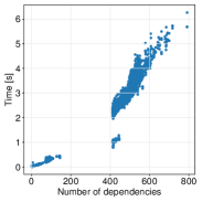
(a)

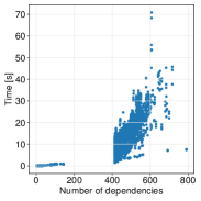
(b)

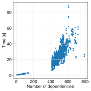
(c)

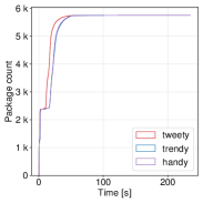
(d)

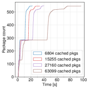
(e)

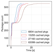
(f)

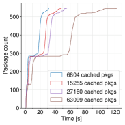
(g)

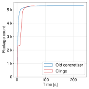
(h)

Figure 7: Performance figures of solving times across all packages on Quartz.

VII-A System Setup

All performance runs were executed on a single node each of the Quartz and Lassen supercomputers at at Lawrence Livermore National Laboratory (LLNL) [43]. Quartz is an Intel-based 3.3 PF machine, where each node comprises two Intel Xeon E5-2695 v4 (Haswell) processors and 128GB of memory. The Lassen machine is a smaller variant of Sierra, a 125 PF capability supercomputer at LLNL. Each node on Lassen has two IBM Power9 little-endian processors and four NVIDIA Tesla V100 (Volta) GPUs. There are 256GB of memory on each node. No hardware accelerators were used in any of our testing. Experiments ran with NFSv3.

VII-B Solve timings for all packages

In this section we examine the solving times for all the packages. First, we focus on the relation between the solving times and the number of dependencies for each package.

For number of dependencies, we measured the number of possible dependencies added to the solve, rather than the total dependencies in the result, because it is a closer measure of the necessary work for the solver. This leads to natural clustering in the number of dependencies, as many simple dependencies lead to large numbers of potential dependencies that dwarf other differences between specs.

Figures 7a, 7b, and  7c show the grounding, solve, and full solving (i.e., involving all the stages) times for all the packages on Quartz. The results on Lassen are comparable to Quartz and are omitted to save space. Load times, as one would expect, were not affected by the number of packages. Also, the setup times are the same order of magnitude as ground times and do not depend on clingo’s performance so they were omitted in favor of showing times that are directly dependent on clingo. We used the clingo’s tweety configuration and unsatisfiable-core-guided optimization strategy (usc,one) for running the solving process. Further below we explore the differences in solving times between these different strategies.

We can see from the figures that the time increases as the number of possible dependencies increases. This is because more dependencies lead to more facts and a bigger logic program overall. We measure possible dependencies rather than actual dependencies because possible dependencies better measure the size of the problem space. In particular, when many packages can provide a virtual dependency like the Message Passing Interface (MPI), much of the potential solve space is not present in the final result when a single MPI implementation is chosen.

Figure 7c also shows that there are two major clusters in the execution times. The clusters are separated by a gap in the possible dependencies. One cluster contains packages with less than 200 possible dependencies, whereas, the other major cluster contains packages with more than 400 possible dependencies. This natural clustering occurs because some low-level dependencies have options that can trigger huge potential dependency trees, and the gap is between packages that can include those dependencies and those that cannot. For example, any package that can depend on MPI in any possible configuration of it and its dependencies involves at least 452 possible dependencies. Since many unusual but technically valid package configurations can create circular dependencies between MPI and build tools (e.g. mpilander provides MPI and mpilander -> cmake -> qt -> valgrind -> mpi), in practice a gap forms between the packages that (mostly) all can depend on MPI, and those that cannot. While the solver excludes the configurations that actually produce circular dependencies, these cycles expand the solution space of the solver and therefore affect performance.

Besides dependencies another set of factors that influences the execution times are clingo parameters. Specifically, clingo defines six configuration presets: frumpy, jumpy, tweety, trendy, crafty, and handy. Each preset sets numerous low level parameters that control different aspects of the solver. In our performance study, we specifically focus on three configurations: tweety – geared towards typical ASP programs, trendy – geared towards industrial problems, and handy – geared towards large problems.

Figure 7d shows the cumulative distribution of full solve times tweety, trendy, and handy configurations on Quartz. The results on Lassen are comparable to Quartz and are omitted to save space. The vast majority of packages are fully solved in under 25 seconds, and most are solved in less than 10 seconds. We also saw (figure omitted) that there is no difference in ground times between the different configurations. This suggests that most low level parameters that are tweaked by each configuration control the actual solving phase. The figures clearly indicate that tweety performs better than the other configurations we benchmarked. We therefore chose it as our default configuration for concretization.

Figure 7h shows the the cumulative distribution of the old concretizer times and clingo total solve times (under the tweety configuration) on Quartz. From it, we see that about 2.2K packages belong to the cluster with less than 200 dependencies in Figure 7c, which means that the dependency trees of these packages are smaller. This leads to shorter ground and solve times and that makes clingo’s times correspond to old concretizer times for these packages. The packages in the other cluster have potentially huge dependency trees that increase the total solving times and that is reflected in the deviation of clingo’s times in Figure 7h from the old concretizer times.

VII-C Solve timings for all packages with reuse

In this subsection, we examine the performance of the solver with the reuse flag switched on. As described in Section VI, reusing packages in a buildcache increases the number of facts proportionally to the number of cached packages.

We specifically focus on the packages in the ECP Extreme-scale Scientific Software Stack (E4S) project [14]. It is a community effort to provide open source software packages for developing, deploying, and running scientific applications on HPC platforms. There are just under 600 packages in E4S, but the buildcache of the project targets different architectures, operating systems, and compilers, thereby totaling over 60K pre-compiled packages (hash signatures). We divided the buildcache into 4 groups: full buildcache (63099 packages), buildcache restricted to the ppc64le architecture (27160 packages), buildcache restricted to the rhel7 OS (15255 packages), and buildcache restricted to both ppc64le architecture and the rhel7 OS (6804 packages). Benchmarking across an increasing size of the buildcache provides us with a better understanding of the impact of reuse optimization.

Figures 7e, 7f, and 7g show the cumulative distribution of the solve times of the E4S packages with increasing buildcache on Quartz. The results on Lassen are comparable to Quartz and are omitted to save space. Setup times are higher than solve times, even for smaller buildcaches. This happens because when we reuse packages we need to load the database of existing packages. This is currently time consuming because it requires us to read and compare many spec objects in Python. There a jump in the solve times for the largest buildcache, but most solves take less than 10 seconds. The fact that the runtime is dominated by serial setup time is good news; setup time is easily optimized away through caching and optimizing Python code, while solve time is not. The E4S buildcache, with nearly 64,000 packages, is much larger than most package repositories, and we expect that our approach will scale to much larger buildcaches if we can optimize the Python runtime. Multi-shot solver techniques may offer additional solver performance, as we can divide and conquer for a slightly less optimal final result.

VIII Conclusions

The complexity of software dependencies and optimization needs in HPC creates a particular challenge for package management in the HPC space. Ad-hoc techniques for dependency resolution have proven to require substantial investment of programmer hours to manage even a small subset of the possible space of HPC software configurations.

In this paper we introduced a new dependency resolution method for Spack, an HPC package manager. This new dependency resolution method uses Answer Set Programming to model Spack’s DSL, compatibility semantics, and optimization rules in a maintainable, declarative syntax. It has allowed us to implement new functionality for Spack, such as targeted reuse of installations and binary packages, that was simply infeasible with previous methods reliant on a greedy fixed-point algorithm. We showed that the performance of the new concretizer is competitive with the previous algorithm, and that performance of the reuse capability is scalable.

References

- Hoste et al. [2012] K. Hoste, J. Timmerman, A. Georges, and S. D. Weirdt, “Easybuild: Building software with ease,” in 2012 SC Companion: High Performance Computing, Networking Storage and Analysis, 2012, pp. 572–582.
- Gamblin et al. [2015] T. Gamblin, M. P. LeGendre, M. R. Collette, G. L. Lee, A. Moody, B. R. de Supinski, and W. S. Futral, “The Spack Package Manager: Bringing order to HPC software chaos,” in Supercomputing 2015 (SC’15), Austin, Texas, November 15-20 2015, LLNL-CONF-669890.
- Dubois et al. [2003] P. F. Dubois, T. Epperly, and G. Kumfert, “Why johnny can’t build [portable scientific software],” Computing in Science Engineering, vol. 5, no. 5, pp. 83–88, 2003.
- Hochstein and Jiao [2011] L. Hochstein and Y. Jiao, “The cost of the build tax in scientific software,” International Symposium on Empirical Software Engineering and Measurement, pp. 384–387, September 2011.
- Falgout et al. [2006] R. Falgout, J. Jones, and U. Yang, “The design and implementation of hypre, a library of parallel high performance preconditioners,” in Numerical Solution of Partial Differential Equations on Parallel Computers, A. Bruaset and A. Tveito, Eds. Springer-Verlag, 2006, vol. 51, pp. 267–294.
- Anderson et al. [2021] R. Anderson, J. Andrej, A. Barker, J. Bramwell, J.-S. Camier, J. Cerveny, V. Dobrev, Y. Dudouit, A. Fisher, T. Kolev, W. Pazner, M. Stowell, V. Tomov, I. Akkerman, J. Dahm, D. Medina, and S. Zampini, “MFEM: A Modular Finite Element Methods Library,” Computers & Mathematics with Applications, vol. 81, pp. 42–74, January 2021.
- [7] “Portable, Extensible Toolkit for Scientific Computation (PETSc),” http://www.mcs.anl.gov/petsc.
- Heroux et al. [2005] M. A. Heroux, R. A. Bartlett, V. E. Howle, R. J. Hoekstra, J. J. Hu, T. G. Kolda, R. B. Lehoucq, K. R. Long, R. P. Pawlowski, E. T. Phipps, A. G. Salinger, H. K. Thornquist, R. S. Tuminaro, J. M. Willenbring, A. Williams, and K. S. Stanley, “An overview of the Trilinos project,” ACM Trans. Math. Softw., vol. 31, no. 3, pp. 397–423, 2005.
- Hornung and Keasler [2014] R. D. Hornung and J. A. Keasler, “The RAJA Portability Layer: Overview and Status,” Lawrence Livermore National Laboratory, Tech. Rep. LLNL-TR-661403, Sep. 2014.
- Edwards et al. [2014] H. C. Edwards, C. R. Trott, and D. Sunderland, “Kokkos: Enabling manycore performance portability through polymorphic memory access patterns,” Journal of Parallel and Distributed Computing, vol. 74, pp. 3202–3216, Dec. 2014. [Online]. Available: http://www.sciencedirect.com/science/article/pii/S0743731514001257
- Bicking [2011] I. Bicking, “pip: Package Install tool for Python,” April 2011, https://github.com/pypa/pip.
- Schlueter [2009] I. Z. Schlueter, “NPM,” Online, September 2009, https://github.com/npm/npm.
- car [2014] “Cargo: The Rust package manager,” Online, March 2014, https://github.com/rust-lang/cargo.
- [14] “The Extreme-scale Scientific Software Stack (E4S),” https://e4s-project.github.io/.
- Dolstra and Löh [2008] E. Dolstra and A. Löh, “NixOS: A Purely Functional Linux Distribution,” in Proceedings of the 13th ACM SIGPLAN International Conference on Functional Programming, ser. ICFP ’08. New York, NY, USA: ACM, 2008, pp. 367–378.
- Dolstra et al. [2004] E. Dolstra, M. de Jonge, and E. Visser, “Nix: A Safe and Policy-Free System for Software Deployment,” in Proceedings of the 18th Large Installation System Administration Conference (LISA XVIII), ser. LISA ’04. Berkeley, CA, USA: USENIX Association, 2004, pp. 79–92.
- Di Cosmo [2005] R. Di Cosmo, “EDOS deliverable WP2-D2.1: Report on Formal Management of Software Dependencies,” INRIA, Tech. Rep., May 15 2005, hal-00697463.
- Cox [2016] R. Cox, “Version SAT: Dependency hell is NP-complete. But maybe we can climb out.” Online, December 13 2016, https://research.swtch.com/version-sat.
- Abate et al. [2020] P. Abate, R. Di Cosmo, G. Gousios, and S. Zacchiroli, “Dependency solving is still hard, but we are getting better at it,” in 2020 IEEE 27th International Conference on Software Analysis, Evolution and Reengineering (SANER). IEEE, 2020, pp. 547–551.
- Gebser et al. [2012] M. Gebser, R. Kaminski, B. Kaufmann, and T. Schaub, “Answer set solving in practice,” Synthesis lectures on artificial intelligence and machine learning, vol. 6, no. 3, pp. 1–238, 2012.
- Marek et al. [2011] V. W. Marek, I. Niemelä, and M. Truszczynski, “Origins of answer-set programming - some background and two personal accounts,” CoRR, vol. abs/1108.3281, 2011. [Online]. Available: http://arxiv.org/abs/1108.3281
- Van Der Hoek et al. [1997] A. Van Der Hoek, R. S. Hall, D. Heimbigner, and A. L. Wolf, “Software release management,” ACM SIGSOFT Software Engineering Notes, vol. 22, no. 6, pp. 159–175, 1997.
- Ewing and Troan [1995] M. Ewing and E. Troan, “RPM Timeline,” Online, 1995, https://rpm.org/timeline.html.
- Gunthorpe [1998] J. Gunthorpe, “APT User’s Guide,” Online, 1998, https://www.debian.org/doc/manuals/apt-guide/.
- Foster-Johnson [2003] E. Foster-Johnson, “Red Hat RPM Guide,” 2003.
- Silva [2001] G. N. Silva, “APT Howto,” Debian, Tech. Rep., 2001, http://www. debian. org/doc/manuals/apt-howto.
- [27] T. F. Project, “Yellowdog Updater, Modified (YUM),” http://yum.baseurl.org.
- Mancinelli et al. [2006] F. Mancinelli, J. Boender, R. di Cosmo, J. Vouillon, B. Durak, X. Leroy, and R. Treinen, “Managing the complexity of large free and open source package-based software distributions,” in 21st IEEE/ACM International Conference on Automated Software Engineering (ASE’06), 2006, pp. 199–208.
- Abate et al. [2012] P. Abate, R. Di Cosmo, R. Treinen, and S. Zacchiroli, “Dependency solving: a separate concern in component evolution management,” Journal of Systems and Software, vol. 85, no. 10, pp. 2228–2240, 2012.
- Abate et al. [2013] P. Abate, R. Di Cosmo, R. Treinen, and S. Zacchiroli, “A modular package manager architecture,” Information and Software Technology, vol. 55, no. 2, pp. 459 – 474, 2013, special Section: Component-Based Software Engineering (CBSE), 2011. [Online]. Available: http://www.sciencedirect.com/science/article/pii/S0950584912001851
- Tucker et al. [2007] C. Tucker, D. Shuffelton, R. Jhala, and S. Lerner, “Opium: Optimal package install/uninstall manager,” in Proceedings of the 29th International Conference on Software Engineering, ser. ICSE ’07. USA: IEEE Computer Society, 2007, pp. 178–188.
- Michel and Rueher [2010] C. Michel and M. Rueher, “Handling software upgradeability problems with MILP solvers,” in Proceedings First International Workshop on Logics for Component Configuration, LoCoCo 2010, Edinburgh, UK, 10th July 2010, ser. EPTCS, I. Lynce and R. Treinen, Eds., vol. 29, 2010, pp. 1–10. [Online]. Available: https://doi.org/10.4204/EPTCS.29.1
- Argelich et al. [2010] J. Argelich, D. Le Berre, I. Lynce, J. P. M. Silva, and P. Rapicault, “Solving linux upgradeability problems using boolean optimization,” in Proceedings First International Workshop on Logics for Component Configuration, LoCoCo 2010, Edinburgh, UK, 10th July 2010, ser. EPTCS, I. Lynce and R. Treinen, Eds., vol. 29, 2010, pp. 11–22. [Online]. Available: https://doi.org/10.4204/EPTCS.29.2
- Gebser et al. [2011a] M. Gebser, R. Kaminski, and T. Schaub, “aspcud: A linux package configuration tool based on answer set programming,” Electronic Proceedings in Theoretical Computer Science, vol. 65, pp. 12–25, Aug 2011.
- Weizenbaum [2018] N. Weizenbaum, “PubGrub: Next-Generation Version Solving,” https://medium.com/@nex3/pubgrub-2fb6470504f, April 2 2018.
- Python Software Foundation [2020] Python Software Foundation, “New pip resolver to roll out this year,” Online, March 23 2020, https://pyfound.blogspot.com/2020/03/new-pip-resolver-to-roll-out-this-year.html.
- Courtès and Wurmus [2015] L. Courtès and R. Wurmus, “Reproducible and User-Controlled Software Environments in HPC with Guix,” in 2nd International Workshop on Reproducibility in Parallel Computing (RepPar), Vienne, Austria, Aug. 2015. [Online]. Available: https://hal.inria.fr/hal-01161771
- Baral [2003] C. Baral, Declarative programming in AnsProlog*: introduction and preliminaries. Cambridge University Press, 2003, pp. 1–45.
- Moskewicz et al. [2001] M. W. Moskewicz, C. F. Madigan, Y. Zhao, L. Zhang, and S. Malik, “Chaff: Engineering an efficient sat solver,” in Proceedings of the 38th annual Design Automation Conference, 2001, pp. 530–535.
- Gebser et al. [2011b] M. Gebser, B. Kaufmann, R. Kaminski, M. Ostrowski, T. Schaub, and M. Schneider, “Potassco: The potsdam answer set solving collection,” AI Communications, vol. 24, no. 2, pp. 107–124, 2011.
- Davis and Putnam [1960] M. Davis and H. Putnam, “A computing procedure for quantification theory,” J. ACM, vol. 7, no. 3, pp. 201–215, jul 1960. [Online]. Available: https://doi.org/10.1145/321033.321034
- Davis et al. [1962] M. Davis, G. Logemann, and D. Loveland, “A machine program for theorem-proving,” Commun. ACM, vol. 5, no. 7, pp. 394–397, jul 1962. [Online]. Available: https://doi.org/10.1145/368273.368557
- [43] “Lawrence Livermore National Laboratory HPC Compute Platforms,” https://hpc.llnl.gov/hardware/compute-platforms.