Distributed Estimation and Inference for Semi-parametric Binary Response Models

Abstract

The development of modern technology has enabled data collection of unprecedented size, which poses new challenges to many statistical estimation and inference problems. This paper studies the maximum score estimator of a semi-parametric binary choice model under a distributed computing environment without pre-specifying the noise distribution. An intuitive divide-and-conquer estimator is computationally expensive and restricted by a non-regular constraint on the number of machines, due to the highly non-smooth nature of the objective function. We propose (1) a one-shot divide-and-conquer estimator after smoothing the objective to relax the constraint, and (2) a multi-round estimator to completely remove the constraint via iterative smoothing. We specify an adaptive choice of kernel smoother with a sequentially shrinking bandwidth to achieve the superlinear improvement of the optimization error over the multiple iterations. The improved statistical accuracy per iteration is derived, and a quadratic convergence up to the optimal statistical error rate is established. We further provide two generalizations to handle the heterogeneity of datasets with covariate shift and high-dimensional problems where the parameter of interest is sparse.

1 Introduction

In many statistical applications, the phenomena that practitioners would like to explain are dichotomous: the outcome/response can take only two values. This model, usually referred to as binary response model, is central to a wide range of fields such as applied econometrics, pharmaceutical studies, clinical diagnostics, and political sciences. The most commonly used parametric approaches, notably logit and probit models, assume that the functional form of the model, typically the distribution of the response variable conditional on the explanatory variables, is known. Nonetheless, there is usually little justification for assuming that the functional form of conditional probability is known in practice. Once the functional form is misspecified, the estimate of the underlying parameter of interest and the corresponding inference results can be highly misleading (see White, 1982; Horowitz, 1993; Horowitz and Spokoiny, 2001; Greene, 2009 for illustration). To balance between the potential model misspecification in parametric models and the curse of dimensionality in non-parametric models, practitioners may assume that the threshold, instead of the conditional probability, can be approximated by some pre-specified function.

In this paper, we consider the semi-parametric binary response models of the following form:

$$Y=\mathrm{sign}\left(Y^{*}\right)\in\{-1,+1\},\quad Y^{*}=X+\bm{Z}^{\top}\bm{\beta}^{*}+\epsilon,\quad\bm{\beta}^{*}\in\mathbb{R}^{p},$$ (1)

where $Y$ is the binary response variable, $X$ and $\bm{Z}$ are covariates, and $\epsilon$ denotes a random noise that is not required to be independent of $\bm{Z}$. Assume that $\{\left(y_{i},x_{i},\bm{z}_{i},\epsilon_{i}\right)\}_{i=1,2,\dots,n}$ are i.i.d. copies of $\left(Y,X,\bm{Z},\epsilon\right)$. Our goal is to estimate $\bm{\beta}^{*}$ given $\{\left(y_{i},x_{i},\bm{z}_{i}\right)\}_{i=1,2,\dots,n}$. If the distribution of the noise $\epsilon$ is pre-specified, the model becomes a traditional parametric model such as the probit model (for normal noise) and logit model (for logistic noise). However, as misspecification of the noise distribution may cause poor estimation, practitioners prefer to use a semi-parametric model to estimate $\bm{\beta}^{*}$. Manski (1975) proposed the Maximum Score Estimator (MSE),

$$\widehat{\bm{\beta}}_{\rm{MSE}}=\operatorname*{\arg\!\max}_{\bm{\beta}\in\mathbb{R}^{p}}\frac{1}{n}\sum_{i=1}^{n}\left[\mathbb{I}\left(y_{i}=1,x_{i}+\bm{z}_{i}^{\top}\bm{\beta}\geq 0\right)+\mathbb{I}\left(y_{i}=-1,x_{i}+\bm{z}_{i}^{\top}\bm{\beta}<0\right)\right],$$ (2)

where $\mathbb{I}(\cdot)$ denotes the indicator function. Manski refers to the objective function in (2) as a score function, and the estimator $\widehat{\bm{\beta}}_{\rm{MSE}}$ is obtained via maximizing the score function. The statistical properties of MSE have been well-studied in the literature (Chamberlain, 1986; Kim and Pollard, 1990). Nonetheless, the existing literature rarely examines the practical feasibility to achieve the estimator in a large dataset, even though it is essential to make use of the estimator in real-world applications. Despite a macroscopical intuition underneath the optimization problem (2), the objective function is hard to optimize due to non-convexity and non-smoothness, especially when the sample size is large.

Indeed, the rapid development of modern technology has enabled data collection of unprecedented size. Such a large amount of data are usually generated and subsequently stored in a decentralized fashion. Due to the concerns of data privacy, data security, ownership, transmission cost, and others, the decentralized data may not be pooled (Zhou et al., 2018). In distributed settings, classical statistical results, which are developed under the assumption that the datasets across different local machines can be pooled together, are no longer applicable. Therefore, many estimation and inference methods need to be re-investigated.

In a distributed setting, a common estimation strategy is the divide-and-conquer (DC) algorithm, which estimates a local estimator on each local machine and then aggregates the local estimators to obtain the final estimator (please refer to Section 1.1 below for a detailed discussion of existing literature). Combining the idea of DC with the maximum score estimator (MSE) intuitively leads to a divide-and-conquer MSE (Avg-MSE) approach, where one can solve an MSE on each local machine and then aggregate the obtained solutions by an averaging operation. We use $n$ to denote the total sample size and assume that the data is stored on $L$ machines where each machine has $m=n/L$ data points. Shi et al. (2018) studied the (Avg-MSE) approach and obtained a convergence rate $O(L^{-\frac{1}{2}}m^{-\frac{1}{3}})$ under a restrictive constraint on the number of local machines: $L=o(m^{\frac{1}{6}})$, ignoring the logarithm term. Therefore, given $m$, the established analysis is only valid as $L=n/m$ increases to $O(m^{\frac{1}{6}})$, after which the estimator will not improve anymore. In other words, the best convergence rate that (Avg-MSE) can achieve is limited to $O\big{(}(m^{\frac{1}{6}})^{-\frac{1}{2}}m^{-\frac{1}{3}}\big{)}=O(m^{-\frac{5}{12}})$, regardless of how large the total sample size $n$ is. Besides the aforementioned limitation on slow convergence rate and the constraint of $L$, the limiting distribution of MSE cannot be given in an explicit form (Kim and Pollard, 1990), and hence it can be hard in practice to apply it for inference. Additionally, an exact solver of MSE requires solving a mixed integer programming, which is computationally heavily demanding when the dimension $p$ is large.

In order to improve the convergence rate and relax the restriction on the number of machines, we first consider a natural alternative, an averaged smoothed maximum score estimator (Avg-SMSE) which optimizes a smoothed version of the MSE objective (Horowitz, 1992) on each local machine and then aggregates the obtained estimators by averaging. In contrast to (Avg-MSE), (Avg-SMSE) achieves a convergence rate $O\big{(}n^{-\frac{\alpha}{2\alpha+1}}\big{)}$ under a constraint $L=o\big{(}m^{\frac{2}{3}\left(\alpha-1\right)}\big{)}$, ignoring the logarithm term, where $\alpha$ is the smoothness parameter of the kernel function used to smooth the objective function. This implies that given $m$, the best achievable convergence rate is $O(m^{-\frac{\alpha}{3}})$, regardless of how large $n$ is. When $\alpha\geq 2$, (Avg-SMSE) achieves a convergence rate of at least $O(m^{-\frac{2}{3}})$, faster than that of (Avg-MSE), under a weakened constraint of $L$. The detailed algorithm is described in Section 2.2 and the theoretical analysis of (Avg-SMSE) is presented in Section 3.1. The analysis of (Avg-SMSE) is not trivially adopted from that of (Avg-MSE), since it involves handpicking an optimal bandwidth $h$ to balance the bias and variance.

The analysis reveals a fundamental bottleneck in divide-and-conquer algorithms: the bias-variance trade-off in the mean squared error analysis. In many statistical problems under a non-distributed environment, an asymptotic unbiased estimator is often satisfactory as it enables theorists to establish the asymptotic normality and design statistical inference procedures based on the asymptotic distribution, even though the order of the asymptotic bias depends on the sample size. Nonetheless, in a distributed environment, the biases across multiple local machines cannot be reduced by aggregation. When the number of machines $L$ is large, the bias term of the divide-and-conquer estimator is dominant in the estimation error, which leads to an efficiency loss and limits the improvement of the divide-and-conquer algorithms as the total sample size $n$ increases. In an extreme scenario, as the local sample size $m$ stays fixed and $L$ increases, the convergence rate of the divide-and-conquer algorithms does not improve. Unfortunately, this scenario is indeed more practically realistic as each local machine (a database) has its storage limit but the number of machines may always be increasing.

To feature the scenario that $L$ exceeds $m^{\frac{2}{3}(\alpha-1)}$, this paper further proposes a new approach called multi-round Smoothed Maximum Score Estimator (mSMSE) in Section 2.3, which successively refines the estimator with multiple iterations. In iteration $t$, the algorithm implements a Newton step to optimize the smoothed objective function governed by a smoothing parameter $h_{t}$. Over the multiple rounds, the algorithm iteratively smooths the score function (2) by a diminishing sequence $\{h_{t}\}$. The decay rate of $\{h_{t}\}$ is carefully designed by examining the rate improvement in each iteration of the algorithm, details of which are provided in Section 3.2. Under this iterative smoothing scheme, the proposed (mSMSE) converges to the optimal statistical rate $O(n^{-\frac{\alpha}{2\alpha+1}})$ in $O(\log\log n)$ iterations and is scalable in dimension and computationally efficient. More specifically, the algorithm performs a quadratic (superlinear) convergence across iterations until it reaches the optimal accuracy. We thereafter establish the asymptotic normality of (mSMSE) in Theorem 3.4, followed by a bias-correction procedure to construct the confidence interval of (mSMSE) from samples in Corollary 3.5 for the purpose of distributed inference.

Lastly, we consider two important extensions of the proposed methods. First, an important question in distributed environments is the heterogeneity of datasets on different local machines. In Section 4.1, we consider heterogeneous datasets with a shared parameter of interest $\bm{\beta}^{\star}$ and different distributions of covariates $(X,\bm{Z})$ across the machines. We show that (mSMSE) performs better than (Avg-SMSE) with a weaker condition. While handling heterogeneous data, the performance of the divide-and-conquer algorithm relies on the smallest sample size among the local machines, while the (mSMSE) method does not rely on such conditions.

We further consider a high-dimension extension in Section 4.2 where the parameter of interest $\bm{\beta}^{*}\in\mathbb{R}^{p}$ is a sparse vector with $s$ non-zero elements and $s<n<p$. We modify (mSMSE) to adapt the idea of the Dantzig Selector (Candes and Tao, 2007) to reach the convergence rate $\sqrt{s}(\log p/n)^{\frac{\alpha}{2\alpha+1}}$ in a distributed environment, which is very close to the minimax optimal rate $(s\log p/n)^{\frac{\alpha}{2\alpha+1}}$ for the linear binary response model established by Feng et al. (2022) in a non-distributed environment. Compared to the low-dimensional settings above, the algorithm in this setting reduces the per-iteration communication cost to $p\times 1$ vectors.

We emphasize the technical challenges below and summarize the methodology contribution and theoretical advances compared to the existing literature.

• We propose two algorithms for distributed estimation and inference based on (1) a divide-and-conquer estimator (Avg-SMSE) that improves the convergence rate and relaxes the constraint on $L$ of (Avg-MSE) in Shi et al. (2018), and (2) a multi-round estimator (mSMSE) that sequentially smooths the objective function and refines the estimator. The second algorithm ensures a fast (quadratic) convergence over iterations toward optimal statistical accuracy and can be applied even to non-distributed settings as an efficient computational algorithm to solve MSE on the pooled dataset. We further show that (mSMSE) achieves the same statistical efficiency uniformly over a class of models in a neighborhood of the given model.

• The non-smoothness in the objective function is the major technical challenge. Existing algorithms for distributed estimation rarely handle non-smooth objectives, with a few exceptions that either provide statistical results without algorithmic guarantee or heavily rely on subgradient-based algorithms to solve the convex objective. However, the subgradient of (2) is almost everywhere zero. The proposed (mSMSE) handles this challenge by carefully identifying a smoothing objective to approximate (2), which varies over the iterations. The proposed procedure shares the spirit of the Newton-type multi-round algorithms established for smooth objectives in Jordan et al. (2019) and Fan et al. (2021). Nonetheless, the proposed (mSMSE) is not an application of the algorithms therein, but instead maximizes different smoothed objectives over multiple iterations. Indeed, to achieve the optimal statistical rate, the optimal bandwidth needs to be as small as $O(n^{-\frac{1}{2\alpha+1}})$. Nevertheless, such a choice of bandwidth is invalid in the earlier stage of the proposed procedure, and it is therefore critical to specify an iteratively decreasing sequence of bandwidths properly.

• Another technical challenge appears in establishing the multi-round refinements. In each iteration, the initial estimator is the output of the last iteration which has already utilized the complete sample and is therefore data-dependent. Therefore, it requires establishing a quantification of the improvement in each iteration uniformly for any initial estimator in a neighborhood of the truth. In addition, as the algorithm proceeds, the smoothed surrogate approaches better to the discontinuous objective (2), whereas the Lipschitz condition of its gradient diverges exponentially, bringing challenges to establishing concentration inequalities.

• Lastly, in high-dimensional settings, neither the non-smooth objective nor the smoothed objective is guaranteed to be convex, which causes difficulty in applying the $\ell_{1}$-regularization methods. Instead, we adopt the Dantzig estimator in each iteration to make the optimization problem feasible while encouraging the sparse structure.

The remainder of the paper is organized as follows: In Section 1.1, we review the related literature on distributed estimation and inference. Section 2 describes the methodology of the proposed (Avg-SMSE) and (mSMSE) procedures. Sections 3.1–3.2 present the theoretical results for the two estimators, respectively. Section 3.3 uses the asymptotic results to facilitate distributed inference. In Section 4.1, we discuss the effect of heterogeneity on distributed inference. In Section 4.2, we modify (mSMSE) to apply to high-dimensional semi-parametric binary response models. Numerical experiments in Section 5 lend empirical support to our theory, followed by conclusions and future directions in Section 6. Further discussions and additional theoretical and experimental results including all technical proofs are relegated to Appendix.

1.1 Related Works

For distributed estimation and large-scale data analysis, the divide-and-conquer (DC) strategy has been recently adopted in many statistical estimation problems (see, e.g., Zhang et al., 2012; Li et al., 2013; Chen and Xie, 2014; Zhang et al., 2015; Zhao et al., 2016; Lee et al., 2017; Battey et al., 2018; Shi et al., 2018; Banerjee et al., 2019; Huang and Huo, 2019; Volgushev et al., 2019; Fan et al., 2019). The DC strategy is utilized to handle massive data when the practitioner observes a large-scale centralized dataset, partitions it into subsamples, performs an estimation on each subsample, and finally aggregates the subsample-level estimates to generate a (global) estimator. The divide-and-conquer principle also fits into the scenarios where datasets are collected and stored originally in different locations (local machines), such as sensor networks, and cannot be centralized due to high communication costs or privacy concerns. A standard DC approach computes a local estimator (or local statistics) on each local machine and then transports them to the central machine in order to obtain a global estimator by appropriate aggregation. Recently, Shi et al. (2018) and Banerjee et al. (2019) studied the divide-and-conquer principle in non-standard problems such as isotonic regression and cube-root M-estimation. They showed that the DC strategy improves the statistical rate of the cubic-rate estimator, while the aggregated estimators often entail the super-efficiency phenomenon, a circumvention of which is proposed by Banerjee and Durot (2019) via synthesizing certain summary statistics on local machines instead of aggregating the local estimators.

DC approaches often require a restriction that the number of machines (subgroups) does not increase very fast compared to the smallest local subsample size, such as to retain the optimal statistical efficiency of the DC estimators. Such a restriction can be stringent in many decentralized systems with strong privacy and security concerns. The restriction deteriorates in many non-standard problems, due to the nonsmoothness of the objective functions. In these scenarios, Shamir et al. (2014), Wang et al. (2017) and Jordan et al. (2019) proposed multi-round procedures for refinement, followed by Fan et al. (2021), Chen et al. (2021), Tu et al. (2021), Luo et al. (2022), and others. These frameworks typically use outputs of the preceding iteration as input for the succeeding iterations. After a number of rounds, the estimator is refined to achieve the optimal statistical rate. Such procedures, typically performed with continuous optimization algorithms, are generally inapplicable to non-smooth problems due to their requirement that the loss function needs to be sufficiently smooth, although a non-smooth regularization term is permitted.

The understanding of the multi-round improvement under the non-smooth scenarios is still in many ways nascent, and existing analyses mostly depend on the specific statistical model. Chen et al. (2019), Wang et al. (2019), Chen et al. (2021), and Tan et al. (2021) proposed remedies for specific continuous objective functions that violate second-order differentiability, mainly featuring quantile regression and linear support vector machines. Other estimators obtained by minimizing non-smooth objectives must be analyzed in a case-by-case scenario, as a non-smooth loss usually leads to a slow rate of statistical convergence as well as deficiencies in algorithmic convergence. In this paper, we spotlight the semi-parametric binary response model whose corresponding loss function is non-convex and not continuous, both violating the assumptions in the above literature.

For distributed inference, existing works, for example, Jordan et al. (2019), Chen et al. (2021), and others, established asymptotic normality for their distributed estimators and yielded distributed approaches to construct confidence regions using the sandwich-type covariance matrices. In addition to the above, Yu et al. (2020, 2022) proposed distributed bootstrap methods for simultaneous inference in generalized linear models that allow a flexible number of local machines. Wang and Zhu (2022) proposed a bootstrap-and-refitting procedure that improved the one-shot performance of distributed bootstrap via refitting.

1.2 Notations

For any vector $\bm{v}=\left(v_{1},..,v_{p}\right)\in\mathbb{R}^{p}$, we denote the $\ell_{q}$-norm by $\|\bm{v}\|_{q}:=\left(\sum_{k=1}^{p}|v_{k}|^{q}\right)^{1/q}$ and the $\ell_{\infty}$-norm by $\|\bm{v}\|_{\infty}:=\max_{k}|v_{k}|$. Denote by $\bm{v}_{S}=\left(v_{i_{1}},v_{i_{2}},...,v_{i_{s}}\right)^{\top}$ for any given $S=\{i_{1},i_{2},...,i_{s}\}\subset\{1,2,...,p\}$. For any matrix $A=\left(a_{ij}\right)$, we define $\|A\|_{1}=\max_{j}\left(\sum_{i}|a_{ij}|\right)$, $\|A\|_{2}=\max_{\|\bm{v}\|_{2}=1}\|A\bm{v}\|_{2}$, $\|A\|_{\infty}=\max_{i}\left(\sum_{j}|a_{ij}|\right)$, and $\|A\|_{\max}:=\max_{i,j}|a_{ij}|$. Also, for a sequence of random variables $X_{n}$ and a sequence of real numbers $a_{n}$, we let $X_{n}=O_{\mathbb{P}}(a_{n})$ denote that $\left\{X_{n}/a_{n}\right\}$ is bounded in probability and $X_{n}=o_{\mathbb{P}}(a_{n})$ denote that $\left\{X_{n}/a_{n}\right\}$ converges to zero in probability. For any positive sequences $\{a_{n}\}$ and $\{b_{n}\}$, we write $a_{n}\lesssim b_{n}$ if $a_{n}=O(b_{n})$, and $a_{n}\asymp b_{n}$ if $a_{n}\lesssim b_{n}$ and $b_{n}\lesssim a_{n}$.

2 Methodology

2.1 Preliminaries

To estimate $\bm{\beta}^{*}$ in Model (1), Manski (1975) proposed the Maximum Score Estimator (MSE) in (2). The objective function that MSE maximizes is the a score function, which counts the number of correct predictions given $\bm{\beta}$. By rewriting

$$\quad\mathbb{I}\left(y_{i}=1,x_{i}+\bm{z}_{i}^{\top}\bm{\beta}\geq 0\right)+\mathbb{I}\left(y_{i}=-1,x_{i}+\bm{z}_{i}^{\top}\bm{\beta}<0\right)=\mathbb{I}\left(y_{i}=-1\right)+y_{i}\mathbb{I}\left(x_{i}+\bm{z}_{i}^{\top}\bm{\beta}\geq 0\right),$$

the maximum score estimator in (2) can be simplified as the following form:

$$\widehat{\bm{\beta}}_{\rm{MSE}}=\operatorname*{\arg\!\min}_{\bm{\beta}\in\mathbb{R}^{p}}F^{*}\left(\bm{\beta}\right):=\operatorname*{\arg\!\min}_{\bm{\beta}\in\mathbb{R}^{p}}\frac{1}{n}\sum_{i=1}^{n}\left(-y_{i}\right)\mathbb{I}\left(x_{i}+\bm{z}_{i}^{\top}\bm{\beta}\geq 0\right).$$ (3)

For the identifiability of $\bm{\beta}^{*}$, as stated in Manski (1985) and Horowitz (1992), we assume the following conditions about the distribution of $X,\bm{Z}$ and $Y$ hold for the entire paper:

1. The median of the noise conditional on $x$ and $\bm{Z}$ is 0, i.e., $\mathrm{median}\left(\epsilon\,|\,X,\bm{Z}\right)=0$.

2. The support of $(X,\bm{Z})$ is not contained in any proper linear subspace of $\mathbb{R}^{p+1}$.

3. For almost every $(X,\bm{Z})$, $0<\mathbb{P}\left(Y=-1\,|\,X,\bm{Z}\right)<1$ .

4. The distribution of $X$ conditional on $\bm{Z}$ has positive density almost everywhere.

See Manski (1985) for the roles that these conditions play in ensuring model identifiability.

The MSE in (2) is known to suffer from a slow rate of convergence due to the discontinuity of the objective function. Specifically, Kim and Pollard (1990) showed that, due to the non-smoothness of the objective function, the MSE is subject to a cubic rate $O\left(n^{-1/3}\right)$, which is slower than the parametric rate $O\left(n^{-1/2}\right)$ of the maximum likelihood estimator. They also established that the limiting distribution of the maximum score estimator cannot be given in an explicit form, and hence it can be hard to apply it in practice for inference.

To overcome the drawbacks of MSE, Horowitz (1992) proposed a Smoothed Maximum Score Estimator (SMSE) by replacing the objective function $F^{*}(\bm{\beta})$ in (3) with a sufficiently smooth function $F_{h}\left(\bm{\beta}\right)$. More specifically, the indicator function $\mathbb{I}\left(\cdot\geq 0\right)$ is approximated by a kernel smoother $H\left(\cdot/h\right)$, where $h$ is the bandwidth, and SMSE is defined as

$$\widehat{\bm{\beta}}_{\rm{SMSE}}:=\operatorname*{\arg\!\min}_{\bm{\beta}\in\mathbb{R}^{p}}F_{h}\left(\bm{\beta}\right)=\operatorname*{\arg\!\min}_{\bm{\beta}\in\mathbb{R}^{p}}\frac{1}{n}\sum_{i=1}^{n}\left(-y_{i}\right)H\Big{(}\frac{x_{i}+\bm{z}_{i}^{\top}\bm{\beta}}{h}\Big{)}.\\$$ (4)

The asymptotic behavior of the smoothed estimator can be analyzed using the classical non-parametric kernel regression theory. The SMSE of $\bm{\beta}^{*}$ is consistent and has a typical non-parametric rate of convergence $n^{-\frac{\alpha}{2\alpha+1}}$, where $\alpha$ is the order of the kernel function (see Assumption 1 for a formal definition). When $\alpha=1$, this convergence rate matches $O\left(n^{-1/3}\right)$ of MSE. When $\alpha\geq 2$, this rate is at least $O\left(n^{-2/5}\right)$, and it can be closer to $O\left(n^{-1/2}\right)$ with a larger $\alpha$. Meanwhile, in contrast to MSE, the limiting distribution of SMSE is in an explicit form, and the parameters in the distribution can be estimated to feature inference applications.

2.2 Divide-and-Conquer SMSE

Under the distributed environment, the data is split into $L$ equally sized subsets (machines) $\{\mathcal{D}_{\ell},\ \ell=1,2\dots,L\}$, where each subset $\mathcal{D}_{\ell}$ has $m=n/L$ data points and the index is denoted by $\mathcal{H}_{\ell}$, i.e., $\mathcal{D}_{\ell}=\{y_{i},x_{i},\bm{z}_{i},i\in\mathcal{H}_{\ell}\}$. A natural solution to a distributed learning task is Divide-and-Conquer via Averaging, which computes a local estimator on each subset and then averages the local estimators over all subsets. Particularly, we define the Averaged Maximum Score Estimator (Avg-MSE) as

$$\widehat{\bm{\beta}}_{\rm{{\tt{(Avg-MSE)}}}}:=\frac{1}{L}\sum^{L}_{\ell=1}\Big{[}\operatorname*{\arg\!\min}_{\bm{\beta}\in\mathbb{R}^{p}}\frac{1}{m}\sum_{i\in\mathcal{H}_{\ell}}\left(-y_{i}\right)\mathbb{I}\left(x_{i}+\bm{z}_{i}^{\top}\bm{\beta}\geq 0\right)\Big{]}.$$ (5)

Analogously, the Averaged Smoothed Maximum Score Estimator (Avg-SMSE) is defined by

$$\widehat{\bm{\beta}}_{\rm{{\tt{(Avg-SMSE)}}}}:=\frac{1}{L}\sum_{\ell=1}^{L}\Big{[}\operatorname*{\arg\!\min}_{\bm{\beta}\in\mathbb{R}^{p}}\frac{1}{m}\sum_{i\in\mathcal{H}_{\ell}}\left(-y_{i}\right)H\Big{(}\frac{x_{i}+\bm{z}_{i}^{\top}\bm{\beta}}{h}\Big{)}\Big{]}.$$ (6)

Shi et al. (2018) showed that the (Avg-MSE) has the convergence rate $O\big{(}L^{-1/2}m^{-1/3}\big{)}$ under the constraint that $L=o\left(m^{1/6}\right)$. In Theorem 3.1, we will show that (Avg-SMSE) achieves the optimal convergence rate $O\big{(}n^{-\frac{\alpha}{2\alpha+1}}\big{)}$ under a constraint that $L=o\big{(}m^{\frac{2}{3}\left(\alpha-1\right)}\big{)}$, ignoring the logarithm term. A comparison under different specifications of $(L,m,n)$ is provided in Remark 2 after we establish the theoretical properties of (Avg-SMSE) in Section 3.1. In short, when $\alpha\geq 2$, the convergence rate of (Avg-SMSE) is at least $O(n^{-\frac{2}{5}})$, better than (Avg-MSE) under a much weakened constraint of $L$. That being said, both methods require a constraint on the number of the subsets (i.e., the number of machines) $L$. To remove this constraint, we propose a multi-round SMSE in the following section.

2.3 Multi-round SMSE

In addition to satisfying the statistical properties, the SMSE objective in (4) is twice differentiable, which enables one to use continuous optimization algorithms to iteratively improve an inefficient estimator. For any initial estimator $\bm{\beta}$, we adopt a Newton step,

$$\widehat{\bm{\beta}}=\bm{\beta}-\left[\nabla^{2}F_{h}\left(\bm{\beta}\right)\right]^{-1}\nabla F_{h}\left(\bm{\beta}\right),$$ (7)

where the gradient vector and Hessian matrix have the following analytical form:

$$\nabla F_{h}\left(\bm{\beta}\right)= \frac{1}{nh}\sum_{i=1}^{n}\left(-y_{i}\right)H^{\prime}\Big{(}\frac{x_{i}+\bm{z}_{i}^{\top}\bm{\beta}}{h}\Big{)}\bm{z}_{i},~{}\nabla^{2}F_{h}\left(\bm{\beta}\right)=\frac{1}{nh^{2}}\sum_{i=1}^{n}\left(-y_{i}\right)H^{\prime\prime}\Big{(}\frac{x_{i}+\bm{z}_{i}^{\top}\bm{\beta}}{h}\Big{)}\bm{z}_{i}\bm{z}_{i}^{\top}.$$

Newton’s one-step estimator not only provides us with a fast implementation to obtain the minimizer numerically but also fits easily into a divide-and-conquer scheme for distributed estimation and inference. Concretely, in the $t$-th iteration, for each batch of data $\mathcal{D}_{\ell}$, we compute the gradient and Hessian on each local machine $\mathcal{H}_{\ell}$ by

$$U_{m,\ell}^{\left(t\right)}=\frac{1}{mh_{t}}\sum_{i\in\mathcal{H}_{\ell}}\left(-y_{i}\right)H^{\prime}\Big{(}\frac{x_{i}+\bm{z}_{i}^{\top}\widehat{\bm{\beta}}^{\left(t-1\right)}}{h_{t}}\Big{)}\bm{z}_{i},~{}V_{m,\ell}^{\left(t\right)}=\frac{1}{mh^{2}_{t}}\sum_{i\in\mathcal{H}_{\ell}}\left(-y_{i}\right)H^{\prime\prime}\Big{(}\frac{x_{i}+\bm{z}_{i}^{\top}\widehat{\bm{\beta}}^{\left(t-1\right)}}{h_{t}}\Big{)}\bm{z}_{i}\bm{z}_{i}^{\top}.$$ (8)

We then send $\Big{\{}U_{m,\ell}^{\left(t\right)},V_{m,\ell}^{\left(t\right)}\Big{\}}_{\ell=1}^{L}$ to a central machine and average them to obtain the gradient and the Hessian of the entire dataset. Now we formally present the multi-round Smoothed Maximum Score Estimator (mSMSE) in the distributed setting in Algorithm 1. In the following section, we show that (mSMSE) achieves the optimal rate without restrictions on the number of machines $L$.

Algorithm 1 Multi-round Smoothed Maximum Score Estimator (mSMSE)

Input: Datasets distributed on local machines $\{x_{i},\bm{z}_{i},y_{i}\}_{i\in\mathcal{H}_{\ell}}$ $\left(\ell=1,2,..,L\right)$, the total number of iterations $T$, a sequence of bandwidths $\{h_{t}\}$ $\left(t=1,2,..,T\right)$.

1:Compute an initial estimator $\widehat{\bm{\beta}}^{\left(0\right)}$ by minimizing (2) or (4) on a small subset of the data;

2:for $t=1,2,...,T$ do

3:

4:     Send $\widehat{\bm{\beta}}^{\,\left(t-1\right)}$ to each machine;

5:     for $\ell=1,2,...,L$ do

6:

7:         Compute $U^{\left(t\right)}_{m,\ell},V^{\left(t\right)}_{m,\ell}$ by (8);

8:         Send $U^{\left(t\right)}_{m,\ell},V^{\left(t\right)}_{m,\ell}$ back to a central machine, e.g., $\mathcal{H}_{1}$;

9:     end for

10:     Compute $U^{\left(t\right)}_{n}=\frac{1}{L}\sum_{\ell=1}^{L}U^{\left(t\right)}_{m,\ell}$ and $V^{\left(t\right)}_{n}=\frac{1}{L}\sum_{\ell=1}^{L}V^{\left(t\right)}_{m,\ell}$;

11:     Update $\widehat{\bm{\beta}}^{\,\left(t\right)}=\widehat{\bm{\beta}}^{\,\left(t-1\right)}-\big{(}V^{\left(t\right)}_{n}\big{)}^{-1}U^{\left(t\right)}_{n}$;

12:end for

13:Output $\widehat{\bm{\beta}}^{\left(T\right)}$.

3 Theoretical Results

In this section, we first study the consistency and asymptotic distribution of (Avg-SMSE) and (mSMSE) under low-dimensional homogeneous settings, where the data distribution on each local machine is identical to each other, and $p$ is fixed when the total sample size $n\rightarrow\infty$. Extension to data heterogeneity and high-dimensional settings are left to Section 4 later.

For both methods, we need the following regularity conditions:

Assumption 1.

Assume that the function $H(x)$ is the integral of an $\alpha$-order kernel, i.e.,

$$\pi_{U}:=\int_{-1}^{1}x^{\alpha}H^{\prime}\left(x\right)\,{\mathrm{d}}x\neq 0,\quad\text{and}\quad\int_{-1}^{1}x^{k}H^{\prime}\left(x\right)\,{\mathrm{d}}x=0,\quad k=1,2,\dots,\alpha-1,$$

where $\alpha\geq 2$ is a positive integer. Further, assume that the kernel is square-integrable, i.e., $\pi_{V}:=\int_{-1}^{1}\left[H^{\prime}\left(x\right)\right]^{2}\,{\mathrm{d}}x<\infty$, and also has a bounded and Lipschitz continuous derivative $H^{\prime\prime}\left(x\right)$. Finally, assume that $H\left(x\right)=1$ when $x>1$ and $H\left(x\right)=0$ when $x<-1$.

Assumption 2.

Let $\zeta:=X+\bm{Z}^{\top}\bm{\beta}^{*}$. Assume the distribution density function of $\zeta$ conditional on $\bm{Z}$, denoted by $\rho\left(\cdot\,|\,\bm{Z}\right)$, is positive and bounded for almost every $\bm{Z}$. Furthermore, for any integer $1\leq k\leq\alpha$, within a neighborhood of $0$, the $k$-th order derivative of $\rho\left(\cdot\,|\,\bm{Z}\right)$ exists and is bounded for almost every $\bm{Z}$, where $\alpha$ is the order of $H^{\prime}\left(x\right)$ defined in Assumption 1.

Assumption 3.

Let $F\left(\cdot\,|\,\bm{Z}\right)$ denote the conditional cumulative distribution function of the noise $\epsilon$ in (1), and assume that $\epsilon$ and $X$ are independent given $\bm{Z}$. Furthermore, assume that, for $1\leq k\leq\alpha+1$, the $k$-th order derivative of $F\left(\cdot\,|\,\bm{Z}\right)$ exists and is bounded within a neighborhood of $0$ for almost every $\bm{Z}$.

Assumption 4.

Define $V:=2\mathbb{E}\left[\rho\left(0\,|\,\bm{Z}\right)F^{\prime}\left(0\,|\,\bm{Z}\right)\bm{Z}\bm{Z}^{\top}\right]$, where $\rho,F$ are defined in Assumptions 2 and 3. Assume that there exists a constant $c_{1}>0$ such that $c_{1}^{-1}<\Lambda_{\min}\left(V\right)<\Lambda_{\max}\left(V\right)<c_{1}$, where $\Lambda_{\min}$ ($\Lambda_{\max}$) denotes the minimum (maximum) eigenvalue of $V$.

Assumption 5.

Assume that the covariates are uniformly bounded, i.e., there exists $\overline{B}>0$ such that $\sup_{i}\left\lVert\bm{z}_{i}\right\rVert_{\infty}\leq\overline{B}$.

Assumptions 1–4 are similar to the classical assumptions in Horowitz (1992) for establishing the asymptotic properties of the Smoothed Maximum Score Estimator. Assumption 1, which assumes that $H^{\prime}\left(x\right)$ is a continuous $\alpha$-order kernel with Lipschitz-continuous derivative, is standard for kernel-smoothing estimation. Note that Assumption 1 implies $\int_{\mathbb{R}}H^{\prime}\left(x\right)\,{\mathrm{d}}x=1$, which is necessary in a standard kernel definition. The restriction that $H^{\prime}\left(x\right)$ is supported on $[-1,1]$ is only a technical simplicity. One example is given in Section 5 with order $\alpha=2$. Assumptions 2 and 3 are analogous to the smoothness assumptions made in kernel density estimation. In kernel density estimation, it’s well-known that the bias of the density estimator is $O\left(h^{\alpha}\right)$, using an $\alpha$-order kernel and assuming the $\alpha$-order smoothness of the underlying density function. Similarly, the SMSE can also achieve the bias $O\left(h^{\alpha}\right)$ with similar assumptions on the density function of $\left(X,\bm{Z},\epsilon\right)$. Since $y=\mathrm{sign}\left(X+\bm{Z}^{\top}\bm{\beta}^{*}+\epsilon\right)$, we separately assume the smoothness of distribution of $\zeta=X+\bm{Z}^{\top}\bm{\beta}^{*}$ given $\bm{Z}$ and the distribution of $\epsilon$ given $\bm{Z}$. The independence between $X$ and $\epsilon$ given $\bm{Z}$ is assumed for simplicity of presentation, which can be generalized by assuming a weaker condition on $F$ (see Horowitz, 1992, Assumption 9). Assumption 4 is a standard assumption for the asymptotic theory, which assumes the positive-definiteness of the population Hessian matrix. Assumption 5 assumes the uniform boundedness of the predictors, which can be achieved by scaling $\bm{z}_{i}$ into $[-1,1]$, without impacting $\bm{\beta}^{*}$ and $Y$.

3.1 Theoretical Properties of (Avg-SMSE)

Let $\widehat{\bm{\beta}}_{\rm{SMSE},\ell}$ denote the Smoothed Maximum Score Estimator on the $\ell$-th machine. Now we present the asymptotic distribution of $\widehat{\bm{\beta}}_{\rm{{\tt{(Avg-SMSE)}}}}=\frac{1}{L}\sum_{\ell=1}^{L}\widehat{\bm{\beta}}_{\rm{SMSE},\ell}$ under the assumptions above.

Theorem 3.1.

Assume Assumptions 1–5 hold and $L=o\big{(}m^{\frac{2}{3}\left(\alpha-1\right)}/\left(\log m\right)^{\frac{2\alpha+1}{3}}\big{)}$. By taking $h=h^{*}:=\left(\lambda_{h}/n\right)^{\frac{1}{2\alpha+1}}$ for some pre-selected $\lambda_{h}>0$, we have

$$n^{\frac{\alpha}{2\alpha+1}}\Big{(}\widehat{\bm{\beta}}_{\rm{{\tt{(Avg-SMSE)}}}}-\bm{\beta}^{*}\Big{)}\stackrel{{\scriptstyle d}}{{\longrightarrow}}\mathcal{N}\Big{(}\lambda_{h}^{\frac{\alpha}{2\alpha+1}}V^{-1}U,\,\lambda_{h}^{\frac{-1}{2\alpha+1}}V^{-1}V_{s}V^{-1}\Big{)},$$ (9)

where $U$ and $V_{s}$ are defined below with constants $\pi_{U},\pi_{V}$ defined in Assumption 1,

$$U:=\pi_{U}\mathbb{E}\Big{(}\sum_{k=1}^{\alpha}\frac{2(-1)^{k+1}}{k!\left(\alpha-k\right)!}F^{\,\left(k\right)}\left(0\,|\,\bm{Z}\right)\rho^{\,\left(\alpha-k\right)}\left(0\,|\,\bm{Z}\right)\bm{Z}\Big{)},\quad V_{s}:=\pi_{V}\mathbb{E}\left(\bm{Z}\bm{Z}^{\top}\rho\left(0\,|\,\bm{Z}\right)\right).$$ (10)

Theorem 3.1 can be interpreted using a bias-variance decomposition. Since

$$\widehat{\bm{\beta}}_{\rm{{\tt{(Avg-SMSE)}}}}-\bm{\beta}^{*}=\left(\mathbb{E}\left[\widehat{\bm{\beta}}_{\rm{{\tt{(Avg-SMSE)}}}}\right]-\bm{\beta}^{*}\right)+\left(\widehat{\bm{\beta}}_{\rm{{\tt{(Avg-SMSE)}}}}-\mathbb{E}\left[\widehat{\bm{\beta}}_{\rm{{\tt{(Avg-SMSE)}}}}\right]\right),$$

the estimation error can be decomposed into two terms, where the first term represents the bias and shows up as $h^{\alpha}V^{-1}U$ in the mean of the asymptotic distribution (9). The second term is zero-mean and has asymptotic covariance $\frac{1}{nh}V^{-1}V_{s}V^{-1}$ in a sandwich form, where $V_{s}$ and $V$ are analogous to the outer product and the Hessian matrix in the quasi-maximum likelihood estimation (White, 1981, 1982), respectively. Expressions of $U$, $V_{s}$, and $V$ result from the Taylor’s expansion of the objective (4). For detailed derivations, see the proof of Theorem 3.1 in Section B.3 of Appendix. Note that $V_{s}$ in (10) is different from $V$ defined in Assumption 4. The matrix $V$ includes an additional $F^{\prime}\left(0\,|\,\bm{Z}\right)$ term, the derivative of the conditional c.d.f. of noise $\epsilon$ at $0$. When $\epsilon$ is homoscedastic, the asymptotic variance in (9) can be simplified as $V^{-1}$ multiplied by a constant.

Horowitz (1992) has shown that, when $\frac{\log m}{mh^{3}}=o\left(1\right)$, SMSE on a single machine with bandwidth $h$ has a bias of the order $O\left(h^{\alpha}\right)$ and a standard deviation of the order $O\big{(}1/\sqrt{mh}\big{)}$. By averaging the SMSEs on all machines, the standard deviation can be reduced to $O\big{(}1/\sqrt{mLh}\big{)}=O\big{(}1/\sqrt{nh}\big{)}$, while the bias $O(h^{\alpha})$ does not change. In order to obtain the optimal rate, the bandwidth can be chosen as $h^{*}\asymp n^{-1/{\left(2\alpha+1\right)}}$ to balance the bias and variance. As a result, $\widehat{\bm{\beta}}_{\rm{{\tt{(Avg-SMSE)}}}}$ matches the best non-parametric convergence rate $n^{-\alpha/\left(2\alpha+1\right)}$, the same as performing SMSE on the entire dataset.

Remark 1.

If one chooses a bandwidth $h$ that is larger than $h^{*}$, (Avg-SMSE) can still provide a consistent estimator with a slower rate. As established in the bias-variance decomposition above, a bandwidth larger than $h^{*}$ makes the bias dominate the standard deviation, and thus the convergence rate decreases to $O\left(h^{\alpha}\right)$. The result we have in this case is

$$h^{-\alpha}\left(\widehat{\bm{\beta}}_{\rm{{\tt{(Avg-SMSE)}}}}-\bm{\beta}^{*}\right)=V^{-1}U+o_{\mathbb{P}}\left(1\right).$$

For example, if one specifies $h=m^{-1/\left(2\alpha+1\right)}$, i.e., the local optimal bandwidth, the convergence rate will be $m^{-\alpha/\left(2\alpha+1\right)}$. Conversely, if one chooses a smaller bandwidth $h\lesssim h^{*}$, the standard deviation will be the dominant term, and the convergence rate of $\widehat{\bm{\beta}}_{\rm{{\tt{(Avg-SMSE)}}}}$ reduces to $(nh)^{-1/2}$.

As compared to the (Avg-MSE) proposed in Shi et al. (2018), which has the convergence rate $O\left(L^{-1/2}m^{-1/3}\right)$ under the constraint that $L=o\left(m^{1/6}\right)$, (Avg-SMSE) has a faster convergence rate and a weaker restriction on the number of machines $L=o\big{(}m^{\frac{2}{3}\left(\alpha-1\right)}\big{)}$ when $\alpha\geq 2$, ignoring the logarithm term. This restriction comes from the condition $\frac{\log m}{mh^{3}}=o\left(1\right)$ to ensure the convergence of the empirical Hessian to the population Hessian of the smoothed objective in (4). The constraint on the number of machines is therefore obtained by plugging in $h^{*}$ to $\frac{\log m}{mh^{3}}=o\left(1\right)$, implying that the number of machines can not be too large compared to $m$. We will show in Section 3.2 that the proposed multi-round estimator removes the constraint.

Remark 2.

Shi et al. (2018) claimed that the averaging method improves the convergence rate by reducing the standard deviation through averaging. This is true for (Avg-MSE), because the standard deviation of MSE on a local machine $O\big{(}m^{-\frac{1}{3}}\big{)}$ is larger than the bias $O\big{(}m^{-\frac{5}{12}}\big{)}$. Through averaging over $L$ machines, the standard deviation $O\big{(}m^{-\frac{1}{3}}\big{)}$ decreases to $O\big{(}L^{-\frac{1}{2}}m^{-\frac{1}{3}}\big{)}$ and the bias remains at $O\big{(}m^{-\frac{5}{12}}\big{)}$. Therefore, the convergence rate of (Avg-MSE) is $O\big{(}m^{-\frac{5}{12}}\vee L^{-\frac{1}{2}}m^{-\frac{1}{3}}\big{)}$. The constraint $L=o\big{(}m^{\frac{1}{6}}\big{)}$ is indeed placed to get the bias dominated by the standard deviation.

Compared to MSE, SMSE on each local batch should have the same order of bias and standard deviation $O\big{(}m^{-\frac{\alpha}{2\alpha+1}}\big{)}$, if one used a locally optimal bandwidth $h=m^{-\frac{1}{2\alpha+1}}$. In such scenarios, the convergence rate is not improved by averaging and remains at $O\big{(}m^{-\frac{\alpha}{2\alpha+1}}\big{)}$. Nonetheless, in Theorem 3.1, we artificially specify a “globally optimal” bandwidth $h^{*}$ instead of the locally optimal bandwidth. As a consequence, (Avg-SMSE) with $h^{*}$ improves the convergence rate from $O\big{(}m^{-\frac{\alpha}{2\alpha+1}}\big{)}$ to $O\big{(}n^{-\frac{\alpha}{2\alpha+1}}\big{)}$.

3.2 Theoretical Results for (mSMSE)

In this section, we present the theoretical benefit of the proposed multi-round procedure (mSMSE). First, we present a quantification of the performance improvement in one iteration of (mSMSE) initialized at $\widehat{\bm{\beta}}^{\left(0\right)}$ with bandwidth parameter $h_{1}>0$.

Proposition 3.2.

Assume Assumptions 1–5 hold. Further assume that $\|\widehat{\bm{\beta}}^{\left(0\right)}-\bm{\beta}^{*}\|_{2}=O_{\mathbb{P}}\left(\delta_{m,0}\right)$, $\delta_{m,0}=O\left(h_{1}\right)$, $h_{1}=o\left(1\right)$ and $\frac{\log n}{nh_{1}^{3}}=o\left(1\right)$. We have

$$\left\|\widehat{\bm{\beta}}^{\,\left(1\right)}-\bm{\beta}^{*}\right\|_{2}=O_{\mathbb{P}}\bigg{(}\delta_{m,0}^{2}+h_{1}^{\alpha}+\sqrt{\frac{1}{nh_{1}}}+\delta_{m,0}\sqrt{\frac{\log n}{nh_{1}^{3}}}\bigg{)}.$$ (11)

Proposition 3.2 quantifies the estimation error of the one-step estimator $\widehat{\bm{\beta}}^{\left(1\right)}$, whose proof is provided in Section B.1 of Appendix. The right-hand side of (11) has four components. The first term, $\delta^{2}_{m,0}$, comes from the property that the Newton’s one-step estimator will reduce the estimation error to the square of it in each step. The second term, $h_{1}^{\alpha}$, as discussed before, is the order of the bias. The third term represents the order of the standard deviation, and the fourth term is the higher-order deviation.

Among these four terms, the dominance depends on the choice of the bandwidth $h_{1}$. Suppose that the initialization is good, i.e., $\delta_{m,0}$ is small enough, then the estimation error of $\widehat{\bm{\beta}}^{\left(1\right)}$ is dominated by $\max\big{(}h_{1}^{\alpha},\sqrt{1/nh_{1}}\big{)}$. Therefore, $\widehat{\bm{\beta}}^{\left(1\right)}$ nearly achieves the optimal non-parametric rate $n^{-\frac{\alpha}{2\alpha+1}}$ if one chooses $h_{1}=(\lambda_{h}/n)^{\frac{1}{2\alpha+1}}$, where the constant $\lambda_{h}>0$ is a pre-specified tuning parameter. We will give the optimal choice for $\lambda_{h}$ in (15) below by minimizing the asymptotic estimation error of SMSE. On the other hand, if the initialization is poor, the first term $\delta_{m,0}^{2}$ dominates the others. With a properly specified $h_{1}$ such that $\delta_{m,0}=O(h_{1})$, the one-step estimator improves the estimation error from $\delta_{m,0}$ to $\delta_{m,0}^{2}$.

The previous discussions involve only one iteration. After $t$ iterations of the multi-round algorithm, the estimation error of $\widehat{\bm{\beta}}^{\left(t\right)}$ is improved geometrically from $\delta_{m,0}$ to $\delta_{m,0}^{2^{t}}$ until it is no longer the dominating term and then (mSMSE) reaches the optimal non-parametric rate of $n^{-\frac{\alpha}{2\alpha+1}}$. To detail the convergence rate of the multi-round estimator, we have the following theorem, whose proof is given in Section B.1 in Appendix:

Theorem 3.3.

Assume Assumptions 1–5 hold, and $\big{\|}\widehat{\bm{\beta}}^{\,\left(0\right)}-\bm{\beta}^{*}\big{\|}_{2}=O_{\mathbb{P}}\big{(}m^{-\frac{1}{3}}\big{)}$. By choosing $h_{t}=\max\Big{\{}\left(\lambda_{h}/n\right)^{\frac{1}{2\alpha+1}},m^{-\frac{2^{t}}{3\alpha}}\Big{\}}$ at iteration $t=1,2,\dots,T$, we have

$$\left\|\widehat{\bm{\beta}}^{\,\left(t\right)}-\bm{\beta}^{*}\right\|_{2}=O_{\mathbb{P}}\Big{(}n^{-\frac{\alpha}{2\alpha+1}}+m^{-\frac{2^{t}}{3}}+m^{-\frac{2^{t-1}}{3}}n^{-\frac{\alpha-1}{2\alpha+1}}\sqrt{\log n}\Big{)}.$$ (12)

In Theorem 3.3, we assume that the initial estimator has a mild rate of the convergence $O_{\mathbb{P}}\big{(}m^{-\frac{1}{3}}\big{)}$, which can be obtained by applying MSE (2) or SMSE (4) to a subset of the data with size $m$. The second and the third terms in (12) indicate that the initial condition is forgotten double-exponentially fast as the iterations proceed, and it is easy to see that as long as

$$T\geq\log_{2}\Big{(}\frac{6\alpha}{2\alpha+1}\cdot\frac{\log n-\log\lambda_{h}}{\log m}\Big{)},$$ (13)

the first term in (12), $n^{-\frac{\alpha}{2\alpha+1}}$, dominates the other two terms. Therefore, (mSMSE) achieves the optimal rate $O\left(n^{-\frac{\alpha}{2\alpha+1}}\right)$ in $O\left(\log\log n\right)$ steps. For example, when $n=10^{9}$, $m=1000$, and $\alpha=2$, (mSMSE) only takes three steps to converge.

Remark 3 (Super-efficiency phenomenon).

Banerjee et al. (2019) and Shi et al. (2018) showed that in many cube-root problems, as compared to the estimator on the entire dataset, although the divide-and-conquer averaging estimator achieves a better convergence rate under a fixed model, the maximal risk over a class of models in a neighborhood of the given model diverges to infinity. This is referred to as the super-efficiency phenomenon, which often appears in non-parametric function approximation (Brown et al., 1997) and indicates a trade-off between performance under a fixed model and performance in a uniform sense. In contrast to the divide-and-conquer estimator (Avg-MSE), the proposed multi-round estimator (mSMSE) closely approximates the global estimate (the estimator on the entire dataset), which suggests that (mSMSE) may not entail the super-efficiency phenomenon. We show in Section C of Appendix that, over a large class of models $\Theta$, it holds that: $\forall\varepsilon>0$, $\exists M_{\varepsilon},N_{\varepsilon}$, such that $\forall n\geq N_{\varepsilon}$,

$$\sup_{\Theta}\mathbb{P}\left(\big{\|}\widehat{\bm{\beta}}^{\,\left(T\right)}-\bm{\beta}^{*}\big{\|}_{2}>M_{\varepsilon}n^{-\frac{\alpha}{2\alpha+1}}\right)<\varepsilon,$$

where $T$ satisfies (13).

We further derive the asymptotic distribution for $\widehat{\bm{\beta}}^{\left(T\right)}$ and give the optimal choice of the parameter $\lambda_{h}$ based on the asymptotic mean squared error.

Theorem 3.4.

Assume the local size $m>n^{c}$ for some constant $0<c<1$ and the assumptions in Theorem 3.3 hold. When $T$ satisfies (13), we have

$$n^{\frac{\alpha}{2\alpha+1}}\big{(}\widehat{\bm{\beta}}^{\,\left(T\right)}-\bm{\beta}^{*}\big{)}\stackrel{{\scriptstyle d}}{{\longrightarrow}}\mathcal{N}\Big{(}\lambda_{h}^{\frac{\alpha}{2\alpha+1}}V^{-1}U,\,\lambda_{h}^{\frac{-1}{2\alpha+1}}V^{-1}V_{s}V^{-1}\Big{)},$$ (14)

where $U$ and $V_{s}$ are defined in (10).

The proof of Theorem 3.4 is given in Section B.2 in Appendix, which also provides a characterization of the asymptotic mean squared error of $\widehat{\bm{\beta}}^{\,\left(T\right)}$. The optimal $\lambda_{h}^{*}$ can be chosen by minimizing the asymptotic mean squared error, as

$$\lambda_{h}^{*}:=\frac{\mathrm{trace}\left(V^{-1}V_{s}V^{-1}\right)}{2\alpha U^{\top}V^{-1}V^{-1}U}.$$ (15)

We also note that the assumption $m>n^{c}$ for some $0<c<1$ in Theorem 3.4 guarantees that (mSMSE) converges in a finite number of iterations, i.e., the lower bound in (13) is finite.

3.3 Bias Correction and Statistical Inference

In this section, we construct a confidence interval for $\bm{\beta}^{*}$ using the proposed estimator $\widehat{\bm{\beta}}^{(T)}$. Given a vector $\bm{v}_{0}\in\mathbb{R}^{p}$ and a pre-specified level $1-\xi$, Theorem 3.4 provides the following confidence interval for $\bm{v}_{0}^{\top}\bm{\beta}^{*}$:

$$\bm{v}_{0}^{\top}\widehat{\bm{\beta}}^{\left(T\right)}-n^{-\alpha/(2\alpha+1)}\lambda_{h}^{\alpha/(2\alpha+1)}\bm{v}_{0}^{\top}V^{-1}U\pm\tau_{1-\frac{\xi}{2}}\sqrt{n^{-\alpha/(2\alpha+1)}\lambda_{h}^{-1/(2\alpha+1)}\left(\bm{v}_{0}^{\top}V^{-1}V_{s}V^{-1}\bm{v}_{0}\right)},$$

where $\tau_{1-\frac{\xi}{2}}$ denotes the $\big{(}1-\frac{\xi}{2}\big{)}$-th quantile of a standard normal distribution. In contrast to common confidence intervals for parametric models, it requires a bias-correction term (i.e., the term $-n^{-\alpha/(2\alpha+1)}\lambda_{h}^{\alpha/(2\alpha+1)}\bm{v}_{0}^{\top}V^{-1}U$) due to the bias of the non-parametric method.

Practically, one needs to estimate the unknown matrices $V$, $U$, and $V_{s}$. Their empirical estimators $\widehat{V}$, $\widehat{U}$, and $\widehat{V}_{s}$ can be naturally constructed in a distributed environment. For example, $V$ can be estimated by aggregating $V_{m,\ell}^{(T)}$ in (8) during the final iteration. The other two can be estimated similarly, and we relegate the details to Section B.2 of Appendix. With $\widehat{V}$, $\widehat{U}$, and $\widehat{V}_{s}$ on hand, we conclude the following corollary for inference in practice:

Corollary 3.5.

Given a vector $\bm{v}_{0}\in\mathbb{R}^{p}$ and a pre-specified level $1-\xi$, we have

$$\mathbb{P}\left\{\bm{v}_{0}^{\top}\bm{\beta}^{*}\in\left[\bm{v}_{0}^{\top}\widehat{\bm{\beta}}^{(T)}+\widehat{\mathrm{bias}}-\tau_{1-\frac{\xi}{2}}\widehat{\mathrm{se}},\bm{v}_{0}^{\top}\widehat{\bm{\beta}}^{(T)}+\widehat{\mathrm{bias}}+\tau_{1-\frac{\xi}{2}}\widehat{\mathrm{se}}\right]\right\}\to 1-\xi,$$

where

$$\widehat{\mathrm{bias}}=-n^{-\alpha/(2\alpha+1)}\lambda_{h}^{\alpha/(2\alpha+1)}\bm{v}_{0}^{\top}\widehat{V}^{-1}\widehat{U},~{}\widehat{\mathrm{se}}=\sqrt{n^{-\alpha/(2\alpha+1)}\lambda_{h}^{-1/(2\alpha+1)}\big{(}\bm{v}_{0}^{\top}\widehat{V}^{-1}\widehat{V}_{s}\widehat{V}^{-1}\bm{v}_{0}\big{)}},$$

and $\tau_{1-\frac{\xi}{2}}$ denotes the $\big{(}1-\frac{\xi}{2}\big{)}$-th quantile of a standard normal distribution.

4 Extensions: Data Heterogeneity and High-dimensional Settings

In this section, we discuss two natural extensions of proposed estimators (Avg-SMSE) and (mSMSE).

4.1 Data Heterogeneity

Until now, we assumed homogeneity among the data stored on different machines, which means the distribution of $\left(x_{i},\bm{z}_{i},\epsilon_{i}\right)$ are the same for all $i$. It is of practical interest to consider the heterogeneous setting, since data on different machines may not be identically distributed. Therefore, we establish the theoretical results in the presence of heterogeneity in this section.

First, we remove the restriction that the sample size on each machine is the same. Denote the number of observations on the machine $\mathcal{H}_{\ell}$ to be $m_{\ell}$, which satisfies $\sum_{\ell=1}^{L}m_{\ell}=n$. Then we have to modify Assumptions 2–4 for different distributions on different machines.

Assumption 6.

For $X$ and $\bm{Z}$ on $\mathcal{H}_{\ell}$, define $\zeta:=X+\bm{Z}^{\top}\bm{\beta}^{*}$, and assume that the conditional distribution density function of $\zeta$, denoted by $\rho_{\ell}\left(\cdot\,|\,\bm{Z}\right)$, is positive and bounded for almost every $\bm{Z}$. Further, for any integer $1\leq k\leq\alpha$, assume that within a neighborhood of $0$, $\rho_{\ell}^{\,\left(k\right)}\left(\cdot\,|\,\bm{Z}\right)$ exists and is uniformly bounded for all $\ell$ and almost every $\bm{Z}$, i.e., $\exists M_{\rho,k}$ such that $\sup_{\zeta,\ell}\left\lvert\rho_{\ell}^{\,\left(k\right)}\left(\zeta\,|\,\bm{Z}\right)\right\rvert\leq M_{\rho,k}$.

Assumption 7.

For $X,\bm{Z},\epsilon$ on $\mathcal{H}_{\ell}$, let $F_{\ell}\left(\cdot\,|\,\bm{Z}\right)$ denote the conditional distribution function of the noise $\epsilon$, and assume that $\epsilon$ and $X$ are independent given $\bm{Z}$. For any integer $1\leq k\leq\alpha+1$, assume that $F_{\ell}^{\left(k\right)}\left(\cdot\,|\,\bm{Z}\right)$ exists and is uniformly bounded within a neighborhood of $0$ for all $\ell$ and almost every $\bm{Z}$, i.e., $\exists M_{F,k}$ such that $\sup_{\epsilon,\ell}\left\lvert F_{\ell}^{\left(k\right)}\left(\epsilon\,|\,\bm{Z}\right)\right\rvert\leq M_{F,k}$. Still, we assume $\mathrm{median}\left(\epsilon\,|\,\bm{Z}\right)=0$ on each machine.

Assumption 8.

There exist constants $c_{1},c_{2}>0$ such that $c_{1}^{-1}<\Lambda_{\min}\left(V_{\ell}\right)<\Lambda_{\max}\left(V_{\ell}\right)<c_{1}$, $c_{2}^{-1}<\Lambda_{\min}\left(V_{s,\ell}\right)<\Lambda_{\max}\left(V_{s,\ell}\right)<c_{2}$, $\forall\ell$, where $V_{\ell}:=2\mathbb{E}_{\bm{Z}\in\mathcal{H}_{\ell}}\big{(}\rho_{\ell}\left(0\,|\,\bm{Z}\right)F_{\ell}^{\prime}\left(0\,|\,\bm{Z}\right)\bm{Z}\bm{Z}^{\top}\big{)}$ and $V_{s,\ell}:=\pi_{V}\mathbb{E}_{\bm{Z}\in\mathcal{H}_{\ell}}\big{(}\rho_{\ell}\left(0\,|\,\bm{Z}\right)\bm{Z}\bm{Z}^{\top}\big{)}$.

Assumptions 6–8 are parallel to Assumptions 2–4, requiring the uniform boundedness of the high-order derivatives and the eigenvalues of $V_{\ell}$ and $V_{s,\ell}$. Additionally, similar to (10), we define

$$U_{\ell}:=\pi_{U}\mathbb{E}_{\bm{Z}\in\mathcal{H}_{\ell}}\Big{(}\sum_{k=1}^{\alpha}\frac{2(-1)^{k+1}}{k!\left(\alpha-k\right)!}F_{\ell}^{\left(k\right)}\left(0\,|\,\bm{Z}\right)\rho_{\ell}^{\left(\alpha-k\right)}\left(0\,|\,\bm{Z}\right)\bm{Z}\Big{)},$$

which is related to the bias of SMSE on each machine.

Under the modified assumptions, the data on each machine are no longer identically distributed, and therefore it is natural to allocate a different weight matrix $W_{\ell}$ to each machine, with $\sum_{\ell=1}^{L}W_{\ell}=I_{p\times p}$. Formally, the weighted-Averaged SMSE (wAvg-SMSE) is defined as follows:

$$\widehat{\bm{\beta}}_{\rm{{\tt{(wAvg-SMSE)}}}}:=\sum_{\ell=1}^{L}W_{\ell}\widehat{\bm{\beta}}_{\rm{SMSE},\ell},$$ (16)

where $\widehat{\bm{\beta}}_{\rm{SMSE},\ell}$ is the SMSE on the $\ell$-th machine that minimizes the objective function

$$F_{h,\ell}\left(\bm{\beta}\right):=\frac{1}{m_{\ell}}\sum_{i\in\mathcal{H}_{\ell}}\left(-y_{i}\right)H\left(\frac{x_{i}+\bm{z}_{i}^{\top}\bm{\beta}}{h}\right)\bm{z}_{i}\bm{z}_{i}^{\top}.$$ (17)

For the multi-round method, we aim to apply the iterative smoothing to minimize a weighted sum of the objective functions on each machine, i.e., $\sum_{\ell=1}^{L}W_{\ell}F_{h,\ell}\left(\bm{\beta}\right)$, which leads to updating the weighted mSMSE (wmSMSE) in the $t$-th step by

$$\widehat{\bm{\beta}}_{\rm{{\tt{(wmSMSE)}}}}^{\,\left(t\right)}=\widehat{\bm{\beta}}_{\rm{{\tt{(wmSMSE)}}}}^{\,\left(t-1\right)}-\Big{(}\sum^{L}_{\ell=1}W_{\ell}\nabla^{2}F_{h,\ell}\big{(}\widehat{\bm{\beta}}_{\rm{{\tt{(wmSMSE)}}}}^{\,\left(t-1\right)}\big{)}\Big{)}^{-1}\Big{(}\sum^{L}_{\ell=1}W_{\ell}\nabla F_{h,\ell}\big{(}\widehat{\bm{\beta}}_{\rm{{\tt{(wmSMSE)}}}}^{\,\left(t-1\right)}\big{)}\Big{)}.$$ (18)

A natural choice of weights is proportional to the local sample size, i.e., $W_{\ell}=\frac{m_{\ell}}{n}I_{p\times p}$. Using this weight, the variances in the asymptotic distribution in (9) and (14) become $\frac{1}{n}\sum_{\ell=1}^{L}m_{\ell}V_{\ell}^{-1}V_{s,\ell}V_{\ell}^{-1}$ and $\big{(}\frac{1}{n}\sum_{\ell=1}^{L}m_{\ell}V_{\ell}\big{)}^{-1}\big{(}\frac{1}{n}\sum_{\ell=1}^{L}m_{\ell}V_{s,\ell}\big{)}\big{(}\frac{1}{n}\sum_{\ell=1}^{L}m_{\ell}V_{\ell}\big{)}^{-1}$, respectively, which can be seen as a special case of Theorems 4.1 and 4.2 below. Nonetheless, such a choice is by no means optimal. We could further decrease both asymptotic variances by choosing a different weight matrix $W_{\ell}$ for each machine. To illustrate the choice of weights, we first derive the theoretical results for general weight matrices $W_{\ell}$ that satisfy the following restriction:

Assumption 9.

There exist constants $c_{w},C_{W}>0$ such that $c_{W}m_{\ell}/n\leq\left\lVert W_{\ell}\right\rVert_{2}\leq C_{W}m_{\ell}/n$, with $n=\sum_{\ell=1}^{L}m_{\ell}$ and $\sum_{\ell=1}^{L}W_{\ell}=I_{p\times p}$.

Assumption 9 requires that the 2-norm of $W_{\ell}$ is not too far away from $m_{\ell}/n$, violation of which may lead to a low convergence rate. An extreme example is $W_{1}=I_{p\times p}$ and $W_{2}=...=W_{L}=\bm{0}$, in which case only the data on a single machine will be used. Following the procedures in Sections 3.1 and 3.2, we establish the asymptotic normality for (wAvg-SMSE) and (wmSMSE) in Theorems 4.1 and 4.2, whose proof is given in Section B.4 in Appendix.

Theorem 4.1 (wAvg-SMSE).

Suppose Assumptions 1 and 5–9 hold and the sample size of the smallest local batch $\min_{\ell}m_{\ell}\gtrsim n^{3/(2\alpha+1)}$. By taking $h=n^{-1/(2\alpha+1)}$, we have

$$n^{\frac{\alpha}{2\alpha+1}}\Bigl{(}\widehat{\bm{\beta}}_{\rm{{\tt{(wAvg-SMSE)}}}}-\bm{\beta}^{*}\Bigr{)}\stackrel{{\scriptstyle d}}{{\longrightarrow}}\mathcal{N}\Big{(}\sum_{\ell=1}^{L}W_{\ell}V_{\ell}^{-1}U_{\ell},\,\sum_{\ell=1}^{L}\frac{n}{m_{\ell}}W_{\ell}V_{\ell}^{-1}V_{s,\ell}V_{\ell}^{-1}W_{\ell}^{\top}\Big{)}.$$ (19)

Theorem 4.2 (wmSMSE).

Suppose Assumptions 1 and 5–9 hold and $\big{\|}\widehat{\bm{\beta}}^{\,\left(0\right)}-\bm{\beta}^{*}\big{\|}_{2}=O_{\mathbb{P}}\big{(}\delta_{0}\big{)}$. By taking $h_{t}=\max\big{\{}n^{-1/(2\alpha+1)},\delta_{0}^{2^{t}/\alpha}\big{\}}$ at iteration $t=1,2,\dots,T$, we have

$$n^{\frac{\alpha}{2\alpha+1}}\Bigl{(}\widehat{\bm{\beta}}_{\rm{{\tt{(wmSMSE)}}}}^{\,\left(T\right)}-\bm{\beta}^{*}\Bigr{)}\stackrel{{\scriptstyle d}}{{\longrightarrow}}\mathcal{N}\Bigl{(}\overline{V}_{W}^{-1}\overline{U}_{W},\,\overline{V}_{W}^{-1}\sum_{\ell=1}^{L}\frac{n}{m_{\ell}}W_{\ell}V_{s,\ell}W_{\ell}^{\top}\overline{V}_{W}^{-\top}\Big{)},$$ (20)

for sufficiently large $T$, where $\overline{U}_{W}:=\sum_{\ell=1}^{L}W_{\ell}U_{\ell}$, $\overline{V}_{W}:=\sum_{\ell=1}^{L}W_{\ell}V_{\ell}$.

Assumptions 8 and 9 ensure the variance matrices in both (19) and (20) are finite. In particular, in the homogeneous setting, $W_{\ell}=(1/L)I_{p\times p}$, then (19) and (20) are identical to (9) and (14).

Remark 4.

In Theorem 4.1, the condition $\min_{\ell}m_{\ell}\gtrsim n^{3/(2\alpha+1)}$ is placed to ensure $\log m_{\ell}/\left(m_{\ell}h^{3}\right)=o(1)$ for all $\ell$, which is necessary to guarantee the convergence of $\widehat{\bm{\beta}}_{\rm{SMSE},\ell}$ to $\bm{\beta}^{*}$ on each machine. In the homogeneous setting, this is equivalent to the constraint $L=o\big{(}m^{\frac{2}{3}\left(\alpha-1\right)}\big{)}$ in Theorem 3.1. This condition requires the sample size of the smallest batch should increase at a certain rate as $n\rightarrow\infty$. On the other hand, for (wmSMSE), there is no restriction on the smallest local sample size.

Based on the above results, we are able to artificially choose the weight matrices $\{W_{\ell}\}$ to minimize the covariance matrices of the two methods in (19) and (20). By choosing $W^{*,\rm{{\tt{(wAvg-SMSE)}}}}_{\ell}=\Big{(}\sum^{L}_{\ell=1}m_{\ell}V_{\ell}V^{-1}_{s,\ell}V_{\ell}\Big{)}^{-1}m_{\ell}V_{\ell}V^{-1}_{s,\ell}V_{\ell},$ both the trace and the Frobenius norm of the variance in $\eqref{eq:asym-DC-weighted}$ are minimized, and the corresponding minimum variance is

$$\Sigma^{*}_{\rm{{\tt{(wAvg-SMSE)}}}}:=n\Big{(}\sum^{L}_{\ell=1}m_{\ell}V_{\ell}V^{-1}_{s,\ell}V_{\ell}\Big{)}^{-1}.$$ (21)

For (wmSMSE), if one chooses $W_{\ell}^{*,\rm{{\tt{(wmSMSE)}}}}=\Big{(}\sum_{\ell=1}^{L}m_{\ell}V_{\ell}V^{-1}_{s,\ell}\Big{)}^{-1}m_{\ell}V_{\ell}V^{-1}_{s,\ell},$ the asymptotic variance in (20) will be the same as $\Sigma^{*}_{\rm{{\tt{(wAvg-SMSE)}}}}$ in (21). Therefore, the multi-round method (wmSMSE) is at least as efficient as (wAvg-SMSE) by specifying certain weight matrices. Note that it is easy to verify the above optimal weights $W^{*,\rm{{\tt{(wAvg-SMSE)}}}}_{\ell}$ and $W_{\ell}^{*,\rm{{\tt{(wmSMSE)}}}}$ satisfy Assumption 9. The detailed derivation is given in Section B.4 in Appendix.

4.2 High-dimensional Multi-round SMSE

In this section, we extend (mSMSE) to high-dimensional settings, where the dimension $p$ is much larger than $n$. We assume that $\bm{\beta}^{*}\in\mathbb{R}^{p}$ is a sparse vector with $s$ non-zero elements. Recall (7),

$$\widehat{\bm{\beta}}^{\,\left(t\right)} =\widehat{\bm{\beta}}^{\,\left(t-1\right)}-\left[\nabla^{2}F_{h_{t}}\big{(}\widehat{\bm{\beta}}^{\,\left(t-1\right)}\big{)}\right]^{-1}\nabla F_{h_{t}}\big{(}\widehat{\bm{\beta}}^{\,\left(t-1\right)}\big{)}=\widehat{\bm{\beta}}^{\,\left(t-1\right)}-\left(V_{n}^{(t)}\right)^{-1}U_{n}^{(t)}.$$ (22)

It is generally infeasible to compute the inverse of the Hessian matrix $V_{n}^{(t)}\in\mathbb{R}^{p\times p}$ in the high-dimensional case. Furthermore, it requires unacceptably high complexity to compute and communicate $L$ high-dimensional matrices. To tackle these problems, we first note that (22) is equivalent to solving the following quadratic optimization problem:

$$\widehat{\bm{\beta}}^{\left(t\right)}:=\operatorname*{\arg\!\min}_{\bm{\beta}}\quad\frac{1}{2}\bm{\beta}^{\top}V^{\left(t\right)}_{n}\bm{\beta}-\bm{\beta}^{\top}\Big{(}V^{\left(t\right)}_{n}\widehat{\bm{\beta}}^{\,\left(t-1\right)}-U_{n}^{\left(t\right)}\Big{)}.$$ (23)

Due to high communication complexity, we only estimate the Hessian matrix $V_{n}^{(t)}$ using the samples on a single machine, e.g., $V^{\left(t\right)}_{m,1}$ on the first machine. Then (23) can be written as

$$\widehat{\bm{\beta}}^{\left(t\right)}:=\operatorname*{\arg\!\min}_{\bm{\beta}}\quad\frac{1}{2}\bm{\beta}^{\top}V^{\left(t\right)}_{m,1}\bm{\beta}-\bm{\beta}^{\top}\Big{(}V^{\left(t\right)}_{m,1}\widehat{\bm{\beta}}^{\,\left(t-1\right)}-U_{n}^{\left(t\right)}\Big{)}.$$ (24)

We adapt the idea of the Dantzig Selector proposed by Candes and Tao (2007), an $\ell_{1}$-regularization approach known for estimating high-dimensional sparse parameters. Formally, in the $t$-th iteration, given $\widehat{\bm{\beta}}^{\left(t-1\right)}$, the bandwidth $h_{t}$ and a regularization parameter $\lambda_{n}^{\left(t\right)}$, we compute $\widehat{\bm{\beta}}^{\left(t\right)}$ by

$$\widehat{\bm{\beta}}^{\,\left(t\right)}=\operatorname*{\arg\!\min}_{\bm{\beta}\in\mathbb{R}^{p}}\left\{\left\|\bm{\beta}\right\|_{1}:\left\|V^{\left(t\right)}_{m,1}\bm{\beta}-\left(V^{\left(t\right)}_{m,1}\widehat{\bm{\beta}}^{\,\left(t-1\right)}-U_{n}^{\left(t\right)}\right)\right\|_{\infty}\leq\lambda^{\left(t\right)}_{n}\right\}.$$ (25)

Note that a feasible solution of (25) can be obtained by linear programming. A complete algorithm is presented in Algorithm 2. It is worthwhile to mention that in Algorithm 2, we do not directly compute the $p\times p$ matrix $V^{\left(t\right)}_{m,1}$, but instead compute the vector $V^{\left(t\right)}_{m,1}\widehat{\bm{\beta}}^{(t-1)}$ to save computation and storage cost.

Algorithm 2 High-dimensional Multi-round Maximum Score Estimator

Input: Datasets distributed on local machines $\{x_{i},\bm{z}_{i},y_{i}\}_{i\in\mathcal{H}_{\ell}}$ $\left(\ell=1,2,..,L\right)$, an initial estimator $\widehat{\bm{\beta}}^{(0)}$, the total number of iterations $T$, bandwidth sequence $\{h_{t}\}$ and parameters $\{\lambda^{\left(t\right)}_{n}\}$.

1:for $t=1,2,...,T$ do

2:

3:     Send $\widehat{\bm{\beta}}^{\,\left(t-1\right)}$ to each machine;

4:     for $\ell=1,2,...,L$ do

5:

6:         Compute $U^{\left(t\right)}_{m,\ell}$ by equation (8) and send $U^{\left(t\right)}_{m,\ell}$ back to $\mathcal{H}_{1}$;

7:     end for

8:     Compute $U^{\left(t\right)}_{n}=\frac{1}{L}\sum\limits_{\ell=1}^{L}U^{\left(t\right)}_{m,\ell}~{}$ and $~{}V^{\left(t\right)}_{m,1}\widehat{\bm{\beta}}^{\,\left(t-1\right)}=\frac{1}{mh_{t}^{2}}\sum\limits_{i\in\mathcal{H}_{1}}(-y_{i})H^{\prime\prime}\Bigl{(}\frac{x_{i}+\bm{z}_{i}^{\top}\widehat{\bm{\beta}}^{\,\left(t-1\right)}}{h_{t}}\Bigr{)}\bigl{(}\bm{z}_{i}^{\top}\widehat{\bm{\beta}}^{\,\left(t-1\right)}\bigr{)}\bm{z}_{i}$.

9:     Obtain $\widehat{\bm{\beta}}^{\,\left(t\right)}$ by solving (25);

10:end for

11:Output $\widehat{\bm{\beta}}^{\left(T\right)}$.

Now we give the convergence rate of the estimator $\widehat{\bm{\beta}}^{(t)}$ at iteration $t$. First, we state the one-step improvement in the following theorem.

Theorem 4.3.

Assume the assumptions in Theorem 3.4 hold. Further assume that the dimension $p=O\left(n^{\nu}\right)$ for some $\nu>0$, the sparsity $s=O\big{(}m^{1/4}\big{)}$, and the initial value $\widehat{\bm{\beta}}^{\,\left(0\right)}$ satisfies $\bigl{\|}\widehat{\bm{\beta}}^{\,\left(0\right)}-\bm{\beta}^{*}\bigr{\|}_{2}=O_{\mathbb{P}}\left(\delta_{m,0}\right)$ and $\bigl{\|}\widehat{\bm{\beta}}^{\,\left(0\right)}-\bm{\beta}^{*}\bigr{\|}_{1}=O_{\mathbb{P}}\left(\sqrt{s}\delta_{m,0}\right)$ for some $\delta_{m,0}=o(1)$. Moreover, assume that $\sqrt{s}\delta_{m,0}=O\big{(}h_{1}^{3/2}\big{)}$ and $\frac{s^{2}\log m}{mh_{1}^{3}}=o\left(1\right)$. By specifying

$$\lambda^{\left(1\right)}_{n}=C_{0}\Big{(}s\delta_{m,0}^{2}+h_{1}^{\alpha}+\sqrt{\frac{\log p}{nh_{1}}}+\sqrt{\frac{s\log p}{mh_{1}^{3}}}\delta_{m,0}\Big{)},$$

with a sufficiently large constant $C_{0}$, it holds that

$$\big{\|}\widehat{\bm{\beta}}^{\,\left(1\right)}-\bm{\beta}^{*}\big{\|}_{2}=O_{\mathbb{P}}\big{(}\sqrt{s}\lambda^{\left(1\right)}_{n}\big{)}=O_{\mathbb{P}}\Big{[}s^{3/2}\delta_{m,0}^{2}+\sqrt{s}h_{1}^{\alpha}+\sqrt{\frac{s\log p}{nh_{1}}}+\sqrt{\frac{s^{2}\log p}{mh_{1}^{3}}}\delta_{m,0}\Big{]},$$ (26)

and $\big{\|}\widehat{\bm{\beta}}^{\,\left(1\right)}-\bm{\beta}^{*}\big{\|}_{1}\leq 2\sqrt{s}\big{\|}\widehat{\bm{\beta}}^{\,\left(1\right)}-\bm{\beta}^{*}\big{\|}_{2}$ with probability tending to one.

The proof of Theorem 4.3 is given in Section B.5 of the supplementary material. The assumption $\frac{s^{2}\log p}{mh_{1}^{3}}=o\left(1\right)$ is necessary to guarantee the so-called restricted eigenvalue condition for $V^{(1)}_{m,1}$, which is standard to ensure the convergence rate of the Dantzig Selector in theory. Another assumption $\sqrt{s}\delta_{m,0}=O\big{(}h_{1}^{3/2}\big{)}$ is a technical condition to determine the dominant term in the convergence rate.

The convergence rate in (26) contains four terms. The first and the last terms can be rewritten as $\left(\sqrt{\frac{s^{2}\log p}{mh_{1}^{3}}}+s^{3/2}\delta_{m,0}\right)\delta_{m,0}$, which is related to the initial error $\delta_{m,0}$. If we further suppose that $s^{3/2}\delta_{m,0}=o(1),$ then it will become $o(\delta_{m,0})$, which can be iteratively refined in the algorithm. The remaining terms (the second and the third terms) can be minimized by specifying a bandwidth $h_{1}$ such that $\sqrt{\frac{s\log p}{nh_{1}}}\asymp\sqrt{s}h_{1}^{\alpha}$, leading to the rate $\sqrt{s}\left(\log p/n\right)^{\frac{\alpha}{2\alpha+1}}$. Based on these results, we are ready to give the convergence rate of the estimator $\widehat{\bm{\beta}}^{(t)}$ at iteration $t$.

Theorem 4.4.

Assume the assumptions in Theorem 4.3 hold. By choosing proper bandwidth $h_{t}$, parameter $\lambda_{n}^{(t)}$ and kernel function $H(\cdot)$, we can obtain that for $1\leq t\leq T$,

$$\bigl{\|}\widehat{\bm{\beta}}^{\,\left(t\right)}-\bm{\beta}^{*}\bigr{\|}_{2}=O_{\mathbb{P}}\Bigl{(}\sqrt{s}\Big{(}\frac{\log p}{n}\Big{)}^{\frac{\alpha}{2\alpha+1}}+(r_{m})^{t}\delta_{m,0}\Bigr{)},$$ (27)

and $\bigl{\|}\widehat{\bm{\beta}}^{\,\left(t\right)}-\bm{\beta}^{*}\bigr{\|}_{1}=O_{\mathbb{P}}\big{(}\sqrt{s}\bigl{\|}\widehat{\bm{\beta}}^{\,\left(t\right)}-\bm{\beta}^{*}\bigr{\|}_{2}\big{)}$, where $r_{m}$ is an infinitesimal quantity.

Theorem 4.4 summarizes the $\ell_{2}$ and $\ell_{1}$ error bounds of $\widehat{\bm{\beta}}^{(t)}$ in Algorithm 2. The details, including the explicit choice for $h_{t}$, $\lambda_{n}^{(t)}$ and $H(\cdot)$ and the formal definition of $r_{m}$, are relegated to Section A of Appendix. The upper bound in (27) contains two terms. The second term comes from the error of the initial estimator, and it decreases exponentially as $t$ increases. As the algorithm operates, this quantity finally gets dominated by the first term within at most $O(\log n)$ iterations. Furthermore, the conditions on $m$, $n$, and $s$ in Theorem 4.4 are placed to guarantee that the algorithm converges in finite iterations. The first term, $\sqrt{s}\left(\log p/n\right)^{\frac{\alpha}{2\alpha+1}}$, represents the statistical convergence rate of our proposed estimator, which is very close to the optimal rate that one can obtain without a distributed environment. Feng et al. (2022) recently established the minimax optimal rate $\left(s\log p/n\right)^{\frac{\alpha}{2\alpha+1}}$ of the maximum score estimator in high-dimensional settings. Compared to that, the established rate in Theorem 4.4, $\sqrt{s}\left(\log p/n\right)^{\frac{\alpha}{2\alpha+1}}$, is slightly slower due to the different designs in the algorithms, with a difference of $s^{\frac{1}{4\alpha+2}}$. Since our proposed algorithm is designed based on the Dantzig Selector that directly controls the infinity norm of the gradient, which is different from the path-following algorithm used in Feng et al. (2022), their techniques cannot be directly applied to our proposed distributed estimator. It would be a potentially interesting future work to improve the estimator in distributed settings to match the optimal rate.

It is also worthwhile noting that, our proposed estimator intrinsically relies on the smoothness condition of the conditional density, as Feng et al. (2022) does. Instead, Mukherjee et al. (2019) studied the high-dimensional maximum score estimator with an $\ell_{0}$ penalty under the soft margin condition. They established a convergence rate $(s\log p\log n/n)^{\frac{\alpha^{\prime}}{\alpha^{\prime}+2}}$ for their estimator, where $\alpha^{\prime}\geq 1$ is a smoothness parameter in the soft margin condition. Their result and ours are different due to assuming the underlying smoothness in different ways, and it can be an interesting future direction to investigate their strategy in distributed settings.

5 Simulations

In this section, we use Monte Carlo simulations to verify the theoretical properties developed in Section 3 for distributed estimation and inference. Recall that the binary response model is

$$y_{i}=\mathrm{sign}\left(x_{i}+\bm{z}_{i}^{\top}\bm{\beta}^{*}+\epsilon_{i}\right),i=1,2,...,n.$$

For each $i$, we independently generate $\bm{z}_{i}=\left(z_{i,1},...,z_{i,p}\right)^{\top}$ from $\mathcal{N}(0,I_{p\times p})$. We let the true parameter $\bm{\beta}^{*}=\bm{1}_{p}/\sqrt{p}$, where $\bm{1}_{p}$ denotes the $p$-dimensional vector with all elements being one. We consider the following three distributions to generate the noise $\epsilon_{i}$:

1. Homoscedastic normal distribution: $\mathcal{N}\left(0,\sigma^{2}_{\epsilon}\right)$;

2. Homoscedastic uniform distribution: $\mathcal{U}\left[-\sqrt{3}\sigma_{\epsilon},\sqrt{3}\sigma_{\epsilon}\right]$;

3. Heteroscedastic normal distribution: $\mathcal{N}\big{(}0,\sigma^{2}_{\epsilon}\big{[}1+0.1z_{i,1}^{2}\big{]}^{2}/1.23\big{)}$ when $p=1$ and
   $\mathcal{N}\big{(}0,\sigma^{2}_{\epsilon}\big{[}1+0.1\left(z_{i,1}-z_{i,2}\right)^{2}\big{]}^{2}/1.52\big{)}$ when $p>1$.

(a) $p=1$

(b) $p=10$

Figure 1: The coverage rates of different methods with homoscedastic normal noise

In each distribution, the constants such as $\sqrt{3}$, $1.23$, and $1.52$ are to guarantee that the standard deviation of $\epsilon$ is $\sigma_{\epsilon}$, and we set $\sigma_{\epsilon}=0.25$. The simulation results under the homoscedastic normal noise are reported and discussed in this section, and the remaining two settings are discussed in Section D of Appendix. The $n$ observations are evenly divided into $L=\lfloor n/m\rfloor$ subsets, each with size $m$, to simulate the different machines. We fix $m=5,000$ and vary the total sample size $n$ from $m^{1.3}$ to $m^{1.75}$. On the simulated dataset, we compare the performance of the following four algorithms:

1. “(Avg-MSE)”: Averaged Maximum Score Estimator given by (5);

2. “(Avg-SMSE)”: Averaged Smoothed Maximum Score Estimator given by (6);

3. “(mSMSE)”: Our proposed multi-round Smoothed Maximum Score Estimator in Algorithm 1;

4. “pooled-SMSE”: The Smoothed Maximum Score Estimator using the entire dataset.

For the smoothing kernel, we use the following function $H(x)$, which is the integral of the second-order biweight kernel function that satisfies Assumption 1 with $\alpha=2$:

$$H\left(x\right)=\begin{cases}0&\mathrm{if\,}x<-1,\\ \frac{1}{2}+\frac{15}{16}\left(x-\frac{2}{3}x^{3}+\frac{1}{5}x^{5}\right)&\mathrm{if\,}\left\lvert x\right\rvert\leq 1,\\ 1&\mathrm{if\,}x>1.\end{cases}$$

Throughout the experiments, we choose the parameter dimension $p$ to be $1$ and $10$. For the case of $p=1$, Horowitz (1992) suggested finding the optimum of SMSE and MSE by searching the optimal $\bm{\beta}$ over a discrete one-dimensional set. However, for $p=10$, it is not computationally feasible to search for the optimal solution via a $p$-dimensional set. Meanwhile, an exact solver of MSE (Florios and Skouras, 2008) involves solving a mixed integer programming, which can be extremely slow for $m=5,000$, thus relegated in the following experiments. We would like to mention that existing literature (Horowitz, 1992; Shi et al., 2018) rarely examines the cases of $p>1$ due to the computational difficulty. For SMSE, we use a first-order gradient descent algorithm initialized in a local region containing $\bm{\beta}^{*}$ where the population objective is convex. In our (mSMSE) algorithm, we compute the initial estimator $\widehat{\bm{\beta}}^{\left(0\right)}$ by solving an SMSE on the first machine.

Table 1: The bias, variance and coverage rates of (mSMSE) ($t=1,2,3$), (Avg-MSE), (Avg-SMSE) and pooled-SMSE, with $p=1$, $\log_{m}(n)$ from 1.35 to 1.75 and homoscedastic normal noise.

$\log_{m}(n)$	Bias ($\times 10^{-2}$)	Variance ($\times 10^{-4}$)	Coverage Rate	Bias ($\times 10^{-2}$)	Variance ($\times 10^{-4}$)	Coverage Rate	Bias ($\times 10^{-2}$)	Variance ($\times 10^{-4}$)	Coverage Rate
	(mSMSE) $t=1$			(mSMSE) $t=3$			(Avg-SMSE)
1.35	0.03	0.26	0.90	0.14	0.26	0.96	0.14	0.19	0.94
1.45	$-0.04$	0.17	0.90	0.10	0.13	0.96	$-0.04$	0.10	0.95
1.55	$-0.04$	0.09	0.88	0.08	0.05	0.96	$-0.23$	0.05	0.91
1.65	$-0.07$	0.05	0.89	0.06	0.03	0.95	$-0.53$	0.02	0.35
1.75	$-0.07$	0.03	0.83	0.04	0.01	0.95	$-0.88$	0.01	0.00
	(mSMSE) $t=2$			(Avg-MSE)			pooled-SMSE
1.35	0.14	0.25	0.95	$-0.37$	0.41	0.91	0.13	0.26	0.96
1.45	0.10	0.13	0.95	$-0.37$	0.16	0.92	0.09	0.13	0.96
1.55	0.08	0.05	0.96	$-0.39$	0.06	0.89	0.07	0.05	0.95
1.65	0.06	0.03	0.95	$-0.39$	0.04	0.64	0.05	0.03	0.96
1.75	0.04	0.01	0.95	$-0.39$	0.02	0.40	0.03	0.01	0.97

Table 2: The bias, variance and coverage rates of (mSMSE) ($t=1,2,3,4$), (Avg-SMSE) and pooled-SMSE, with $p=10$, $\log_{m}(n)$ from 1.35 to 1.75 and homoscedastic normal noise.

$\log_{m}(n)$	Bias ($\times 10^{-2}$)	Variance ($\times 10^{-4}$)	Coverage Rate	Bias ($\times 10^{-2}$)	Variance ($\times 10^{-4}$)	Coverage Rate	Bias ($\times 10^{-2}$)	Variance ($\times 10^{-4}$)	Coverage Rate
	(mSMSE) $t=1$			(mSMSE) $t=3$			(Avg-SMSE)
1.35	$-1.10$	19.17	0.81	0.56	6.04	0.93	$-0.46$	3.79	0.98
1.45	$-1.19$	14.45	0.72	0.40	2.79	0.92	$-1.85$	1.84	0.79
1.55	$-1.07$	8.14	0.68	0.39	1.34	0.96	$-2.86$	0.90	0.26
1.65	$-1.37$	6.08	0.57	0.17	0.68	0.95	$-3.62$	0.37	0.00
1.75	$-1.28$	3.01	0.45	0.12	0.33	0.94	$-4.25$	0.21	0.00
	(mSMSE) $t=2$			(mSMSE) $t=4$			pooled-SMSE
1.35	0.54	6.23	0.93	0.69	4.78	0.94	0.60	4.53	0.95
1.45	0.35	3.49	0.91	0.41	2.74	0.92	0.32	2.72	0.93
1.55	0.34	1.56	0.94	0.39	1.31	0.96	0.30	1.31	0.95
1.65	0.14	0.83	0.92	0.17	0.67	0.95	0.07	0.68	0.94
1.75	0.12	0.44	0.91	0.13	0.33	0.94	0.03	0.33	0.93

5.1 Inference Accuracy

To evaluate the performance of the competitor algorithms, we record the coverage rate of each method for estimating the projected parameter $\bm{1}_{p}^{\top}\bm{\beta}^{*}$, i.e., the rate that the estimated confidence interval covers the true value of $\bm{1}_{p}^{\top}\bm{\beta}^{*}$. By Corollary 3.5, for each $t$, our (mSMSE) algorithm constructs a ($1-\xi$)-level confidence interval for $\bm{1}_{p}^{\top}\bm{\beta}^{*}$ as follows:

$$\bm{1}_{p}^{\top}\widehat{\bm{\beta}}^{\left(t\right)}-n^{-\alpha/(2\alpha+1)}\lambda_{h}^{\alpha/(2\alpha+1)}\bm{1}_{p}^{\top}\widehat{V}^{-1}\widehat{U}\pm\tau_{1-\frac{\xi}{2}}\sqrt{n^{-\alpha/(2\alpha+1)}\lambda_{h}^{-1/(2\alpha+1)}\left(\bm{1}_{p}^{\top}\widehat{V}^{-1}\widehat{V}_{s}\widehat{V}^{-1}\bm{1}_{p}\right)},$$ (28)

where $\alpha=2$ and $\tau_{1-\frac{\xi}{2}}$ is the $\left(1-\frac{\xi}{2}\right)$-th quantile of $\mathcal{N}\left(0,1\right)$. We set $\lambda_{h}=1$ in this section and will discuss the effect of $\lambda_{h}$ in Section 5.3. Similarly, by Theorem 3.1 and Horowitz (1992), the confidence interval of the (Avg-SMSE) and the pooled-SMSE can also be given by (28), replacing $\widehat{\bm{\beta}}^{(t)}$ with $\widehat{\bm{\beta}}_{\rm{{\tt{(Avg-SMSE)}}}}$ and $\widehat{\bm{\beta}}_{\rm{pooled-SMSE}}$, respectively. As claimed before, the asymptotic distribution of (Avg-MSE) can not be given in an explicit form, and thus we can only construct the interval using the sample standard error, as Shi et al. (2018) does. Concretely, the confidence interval of (Avg-MSE) is computed by

$$\widehat{\bm{\beta}}_{\rm{{\tt{(Avg-MSE)}}}}\pm\tau_{1-\frac{\xi}{2}}\sqrt{\frac{1}{L(L-1)}\sum_{\ell=1}^{L}\big{(}\widehat{\bm{\beta}}_{\rm{MSE},\ell}-\widehat{\bm{\beta}}_{\rm{{\tt{(Avg-MSE)}}}}\big{)}^{2}},$$

and $\widehat{\bm{\beta}}_{\rm{MSE},\ell}$ denotes the MSE on machine $\ell$. In all of the experiments, we always set $\xi=0.05$. The results are averaged over 200 independent runs.

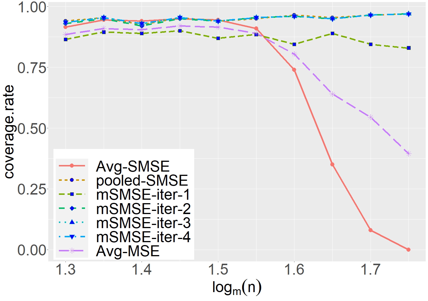
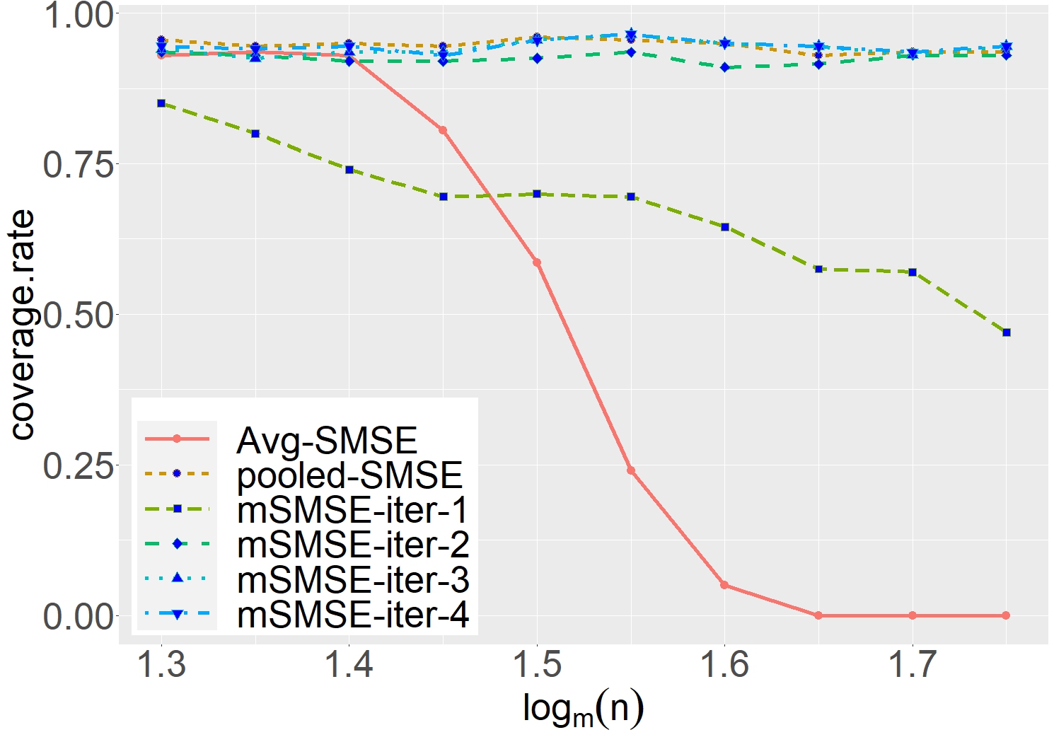
Figure 1 shows the coverage rates as a function of $\log_{m}(n)$ with $p=1$ and $10$. For both cases, our proposed (mSMSE), as well as the pooled estimator, achieves a high coverage rate around 95% no matter how large $\log_{m}(n)$ is, while the two averaging methods both fail when $\log_{m}(n)$ is large, as expected. This is consistent with the findings of Shi et al. (2018). Note that since we fix the local size $m$, increasing $\log_{m}(n)$ is equivalent to increasing $L$, so the failure of averaging methods with large $\log_{m}(n)$ verifies that there exists a restriction on the number of machines, which is illustrated in our theoretical results. Furthermore, we also see that our (mSMSE) algorithm is efficient and stable since the coverage rates of (mSMSE) achieve around 95% in only two iterations and change little in the following third and fourth iterations. In fact, (mSMSE) converges within three iterations in most runs, but we force it to run the fourth iteration to show stability.

5.2 Bias and Variance

In addition, we report the bias and the variance of the estimators with different $\log_{m}(n)$ in Tables 1 and 2. In the tables, when $t\geq 2$, both the bias and the variance of our proposed multi-round method decrease as $n$ increases, and they are close to the bias and the variance of the pooled-SMSE. This is consistent with our theoretical analysis in Section 3.2, where we establish that the bias and the variance of (mSMSE) are both of the rate $n^{-\alpha/(2\alpha+1)}$. On the contrary, the biases of the averaging methods are much larger than the bias of our method and stay large as $n$ increases, as the bias cannot be reduced by averaging in a distributed environment. Note that the bias of (Avg-SMSE) is high since the necessary condition $L=\big{(}m^{2(\alpha-1)/3}\big{)}$ in Theorem 3.1 is violated, as discussed in Section 3.1. While the bias stays large, the variance decreases as $n$ increases, and therefore we observe the failure of inference when $n$ is large for (Avg-MSE) and (Avg-SMSE).

Table 3: The coverage rates (nominal 95%) of (mSMSE) in the first four iterations with different values of $\lambda_{h}$ and $\log_{m}(n)$. The dimension $p=1$ and the noise is homoscedastic normal.

$\lambda_{h}$	$\log_{m}(n)$	$t=1$	$t=2$	$t=3$	$t=4$	$\lambda_{h}$	$\log_{m}(n)$	$t=1$	$t=2$	$t=3$	$t=4$
1	1.35	0.90	0.95	0.96	0.96	10	1.35	0.92	0.93	0.93	0.93
	1.55	0.88	0.96	0.96	0.96		1.55	0.91	0.95	0.95	0.95
	1.75	0.83	0.95	0.95	0.95		1.75	0.89	0.93	0.93	0.93
20	1.35	0.92	0.93	0.93	0.93	$\widehat{\lambda_{h}^{*}}$	1.35	0.91	0.94	0.94	0.94
	1.55	0.90	0.96	0.96	0.96		1.55	0.93	0.95	0.95	0.95
	1.75	0.89	0.94	0.94	0.94		1.75	0.84	0.92	0.94	0.94

5.3 Sensitivity Analysis

In this section, we use numerical experiments to show the sensitivity of the constant $\lambda_{h}$ in the bandwidth $h_{t}$ in Theorem 3.3. An expression of the optimal value of $\lambda_{h}^{*}$ is obtained in (15) to minimize the asymptotic mean squared error. We estimate $\lambda_{h}^{*}$ using $\widehat{U}$, $\widehat{V}$, and $\widehat{V}_{s}$. Under our experiment settings, the estimated constant $\widehat{\lambda^{*}_{h}}$ ranges from 1 to 17 in practice. To study the effect of $\lambda_{h}$ on the validity of inference, we choose a wider range for $\lambda_{h}$, from 1 to 20, and report the coverage rates of the first four iterations of (mSMSE) in Table 3, with different $\lambda_{h}$ and $\log_{m}(n)$. In the first iteration, it seems that larger $\lambda_{h}$’s lead to higher coverage rates, which may indicate that a larger bandwidth improves the initial estimator more aggressively at the beginning of the algorithm. However, after the (mSMSE) converges in two or three iterations, all estimators achieve near-nominal coverage rates, no matter what value $\lambda_{h}$ is. Therefore, (mSMSE) generally allows arbitrary choices of $\lambda_{h}$ in a wide range, which suggests that our proposed (mSMSE) algorithm is robust with respect to $\lambda_{h}$.

5.4 Time Complexity

In this section, we compare the computational complexity of each method. The average CPU times that each method takes when $p=10$ are reported in Table 4. The computation time is recorded in a simulated distributed environment on a RedHat Enterprise Linux cluster containing 524 Lenovo SD650 nodes interconnected by high-speed networks. On each computer node, two Intel Xeon Platinum 8268 24C 205W 2.9GHz Processors are equipped with 48 processing cores.

In Table 4, we first notice that the speed of (mSMSE) is much faster than the pooled estimator and the discrepancy greatly increases when $n$ gets larger. Second, the computation time of (mSMSE) is comparable to (Avg-SMSE). This result may seem counterintuitive since (mSMSE) still requires running an SMSE on the first machine for the initial estimator. However, since the computation time of (Avg-SMSE) is mainly determined by the maximum computation time of the $L$ local machines, (Avg-SMSE) greatly suffers from the computational performance of the “worst” machine, especially when the number of machines is large. On the other hand, (mSMSE) only runs SMSE on one machine and therefore achieves comparable computation time in the experiments.

Table 4: The CPU times (in seconds) that different methods take to compute the estimator, with $p=10$, $\log_{m}(n)$ from 1.35 to 1.75, and homoscedastic normal noise.

$\log_{m}(n)$	(mSMSE) $t=2$	(mSMSE) $t=3$	(Avg-SMSE)	pooled-SMSE
1.35	0.364	0.485	0.307	0.559
1.45	0.365	0.492	0.328	1.356
1.55	0.426	0.605	0.370	3.260
1.65	0.443	0.627	0.399	9.267
1.75	0.474	0.665	0.459	23.208

6 Conclusion and Future Works

In this paper, we study the semi-parametric binary response model in a distributed environment. The problem has been studied in Shi et al. (2018) with the maximum score estimator (Avg-MSE) from the perspective of its statistical properties. We provide two algorithms to achieve faster convergence rates under relaxed constraints on the number of machines $L$: (1) the first approach (Avg-SMSE) is a one-round divide-and-conquer type algorithm on a smoothed objective; (2) the second approach (mSMSE) completely removes the constraints via iterative smoothing in a multi-round procedure. From the statistical perspective, (mSMSE) achieves the optimal non-parametric rate of convergence; from the algorithmic perspective, it achieves quadratic convergence with respect to the number of iterations, up to the statistical error rate. We further provide two generalizations of the problem: how to handle the heterogeneity of datasets with covariate shift and how to translate the problem to high-dimensional settings.

It is worthwhile noting that, in this paper, we assume that the communication of $p\times p$ matrices is allowed in a distributed environment under low-dimensional settings, but not under high-dimensional settings. If the communication of the $p$-dimensional matrix is prohibited in the low-dimensional settings, one may implement our high-dimensional algorithm, which entails a slower algorithmic convergence over the iterations but achieves the same statistical accuracy when the algorithm terminates. Another option that could be considered is using the techniques in Chen et al. (2021) to approximate the second-order information matrix by first-order information, which we leave for future studies.

In addition, the smoothing technique is closely related to other non-parametric and semi-parametric methods such as the change plane problem (Mukherjee et al., 2020) and kernel density estimators (Härdle et al., 2004). We anticipate the multi-round smoothing refinements can be adapted to other such estimators and improve the rate of convergence without a restriction on the number of machines. It is also worthwhile noting that recently a new smoothing method has been proposed for quantile regression (see, e.g., Fernandes et al., 2021; He et al., 2021; Tan et al., 2021; He et al., 2022; Tan et al., 2022). They proposed a specific form of the kernel function to ensure the loss function in the smoothed quantile regression to be strictly convex. It is not clear whether we can devise the choice of $H\left(z/h\right)$ to achieve the same advantage.

Lastly, for the high-dimensional settings, our proposed algorithm is based on the spirit of the Dantzig Selector. A recent paper (Feng et al., 2022) considered a regularized objective and obtained a minimax optimal rate for the linear binary response model. It could be potentially interesting to apply this approach to the maximum score estimator under the distributed setting.

Appendix A Theoretical Results of the High-dimensional (mSMSE)

In this section, we give the complete theoretical analysis of the high-dimensional multi-round SMSE in Algorithm 2. First, we restate the conditions as the following two assumptions.

Assumption 10.

The initial value $\widehat{\bm{\beta}}^{\,\left(0\right)}$ satisfies

$$\left\|\widehat{\bm{\beta}}^{\,\left(0\right)}-\bm{\beta}^{*}\right\|_{2}=O_{\mathbb{P}}\left(\delta_{m,0}\right),\quad\left\|\widehat{\bm{\beta}}^{\,\left(0\right)}-\bm{\beta}^{*}\right\|_{1}=O_{\mathbb{P}}\left(\sqrt{s}\delta_{m,0}\right),$$ (29)

for some $\delta_{m,0}=o(1)$.

Assumption 11.

The dimension $p=O\left(n^{\nu}\right)$ for some $\nu>0$ and the sparsity $s=O\left(m^{r}\right)$ for some $0<r<1/4$.

Assumption 10 requires that the error of the initial value can be upper bounded in both $\ell_{1}$ and $\ell_{2}$ norm. Moreover, the bound of the $\ell_{1}$ error is of the same order as $\sqrt{s}$ times the bound of the $\ell_{2}$ error. This could be achieved by the path-following method proposed by Feng et al. (2022), with $\delta_{m,0}=\left(s\log p/m\right)^{\alpha/(2\alpha+1)}$. Assumption 11 restricts the dimension $p$ and the sparsity $s$. The first constraint $p=O\left(n^{\nu}\right)$ implies that $\log p=O\left(\log n\right)$, so we will simply use $\log p$ instead of $\log\max\left\{n,p\right\}$ in the following theorems. The sparsity condition $s=O\left(m^{r}\right)$ is also necessary and standard to guarantee convergence. Under these assumptions, we formally restate Theorem 4.4:

Theorem A.1.

For $t=1,2,\dots,T$, define $h^{*}:=\left(\log p/n\right)^{1/\left(2\alpha+1\right)}$, $r_{m}:=\sqrt{\frac{s^{2}\log p}{m(h^{*})^{3}}}+s^{3/2}\delta_{m,0}$ and

$$\delta_{m,t}:=\sqrt{s}\left(\frac{\log p}{n}\right)^{\frac{\alpha}{2\alpha+1}}+\left(r_{m}\right)^{t}\delta_{m,0}.$$

Assume the assumptions in Theorem 3.4 and Assumptions 10,11 hold. Then there exists a constant $\alpha_{0}$ such that, by choosing a kernel $H^{\prime}(\cdot)$ with order $\alpha>\alpha_{0}$, bandwidth $h_{t}\equiv h^{*}$ for $t=1,2,\dots,T$ and parameters

$$\lambda^{\left(t\right)}_{n}=C_{\lambda}\left[\left(\frac{\log p}{n}\right)^{\frac{\alpha}{2\alpha+1}}+\sqrt{\frac{s\log p}{m(h^{*})^{3}}}\delta_{m,t-1}+s\delta^{2}_{m,t-1}\right],$$

with a sufficiently large constant $C_{\lambda}$, we have $r_{m}=o(1)$,

$$\left\|\widehat{\bm{\beta}}^{\,\left(t\right)}-\bm{\beta}^{*}\right\|_{2}=O_{\mathbb{P}}\left(\delta_{m,t}\right)\quad{\rm and}\quad\left\|\widehat{\bm{\beta}}^{\,\left(t\right)}-\bm{\beta}^{*}\right\|_{1}\leq 2\sqrt{s}\left\|\widehat{\bm{\beta}}^{\,\left(t\right)}-\bm{\beta}^{*}\right\|_{2},$$ (30)

with probability tending to one.

The proof of Theorem A.1 is given in Section B.5. The $\delta_{m,t}$ in Theorem A.1 denotes the upper bound on the $\ell_{2}$-error of $\widehat{\bm{\beta}}^{(t)}$, which contains two terms. The first term $\sqrt{s}\left(\log p/n\right)^{\alpha/(2\alpha+1)}$ is the best rate our method can achieve and the second term comes from the error of the initial estimator. As long as $r_{m}=o(1)$, the second term decreases exponentially as $t$ increases, which implies that $\widehat{\bm{\beta}}^{(t)}$ achieves the optimal rate after at most $O(\log n)$ iterations. Concretely, the number of required iterations is

$$\frac{\alpha\left[\left(\log n-\log\log n\right)-\frac{1}{2}\log s+\log\delta_{m,0}\right]}{(2\alpha+1)\left[-\log\left(r_{m}\right)\right]},$$ (31)

which is larger than that in the low-dimensional case. Under the Assumption 11 and the assumption $m>n^{c}$ in Theorem 3.4, it’s easy to see that (31) can be upper bounded by a finite number.

The condition $r_{m}=o(1)$ can be ensured by choosing a kernel function with order higher than a constant certain $\alpha_{0}$. See Remark 5 for explanation.

Remark 5.

To make sure that $r_{m}=\frac{s^{2}\log m}{m(h^{*})^{3}}+s^{3/2}\delta_{m,0}=o(1)$ and $\sqrt{s}\delta_{m,0}=O\left(\left(h^{*}\right)^{3/2}\right)$, we need to choose a kernel $H^{\prime}(\cdot)$ with order $\alpha$ such that $\alpha>\alpha_{0}:=\max\left\{\frac{3}{2c\,\left(1-2r\right)}+\frac{r}{2(1-2r)},\frac{3r}{2(1-4r)}\right\}$, where $c=(\log m)/(\log n)<1$ and $r=(\log s)/(\log m)<1/4$ are supposed in Theorem 3.4 and Assumption 11. Here we plug in the rate $\delta_{m,0}=(s\log p/m)^{\alpha/(2\alpha+1)}$ obtained by the path-following algorithm by Feng et al. (2022). If the order of the kernel is not high enough (less than $\alpha_{0}$), Algorithm 2 still works by choosing $h_{m}=m^{-\frac{2\alpha(1-2r)}{3(2\alpha+1)}+\varepsilon}$ for some small $\varepsilon>0$, and the corresponding convergence rate will be $\sqrt{s}h^{\alpha}_{m}$.

Appendix B Technical Proof of the Theoretical Results

B.1 Proof of the Results for the $\ell_{2}$ Error Bound of (mSMSE)

Proof of Proposition 3.2

We first restate Proposition 3.2 in a detailed version. The first step of (mSMSE) can be written as

$$\widehat{\bm{\beta}}^{(1)}-\bm{\beta}^{*}=\Big{(}V_{n,h_{1}}\big{(}\widehat{\bm{\beta}}^{(0)}\big{)}\Big{)}^{-1}U_{n,h_{1}}\big{(}\widehat{\bm{\beta}}^{\left(0\right)}\big{)},$$ (32)

where

$$V_{n,h}\left(\bm{\beta}\right)= \nabla^{2}F_{h}\left(\bm{\beta}\right)=\frac{1}{nh^{2}}\sum_{i=1}^{n}\left(-y_{i}\right)H^{\prime\prime}\left(\frac{x_{i}+\bm{z}_{i}^{\top}\bm{\beta}}{h}\right)\bm{z}_{i}\bm{z}_{i}^{\top},$$ (33)

$$U_{n,h}\left(\bm{\beta}\right)= \frac{1}{nh^{2}}\sum_{i=1}^{n}\left(-y_{i}\right)H^{\prime\prime}\left(\frac{x_{i}+\bm{z}_{i}^{\top}\bm{\beta}}{h}\right)\bm{z}_{i}\bm{z}_{i}^{\top}\left(\bm{\beta}-\bm{\beta}^{*}\right)-\frac{1}{nh}\sum_{i=1}^{n}\left(-y_{i}\right)H^{\prime}\left(\frac{x_{i}+\bm{z}_{i}^{\top}\bm{\beta}}{h}\right)\bm{z}_{i}.$$ (34)

Proposition 3.2.

Assume Assumptions 1–5 hold. Further assume that $\left\lVert\widehat{\bm{\beta}}^{\left(0\right)}-\bm{\beta}^{*}\right\rVert_{2}=O_{\mathbb{P}}\left(\delta_{m,0}\right)$, $\delta_{m,0}=O\left(h_{1}\right)$, $h_{1}=o\left(1\right)$ and $\frac{\log n}{nh_{1}^{3}}=o\left(1\right)$. We have

$$\left\|U_{n,h_{1}}\left(\widehat{\bm{\beta}}^{\,\left(0\right)}\right)\right\|_{2}=O_{\mathbb{P}}\left(\delta_{m,0}^{2}+h_{1}^{\alpha}+\sqrt{\frac{1}{nh_{1}}}+\delta_{m,0}\sqrt{\frac{\log n}{nh_{1}^{3}}}\right),$$ (35)

$$\left\|V_{n,h_{1}}\left(\widehat{\bm{\beta}}^{\,\left(0\right)}\right)-V\right\|_{2}=O_{\mathbb{P}}\left(\sqrt{\frac{\log n}{nh_{1}^{3}}}+\delta_{m,0}+h_{1}\right),$$ (36)

and therefore

$$\left\|\widehat{\bm{\beta}}^{\,\left(1\right)}-\bm{\beta}^{*}\right\|_{2}=O_{\mathbb{P}}\left(\delta_{m,0}^{2}+h_{1}^{\alpha}+\sqrt{\frac{1}{nh_{1}}}+\delta_{m,0}\sqrt{\frac{\log n}{nh_{1}^{3}}}\right).$$ (37)

Proof of Proposition 3.2.

Throughout the whole proof, without loss of generality, we assume that $\left\lVert\widehat{\bm{\beta}}^{\left(0\right)}-\bm{\beta}^{*}\right\rVert_{2}\leq\delta_{m,0}$ with probability approaching one, i.e., we assume the constant in $O_{\mathbb{P}}(\delta_{m,0})$ to be 1. For simplicity, we replace the notation $h_{1}$ with $h$. Also, note that the dimension $p$ is fixed.

Proof of (35)

First prove (35). It suffices to show that

$$\sup_{\bm{\beta}:\left\lVert\bm{\beta}-\bm{\beta}^{*}\right\rVert_{2}\leq\delta_{m,0}}\left\|U_{n,h}\left(\bm{\beta}\right)\right\|_{2}=O_{\mathbb{P}}\left(\delta_{m,0}^{2}+h^{\alpha}+\sqrt{\frac{1}{nh}}+\delta_{m,0}\sqrt{\frac{\log n}{nh^{3}}}\right),$$ (38)

which implies (35) since $\left\lVert\widehat{\bm{\beta}}^{\left(0\right)}-\bm{\beta}^{*}\right\rVert_{2}\leq\delta_{m,0}$ with probability approaching one.

By the proof of Lemma 3 in Cai et al. (2010), there exists $\bm{v}_{1},...,\bm{v}_{5^{p}}\in\mathbb{R}^{p}$, s.t. for any $\bm{v}$ in the unit sphere $\mathbb{S}^{p-1}=\left\{\bm{v}\in\mathbb{R}^{p}:\left\lVert\bm{v}\right\rVert_{2}=1\right\}$, there exists $j_{v}\in[5^{p}]$ satisfying $\left\lVert\bm{v}-\bm{v}_{j_{v}}\right\rVert_{2}\leq 1/2$. Then we have

$$\left\lVert U_{n,h}\left(\bm{\beta}\right)\right\rVert_{2}=\sup_{\bm{v}\in\mathbb{S}^{p-1}}\left\lvert\bm{v}^{\top}U_{n,h}\left(\bm{\beta}\right)\right\rvert\leq\sup_{j_{v}\in[5^{p}]}\left\lvert\bm{v}_{j_{v}}^{\top}U_{n,h}\left(\bm{\beta}\right)\right\rvert+\frac{1}{2}\left\lVert U_{n,h}\left(\bm{\beta}\right)\right\rVert_{2},$$

and thus

$$\left\lVert U_{n,h}\left(\bm{\beta}\right)\right\rVert_{2}\leq\sup_{{j_{v}}\in[5^{p}]}2\left\lvert\bm{v}_{j_{v}}^{\top}U_{n,h}\left(\bm{\beta}\right)\right\rvert.$$

Therefore, to show (38), it suffices to show that

$$\sup_{\bm{\beta}:\left\lVert\bm{\beta}-\bm{\beta}^{*}\right\rVert_{2}\leq\delta_{m,0}}\sup_{{j_{v}}\in[5^{p}]}\left\lvert\bm{v}_{j_{v}}^{\top}U_{n,h}\left(\bm{\beta}\right)\right\rvert=O_{\mathbb{P}}\left(\sqrt{\frac{1}{nh}}+\delta_{m,0}\sqrt{\frac{\log n}{nh^{3}}}+\delta_{m,0}^{2}+h^{\alpha}\right).$$ (39)

From now on, we let $\bm{v}$ be an arbitrarily fixed vector in $\mathbb{S}^{p-1}$. Recall the definition

$$\quad U_{n,h}\left(\bm{\beta}\right)$$

$$=\frac{1}{nh^{2}}\sum_{i=1}^{n}\left(-y_{i}\right)H^{\prime\prime}\left(\frac{x_{i}+\bm{z}_{i}^{\top}\bm{\beta}}{h}\right)\bm{z}_{i}\bm{z}_{i}^{\top}\left(\bm{\beta}-\bm{\beta}^{*}\right)-\frac{1}{nh}\sum_{i=1}^{n}\left(-y_{i}\right)H^{\prime}\left(\frac{x_{i}+\bm{z}_{i}^{\top}\bm{\beta}}{h}\right)\bm{z}_{i}$$

$$=:\frac{1}{n}\sum_{i=1}^{n}U_{h,i}\left(\bm{\beta}\right),$$

where

$$U_{h,i}\left(\bm{\beta}\right):=\frac{1}{h^{2}}\left(-y_{i}\right)H^{\prime\prime}\left(\frac{x_{i}+\bm{z}_{i}^{\top}\bm{\beta}}{h}\right)\bm{z}_{i}\bm{z}_{i}^{\top}\left(\bm{\beta}-\bm{\beta}^{*}\right)-\frac{1}{h}\left(-y_{i}\right)H^{\prime}\left(\frac{x_{i}+\bm{z}_{i}^{\top}\bm{\beta}}{h}\right)\bm{z}_{i}.$$ (40)

We have the following decomposition:

$$\quad\bm{v}^{\top}U_{n,h}\left(\bm{\beta}\right)$$ (41)

$$=(1-\mathbb{E})\left[\bm{v}^{\top}U_{n,h}\left(\bm{\beta}\right)-\bm{v}^{\top}U_{n,h}\left(\bm{\beta}^{*}\right)\right]+(1-\mathbb{E})\bm{v}^{\top}U_{n,h}\left(\bm{\beta}^{*}\right)+\mathbb{E}\bm{v}^{\top}U_{n,h}\left(\bm{\beta}\right)$$

$$=\frac{1}{n}\sum_{i=1}^{n}\phi^{U}_{i}(\bm{\beta})+(1-\mathbb{E})\bm{v}^{\top}U_{n,h}\left(\bm{\beta}^{*}\right)+\mathbb{E}\bm{v}^{\top}U_{n,h}\left(\bm{\beta}\right)$$

where $\phi^{U}_{i}(\bm{\beta}):=(1-\mathbb{E})\left[\bm{v}^{\top}U_{h,i}(\bm{\beta})-\bm{v}^{\top}U_{h,i}(\bm{\beta}^{*})\right]$. We will separately bound the three terms in (41). through the following three steps.

Step 1

We will show that, for some constant $\gamma>0$, there exists $C_{\phi}>0$ such that

$$\sup_{\left\lVert\bm{\beta}-\bm{\beta}^{*}\right\rVert_{2}\leq\delta_{m,0}}\left\lvert\frac{1}{n}\sum_{i=1}^{n}\phi^{U}_{i}(\bm{\beta})\right\rvert\leq C_{\phi}\delta_{m,0}\sqrt{\frac{\log n}{nh^{3}}},$$ (42)

with probability $1-2n^{-\gamma p}$.

For any positive $\gamma$ and each $j\in\left\{1,\dots,p\right\}$, divide the interval $[\beta^{*}_{j}-\delta_{m,0},\beta^{*}_{j}+\delta_{m,0}]$ into $n^{\gamma}$ small intervals, each with length $\frac{2\delta_{m,0}}{n^{\gamma}}$. This division creates $n^{\gamma}$ intervals on each dimension, and the direct product of those intervals divides the hypercube $\left\{\bm{\beta}:\left\lVert\bm{\beta}-\bm{\beta}^{*}\right\rVert_{\infty}\leq\delta_{m,0}\right\}$ into $n^{\gamma p}$ small hypercubes. By arbitrarily picking a point on each small hypercube, we could find $\left\{\bm{\beta}_{1},...,\bm{\beta}_{n^{\gamma p}}\right\}\subset\mathbb{R}^{p}$, such that for all $\bm{\beta}$ in the ball $\left\{\bm{\beta}:\left\lVert\bm{\beta}-\bm{\beta}^{*}\right\rVert_{2}\leq\delta_{m,0}\right\}$ (which is a subset of $\left\{\bm{\beta}:\left\lVert\bm{\beta}-\bm{\beta}^{*}\right\rVert_{\infty}\leq\delta_{m,0}\right\}$), there exists $j_{\beta}\in[n^{\gamma p}]$ such that $\left\lVert\bm{\beta}-\bm{\beta}_{j_{\beta}}\right\rVert_{\infty}\leq\frac{2\delta_{m,0}}{n^{\gamma}}$.

By Assumption 5 which requires $\sup_{i}\left\lVert\bm{z}_{i}\right\rVert_{\infty}\leq\overline{B}$, we have $\left\lvert\bm{v}^{\top}\bm{z}_{i}\right\rvert\leq\overline{B}\left\lVert\bm{v}\right\rVert_{1}\leq\overline{B}\sqrt{p}\left\lVert\bm{v}\right\rVert_{2}$ for any $\bm{v}\in\mathbb{R}^{p}$. By Assumption 1, $H^{\prime\prime}\left(x\right)$, $H^{\prime}\left(x\right)$ are both bounded and Lipschitz continuous, and thus we have

$$\quad\left\lvert\bm{v}^{\top}U_{h,i}(\bm{\beta})-\bm{v}^{\top}U_{h,i}(\bm{\beta}_{j_{\beta}})\right\rvert$$

$$\leq\frac{\left\lvert\bm{v}^{\top}\bm{z}_{i}\right\rvert}{h^{2}}\left\lvert\bm{z}_{i}^{\top}\left(\bm{\beta}-\bm{\beta}^{*}\right)\left[H^{\prime\prime}\left(\frac{x_{i}+\bm{z}_{i}^{\top}\bm{\beta}}{h}\right)-H^{\prime\prime}\left(\frac{x_{i}+\bm{z}_{i}^{\top}\bm{\beta}_{j_{\beta}}}{h}\right)\right]+\bm{z}_{i}^{\top}\left(\bm{\beta}-\bm{\beta}_{j_{\beta}}\right)H^{\prime\prime}\left(\frac{x_{i}+\bm{z}_{i}^{\top}\bm{\beta}_{j_{\beta}}}{h}\right)\right\rvert$$

$$\quad+\frac{\left\lvert\bm{v}^{\top}\bm{z}_{i}\right\rvert}{h}\left\lvert H^{\prime}\left(\frac{x_{i}+\bm{z}_{i}^{\top}\bm{\beta}_{j_{\beta}}}{h}\right)-H^{\prime}\left(\frac{x_{i}+\bm{z}_{i}^{\top}\bm{\beta}}{h}\right)\right\rvert$$

$$\leq C\left(\frac{\overline{B}^{3}p^{3/2}\delta^{2}_{m,0}}{n^{\gamma}h^{3}}+\frac{\overline{B}^{2}p\delta_{m,0}}{n^{\gamma}h^{2}}\right),$$

for some constant $C$ depending on $H$ but not on $\bm{\beta}$ or $\bm{\beta}_{j_{\beta}}$. Therefore,

$$\left\lvert\phi_{i}^{U}(\bm{\beta})-\phi_{i}^{U}\left(\bm{\beta}_{j_{\beta}}\right)\right\rvert\leq\left\lvert(1-\mathbb{E})\left[\bm{v}^{\top}U_{h,i}(\bm{\beta})-\bm{v}^{\top}U_{h,i}(\bm{\beta}_{j_{\beta}})\right]\right\rvert\lesssim\frac{\overline{B}^{3}p^{3/2}\delta^{2}_{m,0}}{n^{\gamma}h^{3}}+\frac{\overline{B}^{2}p\delta_{m,0}}{n^{\gamma}h^{2}},$$

Choose $\gamma$ to be sufficiently large such that

$$\frac{\overline{B}^{3}p^{3/2}\delta^{2}_{m,0}}{n^{\gamma}h^{3}}+\frac{\overline{B}^{2}p\delta_{m,0}}{n^{\gamma}h^{2}}\ll\delta_{m,0}\sqrt{\frac{\log n}{nh^{3}}},$$

and then we have

$$\quad\sup_{\left\lVert\bm{\beta}-\bm{\beta}^{*}\right\rVert_{2}\leq\delta_{m,0}}\left\lvert\frac{1}{n}\sum_{i=1}^{n}\phi^{U}_{i}(\bm{\beta})\right\rvert-\sup_{j_{\beta}\in[n^{\gamma p}]}\left\lvert\frac{1}{n}\sum_{i=1}^{n}\phi^{U}_{i}(\bm{\beta}_{j_{\beta}})\right\rvert$$ (43)

$$=o\left(\delta_{m,0}\sqrt{\frac{\log n}{nh^{3}}}\right).$$

Now let $\bm{\beta}$ be a fixed vector in $\{\bm{\beta}:\left\lVert\bm{\beta}-\bm{\beta}^{*}\right\rVert_{2}\leq\delta_{m,0}\}$. Again using $\left\lvert\bm{v}^{\top}\bm{z}_{i}\right\rvert\leq\overline{B}\sqrt{p}$, $\left\lvert\bm{z}_{i}^{\top}\left(\bm{\beta}-\bm{\beta}^{*}\right)\right\rvert\leq\overline{B}\sqrt{p}\delta_{m,0}$ and the boundedness of $H^{\prime}\left(x\right)$ and $H^{\prime\prime}\left(x\right)$, we have

$$\sup_{i}\left\lvert\phi^{U}_{i}\left(\bm{\beta}\right)\right\rvert=O\left(\frac{\overline{B}^{2}p\delta_{m,0}}{h^{2}}\right),$$ (44)

Recall that $\zeta=X+\bm{Z}^{\top}\bm{\beta}^{*}$ and $\rho\left(\cdot\,|\,\bm{Z}\right)$ denotes the density of $\zeta$ given $\bm{Z}$. Let $\mathbb{E}_{\cdot|\bm{Z}}$ denote the expectation conditional on $\bm{Z}$. By Assumption 2, $\rho\left(\cdot\,|\,\bm{Z}\right)$ is bounded in a neighborhood of zero, and hence we have, when $n$ is large enough,

$$\quad\mathbb{E}_{.|\bm{Z}}\left[H^{\prime\prime}\left(\frac{X+\bm{Z}^{\top}\bm{\beta}}{h}\right)\right]^{2}=\mathbb{E}_{.|\bm{Z}}\left[H^{\prime\prime}\left(\frac{\bm{Z}^{\top}\left(\bm{\beta}-\bm{\beta}^{*}\right)+\zeta}{h}\right)\right]^{2}$$ (45)

$$=h\int_{-1}^{1}H^{\prime\prime}\left(\xi\right)^{2}\rho\left(\xi h-\bm{Z}^{\top}\left(\bm{\beta}-\bm{\beta}^{*}\right)\,|\,\bm{Z}\right)\,{\mathrm{d}}\xi$$

$$=O\left(h\right),$$

where we use that $h=o(1)$ and $\bm{Z}^{\top}(\bm{\beta}-\bm{\beta}^{*})\leq\overline{B}\sqrt{p}\delta_{m,0}=o(1)$. Similarly,

$$\mathbb{E}_{.|\bm{Z}}\left[H^{\prime}\left(\frac{X+\bm{Z}^{\top}\bm{\beta}}{h}\right)-H^{\prime}\left(\frac{X+\bm{Z}^{\top}\bm{\beta}^{*}}{h}\right)\right]^{2} =\mathbb{E}_{.|\bm{Z}}\left[\frac{\bm{Z}^{\top}(\bm{\beta}-\bm{\beta}^{*})}{h}H^{\prime\prime}\left(\frac{X+\bm{Z}^{\top}\breve{\bm{\beta}}}{h}\right)\right]^{2}$$ (46)

$$=O\left(\frac{\overline{B}^{2}p\delta_{m,0}^{2}}{h}\right).$$

By (45) and (46),

$$\mathrm{var}\left(\phi^{U}_{i}\left(\bm{\beta}\right)\right) \leq\mathbb{E}\left(\bm{v}^{\top}U_{h,i}\left(\bm{\beta}\right)-\bm{v}^{\top}U_{h,i}(\bm{\beta}^{*})\right)^{2}$$ (47)

$$=O\left(\frac{\overline{B}^{4}p^{2}\delta^{2}_{m,0}}{h^{3}}\right).$$

Neither of the constant hidden in the big O notation of (44) or (47) depends on $\bm{\beta}$. By (44) and (47), we can apply Bernstein inequality to show that there exists a large enough $C_{1}>0$, which does not depend on $\bm{\beta}$, such that

$$\mathbb{P}\left(\left\lvert\frac{1}{n}\sum_{i=1}^{n}\phi^{U}_{i}\left(\bm{\beta}\right)\right\rvert>C_{1}\delta_{m,0}\sqrt{\frac{\log n}{nh^{3}}}\right)\leq 2n^{-2\gamma p}.$$

The above inequality is true for any $\bm{\beta}\in\mathbb{R}^{p}$ that satisfies $\left\lVert\bm{\beta}-\bm{\beta}^{*}\right\rVert_{2}\leq\delta_{m,0}$. In particular, for any $j_{\beta}\in[n^{\gamma p}]$, with probability at least $1-2n^{-2\gamma p}$,

$$\left\lvert\frac{1}{n}\sum_{i=1}^{n}\phi^{U}_{i}\left(\bm{\beta}_{j_{\beta}}\right)\right\rvert\leq C_{1}\delta_{m,0}\sqrt{\frac{\log n}{nh^{3}}},$$

which implies that with probability at least $1-2n^{-\gamma p}$,

$$\sup_{j_{\beta}\in[n^{\gamma p}]}\left\lvert\frac{1}{n}\sum_{i=1}^{n}\phi^{U}_{i}(\bm{\beta}_{j_{\beta}})\right\rvert\leq C_{1}\delta_{m,0}\sqrt{\frac{\log n}{nh^{3}}}.$$

Combining with (43), we obtain (42).

Step 2 We will show that there exists a constant $C^{*}>0$, such that

$$(1-\mathbb{E})\bm{v}^{\top}U_{n,h}\left(\bm{\beta}^{*}\right)\geq C^{*}\sqrt{\frac{1}{nh}},$$ (48)

with probability at least $1-2n^{-\gamma p}$, where $\gamma$ has been specified in Step 1.

Note that $(1-\mathbb{E})\bm{v}^{\top}U_{n,h}\left(\bm{\beta}^{*}\right)=\frac{1}{n}\sum_{i=1}^{n}(1-\mathbb{E})\left[\bm{v}^{\top}U_{h,i}\left(\bm{\beta}^{*}\right)\right]$ and $(1-\mathbb{E})\left[\bm{v}^{\top}U_{h,i}\left(\bm{\beta}^{*}\right)\right]$ are i.i.d. among different $i$. By Assumption 2, the density function of $\zeta=X+\bm{Z}^{\top}\bm{\beta}^{*}$ satisfies that $\rho^{(1)}(\cdot\,|\,\bm{Z})$ is bounded uniformly for all $\bm{Z}$ in a neighborhood of 0, which implies that $\rho(t\,|\,Z)=\rho(0\,|\,\bm{Z})+O(t)$. The constant in $O(t)$ is the same for all $t$ in the neighborhood. Therefore,

$$\mathbb{E}_{\cdot\,|\,\bm{Z}}\left[\bm{v}^{\top}U_{h,i}\left(\bm{\beta}^{*}\right)\right]^{2}$$ (49)

$$= \frac{\left(\bm{v}^{\top}\bm{Z}\right)^{2}}{h^{2}}\mathbb{E}_{\cdot\,|\,\bm{Z}}\left[H^{\prime}\left(\frac{X+\bm{Z}^{\top}\bm{\beta}^{*}}{h}\right)\right]^{2}$$

$$= \int_{-1}^{1}\frac{\left(\bm{v}^{\top}\bm{Z}\right)^{2}}{h}\left[H^{\prime}\left(\xi\right)\right]^{2}\rho\left(\xi h\,|\,\bm{Z}\right)\,{\mathrm{d}}\xi$$

$$= \frac{\left(\bm{v}^{\top}\bm{Z}\right)^{2}}{h}\int_{-1}^{1}\left[H^{\prime}\left(\xi\right)\right]^{2}\rho\left(0\,|\,\bm{Z}\right)\,{\mathrm{d}}\xi+O\left((\bm{v}^{\top}\bm{Z})^{2}\right).$$

Recall that $V_{s}:=\pi_{V}\mathbb{E}\rho\left(0\,|\,\bm{Z}\right)\bm{Z}\bm{Z}^{\top}$ and $\pi_{V}:=\int_{-1}^{1}\left[H^{\prime}\left(\xi\right)\right]^{2}\,{\mathrm{d}}\xi$, which leads to

$$\mathbb{E}\left[\bm{v}^{\top}U_{h,i}\left(\bm{\beta}^{*}\right)\right]^{2}=\frac{1}{h}\left(\bm{v}^{\top}V_{s}\bm{v}+O\left(h\right)\right).$$

In Step 3, we also show that $\sup_{\bm{\beta}:\left\lVert\bm{\beta}-\bm{\beta}^{*}\right\rVert_{2}\leq\delta_{m,0}}\mathbb{E}\left[\bm{v}^{\top}U_{h,i}\left(\bm{\beta}\right)\right]=o(1)$. Therefore,

$$\quad\mathrm{var}\left[\sqrt{h}\bm{v}^{\top}U_{h,i}\left(\bm{\beta}^{*}\right)\right]$$ (50)

$$=h\left\{\mathbb{E}\left[\bm{v}^{\top}U_{h,i}\left(\bm{\beta}^{*}\right)\right]^{2}-\left(\mathbb{E}\left[\bm{v}^{\top}U_{h,i}\left(\bm{\beta}^{*}\right)\right]\right)^{2}\right\}$$

$$=\bm{v}^{\top}V_{s}\bm{v}+o\left(1\right),$$

By CLT and Slusky’s Theorem,

$$\sqrt{nh}\left(1-\mathbb{E}\right)\left[\bm{v}^{\top}U_{n,h}\left(\bm{\beta}^{*}\right)\right]\stackrel{{\scriptstyle d}}{{\longrightarrow}}\mathcal{N}\left(0,\bm{v}^{\top}V_{s}\bm{v}\right),$$

which implies (48).

Step 3

We will show that,

$$\sup_{\bm{\beta}:\left\lVert\bm{\beta}-\bm{\beta}^{*}\right\rVert_{2}\leq\delta_{m,0}}\mathbb{E}\left[\bm{v}^{\top}U_{n,h}\left(\bm{\beta}\right)\right]\leq C_{E}(\delta_{m,0}^{2}+h^{\alpha}),$$ (51)

where $C_{E}$ does not depend on $\bm{v}$.

By Assumption 2 and 3, for almost every $\bm{Z}$,

$$\rho\left(t\,|\,\bm{Z}\right)=\sum_{k=0}^{\alpha-1}\frac{1}{k!}\rho^{\,\left(k\right)}\left(0\,|\,\bm{Z}\right)t^{k}+\frac{1}{\alpha!}\rho^{\left(\alpha\right)}\left(t^{\prime}\,|\,\bm{Z}\right)t^{\alpha},$$

$$F\left(-t\,|\,\bm{Z}\right)=\frac{1}{2}+\sum_{k=1}^{\alpha}\frac{1}{k!}F^{\,\left(k\right)}\left(0\,|\,\bm{Z}\right)(-t)^{k}+\frac{1}{\left(\alpha+1\right)!}F^{\left(\alpha+1\right)}\left(t^{\prime\prime}\,|\,\bm{Z}\right)(-t)^{\alpha+1},$$

where $t^{\prime},t^{\prime\prime}$ are between 0 and $t$. Therefore,

$$\left(2F\left(-t\,|\,\bm{Z}\right)-1\right)\rho\left(t\,|\,\bm{Z}\right)=\sum_{k=1}^{2\alpha+1}M_{k}\left(\bm{Z}\right)t^{k},$$ (52)

where $M_{k}\left(\bm{Z}\right)$’s are constants depending on $\rho$, $F$, $\bm{Z}$, and $t$. Since $\rho^{\left(k\right)}\left(\cdot\,|\,\bm{Z}\right)$ and $F^{\left(k\right)}\left(\cdot\,|\,\bm{Z}\right)$ are bounded around 0 for all $k$ and $\bm{Z}$, we know there exists a constant $M$ such that $\sup_{k,\bm{Z},t}\left\lvert M_{k}\left(\bm{Z}\right)\right\rvert\leq M$ for all $t$ in a certain neighborhood of 0.

(In particular,

$$M_{\alpha}\left(\bm{Z}\right)=\sum_{k=1}^{\alpha}\frac{2(-1)^{-k}}{\left(\alpha-k\right)!k!}F^{\,\left(k\right)}\left(0\,|\,\bm{Z}\right)\rho^{\,\left(\alpha-k\right)}\left(0\,|\,\bm{Z}\right),$$

which will be used in the proof of Theorem 3.4.)

By Assumption 1, when $x>1$ or $x<-1$, $H^{\prime}\left(x\right)=H^{\prime\prime}\left(x\right)=0$. The kernel $H^{\prime}\left(x\right)=\int_{-1}^{x}H^{\prime\prime}\left(t\right)\,{\mathrm{d}}t$ is bounded, satisfying $\int_{-1}^{1}H^{\prime}\left(x\right)\,{\mathrm{d}}x=1$ and $\int_{-1}^{1}x^{k}H^{\prime}\left(x\right)\,{\mathrm{d}}x=0$ for any $1\leq k\leq\alpha-1$. Using integration by parts, we have $\int_{-1}^{1}xH^{\prime\prime}\left(x\right)\,{\mathrm{d}}x=-1$ and $\int_{-1}^{1}x^{k}H^{\prime\prime}\left(x\right)\,{\mathrm{d}}x=0$ for $k=0$ and $2\leq k\leq\alpha$.

Now we are ready to compute the expectation of $\bm{v}^{\top}U_{n,h}\left(\bm{\beta}\right)$. Since $\mathbb{E}\left[\bm{v}^{\top}U_{n,h}\left(\bm{\beta}\right)\right]=\mathbb{E}\left[\bm{v}^{\top}U_{h,i}\left(\bm{\beta}\right)\right]$ for all $i$, we omit $i$ in the following computation of expectation. Let $\mathbb{E}_{\cdot|\bm{Z}}$ denote the expectation conditional on $\bm{Z}$. Define $\Delta\left(\bm{\beta}\right):=\bm{\beta}-\bm{\beta}^{*}$ and recall that $\zeta=X+\bm{Z}^{\top}\bm{\beta}^{*}$.

$$\mathbb{E}_{\cdot|\bm{Z}}\left[\bm{v}^{\top}U_{n,h}\left(\bm{\beta}\right)\right]$$ (53)

$$= \bm{Z}^{\top}\bm{v}\cdot\mathbb{E}_{\cdot|\bm{Z}}\bigg{[}\frac{\bm{Z}^{\top}\Delta\left(\bm{\beta}\right)}{h^{2}}\left[2\mathbb{I}\left(X+\bm{Z}^{\top}\bm{\beta}^{*}+\epsilon<0\right)-1\right]H^{\prime\prime}\left(\frac{X+\bm{Z}^{\top}\bm{\beta}}{h}\right)$$

$$\quad\quad\quad\quad\quad-\frac{1}{h}\left[2\mathbb{I}\left(X+\bm{Z}^{\top}\bm{\beta}^{*}+\epsilon<0\right)-1\right]H^{\prime}\left(\frac{X+\bm{Z}^{\top}\bm{\beta}}{h}\right)\bigg{]}$$

$$= \bm{Z}^{\top}\bm{\bm{v}}\cdot\mathbb{E}_{\cdot|\bm{Z}}\left\{\left[2\mathbb{I}\left(\zeta+\epsilon<0\right)-1\right]\left[\frac{\bm{Z}^{\top}\Delta\left(\bm{\beta}\right)}{h^{2}}H^{\prime\prime}\left(\frac{\zeta+\bm{Z}^{\top}\Delta\left(\bm{\beta}\right)}{h}\right)-\frac{1}{h}H^{\prime}\left(\frac{\zeta+\bm{Z}^{\top}\Delta\left(\bm{\beta}\right)}{h}\right)\right]\right\}$$

$$= \left(\bm{Z}^{\top}\bm{v}\right)\int_{-1}^{1}\left[2F\left(\bm{Z}^{\top}\Delta\left(\bm{\beta}\right)-\xi h\,|\,\bm{Z}\right)-1\right]\rho\left(\xi h-\bm{Z}^{\top}\Delta\left(\bm{\beta}\right)\,|\,\bm{Z}\right)$$

$$\quad\cdot\left(\frac{\bm{Z}^{\top}\Delta\left(\bm{\beta}\right)}{h}H^{\prime\prime}\left(\xi\right)-H^{\prime}\left(\xi\right)\right)\,{\mathrm{d}}\xi\quad\left(\mathrm{by\,changing\,variable\,}\xi=\frac{\zeta+\bm{Z}^{\top}\Delta\left(\bm{\beta}\right)}{h}\right)$$

$$= \,\left(\bm{Z}^{\top}\bm{v}\right)\sum_{k=1}^{2\alpha+1}M_{k}\left(\bm{Z}\right)\int_{-1}^{1}\left(\xi h-\bm{Z}^{\top}\Delta\left(\bm{\beta}\right)\right)^{k}\left(\frac{\bm{Z}^{\top}\Delta\left(\bm{\beta}\right)}{h}H^{\prime\prime}\left(\xi\right)-H^{\prime}\left(\xi\right)\right)\,{\mathrm{d}}\xi.$$

When $1\leq k\leq\alpha-1$,

$$\int_{-1}^{1}\left(\xi h-\bm{Z}^{\top}\Delta\left(\bm{\beta}\right)\right)^{k}\left(\frac{\bm{Z}^{\top}\Delta\left(\bm{\beta}\right)}{h}H^{\prime\prime}\left(\xi\right)-H^{\prime}\left(\xi\right)\right)\,{\mathrm{d}}\xi$$ (54)

$$= \sum_{k^{\prime}=0}^{k}\binom{k}{k^{\prime}}h^{k^{\prime}}\left(-\bm{Z}^{\top}\Delta\left(\bm{\beta}\right)\right)^{k-k^{\prime}}\left[\left(\bm{Z}^{\top}\Delta\left(\bm{\beta}\right)/h\right)\int_{-1}^{1}\xi^{k^{\prime}}H^{\prime\prime}\left(\xi\right)\,{\mathrm{d}}\xi-\int_{-1}^{1}\xi^{k^{\prime}}H^{\prime}\left(\xi\right)\,{\mathrm{d}}\xi\right]$$

$$= \,\left(k-1\right)\left(-\bm{Z}^{\top}\Delta\left(\bm{\beta}\right)\right)^{k},$$

$$\text{When \, }k=\alpha,$$

$$\int_{-1}^{1}\left(\xi h-\bm{Z}^{\top}\Delta\left(\bm{\beta}\right)\right)^{\alpha}\left(\frac{\bm{Z}^{\top}\Delta\left(\bm{\beta}\right)}{h}H^{\prime\prime}\left(\xi\right)-H^{\prime}\left(\xi\right)\right)\,{\mathrm{d}}\xi$$

$$= \sum_{k^{\prime}=0}^{\alpha}\binom{\alpha}{k^{\prime}}h^{k^{\prime}}\left(-\bm{Z}^{\top}\Delta\left(\bm{\beta}\right)\right)^{\alpha-k^{\prime}}\left[\left(\bm{Z}^{\top}\Delta\left(\bm{\beta}\right)/h\right)\int_{-1}^{1}\xi^{k^{\prime}}H^{\prime\prime}\left(\xi\right)\,{\mathrm{d}}\xi-\int_{-1}^{1}\xi^{k^{\prime}}H^{\prime}\left(\xi\right)\,{\mathrm{d}}\xi\right]$$

$$= \,\left(\alpha-1\right)\left(-\bm{Z}^{\top}\Delta\left(\bm{\beta}\right)\right)^{\alpha}-\pi_{U}h^{\alpha},$$

where $\pi_{U}=\int_{-1}^{1}\xi^{\alpha}H^{\prime}\left(\xi\right)\,{\mathrm{d}}\xi$ is defined in Assumption 1.

When $\alpha+1\leq k\leq 2\alpha+1$, using $\left\lvert\bm{Z}^{\top}\Delta\left(\bm{\beta}\right)\right\rvert\leq\overline{B}\sqrt{p}\delta_{m,0}$, $\delta_{m,0}=O(h)$ and that $H^{\prime},H^{\prime\prime}$ are both bounded, we have

$$\sup_{\bm{\beta}:\left\lVert\bm{\beta}-\bm{\beta}^{*}\right\rVert_{2}\leq\delta_{m,0}}\left\lvert\int_{-1}^{1}\left(\xi h-\bm{Z}^{\top}\Delta\left(\bm{\beta}\right)\right)^{k}\left(\frac{\bm{Z}^{\top}\Delta\left(\bm{\beta}\right)}{h}H^{\prime\prime}\left(\xi\right)-H^{\prime}\left(\xi\right)\right)\,{\mathrm{d}}\xi\right\rvert=O\left[h^{\alpha+1}+\delta_{m,0}^{\alpha+1}\right].$$

Since $M_{k}(\bm{Z})$’s are uniformly bounded, we finally obtain

$$\sup_{\bm{\beta}:\left\lVert\bm{\beta}-\bm{\beta}^{*}\right\rVert_{2}\leq\delta_{m,0}}\left\lvert\mathbb{E}\left[\bm{v}^{\top}U_{n,h}\left(\bm{\beta}\right)\right]\right\rvert=O\left(\delta_{m,0}^{2}+h^{\alpha}\right),$$ (55)

which leads to (51).

Combining the three steps leads to, for any fixed vector $\bm{v}\in\mathbb{S}^{p-1}$, there exists a constant $C_{\bm{v}}$, with probability at least $1-4\left(n^{-\gamma}\right)^{p}$,

$$\sup_{\bm{\beta}:\left\lVert\bm{\beta}-\bm{\beta}^{*}\right\rVert_{2}\leq\delta_{m,0}}\left\lvert\bm{v}^{\top}U_{n,h}\left(\bm{\beta}\right)\right\rvert\leq C_{\bm{v}}\left(\sqrt{\frac{1}{nh}}+\delta_{m,0}\sqrt{\frac{\log n}{nh^{3}}}+\delta_{m,0}^{2}+h^{\alpha}\right),$$

The constant $C_{\bm{v}}$ depends on $\bm{v}$. Recall in equation (39), we only consider finite number of $\bm{v}$’s. Take $C_{\sup}=\sup_{j\in[5^{p}]}C_{\bm{v}_{j}}$, and then we have

$$\sup_{\bm{\beta}:\left\lVert\bm{\beta}-\bm{\beta}^{*}\right\rVert_{2}\leq\delta_{m,0}}\sup_{{j_{v}}\in[5^{p}]}\left\lvert\bm{v}_{j_{v}}^{\top}U_{n,h}\left(\bm{\beta}\right)\right\rvert\leq C_{\sup}\left(\sqrt{\frac{1}{nh}}+\delta_{m,0}\sqrt{\frac{\log n}{nh^{3}}}+\delta_{m,0}^{2}+h^{\alpha}\right),$$

with probability at least $1-4(5n^{-\gamma})^{p}$. This proves (38) and completes the proof of (35).

Proof of (36)

The proof of (36) is similar. We will use the same $\bm{v}_{j_{v}}$ and $\bm{\beta}_{j_{\beta}}$ as before. By the proof of Lemma 3 in Cai et al. (2010),

$$\left\lVert A\right\rVert_{2}\leq 4\sup_{{j_{v}}\in[5^{p}]}\left\lvert\bm{v}^{\top}_{j_{v}}A\bm{v}_{j_{v}}\right\rvert,$$

for any symmetric $A\in\mathbb{R}^{p\times p}$. Therefore, we only need to bound $\sup_{{j_{v}}\in[5^{p}]}\left\lvert\bm{v}^{\top}_{j_{v}}\left[V_{n,h}\left(\bm{\beta}^{\left(0\right)}\right)-V\right]\bm{v}_{j_{v}}\right\rvert$. By the choice of $\left\{\bm{\beta}_{j_{\beta}}\right\}$, for all $\bm{\beta}$ in the ball $\left\{\bm{\beta}:\left\lVert\bm{\beta}-\bm{\beta}^{*}\right\rVert_{2}\leq\delta_{m,0}\right\}$, there exists $j_{\beta}\in[n^{\gamma p}]$ such that $\left\lVert\bm{\beta}-\bm{\beta}_{j_{\beta}}\right\rVert_{\infty}\leq\frac{2\delta_{m,0}}{n^{\gamma}}$. Recall

$$V_{n,h}\left(\bm{\beta}\right)=\frac{1}{nh^{2}}\sum_{i=1}^{n}\left(-y_{i}\right)H^{\prime\prime}\left(\frac{x_{i}+\bm{z}_{i}^{\top}\bm{\beta}}{h}\right)\bm{z}_{i}\bm{z}_{i}^{\top}=:\frac{1}{n}\sum_{i=1}^{n}V_{h,i}\left(\bm{\beta}\right),$$

where

$$V_{h,i}\left(\bm{\beta}\right):=\frac{1}{h^{2}}\left(-y_{i}\right)H^{\prime\prime}\left(\frac{x_{i}+\bm{z}_{i}^{\top}\bm{\beta}}{h}\right)\bm{z}_{i}\bm{z}_{i}^{\top}.$$ (56)

We have

$$\left\lvert\bm{v}_{j_{v}}^{\top}V_{n,h}\left(\bm{\beta}\right)\bm{v}_{j_{v}}-\bm{v}_{j_{v}}^{\top}V_{n,h}\left(\bm{\beta}_{j_{\beta}}\right)\bm{v}_{j_{v}}\right\rvert\leq\sup_{i}\frac{\left(\bm{z}_{i}^{\top}\bm{v}_{j_{v}}\right)^{2}}{h^{3}}\bm{z}_{i}^{\top}\left(\bm{\beta}-\bm{\beta}_{j_{\beta}}\right)=O\left(\frac{\overline{B}^{3}p^{3/2}\delta_{m,0}}{n^{\gamma}h^{3}}\right).$$

By taking $\gamma>0$ large enough, it suffices to show that

$$\sup_{{j_{v}}\in[5^{p}]}\sup_{j_{\beta}\in[n^{\gamma p}]}\left\lvert\bm{v}^{\top}_{j_{v}}\left[V_{n,h}\left(\bm{\beta}_{j_{\beta}}\right)-V\right]\bm{v}_{j_{v}}\right\rvert=O_{\mathbb{P}}\left(\sqrt{\frac{\log n}{nh^{3}}}+\delta_{m,0}+h\right).$$

In the following proof, we will again consider any fixed $\bm{\beta}\in\mathbb{R}^{p},\bm{v}\in\mathbb{R}^{p}$ that satisfy $\left\lVert\bm{\beta}-\bm{\beta}^{*}\right\rVert_{2}\leq\delta_{m,0}$ and $\left\lVert\bm{v}\right\rVert_{2}=1$, and then apply the result to the specific $\bm{v}_{j_{v}}$ and $\bm{\beta}_{j_{\beta}}$. The computation of $\mathbb{E}\left[\bm{v}^{\top}\left[V_{n,h}\left(\bm{\beta}\right)-V\right]\bm{v}\right]$ is similar to before, but this time we only need the following expansion:

$$\rho\left(t\,|\,\bm{Z}\right)=\rho\left(0\,|\,\bm{Z}\right)+O\left(t\right),$$

$$F\left(-t\,|\,\bm{Z}\right)=1/2-F^{\prime}\left(0\,|\,\bm{Z}\right)t+O\left(t^{2}\right).$$

Recall that $\int_{-1}^{1}xH^{\prime\prime}\left(x\right)\,{\mathrm{d}}x=-1$ and $\int_{-1}^{1}x^{k}H^{\prime\prime}\left(x\right)\,{\mathrm{d}}x=0$ for $k=0$ and $2\leq k\leq\alpha$.

$$\mathbb{E}_{\cdot|\bm{Z}}\left(\bm{v}^{\top}V_{n,h}\left(\bm{\beta}\right)\bm{v}\right)$$ (57)

$$= \frac{\left(\bm{v}^{\top}\bm{z}\right)^{2}}{h^{2}}\mathbb{E}_{\cdot|\bm{Z}}\left[2\mathbb{I}\left(\zeta+\epsilon<0\right)-1\right]H^{\prime\prime}\left(\frac{\bm{Z}^{\top}\Delta\left(\bm{\beta}\right)+\zeta}{h}\right)$$

$$= \frac{\left(\bm{v}^{\top}\bm{Z}\right)^{2}}{h}\int_{-1}^{1}\left(2F\left(\bm{Z}^{\top}\Delta\left(\bm{\beta}\right)-\xi h\,|\,\bm{Z}\right)-1\right)\rho\left(\xi h-\bm{Z}^{\top}\Delta\left(\bm{\beta}\right)\,|\,\bm{Z}\right)H^{\prime\prime}\left(\xi\right)\,{\mathrm{d}}\xi$$

$$= -2\left(\bm{v}^{\top}\bm{Z}\right)^{2}F^{\prime}\left(0\,|\,\bm{Z}\right)\rho\left(0\,|\,\bm{Z}\right)\int_{-1}^{1}\xi H^{\prime\prime}\left(\xi\right)\,{\mathrm{d}}\xi+O\left(h+\left\lvert\bm{Z}^{\top}\Delta\left(\bm{\beta}\right)\right\rvert^{2}/h\right)$$

$$= 2\left(\bm{v}^{\top}\bm{Z}\right)^{2}F^{\prime}\left(0\,|\,\bm{Z}\right)\rho\left(0\,|\,\bm{Z}\right)+O\left(h+\delta_{m,0}\right),$$

hence

$$\mathbb{E}\left(\bm{v}^{\top}\left[V_{n,h}\left(\bm{\beta}\right)-V\right]\bm{v}\right)=O\left(\delta_{m,0}+h\right).$$ (58)

Since $H^{\prime\prime}\left(x\right)$ is bounded and $\left\lvert\bm{v}^{\top}\bm{z}_{i}\right\rvert\leq\overline{B}\sqrt{p}$ ($p$ is fixed), we have

$$\left\lvert\bm{v}^{\top}V_{h,i}\left(\bm{\beta}\right)\bm{v}\right\rvert=O\left(\frac{1}{h^{2}}\right).$$ (59)

Adding (45), we also have

$$\mathbb{E}\left(\bm{v}^{\top}V_{h,i}\left(\bm{\beta}\right)\bm{v}\right)^{2}\leq\mathbb{E}\left[\frac{\left(\bm{v}^{\top}\bm{z}_{i}\right)^{4}}{h^{4}}O\left(h\right)\right]=O\left(\frac{1}{h^{3}}\right).$$ (60)

By (59) and (60), we could apply Bernstein inequality to show that

$$\mathbb{P}\left(\left\lvert\left(1-\mathbb{E}\right)\frac{1}{n}\sum_{i=1}^{n}\bm{v}^{\top}V_{h,i}\left(\bm{\beta}\right)\bm{v}\right\rvert>C_{2}\sqrt{\frac{p\log n}{nh^{3}}}\right)\leq 2n^{-2\gamma p},$$

for some constant $C_{2}>0$. By the same procedure in the proof of (35), we obtain, with probability at least $1-2\left(5n^{-\gamma}\right)^{p}$,

$$\sup_{j_{\beta}\in[n^{\gamma p}]}\sup_{j_{v}\in[5^{p}]}\left\lvert\bm{v}_{j_{v}}^{\top}\left(V_{n,h}\left(\bm{\beta}_{j_{\beta}}\right)-V\right)\bm{v}_{j_{v}}\right\rvert=O\left(\sqrt{\frac{\log n}{nh^{3}}}+\delta_{m,0}+h\right),$$

which completes the proof of (36).

Finally, (32), (35), and (36) directly leads to (11), given the assumption that $\Lambda_{\min}\left(V\right)>c_{1}^{-1}$ for some $c_{1}>0$ (Assumption 4).

∎

Proof of Theorem 3.3

Proof.

Without loss of generality, we assume $\lambda_{h}=1$. Then we have

$$h_{t}=\max\{n^{-1/(2\alpha+1)},m^{-2^{t}/(3\alpha)}\}\geq n^{-\frac{1}{2\alpha+1}},$$

which implies the assumption $\frac{\log n}{nh^{3}_{t}}=o(1)$ holds for any $t$, since $\frac{\log n}{nh^{3}_{t}}\leq\log n\cdot{n}^{-\frac{2\alpha-2}{2\alpha+1}}\to 0$ if $\alpha>1$. Moreover, for any $t$, $h^{\alpha}_{t}=\max\left\{m^{-2^{t}/3},n^{-\alpha/(2\alpha+1)}\right\}$ and $1/\sqrt{nh_{t}}\leq n^{-\alpha/(2\alpha+1)}$.

We first show that, for any $t$,

$$\left\|\widehat{\bm{\beta}}^{\,\left(t\right)}-\bm{\beta}^{*}\right\|_{2}=O_{\mathbb{P}}\left(n^{-\alpha/(2\alpha+1)}\sqrt{\log n}+m^{-2^{t}/3}\right).$$ (61)

Recall that by (11), if $\left\lVert\widehat{\bm{\beta}}^{(t-1)}-\bm{\beta}^{*}\right\rVert_{2}=O_{\mathbb{P}}\left(\delta_{m,t-1}\right)$ and $\delta_{m,t-1}=O(h_{t})$, we have that

$$\left\|\widehat{\bm{\beta}}^{\,\left(t\right)}-\bm{\beta}^{*}\right\|_{2}=O_{\mathbb{P}}\Bigg{(}\delta_{m,t-1}^{2}+h_{t}^{\alpha}+\sqrt{\frac{1}{nh_{t}}}+\delta_{m,t-1}\sqrt{\frac{\log n}{nh_{t}^{3}}}\Bigg{)},$$ (62)

which implies that

$$\left\|\widehat{\bm{\beta}}^{\,\left(t\right)}-\bm{\beta}^{*}\right\|_{2}=O_{\mathbb{P}}\Bigg{(}\delta_{m,t-1}^{2}+h_{t}^{\alpha}+\sqrt{\frac{\log n}{nh_{t}}}\Bigg{)},$$ (63)

since $\delta_{m,t-1}\sqrt{\frac{\log n}{nh_{t}^{3}}}=O\big{(}\sqrt{\frac{\log n}{nh_{t}}}\big{)}$.

When $t=1$, $\delta_{m,0}:=m^{-1/3}\leq h_{1}=m^{-\frac{2}{3\alpha}}$, which verifies $\delta_{m,0}=O\left(h_{1}\right)$. Then (61) holds since

$$\left\|\widehat{\bm{\beta}}^{\,\left(1\right)}-\bm{\beta}^{*}\right\|_{2}=O_{\mathbb{P}}\left(\sqrt{\frac{\log n}{nh_{1}}}+m^{-2/3}+h_{1}^{\alpha}\right)=O_{\mathbb{P}}\left(n^{-\alpha/(2\alpha+1)}\sqrt{\log n}+m^{-2/3}\right).$$

Assume (61) holds for $t-1$, i.e.,

$$\left\|\widehat{\bm{\beta}}^{\,\left(t-1\right)}-\bm{\beta}^{*}\right\|_{2}=O_{\mathbb{P}}\left(n^{-\alpha/(2\alpha+1)}\sqrt{\log n}+m^{-2^{t-1}/3}\right).$$

Then $\delta_{m,t-1}=n^{-\alpha/(2\alpha+1)}\sqrt{\log n}+m^{-2^{t-1}/3}$. Since $n^{-\alpha/(2\alpha+1)}\sqrt{\log n}\ll n^{-\frac{1}{2\alpha+1}}\leq h_{t}$ and $m^{-2^{t-1}/3}\leq m^{-\frac{2^{t}}{3\alpha}}\leq h_{t}$, it holds that $\delta_{m,t-1}=O\left(h_{t}\right)$. Then by (63),

$$\left\|\widehat{\bm{\beta}}^{\,\left(t\right)}-\bm{\beta}^{*}\right\|_{2}=O_{\mathbb{P}}\left(\sqrt{\frac{\log n}{nh_{t}}}+\delta_{m,t-1}^{2}+h_{t}^{\alpha}\right)=O_{\mathbb{P}}\left(n^{-\alpha/(2\alpha+1)}\sqrt{\log n}+m^{-2^{t}/3}\right),$$

since $h^{\alpha}_{t}=\max\left\{m^{-2^{t}/3},n^{-\alpha/(2\alpha+1)}\right\}$ and $1/\sqrt{nh_{t}}\leq n^{-\alpha/(2\alpha+1)}$. Therefore, we have proved that (61) holds for all $t$ by induction.

To see (12), note that plugging $\delta_{m,t-1}=n^{-\alpha/(2\alpha+1)}\sqrt{\log n}+m^{-2^{t-1}/3}$ into (62) yields that

$$\left\|\widehat{\bm{\beta}}^{\,\left(t\right)}-\bm{\beta}^{*}\right\|_{2}=O_{\mathbb{P}}\Bigg{(}\frac{\log n}{n^{2\alpha/(2\alpha+1)}}+m^{-2^{t}/3}+h_{t}^{\alpha}+\sqrt{\frac{1}{nh_{t}}}+\left(\frac{\sqrt{\log n}}{n^{\alpha/(2\alpha+1)}}+m^{-2^{t-1}/3}\right)\sqrt{\frac{\log n}{nh_{t}^{3}}}\Bigg{)}.$$ (64)

Since $\alpha>1$,

$$\log n\cdot\sqrt{\frac{1}{nh_{t}^{3}}}\leq\log n\cdot n^{-\frac{\alpha-1}{2\alpha+1}}=o(1).$$

Therefore, the rate in (64) is upper bounded by

$$O\left(n^{-\alpha/(2\alpha+1)}+m^{-2^{t}/3}+m^{-2^{t-1}/3}n^{-\frac{\alpha-1}{2\alpha+1}}\sqrt{\log n}\right),$$

which completes the proof. ∎

B.2 Theoretical Results for the Inference of (mSMSE)

To show the asymptotic normality, we first prove an important Lemma about $U_{n,h}\left(\bm{\beta}\right)$ defined by $\eqref{eq:def:Unh}$.

Lemma B.1.

Under Assumptions 1–5, if $h=o\left(1\right)$, $\left\lVert\bm{\beta}-\bm{\beta}^{*}\right\rVert_{2}=O_{\mathbb{P}}\left(\delta\right)$, $\delta=o\left(\max\{h^{\alpha/2},h/\sqrt{\log n}\}\right)$ then

$$\mathbb{E}\left[U_{n,h}\left(\bm{\beta}\right)\right]=Uh^{\alpha}+o_{\mathbb{P}}\left(h^{\alpha}\right),$$ (65)

and

$$\left(1-\mathbb{E}\right)\sqrt{nh}U_{n,h}\left(\bm{\beta}\right)\stackrel{{\scriptstyle d}}{{\longrightarrow}}\mathcal{N}\left(0,V_{s}\right).$$ (66)

Proof of Lemma B.1.

Recall that

$$M_{\alpha}\left(\bm{Z}\right)=\sum_{k=1}^{\alpha}\frac{2(-1)^{k}}{\left(\alpha-k\right)!k!}F^{\,\left(k\right)}\left(0\,|\,\bm{Z}\right)\rho^{\,\left(\alpha-k\right)}\left(0\,|\,\bm{Z}\right),$$

and

$$U:=\pi_{U}\mathbb{E}\left(\sum_{k=1}^{\alpha}\frac{2(-1)^{k+1}}{k!\left(\alpha-k\right)!}F^{\,\left(k\right)}\left(0\,|\,\bm{Z}\right)\rho^{\,\left(\alpha-k\right)}\left(0\,|\,\bm{Z}\right)\bm{Z}\right),$$

where $\pi_{U}$ is defined in Assumption 1. For any $\bm{v}\in\mathbb{S}^{p-1}$, the computation in (53) yields that

$$\mathbb{E}\left[\bm{v}^{\top}U_{n,h}\left(\bm{\beta}\right)\right] =-\mathbb{E}\left[\left(\bm{Z}^{\top}\bm{v}\right)\pi_{U}M_{\alpha}\left(\bm{Z}\right)h^{\alpha}\right]+O\left(\left\lVert\bm{\beta}-\bm{\beta}^{*}\right\rVert^{2}_{2}+h^{\alpha+1}\right)$$

$$=\bm{v}^{\top}U\cdot h^{\alpha}+o_{\mathbb{P}}\left(h^{\alpha}\right),$$

where the big O notation hides a constant not depending on $\bm{\beta}$. This proves (65).

To show (66), further recall that in Step 2 of the proof of (35), we show that

$$\left(1-\mathbb{E}\right)\sqrt{nh}U_{n,h}\left(\bm{\beta}^{*}\right)\stackrel{{\scriptstyle d}}{{\longrightarrow}}\mathcal{N}\left(0,V_{s}\right).$$

Furthermore, in Step 1 of the same proof, we prove that

$$\sup_{\bm{\beta}:\left\lVert\bm{\beta}-\bm{\beta}^{*}\right\rVert\leq\delta}\left\lvert\left(1-\mathbb{E}\right)\left[U_{n,h}\left(\bm{\beta}\right)-U_{n,h}\left(\bm{\beta}^{*}\right)\right]\right\rvert=O_{\mathbb{P}}\left(\delta\sqrt{\frac{\log n}{nh^{3}}}\right),$$

which yields (66) if $\delta=o\left(h/\sqrt{\log n}\right)$.

∎

Proof of Theorem 3.4

We now restate Theorem 3.4 and give the proof using Lemma B.1.

Theorem 3.4.

Assume the local size $m>n^{c}$ for some constant $0<c<1$ and the assumptions in Theorem 3.3 hold. When $T$ satisfies (13), we have

$$n^{\frac{\alpha}{2\alpha+1}}\big{(}\widehat{\bm{\beta}}^{\,\left(T\right)}-\bm{\beta}^{*}\big{)}\stackrel{{\scriptstyle d}}{{\longrightarrow}}\mathcal{N}\Big{(}\lambda_{h}^{\frac{\alpha}{2\alpha+1}}V^{-1}U,\,\lambda_{h}^{\frac{-1}{2\alpha+1}}V^{-1}V_{s}V^{-1}\Big{)},$$ (67)

where $U$ and $V_{s}$ are defined in (10). The asymptotic mean squared error is given by

$$\mathbb{E}\left[\left(\widehat{\bm{\beta}}^{(T)}-\bm{\beta}^{*}\right)^{\top}\left(\widehat{\bm{\beta}}^{(T)}-\bm{\beta}^{*}\right)\right]=n^{-\frac{2\alpha}{2\alpha+1}}\cdot\mathrm{trace}\left[\lambda_{h}^{-\frac{1}{2\alpha+1}}V^{-1}V_{s}V^{-1}+\lambda_{h}^{-\frac{2\alpha}{2\alpha+1}}U^{\top}V^{-1}V^{-1}U\right],$$

by minimizing which we obtain the optimal $\lambda_{h}^{*}$ as follows.

$$\lambda_{h}^{*}:=\frac{\mathrm{trace}\left(V^{-1}V_{s}V^{-1}\right)}{2\alpha U^{\top}V^{-1}V^{-1}U}.$$

Proof.

By Theorem 3.3, when

$$T>\log_{2}\left(\frac{6\alpha}{2\alpha+1}\cdot\frac{\log n-\log\lambda_{h}}{\log m}\right),$$

$h_{T}=\left(\frac{\lambda_{h}}{n}\right)^{\frac{1}{2\alpha+1}}$ and $m^{-2^{T-1}/3}\lesssim n^{-\alpha/(2\alpha+1)}$. Hence, $\left\lVert\widehat{\bm{\beta}}^{\left(T-1\right)}-\bm{\beta}^{*}\right\rVert_{2}=O_{\mathbb{P}}\left(\sqrt{\log n}\cdot n^{-\frac{\alpha}{2\alpha+1}}\right)=o_{\mathbb{P}}\left(\max\{h_{T}^{\alpha/2},h_{T}/\sqrt{\log n}\}\right)$, and thus the assumptions of Lemma B.1 hold. Since $\sqrt{nh_{T}}=\sqrt{\lambda_{h}}h_{T}^{-\alpha}$, we obtain by Lemma B.1 that

$$\sqrt{nh_{T}}\cdot U_{n,h_{T}}\left(\widehat{\bm{\beta}}^{\left(T-1\right)}\right)\stackrel{{\scriptstyle d}}{{\longrightarrow}}\mathcal{N}\left(\sqrt{\lambda_{h}}U,V_{s}\right),$$

and hence

$$\sqrt{nh_{T}}\cdot V^{-1}U_{n,h_{T}}\left(\widehat{\bm{\beta}}^{\left(T-1\right)}\right)\stackrel{{\scriptstyle d}}{{\longrightarrow}}\mathcal{N}\left(\sqrt{\lambda_{h}}V^{-1}U,V^{-1}V_{s}V\right).$$

By (36) and Assumption 4, $\left\lVert V^{-1}_{n,h_{T}}\left(\widehat{\bm{\beta}}^{\left(T-1\right)}\right)-V^{-1}\right\rVert_{2}=o_{\mathbb{P}}\left(1\right)$, which yields

$$\sqrt{nh_{T}}\cdot V_{n,h_{T}}^{-1}\left(\widehat{\bm{\beta}}^{\left(T-1\right)}\right)U_{n,h_{T}}\left(\widehat{\bm{\beta}}^{\left(T-1\right)}\right)\stackrel{{\scriptstyle d}}{{\longrightarrow}}\mathcal{N}\left(\sqrt{\lambda_{h}}V^{-1}U,V^{-1}V_{s}V^{-1}\right).$$

Plugging in $h_{T}=\left(\frac{\lambda_{h}}{n}\right)^{\frac{1}{2\alpha+1}}$ and $\widehat{\bm{\beta}}^{\left(T\right)}-\bm{\beta}^{*}=V_{n,h_{T}}^{-1}\left(\widehat{\bm{\beta}}^{\left(T-1\right)}\right)U_{n,h_{T}}\left(\widehat{\bm{\beta}}^{\left(T-1\right)}\right)$ leads to $\eqref{eq:asym-mSMSE}$. Using the asymptotic mean and variance obtained by Lemma B.1, we have

$$\quad\mathbb{E}\left[\left(\widehat{\bm{\beta}}^{\left(T\right)}-\bm{\beta}^{*}\right)^{\top}\left(\widehat{\bm{\beta}}^{\left(T\right)}-\bm{\beta}^{*}\right)\right]$$

$$=\mathbb{E}\mathrm{trace}\left[\left(\widehat{\bm{\beta}}^{\left(T\right)}-\bm{\beta}^{*}\right)^{\top}\left(\widehat{\bm{\beta}}^{\left(T\right)}-\bm{\beta}^{*}\right)\right]$$

$$=\mathbb{E}\mathrm{trace}\left[\left(\widehat{\bm{\beta}}^{\left(T\right)}-\bm{\beta}^{*}\right)\left(\widehat{\bm{\beta}}^{\left(T\right)}-\bm{\beta}^{*}\right)^{\top}\right]$$

$$\to n^{-\frac{2\alpha}{2\alpha+1}}\cdot\mathrm{trace}\left[\lambda_{h}^{-\frac{1}{2\alpha+1}}V^{-1}V_{s}V^{-1}+\lambda_{h}^{-\frac{2\alpha}{2\alpha+1}}U^{\top}V^{-1}V^{-1}U\right].$$

Then it’s direct to obtain the optimal $\lambda_{h}^{*}$ given in (15). ∎

Estimators for $V$, $U$ and $V_{s}$

Now we formally define the estimators for $V$, $U$ and $V_{s}$. Proposition Proposition 3.2 in Section B.1 has already implies that $V_{n,h_{T}}\left(\widehat{\bm{\beta}}^{\left(T\right)}\right)\stackrel{{\scriptstyle p}}{{\longrightarrow}}V$, where $V_{n,h}(\bm{\beta})$ is defined in (33), so we can use $\widehat{V}:=V_{n,h_{T}}\left(\widehat{\bm{\beta}}^{\left(T\right)}\right)$ to estimate $V$. It remains to provide estimators for $U$ and $V_{s}$.

Theorem B.2.

Assume assumptions in Theorem 3.3 hold. Let $h_{\kappa}=n^{-\frac{\kappa}{2\alpha+1}}$ for some $0<\kappa<1$. When

$$T\geq\log_{2}\left(\frac{6\alpha}{2\alpha+1}\cdot\frac{\log n-\log\lambda_{h}}{\log m}\right),$$

we have

$$\widehat{U}:=\frac{1}{nh_{\kappa}^{\alpha+1}}\sum_{i=1}^{n}y_{i}H^{\prime}\left(\frac{x_{i}+\bm{z}_{i}^{\top}\widehat{\bm{\beta}}^{\left(T\right)}}{h_{\kappa}}\right)\bm{z}_{i}\stackrel{{\scriptstyle p}}{{\longrightarrow}}U,$$ (68)

$$\widehat{V_{s}}:=\frac{1}{nh_{T}}\sum_{i=1}^{n}\left[H^{\prime}\left(\frac{x_{i}+\bm{z}_{i}^{\top}\widehat{\bm{\beta}}^{\left(T\right)}}{h_{T}}\right)\right]^{2}\bm{z}_{i}\bm{z}_{i}^{\top}\stackrel{{\scriptstyle p}}{{\longrightarrow}}V_{s}.$$ (69)

Proof.

When $t>\log_{2}\left(\frac{3\alpha}{2\alpha+1}\cdot\frac{\log n-\log\lambda_{h}}{\log m}\right)$, we have

$$n^{-\frac{\kappa}{2\alpha+1}}=h_{\kappa}\gg h_{t}=\left(\frac{\lambda_{h}}{n}\right)^{\frac{1}{2\alpha+1}},$$

and

$$\left\lVert\widehat{\bm{\beta}}^{\left(t\right)}-\bm{\beta}^{*}\right\rVert_{2}=O_{\mathbb{P}}\left(\sqrt{\log n}\cdot n^{-\frac{\alpha}{2\alpha+1}}\right)=o_{\mathbb{P}}\left(h_{\kappa}^{\alpha}\right).$$

Replacing $h_{t}$ with $h^{*}$ in the proof of Theorem 3.4 leads to

$$\mathbb{E}\bm{v}^{\top}U_{n,h_{\kappa}}\left(\widehat{\bm{\beta}}^{\left(t\right)}\right)=\bm{v}^{\top}Uh_{\kappa}^{\alpha}+o_{\mathbb{P}}\left(h_{\kappa}^{\alpha}\right),$$

and

$$\sqrt{nh_{\kappa}}\left(1-\mathbb{E}\right)\bm{v}^{\top}U_{n,h_{\kappa}}\left(\widehat{\bm{\beta}}^{\left(t\right)}\right)\stackrel{{\scriptstyle d}}{{\longrightarrow}}\mathcal{N}\left(0,\bm{v}^{\top}V_{s}\bm{v}\right),$$

for any $\bm{v}\in\mathbb{S}^{p}$. Also, $V_{n,h_{\kappa}}\left(\widehat{\bm{\beta}}^{\left(t\right)}\right)\stackrel{{\scriptstyle p}}{{\longrightarrow}}V$ by Proposition 3.2 . Note that

$$\widehat{U}=\left(h_{\kappa}\right)^{-\alpha}\left[U_{n,h_{\kappa}}\left(\widehat{\bm{\beta}}^{\left(t\right)}\right)-V_{n,h_{\kappa}}\left(\widehat{\bm{\beta}}^{\left(t\right)}\right)\left(\widehat{\bm{\beta}}^{\left(t\right)}-\bm{\beta}^{*}\right)\right],$$

and $\left(h_{\kappa}\right)^{-\alpha}\ll\sqrt{nh_{\kappa}}$. Then

$$\bm{v}^{\top}\widehat{U} =\left(h_{\kappa}\right)^{-\alpha}\left[\mathbb{E}\bm{v}^{\top}U_{n,h_{\kappa}}\left(\widehat{\bm{\beta}}^{\left(t\right)}\right)+\left(1-\mathbb{E}\right)\bm{v}^{\top}U_{n,h_{\kappa}}\left(\widehat{\bm{\beta}}^{\left(t\right)}\right)-\bm{v}^{\top}V_{n,h_{\kappa}}\left(\widehat{\bm{\beta}}^{\left(t\right)}\right)\left(\widehat{\bm{\beta}}^{\left(t\right)}-\bm{\beta}^{*}\right)\right]$$

$$=\bm{v}^{\top}U+o_{\mathbb{P}}\left(1\right),$$

which yields (68).

To prove (69), recall

$$\widehat{V_{s}}:=\frac{1}{nh_{t}}\sum_{i=1}^{n}\left[H^{\prime}\left(\frac{x_{i}+\bm{z}_{i}^{\top}\widehat{\bm{\beta}}^{\left(t\right)}}{h_{t}}\right)\right]^{2}\bm{z}_{i}\bm{z}_{i}^{\top}.$$

For any $\bm{v}\in\mathbb{S}^{p}$,

$$\mathbb{E}\bm{v}^{\top}\widehat{V_{s}}\bm{v} =\mathbb{E}\left(\mathbb{E}_{\cdot\,|\,\bm{Z}}\bm{v}^{\top}\widehat{V_{s}}\bm{v}\right)$$

$$=\mathbb{E}\left[\left(\bm{Z}^{\top}\bm{v}\right)^{2}\int_{-1}^{1}\left[H^{\prime}\left(\xi\right)\right]^{2}\rho\left(\xi h_{t}-\bm{Z}^{\top}\left(\widehat{\bm{\beta}}^{\left(t\right)}-\bm{\beta}^{*}\right)\,|\,\bm{Z}\right)\,{\mathrm{d}}\xi\right]$$

$$=\mathbb{E}\left(\bm{Z}^{\top}\bm{v}\right)^{2}\pi_{V}\rho\left(0\,|\,\bm{Z}\right)+O\left(h_{t}+\left\lVert\widehat{\bm{\beta}}^{\left(t\right)}-\bm{\beta}^{*}\right\rVert_{2}\right)$$

$$=\bm{v}^{\top}V_{s}\bm{v}+o\left(1\right).$$

Also, since $H^{\prime}\left(x\right)$ and $\left\lVert\bm{z}_{i}\right\rVert_{\infty}$ are both bounded, $\mathrm{var}\left(\bm{v}^{\top}\widehat{V_{s}}\bm{v}\right)=O\left(\frac{1}{nh_{t}^{2}}\right)=o\left(1\right)$. By Chebyshev’s inequality, (69) is proved.

∎

B.3 Proof of the Results for (Avg-SMSE)

Proof of Theorem 3.1

Proof.

Since $\widehat{\bm{\beta}}_{\rm{SMSE},\ell}$ is the minimizer of $F_{h,\ell}\left(\bm{\beta}\right)=\sum_{i\in\mathcal{H}_{\ell}}\left(-y_{i}\right)H^{\prime}\left(\frac{x_{i}+\bm{z}_{i}^{\top}\bm{\beta}}{h}\right)$, we have $\nabla_{\bm{\beta}}F_{h,\ell}\left(\widehat{\bm{\beta}}_{\rm{SMSE},\ell}\right)=0$. By Taylor’s expansion of $\nabla_{\bm{\beta}}F_{h,\ell}$ at $\bm{\beta}^{*}$, we have

$$0=\nabla_{\bm{\beta}}F_{h,\ell}\left(\bm{\beta}^{*}\right)+\nabla_{\bm{\beta}}^{2}F_{h,\ell}\left(\breve{\bm{\beta}}_{\ell}\right)\left(\widehat{\bm{\beta}}_{\rm{SMSE},\ell}-\bm{\beta}^{*}\right),$$

where $\breve{\bm{\beta}}_{\ell}$ is between $\widehat{\bm{\beta}}_{\rm{SMSE},\ell}$ and $\bm{\beta}^{*}$.

Define

$$U_{m,\ell,h}\left(\bm{\beta}\right):=\frac{1}{m}\sum_{i\in\mathcal{H}_{\ell}}U_{h,i}\left(\bm{\beta}\right),$$

$$V_{m,\ell,h}\left(\bm{\beta}\right):=\frac{1}{m}\sum_{i\in\mathcal{H}_{\ell}}V_{h,i}\left(\bm{\beta}\right),$$

where $U_{h,i}\left(\bm{\beta}\right)$ and $V_{h,i}\left(\bm{\beta}\right)$ are defined in (40) and (56). By definition, $\nabla_{\bm{\beta}}^{2}F_{h,\ell}\left(\breve{\bm{\beta}}_{\ell}\right)=V_{m,\ell,h}\left(\breve{\bm{\beta}}_{\ell}\right)$ and $\nabla_{\bm{\beta}}F_{h,\ell}\left(\bm{\beta}^{*}\right)=-U_{m,\ell,h}\left(\bm{\beta}^{*}\right)$. Horowitz (1992) showed that

$$\left\lVert\widehat{\bm{\beta}}_{\rm{SMSE},\ell}-\bm{\beta}^{*}\right\rVert_{2}=O_{\mathbb{P}}\left(h^{\alpha}+\frac{1}{\sqrt{mh}}\right),$$

and thus by the proof of (36), if $\log m/mh^{3}\to 0$, we have $\left\lVert V^{-1}-V^{-1}_{m,\ell,h}\left(\breve{\bm{\beta}}_{\ell}\right)\right\rVert_{2}=o\left(1\right)$ with probability at least $1-2\left(5m^{-\gamma}\right)^{p}$, where $\gamma$ is a large positive constant. Hence, we have

$$\sup_{\ell}\left\lVert V^{-1}-V^{-1}_{m,\ell,h}\left(\breve{\bm{\beta}}_{\ell}\right)\right\rVert_{2}=o_{\mathbb{P}}\left(1\right).$$

Therefore,

$$\widehat{\bm{\beta}}_{\rm{{\tt{(Avg-SMSE)}}}}-\bm{\beta}^{*}=\frac{1}{L}\sum_{\ell=1}^{L}\left(\widehat{\bm{\beta}}_{\rm{SMSE},\ell}-\bm{\beta}^{*}\right)=V^{-1}U_{n,h}\left(\bm{\beta}^{*}\right)+U_{n,h}\left(\bm{\beta}^{*}\right)o_{\mathbb{P}}\left(1\right),$$

using that $U_{n,h_{m}}\left(\bm{\beta}\right)=\frac{1}{n}\sum_{i=1}^{n}U_{h,i}\left(\bm{\beta}\right)$ and $n=mL$.

By Lemma B.1,

$$\mathbb{E}U_{n,h}\left(\bm{\beta}^{*}\right)=Uh^{\alpha}+o_{\mathbb{P}}\left(h^{\alpha}\right),$$

and

$$\sqrt{mLh}V^{-1}\left[U_{n,h}\left(\bm{\beta}^{*}\right)-\mathbb{E}U_{n,h}\left(\bm{\beta}^{*}\right)\right]\stackrel{{\scriptstyle d}}{{\longrightarrow}}\mathcal{N}\left(0,V^{-1}V_{s}V^{-1}\right).$$

If $L=o\left(m^{\frac{2}{3}\left(\alpha-1\right)}/\left(\log m\right)^{\frac{2\alpha+1}{3}}\right)$ and $h=\left(\frac{\lambda_{h}}{n}\right)^{\frac{1}{2\alpha+1}}$, we have $\frac{\log m}{mh^{3}}=o\left(1\right)$ and $\sqrt{\lambda_{h}}h^{-\alpha}=\sqrt{mLh}$, and thus

$$\quad\sqrt{mLh}\left(\widehat{\bm{\beta}}_{\rm{{\tt{(Avg-SMSE)}}}}-\bm{\beta}^{*}\right)$$

$$=\sqrt{mLh}V^{-1}\left(U_{n,h}\left(\bm{\beta}^{*}\right)-\mathbb{E}U_{n,h}\left(\bm{\beta}^{*}\right)+\mathbb{E}U_{n,h}\left(\bm{\beta}^{*}\right)\right)$$

$$\quad+o_{\mathbb{P}}\left(1\right)\sqrt{mLh}\left(U_{n,h}\left(\bm{\beta}^{*}\right)-\mathbb{E}U_{n,h}\left(\bm{\beta}^{*}\right)+\mathbb{E}U_{n,h}\left(\bm{\beta}^{*}\right)\right)$$

$$\stackrel{{\scriptstyle d}}{{\longrightarrow}}\mathcal{N}\left(\sqrt{\lambda_{h}}V^{-1}U,V^{-1}V_{s}V^{-1}\right),$$

which already proves (9). Furthermore, if $h\gtrsim\left(\frac{1}{mL}\right)^{\frac{1}{2\alpha+1}}$, we have $h^{-\alpha}\lesssim\sqrt{mLh}$, and thus

$$h^{-\alpha}\left(\widehat{\bm{\beta}}_{\rm{{\tt{(Avg-SMSE)}}}}-\bm{\beta}^{*}-V^{-1}\mathbb{E}U_{n,h}\left(\bm{\beta}^{*}\right)\right)=o_{\mathbb{P}}\left(1\right).$$

If $h\lesssim\left(\frac{1}{mL}\right)^{\frac{1}{2\alpha+1}}$ and still satisfies $\frac{\log m}{mh^{3}}=o\left(1\right)$, we have $h^{-\alpha}\gtrsim\sqrt{mLh}$, and thus

$$\sqrt{mLh}\mathbb{E}U_{n,h}\left(\bm{\beta}^{*}\right)=o_{\mathbb{P}}\left(1\right),$$

which yields

$$\sqrt{mLh}\left(\widehat{\bm{\beta}}_{\rm{{\tt{(Avg-SMSE)}}}}-\bm{\beta}^{*}\right)\stackrel{{\scriptstyle d}}{{\longrightarrow}}\mathcal{N}\left(0,V^{-1}V_{s}V^{-1}\right).$$

∎

B.4 Proof of the Results for (wAvg-SMSE) and (wmSMSE)

Proof of Theorem 4.1

Proof.

Analogous to the proof of Theorem 3.1,

$$\widehat{\bm{\beta}}_{\rm{{\tt{(wAvg-SMSE)}}}}-\bm{\beta}^{*}=\sum_{\ell=1}^{L}W_{\ell}V_{\ell}^{-1}U_{m_{\ell},\ell,h_{\ell}}(\bm{\beta}^{*})+o_{\mathbb{P}}(1)\sum_{\ell=1}^{L}W_{\ell}U_{m_{\ell},\ell,h_{\ell}}.$$ (70)

By the uniformness, the bias satisfies

$$\mathbb{E}\left[\sum_{\ell=1}^{L}W_{\ell}V_{\ell}^{-1}U_{m_{\ell},\ell,h_{\ell}}(\bm{\beta}^{*})\right]=\sum_{\ell=1}^{L}W_{\ell}V_{\ell}^{-1}U_{\ell}h^{\alpha}+o\left(h^{\alpha}\right)=B_{\rm{{\tt{(wAvg-SMSE)}}}}+o\left(h^{\alpha}\right),$$ (71)

where $B_{\rm{{\tt{(wAvg-SMSE)}}}}:=\sum_{\ell=1}^{L}W_{\ell}V_{\ell}^{-1}U_{\ell}h^{\alpha}$. For any $\bm{v}$ satisfying $\left\lVert\bm{v}\right\rVert_{2}=1$, define $\Phi_{i}:=(1-\mathbb{E})m^{-1}_{\ell}\bm{v}^{\top}W_{\ell}V_{\ell}^{-1}U_{h_{\ell},i}(\bm{\beta}^{*})$ where $i\in\mathcal{H}_{\ell}$. (Note that the definitions of $\Phi_{i}$ are different in the proof of different theorems, but they are parallel.) Then

$$(1-\mathbb{E})\left[\sum_{\ell=1}^{L}\bm{v}^{\top}W_{\ell}V_{\ell}^{-1}U_{m_{\ell},\ell,h_{\ell}}(\bm{\beta}^{*})\right]=(1-\mathbb{E})\left[\sum_{\ell=1}^{L}\sum_{i\in\mathcal{H}_{\ell}}m^{-1}_{\ell}\bm{v}^{\top}W_{\ell}V_{\ell}^{-1}U_{h_{\ell},i}(\bm{\beta}^{*})\right]=\sum_{i=1}^{n}\Phi_{i}.$$ (72)

Recall that by (44) and (50),

$$\sup_{i}|\Phi_{i}|=O\left(\max_{\ell}\frac{\left\lVert W_{\ell}\right\rVert_{2}}{m_{\ell}h}\right),$$

$$s_{n}^{2}:=\sum_{i=1}^{n}\mathrm{var}\left[\Phi_{i}\right]=h^{-1}\sum_{\ell=1}^{L}m_{\ell}^{-1}\bm{v}^{\top}W_{\ell}V_{\ell}^{-1}\left[V_{s,\ell}+o(1)\right]V_{\ell}^{-1}W_{\ell}^{\top}\bm{v}.$$

The Lindeberg’s condition is satisfied, since

$$\frac{1}{s_{n}^{2}}\sum_{i=1}^{n}\mathbb{E}\left[\left(\Phi_{i}\right)^{2}I\left(\left\lvert\Phi_{i}\right\rvert>\varepsilon s_{n}\right)\right]\lesssim\frac{\sup\left\lvert\Phi_{i}\right\rvert^{2}}{s_{n}^{2}}\sum_{i=1}^{n}\frac{E\left[\Phi_{i}^{2}\right]}{\varepsilon^{2}s_{n}^{2}}\lesssim\frac{\max_{\ell}\left[\left\lVert W_{\ell}\right\rVert_{2}^{2}/m^{2}_{\ell}\right]}{h\sum_{\ell=1}^{L}\left[\left\lVert W_{\ell}\right\rVert_{2}^{2}/m_{\ell}\right]}\asymp\frac{1}{nh}\to 0.$$

Therefore, using the fact that $s_{n}^{2}\to\bm{v}^{\top}\Sigma_{\rm{{\tt{(wAvg-SMSE)}}}}\bm{v}$, we have

$$\left(\bm{v}^{\top}\Sigma_{\rm{{\tt{(wAvg-SMSE)}}}}\bm{v}\right)^{-1/2}\sum_{i=1}^{n}\Phi_{i}\stackrel{{\scriptstyle d}}{{\longrightarrow}}\mathcal{N}\left(0,1\right),$$

where $\Sigma_{\rm{{\tt{(wAvg-SMSE)}}}}:=h^{-1}\sum_{\ell=1}^{L}m_{\ell}^{-1}W_{\ell}V_{\ell}^{-1}V_{s,\ell}V_{\ell}^{-1}W_{\ell}^{\top}$. Now we do the following decomposition.

$$\quad\left(\bm{v}^{\top}\Sigma_{\rm{{\tt{(wAvg-SMSE)}}}}\bm{v}\right)^{-1/2}\bm{v}^{\top}\left(\widehat{\bm{\beta}}_{\rm{{\tt{(wAvg-SMSE)}}}}-\bm{\beta}^{*}-B_{\rm{{\tt{(wAvg-SMSE)}}}}\right)$$ (73)

$$=\left(\bm{v}^{\top}\Sigma_{\rm{{\tt{(wAvg-SMSE)}}}}\bm{v}\right)^{-1/2}\sum_{i=1}^{n}\Phi_{i}+\left(\bm{v}^{\top}\Sigma_{\rm{{\tt{(wAvg-SMSE)}}}}\bm{v}\right)^{-1/2}o(h^{\alpha})$$

$$\quad+o_{\mathbb{P}}(1)\left(\bm{v}^{\top}\Sigma_{\rm{{\tt{(wAvg-SMSE)}}}}\bm{v}\right)^{-1/2}\sum_{\ell=1}^{L}W_{\ell}U_{m_{\ell},\ell,h_{\ell}}(\bm{\beta}^{*}).$$

When $\left(\bm{v}^{\top}\Sigma_{\rm{{\tt{(wAvg-SMSE)}}}}\bm{v}\right)^{1/2}\asymp h^{\alpha}$, the second term on the RHS of (73) is $o(1)$. Meanwhile, it is straightforward to show that $\left(\bm{v}^{\top}\Sigma_{\rm{{\tt{(wAvg-SMSE)}}}}\bm{v}\right)^{-1/2}\sum_{\ell=1}^{L}W_{\ell}U_{m_{\ell},\ell,h_{\ell}}(\bm{\beta}^{*})$ is also asymptotically normal by repeating the previous procedure. Hence,

$$\left(\bm{v}^{\top}\Sigma_{\rm{{\tt{(wAvg-SMSE)}}}}\bm{v}\right)^{-1/2}\bm{v}^{\top}\left(\widehat{\bm{\beta}}_{\rm{{\tt{(wAvg-SMSE)}}}}-\bm{\beta}^{*}-B_{\rm{{\tt{(wAvg-SMSE)}}}}\right)=\left(\bm{v}^{\top}\Sigma_{\rm{{\tt{(wAvg-SMSE)}}}}\bm{v}\right)^{-1/2}\sum_{i=1}^{n}\Phi_{i}+o_{\mathbb{P}}(1),$$

which converges to $\mathcal{N}(0,1)$ in distribution. In particular, when Assumption 9 is satisfied, the matrix $\sum_{\ell=1}^{L}\frac{n}{m_{\ell}}W_{\ell}V_{\ell}^{-1}V_{s,\ell}V_{\ell}^{-1}W_{\ell}^{\top}$ is finite and $\left(\bm{v}^{\top}\Sigma_{\rm{{\tt{(wAvg-SMSE)}}}}\bm{v}\right)^{1/2}\asymp 1/\sqrt{nh}$. Then the above results directly lead to Theorem 4.1.

Additionally, we show that the minimum of the asymptotic variance in (19),

$$\sum_{\ell=1}^{L}\frac{n}{m_{\ell}}W_{\ell}V_{\ell}^{-1}V_{s,\ell}V_{\ell}^{-1}W_{\ell}^{\top},$$

is minimized at

$$W^{*,\rm{{\tt{(wAvg-SMSE)}}}}_{\ell}=\left(\sum^{L}_{\ell=1}m_{\ell}V_{\ell}V^{-1}_{s,\ell}V_{\ell}\right)^{-1}m_{\ell}V_{\ell}V^{-1}_{s,\ell}V_{\ell},$$

in the sense of both trace and Frobenius norm. For trace, we want to solve the following optimization problem:

$$\min_{W_{\ell}}\mathrm{trace}\left(\sum_{\ell=1}^{L}\frac{n}{m_{\ell}}W_{\ell}V_{\ell}^{-1}V_{s,\ell}V_{\ell}^{-1}W_{\ell}^{\top}\right),\,\mathrm{s.t.}\sum_{\ell=1}^{L}W_{\ell}=I_{p\times p}.$$

The Lagrangian is

$$\mathrm{trace}\left(\sum_{\ell=1}^{L}\frac{n}{m_{\ell}}W_{\ell}V_{\ell}^{-1}V_{s,\ell}V_{\ell}^{-1}W_{\ell}^{\top}\right)+\left\langle\Lambda,\sum_{\ell=1}^{L}W_{\ell}-I_{p\times p}\right\rangle.$$

By taking derivative w.r.t $W_{\ell}$ and letting the derivative be zero, we obtain $2\frac{n}{m_{\ell}}W_{\ell}V_{\ell}^{-1}V_{s,\ell}V_{\ell}^{-1}+\Lambda=\bm{0}$ or $W_{\ell}\propto\left(m^{-1}_{\ell}V_{\ell}^{-1}V_{s,\ell}V_{\ell}^{-1}\right)^{-1}=m_{\ell}V_{\ell}V^{-1}_{s,\ell}V_{\ell}$. By the constraint that $\sum_{\ell=1}^{L}W_{\ell}=I_{p\times p}$, we find the minimizer $W^{*,\rm{{\tt{(wAvg-SMSE)}}}}_{\ell}$ defined above. The proof for Frobenius norm is similar.

∎

Proof of Theorem 4.2

Proof.

For weighted (mSMSE), we have

$$\widehat{\bm{\beta}}^{(t)}-\bm{\beta}^{*}=\left(\sum_{\ell=1}^{L}\sum_{i\in\mathcal{H}_{\ell}}m^{-1}_{\ell}W_{\ell}V_{h,i}\left(\widehat{\bm{\beta}}^{(t-1)}\right)\right)^{-1}\left(\sum_{\ell=1}^{L}\sum_{i\in\mathcal{H}_{\ell}}m^{-1}_{\ell}W_{\ell}U_{h,i}\left(\widehat{\bm{\beta}}^{(t-1)}\right)\right).$$

Define the weighted sample size $\overline{n}_{W}:=1/\left(\sum_{\ell=1}^{L}\frac{\left\lVert W_{\ell}\right\rVert^{2}_{2}}{m_{\ell}}\right)$. We will show the one-step error under the assumptions in Proposition 3.2 (replacing $n$ by $\overline{n}_{W}$),

$$\widehat{\bm{\beta}}^{(1)}-\bm{\beta}^{*}=O_{\mathbb{P}}\left(\sqrt{\frac{\log\overline{n}_{W}}{\overline{n}_{W}h}}+\delta^{2}_{m,0}+h^{\alpha}\right).$$ (74)

The proof is parallel to the proof of Proposition 3.2 , and we will only show the difference in the remaining part.

By the uniformness in the assumptions, similar to (53), we can obtain

$$\mathbb{E}\left[\bm{v}^{\top}\left(\sum_{\ell=1}^{L}\sum_{i\in\mathcal{H}_{\ell}}m^{-1}_{\ell}W_{\ell}U_{h,i}\left(\widehat{\bm{\beta}}^{(0)}\right)\right)\right]=O\left(\delta^{2}_{m,0}+h^{\alpha}\right).$$

Let $\Phi_{i}=m^{-1}_{\ell}\bm{v}^{\top}W_{\ell}U_{h,i}\left(\widehat{\bm{\beta}}^{(0)}\right)$ with $i\in\mathcal{H}_{\ell}$. By (44) and (50),

$$\sup_{i}|\Phi_{i}|=O\left(\max_{\ell}\frac{\left\lVert W_{\ell}\right\rVert_{2}}{m_{\ell}h}\right),$$

$$\sum_{i=1}^{n}\mathrm{var}\left[\Phi_{i}\right]=h^{-1}\sum_{\ell=1}^{L}m_{\ell}^{-1}\bm{v}^{\top}W_{\ell}\left[V_{s,\ell}+o(1)\right]W_{\ell}^{\top}\bm{v}=O\left(\frac{1}{\overline{n}_{W}h}\right).$$

By Bernstein’s inequality, for any $\gamma$, there exists a constant $C_{W}$ such that

$$\mathbb{P}\left(\sum_{i}\Phi_{i}\geq C_{W}\sqrt{\frac{p\log\overline{n}_{W}}{\overline{n}_{W}h}}\right)\leq 2(\overline{n}_{W})^{-2\gamma p}.$$

Then following the same procedure as the proof of Proposition 3.2 , we can obtain that

$$\left\lVert\sum_{\ell=1}^{L}\sum_{i\in\mathcal{H}_{\ell}}m^{-1}_{\ell}W_{\ell}U_{h,i}\left(\widehat{\bm{\beta}}^{(0)}\right)\right\rVert_{2}=O_{\mathbb{P}}\left(\sqrt{\frac{\log\overline{n}_{W}}{\overline{n}_{W}h}}+\delta^{2}_{m,0}+h^{\alpha}\right).$$

Similarly, we can also obtain the convergence of the Hessian matrix in the same way, given by

$$\left\lVert\sum_{\ell=1}^{L}\sum_{i\in\mathcal{H}_{\ell}}m^{-1}_{\ell}W_{\ell}V_{h,i}\left(\widehat{\bm{\beta}}^{(0)}\right)-\overline{V}_{W}\right\rVert_{2}=O_{\mathbb{P}}\left(\sqrt{\frac{\log\overline{n}_{W}}{\overline{n}_{W}h^{3}}}+\delta_{m,0}+h\right).$$

Hence, (74) holds, and we use the same strategy to choose the bandwidth $h_{t}$ as in Theorem 3.3. When $t$ is large enough, $h\asymp\overline{n}_{W}^{-1/(2\alpha+1)}$ and the error $\delta_{t-1}=\left\lVert\widehat{\bm{\beta}}^{(t-1)}_{\rm{{\tt{(wmSMSE)}}}}-\bm{\beta}^{*}\right\rVert_{2}=O\left(\overline{n}_{W}^{-\alpha/(2\alpha+1)}\log\overline{n}_{W}\right)$, which satisfies $\delta^{2}_{t-1}=o(h^{\alpha})$. Therefore, similar to the proof of (65), we have

$$\mathbb{E}\left(\sum_{\ell=1}^{L}\sum_{i\in\mathcal{H}_{\ell}}m^{-1}_{\ell}W_{\ell}U_{h,i}\left(\widehat{\bm{\beta}}^{(t-1)}\right)\right)=\overline{U}_{W}h^{\alpha}+o\left(h^{\alpha}\right).$$

Also, similar to the proof of Theorem 4.1, when $h^{\alpha}\asymp\left(h^{-1}\sum_{\ell=1}^{L}m_{\ell}^{-1}W_{\ell}V_{s,\ell}W_{\ell}^{\top}\right)^{1/2}$, which is equivalent to $h\asymp\overline{n}_{W}^{-1/(2\alpha+1)}$, we have

$$\left(h^{-1}\sum_{\ell=1}^{L}m_{\ell}^{-1}W_{\ell}V_{s,\ell}W_{\ell}^{\top}\right)^{-1/2}\left(\sum_{\ell=1}^{L}\sum_{i\in\mathcal{H}_{\ell}}m^{-1}_{\ell}W_{\ell}U_{h,i}\left(\widehat{\bm{\beta}}^{(t-1)}\right)-\overline{U}_{W}h^{\alpha}\right)\stackrel{{\scriptstyle d}}{{\longrightarrow}}\mathcal{N}\left(0,I_{p\times p}\right).$$

In particular, when Assumption 9 is satisfied, $\overline{n}_{W}\asymp n$, and $n\sum_{\ell=1}^{L}m_{\ell}^{-1}W_{\ell}V_{s,\ell}W_{\ell}^{\top}$ is a finite matrix. Then we obtain

$$n^{\alpha/(2\alpha+1)}\sum_{\ell=1}^{L}\sum_{i\in\mathcal{H}_{\ell}}m^{-1}_{\ell}W_{\ell}U_{h,i}\left(\widehat{\bm{\beta}}^{(t-1)}\right)\stackrel{{\scriptstyle d}}{{\longrightarrow}}\mathcal{N}\left(\overline{U}_{W},n\sum_{\ell=1}^{L}m_{\ell}^{-1}W_{\ell}V_{s,\ell}W_{\ell}^{\top}\right).$$

Combining with

$$\widehat{\bm{\beta}}^{(t)}-\bm{\beta}^{*}=\left(\sum_{\ell=1}^{L}\sum_{i\in\mathcal{H}_{\ell}}m^{-1}_{\ell}W_{\ell}V_{h,i}\left(\widehat{\bm{\beta}}^{(t-1)}\right)\right)^{-1}\left(\sum_{\ell=1}^{L}\sum_{i\in\mathcal{H}_{\ell}}m^{-1}_{\ell}W_{\ell}U_{h,i}\left(\widehat{\bm{\beta}}^{(t-1)}\right)\right),$$

and

$$\left\lVert\sum_{\ell=1}^{L}\sum_{i\in\mathcal{H}_{\ell}}m^{-1}_{\ell}W_{\ell}V_{h,i}\left(\widehat{\bm{\beta}}^{(t-1)}\right)-\overline{V}_{W}\right\rVert_{2}=O_{\mathbb{P}}\left(\sqrt{\frac{\log\overline{n}_{W}}{\overline{n}_{W}h^{3}}}+\delta_{m,0}+h_{t}\right),$$

by Slusky’s Theorem, (20) is true.

∎

B.5 Proof of the Results for the High-dimensional (mSMSE)

Before starting the proof, we first formalize our notation. Define

$$V_{n}(\bm{\beta})=\frac{1}{nh^{2}}\sum_{i=1}^{n}\left(-y_{i}\right)H^{\prime\prime}\left(\frac{x_{i}+\bm{z}_{i}^{\top}\bm{\beta}}{h}\right)\bm{z}_{i}\bm{z}_{i}^{\top}.$$ (75)

$$V_{m,\ell}(\bm{\beta})=\frac{1}{nh^{2}}\sum_{i\in\mathcal{H}_{\ell}}\left(-y_{i}\right)H^{\prime\prime}\left(\frac{x_{i}+\bm{z}_{i}^{\top}\bm{\beta}}{h}\right)\bm{z}_{i}\bm{z}_{i}^{\top}.$$ (76)

$$U_{n}(\bm{\beta})=\frac{1}{nh}\sum_{i=1}^{n}\left(-y_{i}\right)H^{\prime}\left(\frac{x_{i}+\bm{z}_{i}^{\top}\bm{\beta}}{h}\right)\bm{z}_{i}.$$ (77)

As claimed before, we will not compute $V_{n}(\bm{\beta})$ in the algorithm, but it is an important intermediate quantity in the theoretical analysis. Without loss of generality, we only consider $V_{m,1}(\bm{\beta})$ in the sequel. We first give the convergence property of $V_{n}\left(\widehat{\bm{\beta}}^{(0)}\right)$, $V_{m,1}\left(\widehat{\bm{\beta}}^{(0)}\right)$ and $U_{n}\left(\widehat{\bm{\beta}}^{(0)}\right)$, which is crucial for deriving the convergence rate of $\widehat{\bm{\beta}}^{\left(1\right)}$. Note that we omit the dependence of these quantities on the bandwidth $h$ in the notation.

Lemma B.3.

Assume Assumptions 1–5, 10 and 11 hold. Further assume that $\frac{\log m}{mh^{3}}=o\left(1\right)$, $\sqrt{s}\delta_{m,0}=O\left(h^{3/2}\right)$ ($\delta_{m,0}$ is defined in Assumption 10) and $h=o\left(1\right)$, we have the following results:

$$\bigg{\|}(1-\mathbb{E})\Big{[}V_{n}\big{(}\widehat{\bm{\beta}}^{(0)}\big{)}-V\Big{]}\bigg{\|}_{\max}=O_{\mathbb{P}}\left(\sqrt{\frac{\log p}{nh^{3}}}\right),$$ (78)

$$\sup_{\left\lVert\bm{v}_{1}\right\rVert_{2}=\left\lVert\bm{v}_{2}\right\rVert_{2}=1}\bm{v}_{1}^{\top}\bigg{(}\mathbb{E}\Big{[}V_{n}\big{(}\widehat{\bm{\beta}}^{(0)}\big{)}\Big{]}-V\bigg{)}\bm{v}_{2}=O_{\mathbb{P}}\left(\sqrt{s}\delta_{m,0}+h^{\alpha}\right),$$ (79)

$$\bigg{\|}(1-\mathbb{E})\Big{[}V_{m,1}\big{(}\widehat{\bm{\beta}}^{(0)}\big{)}-V\Big{]}\bigg{\|}_{\max}=O_{\mathbb{P}}\left(\sqrt{\frac{\log p}{mh^{3}}}\right),$$ (80)

$$\sup_{\left\lVert\bm{v}_{1}\right\rVert_{2}=\left\lVert\bm{v}_{2}\right\rVert_{2}=1}\bm{v}_{1}^{\top}\bigg{(}\mathbb{E}\Big{[}V_{m,1}\big{(}\widehat{\bm{\beta}}^{(0)}\big{)}\Big{]}-V\bigg{)}\bm{v}_{2}=O_{\mathbb{P}}\left(\sqrt{s}\delta_{m,0}+h^{\alpha}\right).$$ (81)

Additionally, define

$$\Psi_{n}\big{(}\widehat{\bm{\beta}}^{(0)}\big{)}:=U_{n}\big{(}\widehat{\bm{\beta}}^{(0)}\big{)}-V_{n}\big{(}\widehat{\bm{\beta}}^{(0)}\big{)}\big{(}\widehat{\bm{\beta}}^{\left(0\right)}-\bm{\beta}^{*}\big{)},$$

and then we have

$$\left\|(1-\mathbb{E})\Psi_{n}\big{(}\widehat{\bm{\beta}}^{(0)}\big{)}\right\|_{\infty}=O_{\mathbb{P}}\left(\sqrt{\frac{\log p}{nh}}\right),$$ (82)

and

$$\sup_{\left\lVert\bm{v}\right\rVert_{2}=1}\bigg{|}\bm{v}^{\top}\mathbb{E}\left[\Psi_{n}\big{(}\widehat{\bm{\beta}}^{(0)}\big{)}\right]\bigg{|}=O_{\mathbb{P}}\left(s\delta^{2}_{m,0}+h^{\alpha}\right).$$ (83)

Proof.

Proof of (78):

Recall our definitions

$$V_{n}\left(\widehat{\bm{\beta}}^{(0)}\right)=\frac{1}{nh^{2}}\sum_{i=1}^{n}\left(-y_{i}\right)H^{\prime\prime}\left(\frac{x_{i}+\bm{z}_{i}^{\top}\widehat{\bm{\beta}}^{\left(0\right)}}{h}\right)\bm{z}_{i}\bm{z}_{i}^{\top},$$

and

$$V=-2\mathbb{E}\left[\rho\left(0\,|\,\bm{Z}\right)F^{\prime}\left(0\,|\,\bm{Z}\right)\bm{Z}\bm{Z}^{\top}\right].$$

By Assumption 10, there exists constant $C_{\ell_{1}},C_{\ell_{2}}$ such that $\mathbb{P}\left(\bm{\beta}^{\left(0\right)}\in\Theta\right)\to 1$, where

$$\Theta:=\left\{\bm{\beta}:\left\lVert\bm{\beta}-\bm{\beta}^{*}\right\rVert_{2}\leq C_{\ell_{1}}\delta_{m,0},\left\lVert\bm{\beta}-\bm{\beta}^{*}\right\rVert_{1}\leq C_{\ell_{2}}\sqrt{s}\delta_{m,0}\right\}.$$

Without loss of generality, we assume $C_{\ell_{1}}=C_{\ell_{2}}=1$ and $\bm{\beta}^{\left(0\right)}\in\Theta$ in the following proof.

For each $\left(j_{1},j_{2}\right)\in\{1,..,p\}\times\{1,..,p\}$, define

$$V_{n,j_{1},j_{2}}\left(\bm{\beta}\right):=\frac{1}{nh^{2}}\sum_{i=1}^{n}\left(-y_{i}\right)H^{\prime\prime}\left(\frac{x_{i}+\bm{z}_{i}^{\top}\bm{\beta}}{h}\right)z_{i,j_{1}}z_{i,j_{2}},$$

$$V_{j_{1},j_{2}}:=-2\mathbb{E}\left[\rho\left(0\,|\,\bm{Z}\right)F^{\prime}\left(0\,|\,\bm{Z}\right)Z_{j_{1}}Z_{j_{2}}\right],$$

$$\phi^{V}_{ij_{1}j_{2}}\left(\bm{\beta}\right):=\frac{-y_{i}}{h^{2}}H^{\prime\prime}\left(\frac{x_{i}+\bm{z}_{i}^{\top}\bm{\beta}}{h}\right)z_{i,j_{1}}z_{i,j_{2}}+\frac{y_{i}}{h^{2}}H^{\prime\prime}\left(\frac{x_{i}+\bm{z}_{i}^{\top}\bm{\beta}^{*}}{h}\right)z_{i,j_{1}}z_{i,j_{2}},$$

and

$$\Phi^{V}_{n,j_{1},j_{2}}:=\sup_{\bm{\beta}\in\Theta}\left\lvert\left(1-\mathbb{E}\right)\left[V_{n,j_{1},j_{2}}\left(\bm{\beta}\right)-V_{n,j_{1},j_{2}}\left(\bm{\beta}^{*}\right)\right]\right\rvert=\sup_{\bm{\beta}\in\Theta}\left\lvert\left(1-\mathbb{E}\right)\frac{1}{n}\sum_{i=1}^{n}\phi^{V}_{ij_{1}j_{2}}\left(\bm{\beta}\right)\right\rvert.$$

Since

$$\quad\left\|(1-\mathbb{E})\left[V_{n}\left(\widehat{\bm{\beta}}^{(0)}\right)-V\right]\right\|_{\max}$$ (84)

$$=\sup_{j_{1},j_{2}}\left\lvert(1-\mathbb{E})\left[V_{n,j_{1},j_{2}}\left(\widehat{\bm{\beta}}^{\left(0\right)}\right)-V_{j_{1},j_{2}}\right]\right\rvert$$

$$\leq\sup_{j_{1},j_{2}}\Phi^{V}_{n,j_{1},j_{2}}+\sup_{j_{1},j_{2}}\left\lvert\left(1-\mathbb{E}\right)V_{n,j_{1},j_{2}}\left(\bm{\beta}^{*}\right)\right\rvert,$$

we break the proof of (78) into two steps, separately controlling the two terms in the last line of (84).

Step 1:

$$\sup_{j_{1},j_{2}}\Phi^{V}_{n,j_{1},j_{2}}=O_{\mathbb{P}}\left(\delta_{m,0}\sqrt{\frac{s\log p}{nh^{6}}}\right)\xlongequal{\sqrt{s}\delta_{m,0}=O\left(h^{3/2}\right)}O_{\mathbb{P}}\left(\sqrt{\frac{\log p}{nh^{3}}}\right).$$ (85)

The proof in this step is analogous to the proof of Lemma B.1 in Luo et al. (2022). Since $\left\lvert z_{i,j}\right\rvert$ is upper bounded by $\overline{B}$, for any $i$ and $\bm{\beta}\in\Theta$, we have $\bm{z}_{i}^{\top}\left(\bm{\beta}-\bm{\beta}^{*}\right)\leq\overline{B}\left\lVert\bm{\beta}-\bm{\beta}^{*}\right\rVert_{1}\leq\overline{B}\sqrt{s}\delta_{m,0}$. Since $H^{\prime\prime}\left(x\right)$ is Lipschitz, we have

$$\overline{\phi}:=\sup_{i,j_{1},j_{2}}\sup_{\bm{\beta}\in\Theta}\left\lvert\phi^{V}_{ij_{1}j_{2}}\left(\bm{\beta}\right)\right\rvert=O\left(\frac{\sqrt{s}\delta_{m,0}}{h^{3}}\right).$$ (86)

Since $\rho\left(\cdot\,|\,\bm{Z}\right)$ is bounded, we also have

$$\quad\sup_{i}\sup_{\bm{\beta}\in\Theta}\mathbb{E}_{.|\bm{Z}}\left[H^{\prime\prime}\left(\frac{X+\bm{Z}^{\top}\bm{\beta}}{h}\right)-H^{\prime\prime}\left(\frac{X+\bm{Z}^{\top}\bm{\beta}^{*}}{h}\right)\right]^{2}$$ (87)

$$=\sup_{i}\sup_{\bm{\beta}\in\Theta}h\int_{-1}^{1}\left[H^{\prime\prime}\left(\xi+\frac{\bm{Z}^{\top}\left(\bm{\beta}-\bm{\beta}^{*}\right)}{h}\right)-H^{\prime\prime}\left(\xi\right)\right]^{2}\rho\left(h\xi\,|\,\bm{Z}\right)\,{\mathrm{d}}\xi$$

$$=O\left(s\delta_{m,0}^{2}/h\right),$$

which implies that

$$\sup_{i,j_{1},j_{2}}\sup_{\bm{\beta}\in\Theta}\mathbb{E}\left[\left\lvert\phi^{V}_{ij_{1}j_{2}}\left(\bm{\beta}\right)\right\rvert^{2}\right]=O\left(s\delta_{m,0}^{2}/h^{5}\right).$$ (88)

Define $\sigma_{1},...,\sigma_{n}$ to be independent Rademacher variables, i.e., binary variables that are uniformly distributed on $\left\{-1,+1\right\}$. By Rademacher symmetrization,

$$\mathbb{E}\Phi^{V}_{n,j_{1},j_{2}}\leq 2\mathbb{E}\sup_{\bm{\beta}\in\Theta}\left\lvert\frac{1}{n}\sum_{i=1}^{n}\sigma_{i}\phi^{V}_{ij_{1}j_{2}}\left(\bm{\beta}\right)\right\rvert.$$

Further, as

$$\phi^{V}_{ij_{1}j_{2}}\left(\bm{\beta}\right):=\frac{-y_{i}}{h^{2}}H^{\prime\prime}\left(\frac{x_{i}+\bm{z}_{i}^{\top}\bm{\beta}^{*}+\bm{z}_{i}^{\top}\left(\bm{\beta}-\bm{\beta}^{*}\right)}{h}\right)z_{i,j_{1}}z_{i,j_{2}}+\frac{y_{i}}{h^{2}}H^{\prime\prime}\left(\frac{x_{i}+\bm{z}_{i}^{\top}\bm{\beta}^{*}}{h}\right)z_{i,j_{1}}z_{i,j_{2}},$$

we can be view $\phi^{V}_{ij_{1}j_{2}}\left(\bm{\beta}\right)$ as a function of $\bm{z}_{i}^{\top}\left(\bm{\beta}-\bm{\beta}^{*}\right)$ with Lipschitz constant $\asymp\overline{B}^{2}/h^{3}$. By Talagrand’s Lemma,

$$\mathbb{E}_{\sigma}\sup_{\bm{\beta}\in\Theta}\left\lvert\frac{1}{n}\sum_{i=1}^{n}\sigma_{i}\phi^{V}_{ij_{1}j_{2}}\left(\bm{\beta}\right)\right\rvert\lesssim\frac{1}{h^{3}}\mathbb{E}_{\sigma}\sup_{\bm{\beta}\in\Theta}\left\lvert\frac{1}{n}\sum_{i=1}^{n}\sigma_{i}\bm{z}_{i}^{\top}\left(\bm{\beta}-\bm{\beta}^{*}\right)\right\rvert\lesssim\left(\frac{\sqrt{s}\delta_{m,0}}{nh^{3}}\right)\mathbb{E}_{\sigma}\left\lVert\sum_{i=1}^{n}\sigma_{i}\bm{z}_{i}\right\rVert_{\infty}.$$

Since $\sigma_{i}z_{i,j}\in\left[-\overline{B},+\overline{B}\right]$ for all $j\in\left\{1,...,p\right\}$, by Hoeffding’s inequality,

$$\mathbb{P}\left(\left\lvert\sum_{i=1}^{n}\sigma_{i}z_{i,j}\right\rvert\geq\sqrt{4\overline{B}^{2}n\log\max\left\{n,p\right\}}\right)\leq 2\exp\left(-\frac{4n\overline{B}^{2}\log\max\left\{n,p\right\}}{2n\overline{B}^{2}}\right)=\frac{2}{\max\left\{n,p\right\}^{2}},$$

which implies that with probability at least $1-\frac{2}{\max\left\{n,p\right\}}$,

$$\left\lVert\sum_{i=1}^{n}\sigma_{i}\bm{z}_{i}\right\rVert_{\infty}\leq 2\overline{B}\sqrt{n\log\max\left\{n,p\right\}}.$$

Assumption 11 supposes that $\log p=O\left(\log n\right)$, and thus we obtain

$$\mathbb{E}_{\sigma}\left\lVert\sum_{i=1}^{n}\sigma_{i}\bm{z}_{i}\right\rVert_{\infty}\leq 2\overline{B}\sqrt{n\log\max\left\{n,p\right\}}\left(1-\frac{2}{\max\left\{n,p\right\}}\right)+\frac{2\overline{B}}{\max\left\{n,p\right\}}=O\left(\sqrt{n\log p}\right),$$

and hence

$$\mathbb{E}\Phi^{V}_{n,j_{1},j_{2}}=O\left(\delta_{m,0}\sqrt{\frac{s\log p}{nh^{6}}}\right).$$ (89)

To show (85), we use Theorem 7.3 in Bousquet (2003), which is restated as the following Lemma B.4.

Lemma B.4 (Bousquet (2003)).

Assume $\{\bm{z}_{i}\}_{i=1}^{n}$ are identically distributed random variables. Let $\mathcal{F}$ be a set of countable real-value functions such that all functions $f\in\mathcal{F}$ are measurable, square-integrable and satisfy $\mathbb{E}f\left(\bm{z}_{i}\right)=0$. Assume $\sup_{f,\bm{z}}f\left(\bm{z}\right)\leq 1$. Define

$$\Upsilon:=\sup_{f\in\mathcal{F}}\sum_{i=1}^{n}f\left(\bm{z}_{i}\right).$$

If $\sum_{i=1}^{n}\sup_{f\in\mathcal{F}}\mathbb{E}f^{2}\left(\bm{z}_{i}\right)\leq n\sigma^{2}$, then for all $x>0$, we have

$$\mathbb{P}\left(\Upsilon>\mathbb{E}\Upsilon+\sqrt{2x\left(n\sigma^{2}+2\mathbb{E}\Upsilon\right)}+\frac{x}{3}\right)<e^{-x}.$$

Note that Lemma B.4 requires $\mathcal{F}$ to be countable. We first apply Lemma B.4 to prove (85) on rational $\bm{\beta}$, i.e.,

$$\sup_{j_{1},j_{2}}\sup_{\bm{\beta}\in\Theta\cap\mathbb{Q}^{p}}\left\lvert\left(1-\mathbb{E}\right)\frac{1}{n}\sum_{i=1}^{n}\phi^{V}_{ij_{1}j_{2}}\left(\bm{\beta}\right)\right\rvert=O_{\mathbb{P}}\left(\delta_{m,0}\sqrt{\frac{s\log n}{nh^{6}}}\right).$$

Fix $j_{1},j_{2}$ and take

$$\mathcal{F}:=\left\{f_{\bm{\beta}}\left(\bm{z}_{i}\right)=\frac{\left(1-\mathbb{E}\right)\phi^{V}_{ij_{1}j_{2}}\left(\bm{\beta}\right)}{2\overline{\phi}}:\bm{\beta}\in\Theta\cap\mathbb{Q}^{p}\right\}.$$

By (86), (88) and (89), we have $f\left(\bm{z}_{i}\right)\leq 1$,

$$\sum_{i=1}^{n}\sup_{f_{\bm{\beta}}\in\mathcal{F}}\mathbb{E}f_{\bm{\beta}}^{2}\left(\bm{z}_{i}\right)=O\left(\frac{ns\delta_{m,0}^{2}}{\overline{\phi}^{2}h^{5}}\right),$$

and

$$\mathbb{E}\Upsilon=O\left(\frac{\delta_{m,0}}{\overline{\phi}h^{3}}\sqrt{ns\log p}\right).$$

By Lemma B.4, for all $x>0$, with probability $1-e^{-x}$,

$$\frac{1}{n}\sup_{\bm{\beta}\in\Theta\cap\mathbb{Q}^{p}}\left(1-\mathbb{E}\right)\sum_{i=1}^{n}\phi^{V}_{ij_{1}j_{2}}\left(\bm{\beta}\right)=O\left(\frac{\delta_{m,0}}{h^{3}}\sqrt{\frac{s\log p}{n}}+\sqrt{2x\frac{s\delta_{m,0}^{2}}{nh^{5}}+4x\frac{\overline{\phi}\delta_{m,0}\sqrt{s\log p}}{n^{3/2}h^{3}}}+\frac{\overline{\phi}x}{3n}\right).$$

By taking $x=3\log\max\{n,p\}$, plugging (86) in and using that $\log p=O\left(\log n\right)$ again, the above bound can be written as

$$O\left[\delta_{m,0}\left(\sqrt{\frac{s\log p}{nh^{6}}}+\sqrt{\frac{s\log p}{nh^{5}}+\frac{s\log p}{n^{3/2}h^{6}}}+\frac{\sqrt{s}\log p}{nh^{3}}\right)\right]=O\left(\delta_{m,0}\sqrt{\frac{s\log p}{nh^{6}}}\right).$$

For the same reason, with probability $1-1/\max\{n,p\}^{3}$,

$$\frac{1}{n}\sup_{\bm{\beta}\in\Theta\cap\mathbb{Q}^{p}}\left(1-\mathbb{E}\right)\sum_{i=1}^{n}\left[-\phi^{V}_{ij_{1}j_{2}}\left(\bm{\beta}\right)\right]=O\left(\delta_{m,0}\sqrt{\frac{s\log p}{nh^{6}}}\right).$$

Therefore, with probability $1-2/\max\{n,p\}^{3}$,

$$\sup_{\bm{\beta}\in\Theta\cap\mathbb{Q}^{p}}\left\lvert\left(1-\mathbb{E}\right)\frac{1}{n}\sum_{i=1}^{n}\phi^{V}_{ij_{1}j_{2}}\left(\bm{\beta}\right)\right\rvert=O\left(\delta_{m,0}\sqrt{\frac{s\log p}{nh^{6}}}\right).$$

By the continuity of $\phi^{V}_{ij_{1}j_{2}}\left(\bm{\beta}\right)$,

$$\sup_{\bm{\beta}\in\Theta}\left\lvert\left(1-\mathbb{E}\right)\frac{1}{n}\sum_{i=1}^{n}\phi^{V}_{ij_{1}j_{2}}\left(\bm{\beta}\right)\right\rvert=O\left(\delta_{m,0}\sqrt{\frac{s\log p}{nh^{6}}}\right),$$

with the same probability. This is true for any $j_{1},j_{2}$, so

$$\sup_{j_{1},j_{2}}\Phi^{V}_{n,j_{1},j_{2}}=O\left(\delta_{m,0}\sqrt{\frac{s\log p}{nh^{6}}}\right)\xlongequal{\sqrt{s}\delta_{m,0}=O\left(h^{3/2}\right)}O\left(\sqrt{\frac{\log p}{nh^{3}}}\right),$$

with probability at least $1-2/\max\{n,p\}$, which completes the proof of (85).

Step 2:

$$\sup_{j_{1},j_{2}}\left|\left(1-\mathbb{E}\right)V_{n,j_{1},j_{2}}\left(\bm{\beta}^{*}\right)\right|=O_{\mathbb{P}}\left(\sqrt{\frac{\log p}{nh^{3}}}\right).$$ (90)

Recall that

$$V_{n,j_{1},j_{2}}\left(\bm{\beta}^{*}\right):=\frac{1}{nh^{2}}\sum_{i=1}^{n}\left(-y_{i}\right)H^{\prime\prime}\left(\frac{x_{i}+\bm{z}_{i}^{\top}\bm{\beta}^{*}}{h}\right)z_{i,j_{1}}z_{i,j_{2}}.$$

We have

$$\sup_{i}\left\lvert\frac{-y_{i}}{h^{2}}H^{\prime\prime}\left(\frac{x_{i}+\bm{z}_{i}^{\top}\bm{\beta}^{*}}{h}\right)z_{i,j_{1}}z_{i,j_{2}}\right\rvert=O\left(1/h^{2}\right),$$

and

$$\sup_{i}\mathbb{E}\left\lvert\frac{-y_{i}}{h^{2}}H^{\prime\prime}\left(\frac{x_{i}+\bm{z}_{i}^{\top}\bm{\beta}^{*}}{h}\right)z_{i,j_{1}}z_{i,j_{2}}\right\rvert^{2}=O\left(1/h^{3}\right),$$

as $H^{\prime\prime}\left(x\right)$, $\left\lvert z_{i,j}\right\rvert$ is bounded and

$$\mathbb{E}_{\cdot\,|\,\bm{Z}}\left[H^{\prime\prime}\left(\frac{X+\bm{Z}^{\top}\bm{\beta}^{*}}{h}\right)\right]^{2}=h\int_{-1}^{1}\left[H^{\prime\prime}\left(\xi\right)\right]^{2}\rho\left(\xi h\,|\,\bm{Z}\right)\,{\mathrm{d}}\xi=O\left(h\right).$$ (91)

By Bernstein’s inequality, there exists a constant $C>0$,

$$\mathbb{P}\left(\left\lvert\left(1-\mathbb{E}\right)V_{n,j_{1},j_{2}}\left(\bm{\beta}^{*}\right)\right\rvert\geq\sqrt{\frac{C_{2}\log\max\{n,p\}}{nh^{3}}}\right)\leq 2\exp\left(\frac{-\frac{C}{2}\log\max\{n,p\}}{1+\frac{1}{3}\sqrt{C\log\max\{n,p\}/\left(nh\right)}}\right).$$

Our assumptions $\log m/mh^{3}=o(1)$, $m>n^{c}$ and $p=O(n^{\gamma})$ ensure that $\log\max\{n,p\}/\left(nh\right)=o(1)$, and hence we can take large enough $C$ to make

$$2\exp\left(\frac{-\frac{C}{2}\log\max\{n,p\}}{1+\frac{1}{3}\sqrt{C\log\max\{n,p\}/\left(nh\right)}}\right)\leq\frac{2}{\max\{n,p\}^{3}}.$$

This implies that

$$\mathbb{P}\left(\sup_{j_{1},j_{2}}\left\lvert\left(1-\mathbb{E}\right)V_{n,j_{1},j_{2}}\left(\bm{\beta}^{*}\right)\right\rvert\leq\sqrt{\frac{C\log\max\{n,p\}}{nh^{3}}}\right)\geq 1-\frac{2}{\max\{n,p\}},$$

which proves (90). Together with (84) and (85), we conclude the proof of (78).

Proof of (79):

Recall that, by Equation (52), for almost every $\bm{Z}$,

$$\quad\left(2F\left(-t\,|\,\bm{Z}\right)-1\right)\rho\left(t\,|\,\bm{Z}\right)$$ (92)

$$=2F^{\,\left(1\right)}\left(0\,|\,\bm{Z}\right)\rho\left(0\,|\,\bm{Z}\right)t+\sum_{k=2}^{2\alpha+1}M_{k}\left(\bm{Z}\right)t^{k},$$

where $M_{k}\left(\bm{Z}\right)$ is a constant depending on $\bm{Z}$, $t^{\prime}$ and $t^{\prime\prime}$. Since $\rho^{\left(k\right)}\left(\cdot\,|\,\bm{Z}\right)$ and $F^{\left(k\right)}\left(\cdot\,|\,\bm{Z}\right)$ are bounded around 0 for all $k$, we know there exists a constant $M$ such that $\sup_{k}\left\lvert M_{k}\left(\bm{Z}\right)\right\rvert\leq M$ for all $\bm{Z},t^{\prime},t^{\prime\prime}$. In the following computation, we let $t=\xi h-\bm{Z}^{\top}\Delta(\bm{\beta})$, where $\Delta\left(\bm{\beta}\right):=\bm{\beta}-\bm{\beta}^{*}$.

Recall that when $x>1$ or $x<-1$, $H^{\prime}\left(x\right)=H^{\prime\prime}\left(x\right)=0$. The kernel $H^{\prime}\left(x\right)$ is bounded, $\int_{-1}^{1}H^{\prime}\left(x\right)\,{\mathrm{d}}x=1$, and $\int_{-1}^{1}x^{k}H^{\prime}\left(x\right)\,{\mathrm{d}}x=0$ for all $1\leq k\leq\alpha-1$. Moreover, $\int_{-1}^{1}xH^{\prime\prime}\left(x\right)\,{\mathrm{d}}x=-1$ and $\int_{-1}^{1}x^{k}H^{\prime\prime}\left(x\right)\,{\mathrm{d}}x=0$ for $k=0$ and $2\leq k\leq\alpha$. Also, recall that $\zeta=X+\bm{Z}^{\top}\bm{\beta}^{*}$ and $-y=-\mathrm{sign}\left(y^{*}\right)=-\mathrm{sign}\left(\bm{Z}+\epsilon\right)=2\mathbb{I}\left(\bm{Z}+\epsilon<0\right)-1$.

For all $\bm{v}_{1},\bm{v}_{2}$ that satisfies $\left\lVert\bm{v}_{1}\right\rVert_{2}=\left\lVert\bm{v}_{2}\right\rVert_{2}=1$ and $\bm{\beta}\in\Theta$,

$$\mathbb{E}_{\cdot|\bm{Z}}\left[\frac{\left(\bm{v}_{1}^{\top}\bm{Z}\right)\left(\bm{v}_{2}^{\top}\bm{Z}\right)}{h^{2}}\left(-y\right)H^{\prime\prime}\left(\frac{{X+\bm{Z}}^{\top}\bm{\beta}}{h}\right)\right]$$ (93)

$$= \frac{\left(\bm{v}_{1}^{\top}\bm{Z}\right)\left(\bm{v}_{2}^{\top}\bm{Z}\right)}{h^{2}}\mathbb{E}_{\cdot\,|\,\bm{Z}}\left[2\mathbb{I}\left(\bm{Z}+\epsilon<0\right)-1\right]H^{\prime\prime}\left(\frac{\bm{Z}^{\top}\Delta\left(\bm{\beta}\right)+\zeta}{h}\right)$$

$$= \frac{\left(\bm{v}_{1}^{\top}\bm{Z}\right)\left(\bm{v}_{2}^{\top}\bm{Z}\right)}{h}\int_{-1}^{1}\left[2F\left(\bm{Z}^{\top}\Delta\left(\bm{\beta}\right)-\xi h\,|\,\bm{Z}\right)-1\right]\rho\left(\xi h-\bm{Z}^{\top}\Delta\left(\bm{\beta}\right)\,|\,\bm{Z}\right)H^{\prime\prime}\left(\xi\right)\,{\mathrm{d}}\xi$$

$$= \,\frac{\left(\bm{v}_{1}^{\top}\bm{Z}\right)\left(\bm{v}_{2}^{\top}\bm{Z}\right)}{h}2F^{\,\left(1\right)}\left(0\,|\,\bm{Z}\right)\rho\left(0\,|\,\bm{Z}\right)\int_{-1}^{1}\left(\xi h-\bm{Z}^{\top}\Delta\left(\bm{\beta}\right)\right)H^{\prime\prime}\left(\xi\right)\,{\mathrm{d}}\xi$$

$$+\frac{\left(\bm{v}_{1}^{\top}\bm{Z}\right)\left(\bm{v}_{2}^{\top}\bm{Z}\right)}{h}\cdot\sum_{k=2}^{2\alpha+1}M_{k}\left(\bm{Z}\right)\int_{-1}^{1}\left(\xi h-\bm{Z}^{\top}\Delta\left(\bm{\beta}\right)\right)^{k}H^{\prime\prime}\left(\xi\right)\,{\mathrm{d}}\xi$$

For $1\leq k\leq\alpha$,

$$\int_{-1}^{1}\left(\xi h-\bm{Z}^{\top}\Delta\left(\bm{\beta}\right)\right)^{k}H^{\prime\prime}\left(\xi\right)\,{\mathrm{d}}\xi=\sum_{k^{\prime}=0}^{k}h^{k^{\prime}}\left(\bm{Z}^{\top}\Delta\left(\bm{\beta}\right)\right)^{k-k^{\prime}}\int_{-1}^{1}\xi^{k^{\prime}}H^{\prime\prime}\left(\xi\right)\,{\mathrm{d}}\xi=h\left(\bm{Z}^{\top}\Delta\left(\bm{\beta}\right)\right)^{k-1}.$$

For $\alpha+1\leq k\leq 2\alpha+1$, since $H^{\prime\prime}\left(x\right)$ is bounded,

$$\left\lvert\int_{-1}^{1}\left(\xi h-\bm{Z}^{\top}\Delta\left(\bm{\beta}\right)\right)^{k}H^{\prime\prime}\left(\xi\right)\,{\mathrm{d}}\xi\right\rvert \leq\int_{-1}^{1}2^{k-1}\left(\left\lvert\xi h\right\rvert^{k}+\left\lvert\bm{Z}^{\top}\Delta\left(\bm{\beta}\right)\right\rvert^{k}\right)\left\lvert H^{\prime\prime}\left(\xi\right)\right\rvert\,{\mathrm{d}}\xi$$

$$\leq 2^{2\alpha}\sup_{x}\left\lvert H^{\prime\prime}\left(x\right)\right\rvert\left[h^{\alpha+1}+\left\lvert\bm{Z}^{\top}\Delta\left(\bm{\beta}\right)\right\rvert^{k}\right]$$

$$\leq 2^{2\alpha}\left(1+\overline{B}^{k}\right)\sup_{x}\left\lvert H^{\prime\prime}\left(x\right)\right\rvert h^{\alpha+1}.$$

The last inequality holds because $\left\lvert Z_{j}\right\rvert\leq\overline{B}$, $\bm{Z}^{\top}\Delta\left(\bm{\beta}\right)\leq\overline{B}\sqrt{s}\delta_{m,0}$, $\sqrt{s}\delta_{m,0}=o\left(h^{3/2}\right)$ and $h=o\left(1\right)$. Hence,

$$\quad\mathbb{E}_{\cdot|\bm{z}}\left[\frac{\left(\bm{v}_{1}^{\top}\bm{Z}\right)\left(\bm{v}_{2}^{\top}\bm{Z}\right)}{h}\left(-y\right)H^{\prime\prime}\left(\frac{X+{\bm{Z}}^{\top}\bm{\beta}}{h}\right)\right]-\frac{\left(\bm{v}_{1}^{\top}\bm{Z}\right)\left(\bm{v}_{2}^{\top}\bm{Z}\right)}{h}2F^{\,\left(1\right)}\left(0\,|\,\bm{Z}\right)\rho\left(0\,|\,\bm{Z}\right)$$

$$\leq\left\lvert\frac{\left(\bm{v}_{1}^{\top}\bm{Z}\right)\left(\bm{v}_{2}^{\top}\bm{Z}\right)}{h}\sum_{k=2}^{\alpha}M_{k}\left(\bm{Z}\right)h\left(\bm{Z}^{\top}\Delta\left(\bm{\beta}\right)\right)^{k-1}\right\rvert$$

$$+\left\lvert\frac{\left(\bm{v}_{1}^{\top}\bm{Z}\right)\left(\bm{v}_{2}^{\top}\bm{Z}\right)}{h}2^{2\alpha}\sup_{x}\left\lvert H^{\prime\prime}\left(x\right)\right\rvert\sum_{k=\alpha+1}^{2\alpha+1}\left(1+\overline{B}^{k}\right)M_{k}\left(\bm{Z}\right)h^{\alpha+1}\right\rvert$$

$$\leq C_{EV}\left(\bm{v}_{1}^{\top}\bm{Z}\right)\left(\bm{v}_{2}^{\top}\bm{Z}\right)\left(\sqrt{s}\delta_{m,0}+h^{\alpha}\right),$$

where

$$C_{EV}=M\left(\left(\alpha-1\right)\left[\max\left\{1,\overline{B}\right\}\right]^{\alpha-1}+\left(\alpha+1\right)2^{2\alpha}\left(1+\left[\max\left\{1,\overline{B}\right\}\right]^{2\alpha+1}\right)\sup_{x}\left\lvert H^{\prime\prime}\left(x\right)\right\rvert\right)$$

is a constant not depending on $\bm{\beta}$ and $\bm{Z}$. Therefore,

$$\quad\sup_{\bm{\beta}\in\Theta}\sup_{\left\lVert\bm{v}_{1}\right\rVert_{2}=\left\lVert\bm{v}_{2}\right\rVert_{2}=1}\bm{v}_{1}^{\top}\left(\mathbb{E}\left[V_{n}\left(\bm{\beta}\right)\right]-V\right)\bm{v}_{2}$$ (94)

$$=\sup_{\bm{\beta}\in\Theta}\sup_{\left\lVert\bm{v}_{1}\right\rVert_{2}=\left\lVert\bm{v}_{2}\right\rVert_{2}=1}\mathbb{E}\left[\frac{\left(\bm{v}_{1}^{\top}\bm{Z}\right)\left(\bm{v}_{2}^{\top}\bm{Z}\right)}{h}\left(-y\right)H^{\prime\prime}\left(\frac{{\bm{Z}}^{\top}\bm{\beta}}{h}\right)-\frac{\left(\bm{v}_{1}^{\top}\bm{Z}\right)\left(\bm{v}_{2}^{\top}\bm{Z}\right)}{h}2F^{\,\left(1\right)}\left(0\,|\,\bm{Z}\right)\rho\left(0\,|\,\bm{Z}\right)\right]$$

$$\lesssim\sqrt{s}\delta_{m,0}+h^{\alpha},$$

which completes the proof of $\eqref{eq:EDn-hd}$.

Proof of (80) and (81):

Equation (80) and (81) can be shown in the same way as above by replacing all the $n$ with $m$.

Proof of (82):

The proof of (82) is analogous to that of $\eqref{eq:Dn-hd}$. We will omit some details since they are the same. For each $j\in\{1,...,p\}$, define

$$U_{n,h,j}\left(\bm{\beta}\right) :=\frac{1}{nh^{2}}\sum_{i=1}^{n}\left(-y_{i}\right)H^{\prime\prime}\left(\frac{x_{i}+\bm{z}_{i}^{\top}\bm{\beta}}{h}\right)\bm{z}_{i}^{\top}\left(\bm{\beta}-\bm{\beta}^{*}\right)z_{i,j}$$

$$-\frac{1}{nh}\sum_{i=1}^{n}\left(-y_{i}\right)H^{\prime}\left(\frac{x_{i}+\bm{z}_{i}^{\top}\bm{\beta}}{h}\right)z_{i,j}.$$

Then we have

$$\quad\left\|(1-\mathbb{E})\Psi_{n}\big{(}\widehat{\bm{\beta}}^{(0)}\big{)}\right\|_{\infty}$$

$$=\left\|(1-\mathbb{E})\bigg{[}\frac{1}{nh^{2}}\sum_{i=1}^{n}\left(-y_{i}\right)H^{\prime\prime}\Big{(}\frac{x_{i}+\bm{z}_{i}^{\top}\widehat{\bm{\beta}}^{\,\left(0\right)}}{h}\Big{)}\bm{z}_{i}^{\top}\left(\widehat{\bm{\beta}}^{\,\left(0\right)}-\bm{\beta}^{*}\right)\bm{z}_{i}-\frac{1}{nh}\sum_{i=1}^{n}\left(-y_{i}\right)H^{\prime}\Big{(}\frac{x_{i}+\bm{z}_{i}^{\top}\bm{\beta}^{\,\left(0\right)}}{h}\Big{)}\bm{z}_{i}\bigg{]}\right\|_{\infty}$$

$$\leq\sup_{j}\sup_{\bm{\beta}\in\Theta}\left|\left(1-\mathbb{E}\right)\left(U_{n,h,j}\left(\bm{\beta}\right)-U_{n,h,j}\left(\bm{\beta}^{*}\right)\right)\right|+\sup_{j}\left\lvert\left(1-\mathbb{E}\right)U_{n,h,j}\left(\bm{\beta}^{*}\right)\right\rvert.$$

Define

$$\phi^{U}_{i,j}\left(\bm{\beta}\right):=\left|\frac{-y_{i}}{h^{2}}H^{\prime\prime}\left(\frac{x_{i}+\bm{z}_{i}^{\top}\bm{\beta}}{h}\right)\bm{z}_{i}^{\top}\left(\bm{\beta}-\bm{\beta}^{*}\right)z_{i,j}-\frac{-y_{i}}{h}\left[H^{\prime}\left(\frac{x_{i}+\bm{z}_{i}^{\top}\bm{\beta}}{h}\right)-H^{\prime}\left(\frac{x_{i}+\bm{z}_{i}^{\top}\bm{\beta}^{*}}{h}\right)\right]z_{i,j}\right|.$$

$$\Phi^{U}_{n,h,j}:=\sup_{\bm{\beta}\in\Theta}\left|\left(1-\mathbb{E}\right)\left(U_{n,h,j}\left(\bm{\beta}\right)-U_{n,h,j}\left(\bm{\beta}^{*}\right)\right)\right|=\sup_{\bm{\beta}\in\Theta}\left\lvert\left(1-\mathbb{E}\right)\frac{1}{n}\sum_{i=1}^{n}\phi^{U}_{i,j}\left(\bm{\beta}\right)\right\rvert.$$

Similar to the analysis of $\phi^{V}_{i,j}$, we have

$$\sup_{i,j}\sup_{\bm{\beta}\in\Theta}\left\lvert\phi^{U}_{i,j}\left(\bm{\beta}\right)\right\rvert=O\left(\frac{\sqrt{s}\delta_{m,0}}{h^{2}}\right),$$

and

$$\sup_{i,j}\sup_{\bm{\beta}\in\Theta}\mathbb{E}\left[\phi^{U}_{i,j}\left(\bm{\beta}\right)\right]^{2}=O\left(\frac{s\delta_{m,0}^{2}}{h^{3}}\right).$$

By Rademacher symmetrization, Talagrand’s concentration principle and Hoeffding’s inequality,

$$\mathbb{E}\Phi^{U}_{n,h,j}\leq 2\mathbb{E}\sup_{\bm{\beta}\in\Theta}\left\lvert\frac{1}{n}\sum_{i=1}^{n}\sigma_{i}\phi^{U}_{i,j}\left(\bm{\beta}\right)\right\rvert\lesssim\left(\frac{\sqrt{s}\delta_{m,0}}{nh^{2}}\right)\cdot\mathbb{E}\left(\mathbb{E}_{\sigma}\left\lVert\sum_{i=1}^{n}\sigma_{i}\bm{z}_{i}^{\top}\right\rVert_{\infty}\right)\lesssim\delta_{m,0}\sqrt{\frac{s\log p}{nh^{4}}}.$$

(Details are the same as the proof of (89), while the only difference is that $\phi^{U}_{ij}\left(\bm{\beta}\right)$ is a Lipschitz function of $\bm{z}_{i}^{\top}\left(\bm{\beta}-\bm{\beta}^{*}\right)$ with Lipschitz constant $\asymp 1/h^{2}$, instead of $1/h^{3}$ for $\phi^{V}_{ij}\left(\bm{\beta}\right)$.)

Using Lemma B.4 again, we can show that

$$\sup_{j}\Phi^{U}_{n,h,j}=O_{\mathbb{P}}\left(\delta_{m,0}\sqrt{\frac{s\log p}{nh^{4}}}\right)\xlongequal{\sqrt{s}\delta_{m,0}=O\left(h^{3/2}\right)}O\left(\sqrt{\frac{\log p}{nh}}\right).$$

Similar to the proof of (90), we have

$$\sup_{\bm{\beta}\in\Theta}\sup_{i,j}\left\lvert\frac{-y_{i}}{h}H^{\prime}\left(\frac{x_{i}+\bm{z}_{i}^{\top}\bm{\beta}^{*}}{h}\right)x_{i,j}\right\rvert=O\left(1/h\right),$$

and

$$\sup_{\bm{\beta}\in\Theta}\sup_{i,j}\mathbb{E}\left\lvert\frac{-y_{i}}{h}H^{\prime}\left(\frac{x_{i}+\bm{z}_{i}^{\top}\bm{\beta}^{*}}{h}\right)x_{i,j}\right\rvert^{2}=O\left(1/h\right).$$

By Bernstein’s inequality,

$$\sup_{j}\left\lvert\left(1-\mathbb{E}\right)U_{n,h,j}\left(\bm{\beta}^{*}\right)\right\rvert=O_{\mathbb{P}}\left(\sqrt{\frac{\log p}{nh}}\right).$$

Proof of (83):

Recall equation (52) and $\pi_{U}=\int_{-1}^{1}x^{\alpha}H^{\prime}\left(x\right)\,{\mathrm{d}}x\neq 0$. For any $\bm{v}\in\mathbb{R}^{p}$ that satisfies $\left\lVert\bm{v}\right\rVert_{2}=1$ and $\bm{\beta}\in\Theta$, we have

$$\mathbb{E}_{\cdot|\bm{Z}}\bm{v}^{\top}\Psi_{n}\left(\bm{\beta}\right)$$ (95)

$$= (\bm{v}^{\top}\bm{Z})\cdot\mathbb{E}_{\cdot|\bm{Z}}\left[\frac{\bm{Z}^{\top}\Delta\left(\bm{\beta}\right)}{h^{2}}[2\mathbb{I}\left(\zeta+\epsilon<0\right)-1]H^{\prime\prime}\left(\frac{X+\bm{Z}^{\top}\bm{\beta}}{h}\right)-\frac{1}{h}[2\mathbb{I}\left(\zeta+\epsilon<0\right)-1]H^{\prime}\left(\frac{X+\bm{Z}^{\top}\bm{\beta}}{h}\right)\right]$$

$$= (\bm{v}^{\top}\bm{Z})\int_{-1}^{1}\left[2F\left(\bm{Z}^{\top}\Delta\left(\bm{\beta}\right)-\xi h\,|\,\bm{Z}\right)-1\right]\rho\left(\xi h-\bm{Z}^{\top}\Delta\left(\bm{\beta}\right)\,|\,\bm{Z}\right)$$

$$\quad\cdot\left(\frac{\bm{Z}^{\top}\Delta\left(\bm{\beta}\right)}{h}H^{\prime\prime}\left(\xi\right)-H^{\prime}\left(\xi\right)\right)\,{\mathrm{d}}\xi$$

$$= \,(\bm{v}^{\top}\bm{Z})\sum_{k=1}^{2\alpha+1}M_{k}\left(\bm{Z}\right)\int_{-1}^{1}\left(\xi h-\bm{Z}^{\top}\Delta\left(\bm{\beta}\right)\right)^{k}\left(\frac{\bm{Z}^{\top}\Delta\left(\bm{\beta}\right)}{h}H^{\prime\prime}\left(\xi\right)-H^{\prime}\left(\xi\right)\right)\,{\mathrm{d}}\xi$$

For $1\leq k\leq\alpha-1$,

$$\sup_{\bm{\beta}\in\Theta}\left\lvert\int_{-1}^{1}\left(\xi h-\bm{Z}^{\top}\Delta\left(\bm{\beta}\right)\right)^{k}\left(\frac{\bm{Z}^{\top}\Delta\left(\bm{\beta}\right)}{h}H^{\prime\prime}\left(\xi\right)-H^{\prime}\left(\xi\right)\right)\,{\mathrm{d}}\xi\right\rvert$$

$$= \sup_{\bm{\beta}\in\Theta}\left\lvert\sum_{k^{\prime}=0}^{k}\binom{k}{k^{\prime}}h^{k^{\prime}}\left(-\bm{Z}^{\top}\Delta\left(\bm{\beta}\right)\right)^{k-k^{\prime}}\left[\left(\bm{Z}^{\top}\Delta\left(\bm{\beta}\right)/h\right)\int_{-1}^{1}\xi^{k^{\prime}}H^{\prime\prime}\left(\xi\right)\,{\mathrm{d}}\xi-\int_{-1}^{1}\xi^{k^{\prime}}H^{\prime}\left(\xi\right)\,{\mathrm{d}}\xi\right]\right\rvert$$

$$= \,\left(k-1\right)\left\lvert-\bm{Z}^{\top}\Delta\left(\bm{\beta}\right)\right\rvert^{k}=O\left(s\delta_{m,0}^{2}\right).$$

For $k=\alpha$,

$$\sup_{\bm{\beta}\in\Theta}\left\lvert\int_{-1}^{1}\left(\xi h-\bm{Z}^{\top}\Delta\left(\bm{\beta}\right)\right)^{\alpha}\left(\frac{\bm{Z}^{\top}\Delta\left(\bm{\beta}\right)}{h}H^{\prime\prime}\left(\xi\right)-H^{\prime}\left(\xi\right)\right)\,{\mathrm{d}}\xi\right\rvert$$

$$= \sup_{\bm{\beta}\in\Theta}\left\lvert\sum_{k=0}^{\alpha}\binom{\alpha}{k}h^{k}\left(-\bm{Z}^{\top}\Delta\left(\bm{\beta}\right)\right)^{\alpha-k}\left[\left(\bm{Z}^{\top}\Delta\left(\bm{\beta}\right)/h\right)\int_{-1}^{1}\xi^{k}H^{\prime\prime}\left(\xi\right)\,{\mathrm{d}}\xi-\int_{-1}^{1}\xi^{k}H^{\prime}\left(\xi\right)\,{\mathrm{d}}\xi\right]\right\rvert$$

$$\leq \,\left(\alpha-1\right)\left\lvert\bm{Z}^{\top}\Delta\left(\bm{\beta}\right)\right\rvert^{\alpha}+\left\lvert\pi_{U}h^{\alpha}\right\rvert=O\left[h^{\alpha}+\left(\sqrt{s}\delta_{m,0}\right)^{\alpha}\right].$$

For $\alpha+1\leq k\leq 2\alpha+1$,

$$\sup_{\bm{\beta}\in\Theta}\left\lvert\int_{-1}^{1}\left(\xi h-\bm{Z}^{\top}\Delta\left(\bm{\beta}\right)\right)^{k}\left(\frac{\bm{Z}^{\top}\Delta\left(\bm{\beta}\right)}{h}H^{\prime\prime}\left(\xi\right)-H^{\prime}\left(\xi\right)\right)\,{\mathrm{d}}\xi\right\rvert=O\left[h^{\alpha+1}+\left(\sqrt{s}\delta_{m,0}\right)^{\alpha+1}\right].$$

Therefore, $\mathbb{E}\left[\bm{v}^{\top}\Psi_{n}\left(\bm{\beta}\right)\right]\lesssim\mathbb{E}(\bm{v}^{\top}\bm{Z})\left(s\delta_{m,0}^{2}+h^{\alpha}\right)\lesssim s\delta_{m,0}^{2}+h^{\alpha}$, which completes the proof of (83).

∎

Proof of Theorem 4.3

Now we are ready to prove the 1-step error for $\widehat{\bm{\beta}}^{(1)}$.

Proof.

For simplicity, we replace $V_{m,1}\left(\widehat{\bm{\beta}}^{(0)}\right)$, $V_{n}\left(\widehat{\bm{\beta}}^{(0)}\right)$, $U_{n}\left(\widehat{\bm{\beta}}^{(0)}\right)$, and $\lambda^{\left(1\right)}_{n}$ by $V_{m,1}$, $V_{n}$, $U_{n}$, and $\lambda_{n}$, respectively. Then, by Algorithm 2,

$$\widehat{\bm{\beta}}^{(1)}=\operatorname*{\arg\!\min}_{\bm{\beta}\in\mathbb{R}^{p}}\left\{\left\|\bm{\beta}\right\|_{1}:\left\|V_{m,1}\bm{\beta}-\left(V_{m,1}\widehat{\bm{\beta}}^{\,\left(0\right)}-U_{n}\right)\right\|_{\infty}\leq\lambda_{n}\right\}.$$

Let $\bm{\delta}:=\widehat{\bm{\beta}}^{\left(1\right)}-\bm{\beta}^{*}$.

Using Lemma B.3, with probability tending to 1, we have

$$\left\|V_{m,1}\bm{\beta}^{*}-\left(V_{m,1}\widehat{\bm{\beta}}^{\left(0\right)}-U_{n}\right)\right\|_{\infty} \leq\left\|U_{n}-V_{n}\left(\widehat{\bm{\beta}}^{\left(0\right)}-\bm{\beta}^{*}\right)\right\|_{\infty}+\left\|\left(V_{m,1}-V_{n}\right)\left(\widehat{\bm{\beta}}^{\,\left(0\right)}-\bm{\beta}^{*}\right)\right\|_{\infty}$$ (96)

$$\leq\left\|U_{n}-V_{n}\left(\widehat{\bm{\beta}}^{\left(0\right)}-\bm{\beta}^{*}\right)\right\|_{\infty}+\left\lVert V_{m,1}-V_{n}\right\rVert_{\max}\left\lVert\widehat{\bm{\beta}}^{\,\left(0\right)}-\bm{\beta}^{*}\right\rVert_{1}$$

$$=O\left(\sqrt{\frac{\log p}{nh}}+\sqrt{\frac{s\log p}{mh^{3}}}\delta_{m,0}+s\delta_{m,0}^{2}+h^{\alpha}\right)$$

$$\leq\lambda_{n},$$

when $C_{\lambda}$ is large enough. By the definition,

$$\left\|V_{m,1}\widehat{\bm{\beta}}^{(1)}-\left(V_{m,1}\widehat{\bm{\beta}}^{\left(0\right)}-U_{n}\right)\right\|_{\infty}\leq\lambda_{n}.$$ (97)

Hence, with probability tending to 1,

$$\left\|V_{m,1}\left(\widehat{\bm{\beta}}^{\left(1\right)}-\bm{\beta}^{*}\right)\right\|_{\infty}\leq 2\lambda_{n}.$$ (98)

From (96) and the optimality of $\widehat{\bm{\beta}}^{\left(1\right)}$, we have $\left\|\widehat{\bm{\beta}}^{\left(1\right)}\right\|_{1}\leq\left\|\bm{\beta}^{*}\right\|_{1}$, which implies

$$\left\|\widehat{\bm{\beta}}_{S}^{\,\left(1\right)}\right\|_{1}+\left\|\widehat{\bm{\beta}}_{S^{c}}^{\,\left(1\right)}\right\|_{1}=\left\|\widehat{\bm{\beta}}^{\left(1\right)}\right\|_{1}\leq\left\|\bm{\beta}^{*}\right\|_{1}=\left\|\bm{\beta}^{*}_{S}\right\|_{1}.$$

Therefore,

$$\left\|\left(\bm{\beta}^{*}-\widehat{\bm{\beta}}^{\left(1\right)}\right)_{S^{c}}\right\|_{1}=\left\|\widehat{\bm{\beta}}_{S^{c}}^{\,\left(1\right)}\right\|_{1}\leq\left\|\bm{\beta}^{*}_{S}-\widehat{\bm{\beta}}_{S}^{\,\left(1\right)}\right\|_{1}=\left\|\left(\bm{\beta}^{*}-\widehat{\bm{\beta}}^{\left(1\right)}\right)_{S}\right\|_{1}.$$

Hence,

$$\left\|\bm{\beta}^{*}-\widehat{\bm{\beta}}^{\left(1\right)}\right\|_{1}\leq 2\left\|\left(\bm{\beta}^{*}-\widehat{\bm{\beta}}^{\left(1\right)}\right)_{S}\right\|_{1}\leq 2\sqrt{s}\left\|\left(\bm{\beta}^{*}-\widehat{\bm{\beta}}^{\left(1\right)}\right)_{S}\right\|_{2}\leq 2\sqrt{s}\left\|\bm{\beta}^{*}-\widehat{\bm{\beta}}^{\left(1\right)}\right\|_{2},$$

Let $\bm{\delta}:=\widehat{\bm{\beta}}^{\left(1\right)}-\bm{\beta}^{*}$. So far we have shown that, with probability tending to one, $\|\bm{\delta}\|_{1}\leq 2\sqrt{s}\left\|\bm{\delta}\right\|_{2}$ and $\|V_{m,1}\bm{\delta}\|_{\infty}\leq 2\lambda_{m,0}$. Therefore,

$$\bm{\delta}^{\top}V_{m,1}\bm{\delta} =\bm{\delta}^{\top}V\bm{\delta}+\bm{\delta}^{\top}\left(V_{m,1}-\mathbb{E}\left[V_{m,1}\right]\right)\bm{\delta}+\bm{\delta}^{\top}\left(\mathbb{E}\left[V_{m,1}\right]-V\right)\bm{\delta}$$ (99)

$$\geq\Lambda_{\min}\left(V\right)\|\bm{\delta}\|_{2}^{2}-\left\|(1-\mathbb{E})V_{m,1}\right\|_{\max}\|\bm{\delta}\|_{1}^{2}+\bm{\delta}^{\top}\left(\mathbb{E}\left[V_{m,1}\right]-V\right)\bm{\delta}$$

$$\geq\Lambda_{\min}\left(V\right)\|\bm{\delta}\|_{2}^{2}-s\left\|(1-\mathbb{E})V_{m,1}\right\|_{\max}\|\bm{\delta}\|_{2}^{2}-\left\lvert\bm{\delta}^{\top}\left(\mathbb{E}\left[V_{m,1}\right]-V\right)\bm{\delta}\right\rvert.$$

By (85) and (90),

$$s\left\|(1-\mathbb{E})V_{m,1}\right\|_{\max}=O_{\mathbb{P}}\left(\sqrt{\frac{s^{2}\log p}{mh^{3}}}\right)=o_{\mathbb{P}}\left(1\right).$$

By (81),

$$\left\lvert\bm{\delta}^{\top}\left(\mathbb{E}\left[V_{m,1}\right]-V\right)\bm{\delta}\right\rvert\lesssim\left(\sqrt{s}\delta_{m,0}+h^{\alpha}\right)\left\lVert\bm{\delta}\right\rVert_{2}^{2}=o(\left\lVert\bm{\delta}\right\rVert_{2}^{2}).$$

Therefore, (99) leads to

$$\bm{\delta}^{\top}V_{m,1}\bm{\delta}\geq\Lambda_{\min}\left(V\right)\|\bm{\delta}\|_{2}^{2}-o_{\mathbb{P}}\left(\|\bm{\delta}\|_{2}^{2}\right)\geq\left(\Lambda_{\min}\left(V\right)/2\right)\|\bm{\delta}\|_{2}^{2},$$

with probability tending to one. On the other hand,

$$\bm{\delta}^{\top}V_{m,1}\bm{\delta}\leq\|\bm{\delta}\|_{1}\|V_{m,1}\bm{\delta}\|_{\infty}=O_{\mathbb{P}}\left(\sqrt{s}\lambda_{n}\|\bm{\delta}\|_{2}\right),$$

Combining the two inequalities above, we finally get $\|\bm{\delta}\|_{2}=O_{\mathbb{P}}\left(\sqrt{s}\lambda_{n}\right)$, which completes the proof. ∎

Proof of Theorem A.1

Proof.

First note that $\sqrt{\frac{\log p}{nh}}+h^{\alpha}\asymp\left(\frac{\log p}{n}\right)^{\frac{\alpha}{2\alpha+1}}$, when $h=h^{*}=\left(\frac{\log p}{n}\right)^{\frac{1}{2\alpha+1}}$. Since $s=O\left(m^{r}\right)$ and $n=O\left(m^{1/c}\right)$ for some $0<c<1$ and $0<r<\frac{1}{4}$, our assumption $\alpha>\alpha_{0}$ guarantees $\frac{s^{2}\log p}{m(h^{*})^{3}}=o\left(1\right)$, $s^{3/2}\delta_{m,0}=o(1)$, $s\delta_{m,0}=O((h^{*})^{3/2})$, and $s(h^{*})^{\alpha}=o\left(1\right)$. Adding the requirement of $\delta_{m,0}$, the assumptions in Theorem 4.3 hold, which proves Theorem A.1 when $t=1$.

We will show Theorem A.1 by induction. Assume Theorem A.1 is true for $t$. Our assumption $\alpha>\alpha_{0}$ also ensures that $\sqrt{s}\left(\frac{\log p}{n}\right)^{\frac{\alpha}{2\alpha+1}}<\delta_{m,0}$, which implies $\delta_{m,t}<\delta_{m,0}$, and thus $s^{3/2}\delta_{m,t}=o\left(1\right),s\delta_{m,t}=O\left(h^{3/2}\right)$. Then by Theorem 4.3, by taking

$$\lambda_{n}^{\left(t+1\right)}=C_{\lambda}\left[\left(\frac{\log p}{n}\right)^{\frac{\alpha}{2\alpha+1}}+\left(\sqrt{\frac{s\log p}{mh^{3}}}+s\delta_{m,t}\right)\delta_{m,t}\right],$$

we have

$$\left\|\widehat{\bm{\beta}}^{\,\left(t+1\right)}-\bm{\beta}^{*}\right\|_{2} =O_{\mathbb{P}}\left[\sqrt{s}\left(\frac{\log p}{n}\right)^{\frac{\alpha}{2\alpha+1}}+\left(\sqrt{\frac{s^{2}\log p}{mh^{3}}}+s^{3/2}\delta_{m,t}\right)\delta_{m,t}\right]$$

$$=O_{\mathbb{P}}\left[\sqrt{s}\left(\frac{\log p}{n}\right)^{\frac{\alpha}{2\alpha+1}}+\left(\sqrt{\frac{s^{2}\log p}{mh^{3}}}+s^{3/2}\delta_{m,0}\right)^{t+1}\delta_{m,0}\right],$$

and

$$\left\|\widehat{\bm{\beta}}^{\,\left(t+1\right)}-\bm{\beta}^{*}\right\|_{1}\leq 2\sqrt{s}\left\|\widehat{\bm{\beta}}^{\,\left(t+1\right)}-\bm{\beta}^{*}\right\|_{2},$$

with probability tending to 1. This completes the proof.

∎

Appendix C Discussions on the Super-Efficiency Phenomenon

In this section, we show that our estimator $\widehat{\bm{\beta}}^{(T)}$ achieves the same asymptotic performance over a class of underlying distributions under certain uniform assumptions. In model (1), for any $\bm{\beta}^{*}$, denote the density function of $\zeta:=X+\bm{Z}^{\top}\bm{\beta}^{*}$ conditional on $\bm{Z}$ by $\rho\left(\cdot\,|\,\bm{Z}\right)$ and the distribution function of $\epsilon$ conditional on $\bm{Z}$ by $F(\cdot\,|\,\bm{Z})$. We define the distribution class $\Theta$ to be the set of tuples $(\bm{\beta}^{*},\rho,F)$ that satisfy the following assumptions:

Assumption 12.

Assume that there exists a neighborhood of 0 such that, for all $(\bm{\beta}^{*},\rho,F)\in\Theta$ and all integers $1\leq k\leq\alpha$, the $k$-th order derivative of $\rho\left(\cdot\,|\,\bm{Z}\right)$ exists in this neighborhood for almost every $\bm{Z}$. Furthermore, there exists a constant $C_{\Theta,1}>0$ such that $\sup_{\zeta,\bm{Z},k}\left|\rho^{(k)}\left(\zeta\,|\,\bm{Z}\right)\right|<C_{\Theta,1}$.

Assumption 13.

Assume that $\epsilon$ and $X$ are independent given $\bm{Z}$, and there exists a neighborhood of 0 such that, for all $(\bm{\beta}^{*},\rho,F)\in\Theta$ and all integers $1\leq k\leq\alpha+1$, the $k$-th order derivative of $F\left(\cdot\,|\,\bm{Z}\right)$ exists in this neighborhood for almost every $\bm{Z}$. Furthermore, there exists a constant $C_{\Theta,2}>0$ such that $\sup_{\epsilon,\bm{Z},k}\left|F^{(k)}\left(\epsilon\,|\,\bm{Z}\right)\right|<C_{\Theta,2}$.

Assumption 14.

Assume that there exists a constant $c_{\Theta}>0$ such that, for all $(\bm{\beta}^{*},\rho,F)\in\Theta$, the matrix $V=2\mathbb{E}\left[\rho\left(0\,|\,\bm{Z}\right)F^{\prime}\left(0\,|\,\bm{Z}\right)\bm{Z}\bm{Z}^{\top}\right]$ satisfies $c_{\Theta}^{-1}<\Lambda_{\min}\left(V\right)<\Lambda_{\max}\left(V\right)<c_{\Theta}$, where $\Lambda_{\min}$ ($\Lambda_{\max}$) denotes the minimum (maximum) eigenvalue of $V$.

Assumptions 12–14 for the distribution class $\Theta$ are parallel to Assumptions 2–4 for a fixed distribution. Assumptions 12–13 require $\alpha$-order smoothness on a fixed neighborhood for all $\rho$ and $F$, which ensures that the Taylor’s expansion in the technical proof always hold when $n$ is sufficiently large. Furthermore, the constants $C_{\Theta,1}$ and $C_{\Theta,2}$ provide uniform upper bounds for the derivatives of $\rho$ and $F$ over $\Theta$. Similarly, Assumption 14 ensures that the population Hessian matrix is always positive semi-definite with eigenvalues uniformly bounded away from 0 and $\infty$. Under these assumptions, replicating the analysis of (mSMSE) in Section 3 leads to the following result:

Theorem C.1.

Assume Assumptions 1, 5, 12, 13 and 14 hold, and $\sup_{(\bm{\beta}^{*},\rho,F)\in\Theta}\big{\|}\widehat{\bm{\beta}}^{(0)}-\bm{\beta}^{*}\big{\|}_{2}=O_{\mathbb{P}}(m^{-1/3})$. By choosing $h_{t}=\max\Big{\{}(\lambda_{h}/n)^{\frac{1}{2\alpha+1}},m^{-\frac{2^{t}}{3\alpha}}\Big{\}}$ at iteration $t=1,2,\dots,T$, when $T$ satisfies (13), we have: $\forall\varepsilon>0$, $\exists M_{\varepsilon},N_{\varepsilon}$, such that $\forall n\geq N_{\varepsilon}$, it holds that

$$\sup_{(\bm{\beta}^{*},\rho,F)\in\Theta}\mathbb{P}\left(\big{\|}\widehat{\bm{\beta}}^{\,\left(T\right)}-\bm{\beta}^{*}\big{\|}_{2}>M_{\varepsilon}n^{-\frac{\alpha}{2\alpha+1}}\right)<\varepsilon.$$ (100)

Note that (100) is equivalent to $\big{\|}\widehat{\bm{\beta}}^{\,\left(T\right)}-\bm{\beta}^{*}\big{\|}_{2}=O_{\mathbb{P}}(n^{-\frac{\alpha}{2\alpha+1}})$ if $\Theta$ only contains a single distribution. The proof of Theorem C.1 is almost the same as the proof of Proposition Proposition 3.2 and Theorem 3.3, by noting that, for all distributions in $\Theta$, the Taylor’s expansion in (52) and the computation related to the bias in (53) are always correct. Moreover, the constant in the big O notation in $\eqref{eq:EvU}$ is uniform for all distributions in $\Theta$, which is guaranteed by Assumptions 12 and 13.

Appendix D Additional Results in Simulations

In this section, we report the bias, variance and coverage rates in Tables 5–8 for the other two noise types, i.e., the homoscedastic uniform and heteroscedastic normal noise, with $p=1$ and $10$. From these tables, we can still see the failure of inference of (Avg-MSE) and (Avg-SMSE) when $\log_{m}(n)$ is large, while the (mSMSE) method with $t\geq 3$ achieves near-nominal coverage rates no matter how large $\log_{m}(n)$ is. In addition, we also report the time cost of each method in Table 9, which shows that the computational time of (mSMSE) is comparable to (Avg-SMSE). These findings are all consistent with the results in Section 5 for the homoscedastic normal noise.

Table 5: The bias, variance and coverage rates of (mSMSE) ($t=1,2,3$), (Avg-MSE), (Avg-SMSE) and pooled-SMSE, with $p=1$, $\log_{m}(n)$ from 1.35 to 1.75 and homoscedastic uniform noise.

$\log_{m}(n)$	Bias ($\times 10^{-2}$)	Variance ($\times 10^{-4}$)	Coverage Rate	Bias ($\times 10^{-2}$)	Variance ($\times 10^{-4}$)	Coverage Rate	Bias ($\times 10^{-2}$)	Variance ($\times 10^{-4}$)	Coverage Rate
	(mSMSE) $t=1$			(mSMSE) $t=3$			(Avg-SMSE)
1.35	0.02	0.70	0.88	0.31	0.60	0.91	0.04	0.44	0.92
1.45	$-0.14$	0.48	0.88	0.17	0.32	0.94	$-0.30$	0.21	0.92
1.55	$-0.16$	0.26	0.84	0.11	0.12	0.92	$-0.76$	0.09	0.62
1.65	$-0.18$	0.16	0.80	0.09	0.04	0.94	$-1.29$	0.04	0.03
1.75	$-0.12$	0.08	0.78	0.08	0.03	0.94	$-1.85$	0.01	0.00
	(mSMSE) $t=2$			(Avg-MSE)			pooled-SMSE
1.35	0.32	0.61	0.9	$-0.33$	0.84	0.90	0.30	0.60	0.90
1.45	0.17	0.34	0.93	$-0.38$	0.22	0.92	0.15	0.32	0.94
1.55	0.12	0.14	0.93	$-0.42$	0.11	0.86	0.10	0.12	0.93
1.65	0.09	0.05	0.94	$-0.36$	0.07	0.80	0.07	0.04	0.96
1.75	0.08	0.03	0.94	$-0.37$	0.02	0.65	0.06	0.03	0.94

Table 6: The bias, variance and coverage rates of (mSMSE) ($t=1,2,3,4$), (Avg-SMSE) and pooled-SMSE, with $p=10$, $\log_{m}(n)$ from 1.35 to 1.75 and homoscedastic uniform noise.

$\log_{m}(n)$	Bias ($\times 10^{-2}$)	Variance ($\times 10^{-4}$)	Coverage Rate	Bias ($\times 10^{-2}$)	Variance ($\times 10^{-4}$)	Coverage Rate	Bias ($\times 10^{-2}$)	Variance ($\times 10^{-4}$)	Coverage Rate
	(mSMSE) $t=1$			(mSMSE) $t=3$			(Avg-SMSE)
1.35	$-1.84$	20.99	0.73	0.64	8.05	0.85	$-2.30$	2.63	0.91
1.45	$-2.14$	12.39	0.62	0.29	3.40	0.88	$-4.44$	1.57	0.55
1.55	$-1.92$	6.83	0.59	0.20	1.40	0.93	$-6.13$	0.74	0.02
1.65	$-1.81$	3.93	0.49	0.10	0.59	0.92	$-7.18$	0.33	0.00
1.75	$-1.87$	2.27	0.37	0.11	0.26	0.93	$-7.97$	0.10	0.00
	(mSMSE) $t=2$			(mSMSE) $t=4$			pooled-SMSE
1.35	$-0.12$	11.71	0.78	0.55	6.27	0.84	0.62	4.76	0.93
1.45	0.52	5.06	0.86	0.62	2.65	0.89	0.29	2.63	0.93
1.55	0.12	2.03	0.85	0.27	1.26	0.94	0.08	1.24	0.94
1.65	0.06	0.95	0.86	0.17	0.58	0.92	0.07	0.56	0.92
1.75	0.11	0.31	0.89	0.11	0.26	0.94	0.05	0.26	0.93

Table 7: The bias, variance and coverage rates of (mSMSE) ($t=1,2,3$), (Avg-MSE), (Avg-SMSE) and pooled-SMSE, with $p=1$, $\log_{m}(n)$ from 1.35 to 1.75 and heteroscedastic normal noise.

$\log_{m}(n)$	Bias ($\times 10^{-2}$)	Variance ($\times 10^{-4}$)	Coverage Rate	Bias ($\times 10^{-2}$)	Variance ($\times 10^{-4}$)	Coverage Rate	Bias ($\times 10^{-2}$)	Variance ($\times 10^{-4}$)	Coverage Rate
	(mSMSE) $t=1$			(mSMSE) $t=3$			(Avg-SMSE)
1.35	0.06	0.30	0.92	0.15	0.27	0.96	0.10	0.24	0.94
1.45	0.00	0.17	0.90	0.11	0.16	0.94	$-0.03$	0.11	0.94
1.55	$-0.06$	0.09	0.88	0.05	0.06	0.94	$-0.29$	0.07	0.86
1.65	$-0.04$	0.04	0.90	0.04	0.03	0.98	$-0.60$	0.03	0.30
1.75	$-0.05$	0.02	0.88	0.03	0.01	0.96	$-0.96$	0.01	0.00
	(mSMSE) $t=2$			(Avg-MSE)			pooled-SMSE
1.35	0.14	0.26	0.96	$-0.40$	0.51	0.89	0.14	0.26	0.96
1.45	0.11	0.16	0.94	$-0.36$	0.22	0.88	0.10	0.16	0.94
1.55	0.05	0.06	0.94	$-0.40$	0.12	0.82	0.04	0.06	0.94
1.65	0.04	0.03	0.98	$-0.42$	0.03	0.69	0.03	0.03	0.97
1.75	0.04	0.01	0.96	$-0.41$	0.01	0.40	0.02	0.01	0.96

Table 8: The bias, variance and coverage rates of (mSMSE) ($t=1,2,3,4$), (Avg-SMSE) and pooled-SMSE, with $p=10$, $\log_{m}(n)$ from 1.35 to 1.75 and heteroscedastic normal noise.

$\log_{m}(n)$	Bias ($\times 10^{-2}$)	Variance ($\times 10^{-4}$)	Coverage Rate	Bias ($\times 10^{-2}$)	Variance ($\times 10^{-4}$)	Coverage Rate	Bias ($\times 10^{-2}$)	Variance ($\times 10^{-4}$)	Coverage Rate
	(mSMSE) $t=1$			(mSMSE) $t=3$			(Avg-SMSE)
1.35	$-0.67$	19.36	0.82	0.74	4.86	0.97	$-0.24$	4.08	0.96
1.45	$-1.25$	12.14	0.72	0.36	2.20	0.96	$-1.46$	1.88	0.84
1.55	$-1.39$	11.72	0.63	0.18	1.22	0.94	$-2.47$	0.93	0.34
1.65	$-1.29$	6.05	0.56	0.17	0.64	0.95	$-3.28$	0.38	0.00
1.75	$-1.18$	2.91	0.49	0.14	0.35	0.92	$-3.84$	0.16	0.00
	(mSMSE) $t=2$			(mSMSE) $t=4$			pooled-SMSE
1.35	0.78	6.04	0.96	0.79	4.61	0.97	0.69	4.59	0.97
1.45	0.31	2.75	0.93	0.36	2.17	0.96	0.27	2.15	0.95
1.55	0.18	1.63	0.91	0.19	1.20	0.94	0.10	1.20	0.94
1.65	0.13	0.74	0.92	0.17	0.63	0.95	0.09	0.63	0.95
1.75	0.12	0.39	0.90	0.14	0.35	0.93	0.05	0.35	0.92

Table 9: The cpu times (in seconds) that different methods take to compute the estimator, with $p=10$, $\log_{m}(n)$ from 1.35 to 1.75 and two types of noise.

Noise Type	$\log_{m}(n)$	(mSMSE) $t=2$	(mSMSE) $t=3$	(Avg-SMSE)	pooled-SMSE
Homoscedastic Uniform	1.35	0.343	0.474	0.310	0.728
	1.45	0.355	0.492	0.330	1.749
	1.55	0.418	0.598	0.370	4.202
	1.65	0.431	0.616	0.400	11.893
	1.75	0.466	0.659	0.464	29.909
Heteroscedastic Normal	1.35	0.317	0.438	0.316	0.555
	1.45	0.379	0.503	0.334	1.322
	1.55	0.433	0.608	0.357	3.228
	1.65	0.452	0.634	0.396	9.132
	1.75	0.483	0.672	0.458	22.369

References

• Banerjee and Durot (2019) Banerjee, M. and C. Durot (2019). Circumventing superefficiency: An effective strategy for distributed computing in non-standard problems. Electronic Journal of Statistics 13(1), 1926 – 1977.
• Banerjee et al. (2019) Banerjee, M., C. Durot, and B. Sen (2019). Divide and conquer in non-standard problems and the super-efficiency phenomenon. Annals of Statistics 47(2), 720–757.
• Battey et al. (2018) Battey, H., J. Fan, H. Liu, J. Lu, and Z. Zhu (2018). Distributed estimation and inference with statistical guarantees. Annals of Statistics 46(3), 1352–1382.
• Bousquet (2003) Bousquet, O. (2003). Concentration inequalities for sub-additive functions using the entropy method. In Stochastic Inequalities and Applications, pp. 213–247. Springer.
• Brown et al. (1997) Brown, L. D., M. G. Low, and L. H. Zhao (1997). Superefficiency in nonparametric function estimation. The Annals of Statistics 25(6), 2607–2625.
• Cai et al. (2010) Cai, T. T., C.-H. Zhang, and H. H. Zhou (2010). Optimal rates of convergence for covariance matrix estimation. Annals of Statistics 38(4), 2118–2144.
• Candes and Tao (2007) Candes, E. and T. Tao (2007). The Dantzig selector: Statistical estimation when $p$ is much larger than $n$. Annals of Statistics 35(6), 2313–2351.
• Chamberlain (1986) Chamberlain, G. (1986). Asymptotic efficiency in semi-parametric models with censoring. Journal of Econometrics 32(2), 189–218.
• Chen et al. (2019) Chen, X., W. Liu, and Y. Zhang (2019). Quantile regression under memory constraint. Annals of Statistics 47(6), 3244–3273.
• Chen et al. (2021) Chen, X., W. Liu, and Y. Zhang (2021). First-order Newton-type estimator for distributed estimation and inference. Journal of the American Statistical Association, To appear.
• Chen and Xie (2014) Chen, X. and M. Xie (2014). A split-and-conquer approach for analysis of extraordinarily large data. Statistica Sinica 24(4), 1655–1684.
• Fan et al. (2021) Fan, J., Y. Guo, and K. Wang (2021). Communication-efficient accurate statistical estimation. Journal of the American Statistical Association, To appear.
• Fan et al. (2019) Fan, J., D. Wang, K. Wang, and Z. Zhu (2019). Distributed estimation of principal eigenspaces. Annals of Statistics 47(6), 2009.
• Feng et al. (2022) Feng, H., Y. Ning, and J. Zhao (2022). Nonregular and minimax estimation of individualized thresholds in high dimension with binary responses. Annals of Statistics, To appear.
• Fernandes et al. (2021) Fernandes, M., E. Guerre, and E. Horta (2021). Smoothing quantile regressions. Journal of Business & Economic Statistics 39(1), 338–357.
• Florios and Skouras (2008) Florios, K. and S. Skouras (2008). Exact computation of max weighted score estimators. Journal of Econometrics 146(1), 86–91.
• Greene (2009) Greene, W. (2009). Discrete choice modeling. In Palgrave Handbook of Econometrics, pp.  473–556. Springer.
• Härdle et al. (2004) Härdle, W., M. Müller, S. Sperlich, A. Werwatz, et al. (2004). Nonparametric and Semiparametric Models, Volume 1. Springer.
• He et al. (2021) He, X., X. Pan, K. M. Tan, and W.-X. Zhou (2021). Smoothed quantile regression with large-scale inference. Journal of Econometrics, To appear.
• He et al. (2022) He, X., X. Pan, K. M. Tan, and W.-X. Zhou (2022). Scalable estimation and inference for censored quantile regression process. The Annals of Statistics 50(5), 2899–2924.
• Horowitz (1992) Horowitz, J. L. (1992). A smoothed maximum score estimator for the binary response model. Econometrica 60(3), 505–531.
• Horowitz (1993) Horowitz, J. L. (1993). Semiparametric and nonparametric estimation of quantal response models. In G. Maddala, C. Rao, and H. Vinod (Eds.), Handbook of Statistics, Volume 11. North-Holland.
• Horowitz and Spokoiny (2001) Horowitz, J. L. and V. G. Spokoiny (2001). An adaptive, rate-optimal test of a parametric mean-regression model against a nonparametric alternative. Econometrica 69(3), 599–631.
• Huang and Huo (2019) Huang, C. and X. Huo (2019). A distributed one-step estimator. Mathematical Programming 174(1), 41–76.
• Jordan et al. (2019) Jordan, M. I., J. D. Lee, and Y. Yang (2019). Communication-efficient distributed statistical inference. Journal of the American Statistical Association 114(526), 668–681.
• Kim and Pollard (1990) Kim, J. and D. Pollard (1990). Cube root asymptotics. Annals of Statistics 18(1), 191–219.
• Lee et al. (2017) Lee, J. D., Q. Liu, Y. Sun, and J. E. Taylor (2017). Communication-efficient sparse regression. Journal of Machine Learning Research 18(5), 1–30.
• Li et al. (2013) Li, R., D. K. Lin, and B. Li (2013). Statistical inference in massive data sets. Applied Stochastic Models in Business and Industry 29(5), 399–409.
• Luo et al. (2022) Luo, J., Q. Sun, and W.-X. Zhou (2022). Distributed adaptive Huber regression. Computational Statistics & Data Analysis 169, 107419.
• Manski (1975) Manski, C. F. (1975). Maximum score estimation of the stochastic utility model of choice. Journal of Econometrics 3(3), 205–228.
• Manski (1985) Manski, C. F. (1985). Semiparametric analysis of discrete response: Asymptotic properties of the maximum score estimator. Journal of Econometrics 27(3), 313–333.
• Mukherjee et al. (2020) Mukherjee, D., M. Banerjee, D. Mukherjee, and Y. Ritov (2020). Asymptotic normality of a linear threshold estimator in fixed dimension with near-optimal rate. arXiv preprint arXiv:2001.06955.
• Mukherjee et al. (2019) Mukherjee, D., M. Banerjee, and Y. Ritov (2019). Non-standard asymptotics in high dimensions: Manski’s maximum score estimator revisited. arXiv preprint arXiv:1903.10063.
• Shamir et al. (2014) Shamir, O., N. Srebro, and T. Zhang (2014). Communication-efficient distributed optimization using an approximate Newton-type method. In International Conference on Machine Learning, pp. 1000–1008. PMLR.
• Shi et al. (2018) Shi, C., W. Lu, and R. Song (2018). A massive data framework for M-estimators with cubic-rate. Journal of the American Statistical Association 113(524), 1698–1709.
• Tan et al. (2021) Tan, K. M., H. Battey, and W.-X. Zhou (2021). Communication-constrained distributed quantile regression with optimal statistical guarantees. Journal of Machine Learning Research, To appear.
• Tan et al. (2022) Tan, K. M., L. Wang, and W.-X. Zhou (2022). High-dimensional quantile regression: Convolution smoothing and concave regularization. Annals of Statistics, To appear.
• Tu et al. (2021) Tu, J., W. Liu, X. Mao, and X. Chen (2021). Variance reduced median-of-means estimator for Byzantine-robust distributed inference. Journal of Machine Learning Research 22(84), 1–67.
• Volgushev et al. (2019) Volgushev, S., S.-K. Chao, and G. Cheng (2019). Distributed inference for quantile regression processes. Annals of Statistics 47(3), 1634–1662.
• Wang et al. (2017) Wang, J., M. Kolar, N. Srebro, and T. Zhang (2017). Efficient distributed learning with sparsity. In International Conference on Machine Learning.
• Wang et al. (2019) Wang, X., Z. Yang, X. Chen, and W. Liu (2019). Distributed inference for linear support vector machine. Journal of Machine Learning Research 20(113), 1–41.
• Wang and Zhu (2022) Wang, Y. and Z. Zhu (2022). Reboot: Distributed statistical learning via refitting bootstrap samples. arXiv preprint arXiv:2207.09098.
• White (1981) White, H. (1981). Consequences and detection of misspecified nonlinear regression models. Journal of the American Statistical Association 76(374), 419–433.
• White (1982) White, H. (1982). Maximum likelihood estimation of misspecified models. Econometrica 50(1), 1–25.
• Yu et al. (2020) Yu, Y., S.-K. Chao, and G. Cheng (2020). Simultaneous inference for massive data: Distributed bootstrap. In International conference on machine learning.
• Yu et al. (2022) Yu, Y., S.-K. Chao, and G. Cheng (2022). Distributed bootstrap for simultaneous inference under high dimensionality. Journal of Machine Learning Research 23(195), 1–77.
• Zhang et al. (2015) Zhang, Y., J. Duchi, and M. Wainwright (2015). Divide and conquer kernel ridge regression: A distributed algorithm with minimax optimal rates. Journal of Machine Learning Research 16(102), 3299–3340.
• Zhang et al. (2012) Zhang, Y., M. J. Wainwright, and J. C. Duchi (2012). Communication-efficient algorithms for statistical optimization. In Advances in Neural Information Processing Systems.
• Zhao et al. (2016) Zhao, T., G. Cheng, and H. Liu (2016). A partially linear framework for massive heterogeneous data. Annals of Statistics 44(4), 1400–1437.
• Zhou et al. (2018) Zhou, H. H., V. Singh, S. C. Johnson, G. Wahba, A. D. N. Initiative, Berkeley, and C. DeCArli (2018). Statistical tests and identifiability conditions for pooling and analyzing multisite datasets. Proceedings of the National Academy of Sciences 115(7), 1481–1486.