Variant Parallelism: Lightweight Deep Convolutional Models for Distributed Inference on IoT Devices

Abstract

Two major techniques are commonly used to meet real-time inference limitations when distributing models across resource-constrained IoT devices: (1) model parallelism (MP) and (2) class parallelism (CP). In MP, transmitting bulky intermediate data (orders of magnitude larger than input) between devices imposes huge communication overhead. Although CP solves this problem, it has limitations on the number of sub-models. In addition, both solutions are fault intolerant, an issue when deployed on edge devices. We propose variant parallelism (VP), an ensemble-based deep learning distribution method where different variants of a main model are generated and can be deployed on separate machines. We design a family of lighter models around the original model, and train them simultaneously to improve accuracy over single models. Our experimental results on six common mid-sized object recognition datasets demonstrate that our models can have $\boldsymbol{5.8\mathchar 45\relax 7.1\times}$ fewer parameters, $\boldsymbol{4.3\mathchar 45\relax 31\times}$ fewer multiply-accumulations (MACs), and $\boldsymbol{2.5\mathchar 45\relax 13.2\times}$ less response time on atomic inputs compared to MobileNetV2 while achieving comparable or higher accuracy. Our technique easily generates several variants of the base architecture. Each variant returns only $\boldsymbol{2k}$ outputs $\boldsymbol{1\leq k\leq\frac{\#classes}{2}}$, representing $\boldsymbol{Top\mathchar 45\relax k}$ classes, instead of tons of floating point values required in MP. Since each variant provides a full-class prediction, our approach maintains higher availability compared with MP and CP in presence of failure.

I Introduction

Convolutional neural networks (CNNs) are being used in several visual analysis tasks such as image recognition, object detection and segmentation [1] and tasks such as video analytics [2, 3]. In CNNs, computation grows proportional to the input size, and it eventually leads to higher latency. Although reducing the number of parameters and precision of variables help in improving the latency, they often come at the cost of lower accuracy [4, 5]. Moreover, the complexity of deep learning models and their applications are only to grow over foreseeable future, and hence, overall they require even more resources. Model distribution across multiple machines is one viable solution that has consequently attracted growing attention especially when considering the fact that there are typically quite a number of local compute nodes around us that can help get the jobs done.

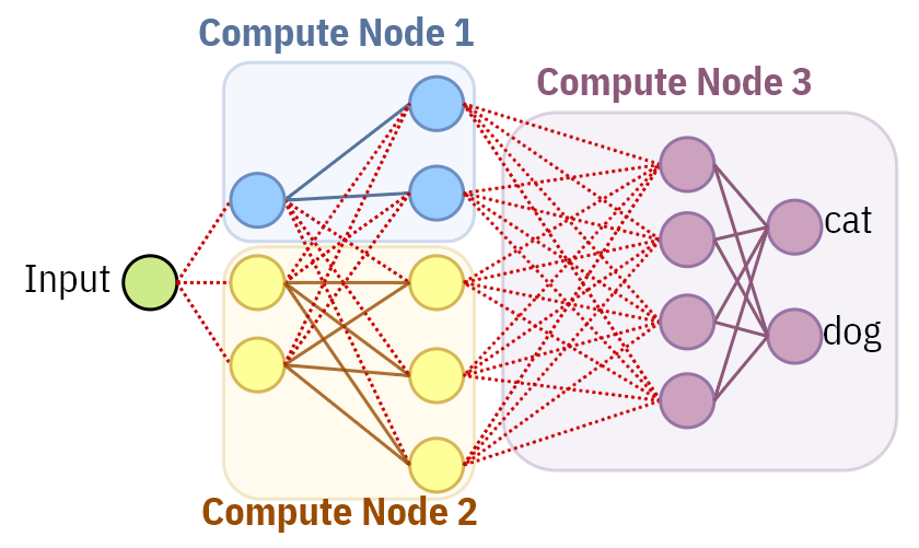
(a) Model Parallelism

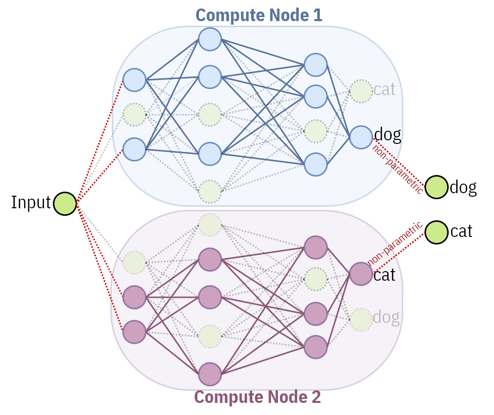
(b) Class Parallelism

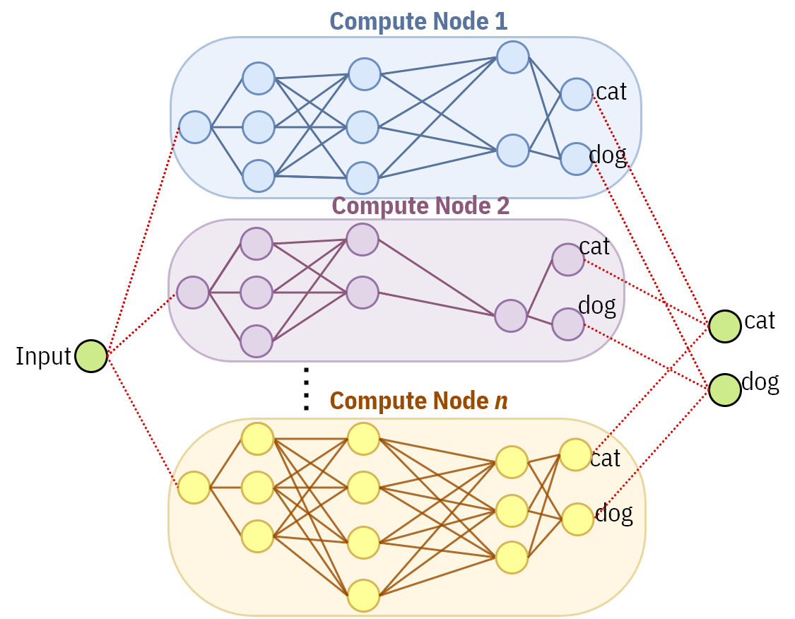
(c) Variant Parallelism

Figure 1: Comparison of different model distribution methods on atomic input data. In (b), some neurons and connections (opaqued in the picture) are pruned so that each model predicts only one class to improve overall performance.

For atomic data that cannot be split into further pieces [6], two major solutions are often used to decompose and distribute a model accross compute resources; namely, model parallelism (MP) and class parallelism (CP). MP decomposes a model into multiple sequential or parallel slices, each sent over to a separate compute node for processing, then lots of intermediate data values are returned to the master to combine and complete the model. Slicing in MP can be inter- or intra-layer (Fig. 1a). CP decomposes the model into multiple disjoint models, each aiming to predict only one or a few non-overlapping classes (Fig. 1b); thus, contrary to MP, CP runs a monolithic model on each computing node. CP improves efficiency of each model mostly by applying class-aware pruning policies [6].

Both solutions have their own limitations. In MP, intermediate tensors have to be communicated between different nodes. In current CNNs, the time needed to transmit intermediate tensors can be orders of magnitude higher than inference time itself. Hence, MP would drastically increase end-to-end latency [7]. CP does not suffer from this issue since there is no sequential dependency and each computing node only returns a few numbers; these numbers represent the prediction of classes allocated to the submodel executed on that node. Verbatim CP has a firm restriction on scalability that is limited to the number of classes in the application [6], which can debatably be extended by choosing overlapping subsets of classes instead. However more importantly, both paradigms intrinsically suffer from multiple instances of single point of failure (SPOF) issue because every compute node has to complete its job and send the result back to the requesting node before the top-level classification task can be fully finished. Otherwise, the master node cannot generate the final network prediction. Therefore, failure in a single node compromises availability of the whole system. The scenario of interest in this paper is where we use the free times of IoT devices to do a distributed inference job. Failure is a common problem in distributed systems, especially in this scenario of cycle-stealing from nearby IoT devices, where worker nodes only contribute in idle times and at any times may preempt the inference task to process their main jobs [8], and some nodes may seriously slow down due to various unexpected reasons. Additionally, communication issues such as network congestion, lead to missed deadlines in real-time applications. These concerns motivate the need for a fault-tolerant mechanism. Obviously, in both MP and CP, higher availability may be achieved by introducing redundant nodes, but of course this comes at the expense of large impact on communication and computation cost.

In this paper, we propose a distribution technique: Variant Parallelism (VP). Both MP and CP can be viewed as applying a “top-down” model slicing approach: they try to break a baseline model into pieces, although differently in MP vs CP, and distribute each piece across multiple nodes. In contrast, we in VP employ a “bottom-up” approach: we generate multiple variants (described below) from a chosen basic architecture and then combine their results in an aggregator component (Fig. 1c). In fact, CP and VP are both special types of ensemble learning models, but with different intents and approaches.

In VP, each variant is an independent model that can be deployed on a different machine or accelerator. Unlike CP, our variants have full-class prediction heads, i.e., each worker node predicts probabilities for all classes, and this is the key in achieving a fault-tolerant architecture. Consequently, in a system with $n$ worker nodes, VP can still get a full response even if $n\mathchar 45\relax 1$ nodes fail, while having the variants helps to improve accuracy over naïve replication when more than one worker node is working. VP’s variants can differ in input resolution and input offset. To achieve faster inference time, we apply three network optimizations: narrowing network width, reducing complexity of the compute intensive layers, and replacing with faster operations when possible.

Since each machine generates full-class prediction, the data transmission amount would be higher than CP, resulting in risking a higher response time. To avoid this, we put a compression/decompression module. The compression layer attaches to each worker’s classification head. In the compression part we select $k$ classes with the highest confidence score and send them to the master together with their corresponding indices. In VP, each machine executes a lightweight classification model, and sends its compressed result to the master. The master machine then applies a decompression step followed by a score scaling to weight each prediction based on its corresponding model capacity. It eventually combines results via an aggregation module. There is no trainable parameter in the combination modules. Otherwise, it reduces system’s flexibility and can compromise availability. For evaluation, we consider a smart home scenario and demonstrate VP’s robustness on seven object recognition benchmarks.

Our major contributions can be summarized as follows:

• We introduce a bottom-up model distribution called Variant Parallelism which contrary to MP and CP is fault-tolerant, flexible, and therefore, can be freely distributed across several sporadically available compute nodes such as the case of IoT devices or across multiple accelerators within a single machine.

• Our technique generates multiple variants each having different number of parameters, multiply-accumulate operations (MACs), latency, and model size that can be deployed on different machines based on their capacity.

• We propose an aggregation method that is resilient to failures, while matching accuracy of the baseline.

• We propose a fast and simple technique to reduce bandwidth usage. It can compress the output size of each node by up to $10\times$ while losing less than $0.5\%$ accuracy. The gain would be two orders of magnitude higher on benchmarks with large number of classes, e.g., ImageNet.

• Our proposed method can have $5.8\mathchar 45\relax 7.1\times$ fewer parameters, ${4.3\mathchar 45\relax 31\times}$ fewer MACs, and ${2.5\mathchar 45\relax 13.2\times}$ lower response time on an atomic input compared to the baseline while achieving comparable or higher accuracy.

II Related Work

Model Parallelism (MP): In model parallelism (Fig. 1a) a deep learning model is sliced into multiple sub-models [9, 10]. Each of them can be deployed and concurrently and/or sequentially executed on multiple machines. These sub-models have to transfer data from intermediate tensors. The time to transfer these tensors can be orders of magnitude higher than the time to compute operations of the neural network itself. For example, [7] shows that the intermediate outputs of deep learning models are $19$-$4500{\times}$ larger than the compressed input. Recent proposals’ focus has mostly been on reducing communication rounds [11] or its overhead [12]. Though, the SPOF problem is still inevitable and inherent to MP.

Class Parallelism (CP): It decouples a base model into multiple independent sub-models, each can predict one or a few non-overlapping classes (Fig. 1b). Structured pruning is then applied on each sub-model to reduce their latency. The ultimate result can be prepared by combining the prediction of all of these sub-models [6, 13]. CP does not have the issue mentioned for MP, and can improve latency compared to a single model. However, it has a hard limitation on the number of sub-models. More importantly, both MP and CP require results from all machines and suffer from mutiple SPOFs.

Variant parallelism (VP) works on atomic live data and by design tolerates up to $n\mathchar 45\relax 1$ nodes failure. Contrary to other techniques, VP gives us the flexibility to generate enough variants based on different objectives including latency constraints, model size (proportional to the number of parameters), and compute resources. VP can be easily combined with other parallelism schemes.

III Variant Parallelism

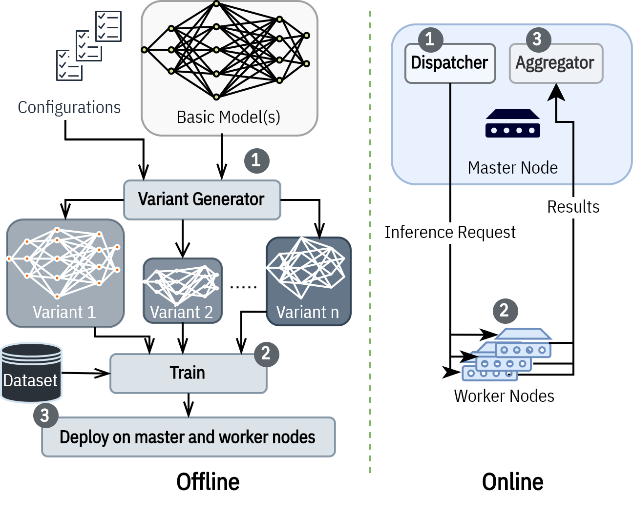
Figure 2: Overview of our proposed workflow including offline parts (variant generation and model training) and online actions (dispatcher and aggregator).

In VP, we consider a basic model, and generate multiple lightweight and fast models based on it. Each of these variants can have different storage sizes, parameters, inference times, and accuracies. We add inference-time augmentation, that leads to feeding slightly different inputs for each model. Each variant can be treated as an independent full-class predictor: Every machine can concurrently execute one or more of these variants in-parallel with other machines. Depending on the use-case, these machines may be different GPUs on a single node or different edge devices, which is the case of interest in this paper. If there is an idle node with limited storage space or computation constraints, VP can generate a lighter variant which provides the opportunity to utilize the available compute capacity. VP aims to reduce response time to enable faster decision making via a distributed deep learning architecture while maintaining availability in presence of failure.

III-A Overview

Our workflow starts with one basic architecture, but is straightforward to extend to more than one model. As shown in Fig. 2, we generate different variants from the base model(s). We then add classification head, compression, decompression, and scaling modules to each variant. Variants are retrained on the desired dataset. These variants are independent and can be separately deployed on different machines for distributed in-parallel execution. Every node has its own model. Once deployed, the master node multicasts live data to all contributing workers, and waits for a predefined period (proportional to the desired deadline). The workers feed the data into their models and send the compressed result back to the master node. The master then decompresses, scales and combines them through the aggregation module to prepare the final prediction (Fig. 3).

III-B Reducing Model Complexity

For variant generation, we reduce complexity of the basic architecture through the following three steps: (1) reducing width factor, (2) reducing complexity of the last few layers, and (3) replacement with faster operations when possible. These steps help us to improve per machine model size, computation requirements, and latency. Firstly, we reduce width factor of depth-wise separable convolution layers (was first introduced in [14]) by $2.85{\times}$ ($2{\times}$ for ImageNet variants). It improves network runtime [14]. We recover the lost accuracy by combining multiple parallel variants (§ IV-E). Secondly, we reduce complexity of the last few layers of each variant based on its input size. The intuition is that in the current efficient CNNs, the last few layers take considerable portion of the computation time. However, it should be proportional to the input resolution and the achievable accuracy. As shown in Table I, each model uses convolutional layers with the number of filters ($f$) proportional to its input size ($\rho_{i}$). For example, input size of $V_{3}$ ($i{=}3$) is $160$ and its last convolution layer has $384$ output filters while $V_{1}$ ($i{=}1$) with input size of $96$ has only $256$ output filters. We empirically select the number of these output filters so that they are divisible by $64$ for better performance. In that sense, the first and second steps are types of structured pruning that result in fewer parameters and MACs. Lastly, we employ faster operations when possible, e.g., replacing $FullyConnected$, $AveragePooling$, and $Average$ layers by $1\times 1Convolution$, $MaxPooling$, and $Add$ layers, respectively. We generate five (for CIFAR-10, CIFAR-100, MNIST, F-MNIST and SVHN) and seven (for ImageNet and Food101) different models based on these optimizations. Their characteristics are illustrated in Table II.

TABLE I: Variants model architecture.

Input	Operator	$t$	$f$	$n$
$3\times\rho_{i}^{2}$	conv2d	-	32	1
$32\times\rho_{i}^{2}/4$	bottleneck	1	16	1
$16\times\rho_{i}^{2}/4$	bottleneck	6	24	2
$24\times\rho_{i}^{2}/8$	bottleneck	6	32	3
$32\times\rho_{i}^{2}/16$	bottleneck	6	64	4
$64\times\rho_{i}^{2}/32$	bottleneck	6	96	3
$96\times\rho_{i}^{2}/32$	bottleneck	6	160	3
$160\times\rho_{i}^{2}/64$	bottleneck	6	320	1
$320\times\rho_{i}^{2}/64$	conv2d $1\times 1$	-	${64{\times}j}$	1
$(64\times j)\times\rho_{i}^{2}/64$	globalmaxpool	-	-	1
$(64\times j)$	conv2d $1\times 1$	-	$C$	-
$C$	compression	-	$k$	-

Similar to the original MobileNetV2, we apply a convolution layer on input followed by $19$ depth-wise convolutional residual bottlenecks. Each row is sequentially applied $n$ times, and $t$ is the expansion factor of intermediate layers in bottleneck blocks. $C$ is the number of classes. $j{=}(3+i)$ when width-factor=0.35 and $j{=}\min\left[(7+2i),20\right]$ when width-factor=0.5 (for ImageNet variants).

TABLE II: Comparison of different models’ characteristics

Model	Input Size	#Params	#MACs
MobileNetV2	$3\times 224^{2}$	2.27M (3.47 on ImageNet)	300M
$V_{7}$	$3\times 320^{2}$	410K	112M
$V_{6}$	$3\times 256^{2}$	390k	71M
$V_{5}$	$3\times 224^{2}$	370K	54M
$V_{4}$	$3\times 192^{2}$	360K	40M
$V_{3}$	$3\times 160^{2}$	340K	27M
$V_{2}$	$3\times 128^{2}$	330K	17M
$V_{1}$	$3\times 96^{2}$	320K	10M
$V_{im7}$	$3\times 320^{2}$	1.97M	196M
$V_{im6}$	$3\times 256^{2}$	1.9M	125M
$V_{im5}$	$3\times 224^{2}$	1.75M	95M
$V_{im4}$	$3\times 192^{2}$	1.59M	69M
$V_{im3}$	$3\times 160^{2}$	1.45M	47M
$V_{im2}$	$3\times 128^{2}$	1.3M	30M
$V_{im1}$	$3\times 96^{2}$	1.15M	17M

Variants $V_{im[i]}$ are exclusively designed for ImageNet benchmark [15].

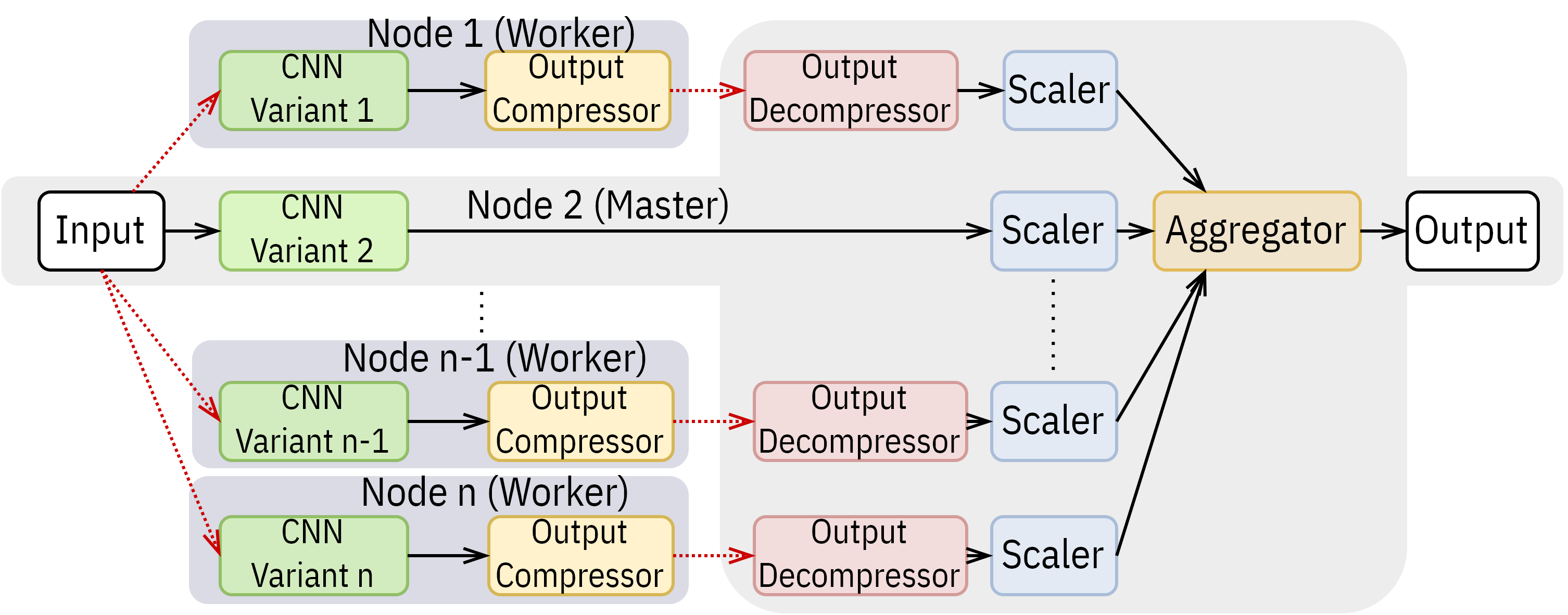
Figure 3: The flow of data and the online operations on them, for inference.

III-C Compression and Decompression

In CP, for tasks with only few classes (e.g., CIFAR-10), each machine returns only one floating point, and for tasks with more classes (e.g., CIFAR-100), 10 to 20 floating point values are returned by each. In contrast, our variants are independent models that can return full-class prediction. This feature increases the system reliability in a faulty environment, but raises a challenge in communication time. To address the mentioned issue, we leverage the $Top\mathchar 45\relax k$ idea in which from a prediction vector $\psi_{i}$, we select $k$ elements having the highest confidence scores and pack them along with their corresponding indices. Fig. 4 depicts a toy example with 6 classes, assuming $k=2$. The compression step shrinks the vector size to two vectors of size $k$: One stores floating point predictions with the highest score ($0.51$ and $0.4$), and the second keeps their integer indices ($1$ and $3$). After receiving compressed vectors, the master reconstructs a tensor of shape ($batch\_size,V,C$), where $V$ and $C$ are the number of total contributing machines and classes, respectively. It then scatters values of compressed vectors based on their indices. This procedure is fast yet robust. The intuition behind is that in each vector except a few elements with high confidence scores, others are close to zero. More importantly, our aggregation method (§ III-D) amplifies both actual information and noise at the same time. Hence, by removing values with lower confidence score, we actually mitigate noisy information to some degrees, and consequently achieve higher accuracy.

III-D Scaling and Aggregation

Master is responsible for balancing the prediction vectors of different variants. After decompression step, we apply a $Softmax$ operation to transform the reconstructed prediction vectors into a probability distribution (Fig. 4). We then need to scale each prediction vector based on its network capacity. For example, if variant $V_{i}$ has more parameters, and thereby returns more accurate predictions than variant $V_{j}$, then it deserves to have a higher weight in the aggregated result. We use a proxy of the network architecture itself to scale values of every prediction vector via eq. 1.

$$\psi_{i}=(\frac{\rho_{i}}{\max(P)})(\frac{d_{i}}{\min(D)})^{\alpha}.\psi_{i}$$ (1)

$$where~{}~{}\rho_{i}\in P~{}~{},and~{}~{}d_{i}\in D$$ (2)

Where $\psi_{i}$ is the prediction vector of variant $V_{i}$ with input shape $\rho_{i}$ and depth multiplier $d_{i}$, and $\alpha$ is a parameter to equalize the impact of input shapes and depth multiplier.

In the aggregation module we combine prediction results that are received from compute nodes including the master itself. We add the vectors together and apply a $Softmax$ afterwards. Using FullyConnected ($fc$) layers instead, although might improve accuracy, degrades flexibility. Furthermore, with the same number of neurons as the number of classes $C$, and $V$ variants contributing in the aggregation step, the computation cost of using only a single $fc$ layer would be $O(CV)$ which is $O(V)$ times higher.

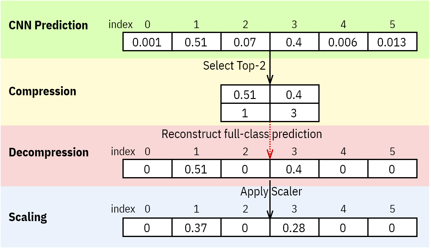
Figure 4: An example of compression, decompression and scaling steps assuming $C=6$ and $k~{}(in\>Top\mathchar 45\relax k)=2$.

IV Experiments

IV-A Experimental Setup

Compute Platform: We use an in-house server (Table III), to design, train and evaluate our models. We selected the commonly reported vision datasets that are trainable on our server in a reasonable time.

TABLE III: Server specification

CPU	Intel Xeon E5-2630-v3 (x86_64)
	Frequency: 2.4GHz (1.2-3.2GHz)
GPU	NVidia GeForce GTX 1080 Ti
	Total Memory: 11GB
Memory	32GB (1600MHz)

Benchmarks: We have provided six different mid-sized object recognition datasets that can be categorized into three complexity levels (in terms of the achievable accuracy by the baseline architecture): simple (CIFAR-10 [16], Fashion MNIST (F-MNIST) [17], Fashion MNIST (F-MNIST) [17], MNIST [18] and SVHN [19]), mediocre (CIFAR-100 [16]) and difficult (Food-101 [20]). For completeness, we additionally provide accuracy results on ImageNet-1k (i.e., 1k classes) [15].

TABLE IV: Datasets used for evaluation

Dataset	$C$	Input Size	#Trains	#Tests
Food-101	101	$3\times 256^{2}$	75,750	25,250
SVHN	10	$3\times 32^{2}$	73,257	26,032
CIFAR-10	10	$3\times 32^{2}$	50k	10k
CIFAR-100	100	$3\times 32^{2}$	50k	10k
MNIST	10	$28^{2}$	60k	10k
F-MNIST	10	$28^{2}$	60k	10k
ImageNet	1000	$3\times 256^{2}$	1.28M	50k

Edge Device: For latency evaluation of different models, we use a mid-range tablet (Table V), and leverage Google TFLite native benchmark tool [21] to profile the performance.

Baseline Model: We consider MobileNetV2 [4] as our basic architecture (Table II). It is regarded as an efficient model designed for constrained edge devices. Thus, if we show gains in comparison to MobileNetV2, as we did, then one can expect similar results on models with more redundancy.

IV-B Training

We trained $V_{1}$ through $V_{7}$ for $135$ epochs. Our training procedure has two steps. For the first 30 epochs, all layers except the last two convolutions were frozen. For the ImageNet variants ($V_{im[i]}$), we iterate 75 epochs (the first 40 for fine-tuning). We port pre-trained weights from ImageNet-1k [15] whenever available. We used batch size of 128 in this step, and 64 (32 in Food-101) for the rest of 105 epochs. We used Adam optimizer with $\beta_{1}=0.9$ and $\beta_{2}=0.999$. Learning rate decays by a factor of $0.98$ once the accuracy stagnates. We do not apply hyperparameter optimization. Thus, one may improve the results by doing so. Since our tasks are classification, and each model can independently predict all of the classes, we apply a separate categorical cross entropy for each model. Contrary to CP, our variants can observe the same data during training. Therefore, we train multiple models along with the combination components all together. The number of models that can be trained simultaneously is a parameter that can be set based on the computation capacity. Having more models requires more memory, but improves GPU utilization as most parts of our data pipeline executes once. To avoid overfitting, we apply typicaly used augmentation methods namely random horizontal flip, random rotation and MixUp.

IV-C Accuracy of Single Models

First, we evaluate accuracy of each variant and compare it to the accuracy of our baseline. To have a fair comparison, we trained the baseline with the same training policy, and made sure it has the same or higher accuracy compared with original reports, if applicable. For each dataset, we report the accuracy of five (seven for Food-101 and ImageNet) different models. We also report $top\mathchar 45\relax 2$ and $top\mathchar 45\relax 5$ in aggregator for datasets with ${C<100}$ and ${C>=100}$, respectively. Here, by $top\mathchar 45\relax m$ we mean the ground-truth label is among top $m$ class predictions with the highest confidence scores. As depicted in Table VI, as we go from the variant $V_{1}$ to $V_{7}$ ($V_{im1}$ to $V_{i}m7$ on ImageNet), the accuracy improves. For the datasets with few number of classes, the accuracy of $V_{5}$ is close to the baseline. Nevertheless, our $V_{5}$ has ${\sim}6\times$ fewer parameters and MACs. This shows that for simple tasks with few classes, we can already reach to the baseline accuracy level without the need for parallelism. In fact, our bottom-up ensemble design gives us the flexibility to pick only one or a few variants for a custom use-case scenario while in model and class parallelism, all models are mandatory. Yet, by using variant parallelism, as we explain next, we can achieve even higher accuracy levels compared with the baseline.

TABLE V: Edge device specification

Samsung Galaxy Tab A 8.0 with S Pen (2019, SM-P205)
CPU	Octa-core big.LITTLE (2x1.8 GHz Cortex-A73 and 6x1.6 GHz Cortex-A53)
GPU	ARM Mali-G71 MP2
Memory	3GB LPDDR4X
Network	Wi-Fi 802.11, estimation: RTT=2ms bw=1Mbps

TABLE VI: Accuracy (%) of single models on different datasets

Dataset	Metric	MobileNetV2	$V_{1}$	$V_{2}$	$V_{3}$	$V_{4}$	$V_{5}$	$V_{6}$	$V_{7}$
CIFAR-10	Top-1	95.16	91.76	93.07	93.81	94.43	94.62	-	-
	Top-5	98.57	97.24	97.87	98.20	98.26	98.29	-	-
MNIST	Top-1	99.37	99.38	99.41	99.41	99.42	99.46	-	-
	Top-2	99.87	99.92	99.95	99.89	99.92	99.95	-	-
CIFAR-100	Top-1	80.51	69.62	73.57	74.46	74.67	75.20	-	-
	Top-5	94.9	91.17	93.36	93.47	93.41	93.67	-	-
SVHN	Top-1	95.52	93.81	95.16	95.34	95.89	95.91	-	-
	Top-2	98.37	97.47	98.21	98.25	98.46	98.32	-	-
Fashion-MNIST	Top-1	94.41	93.38	94.16	94.60	94.67	94.55	-	-
	Top-2	98.82	98.30	98.51	98.76	98.84	98.82	-	-
Food-101	Top-1	79.68	58.78	65.35	70.13	71.43	74.23	74.64	75.79
	Top-5	93.5	83.50	87.70	90.19	90.78	92.43	92.52	93.15
Dataset	Metric	MobileNetV2	$V_{im1}$	$V_{im2}$	$V_{im3}$	$V_{im4}$	$V_{im5}$	$V_{im6}$	$V_{im7}$
ImageNet	Top-1	67.5	48.8	54.7	57.9	61	62.25	63.2	64.9
	Top-5	87.9	73.65	78.7	80.9	83.3	84.2	85	86

IV-D Impact of Compression Method

In this section, we analyze the effect of our compression algorithm on accuracy and the required bandwidth. We feed the same input data to all variants, and evaluate the impact of different values for $k$ in our compression module.

Bandwidth Saving: Output size is a linear function of $k$.

$$h(k)=\begin{cases}\min\{k\times[\text{size}(fp)+1],\text{size}(fp)\times C\}&k>1\\ 1&k=1\end{cases}$$ (3)

Where $h(k)$ is the output size in byte, $\text{size}(fp)$ is the number of bytes required for storing a floating point value and $C$ is the number of classes. Among different $k$ values, $k=1$ is a special case. Because the compressor selects only one element, we can further reduce communication cost, sending only an integer representing its index. It can be found that choosing $k>\frac{C}{2}$ is not logical as transmitting the whole vector actually costs less than compressing it.

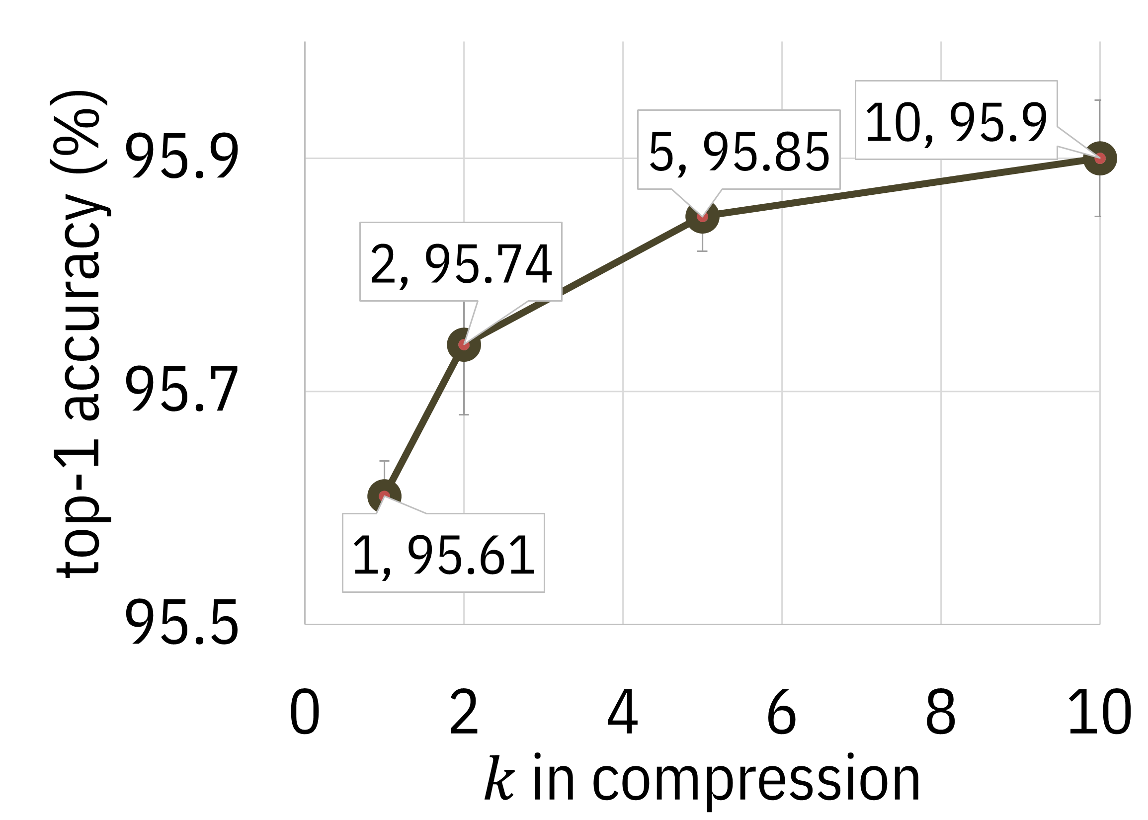
(a) CIFAR-10 aggregator Top-1

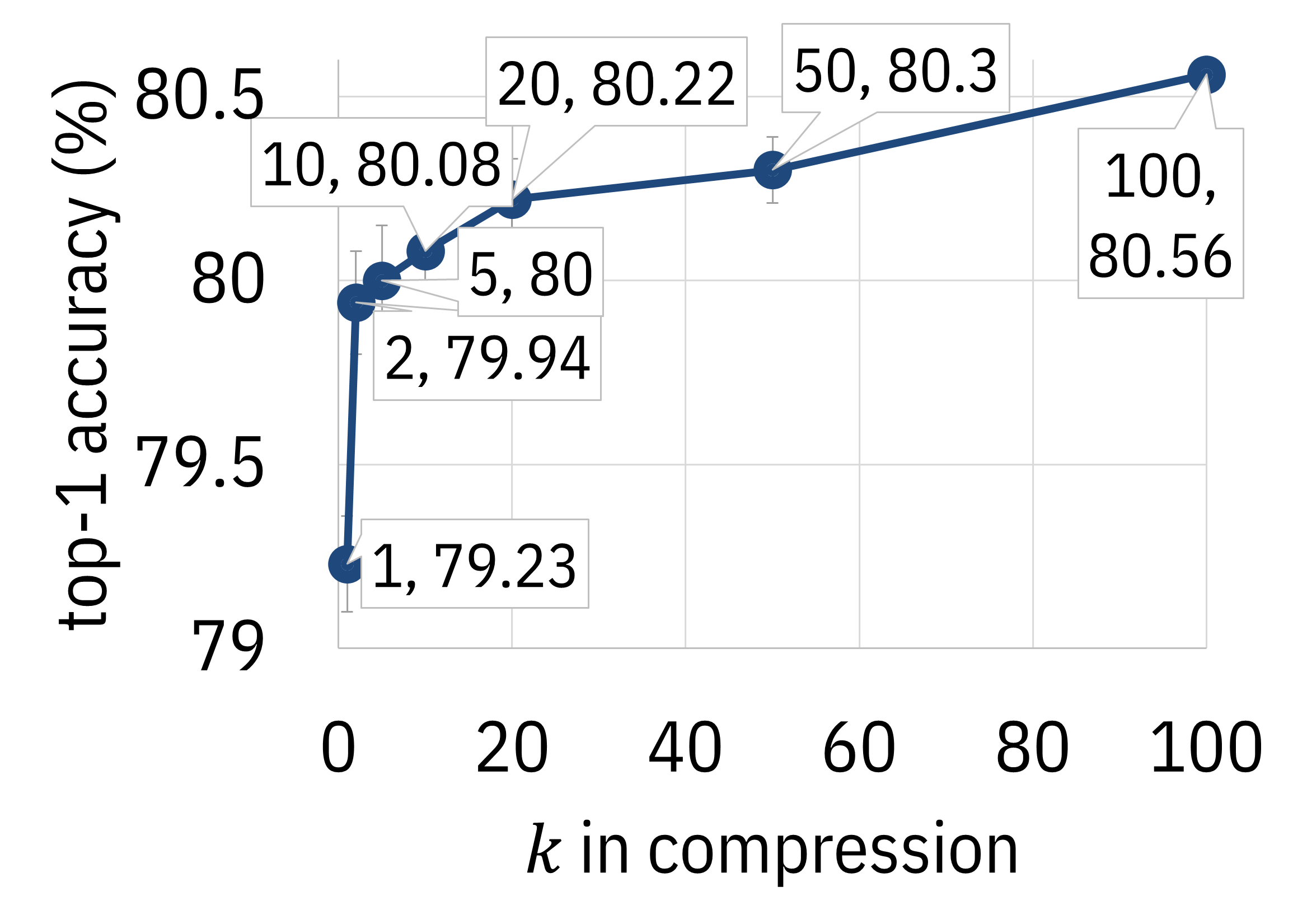
(b) CIFAR-100 aggregator Top-1

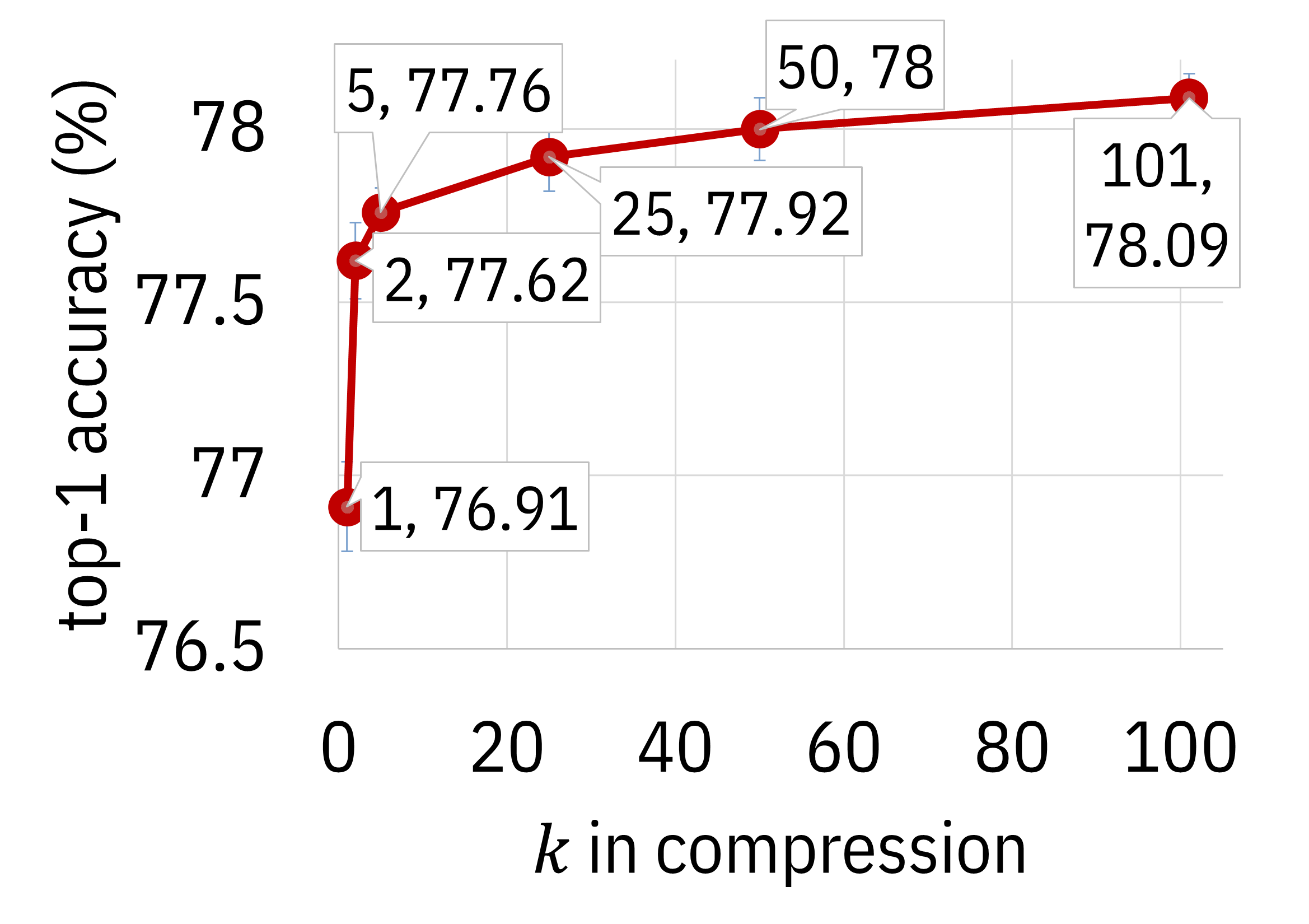
(c) Food-101 aggregator Top-1

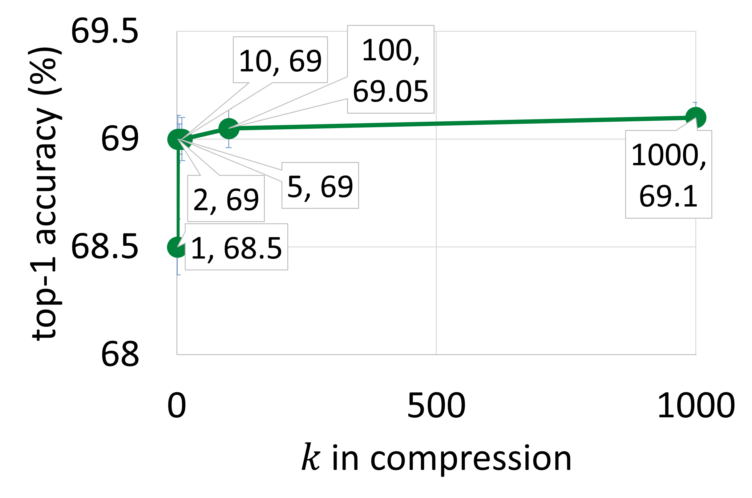
(d) ImageNet aggregator Top-1

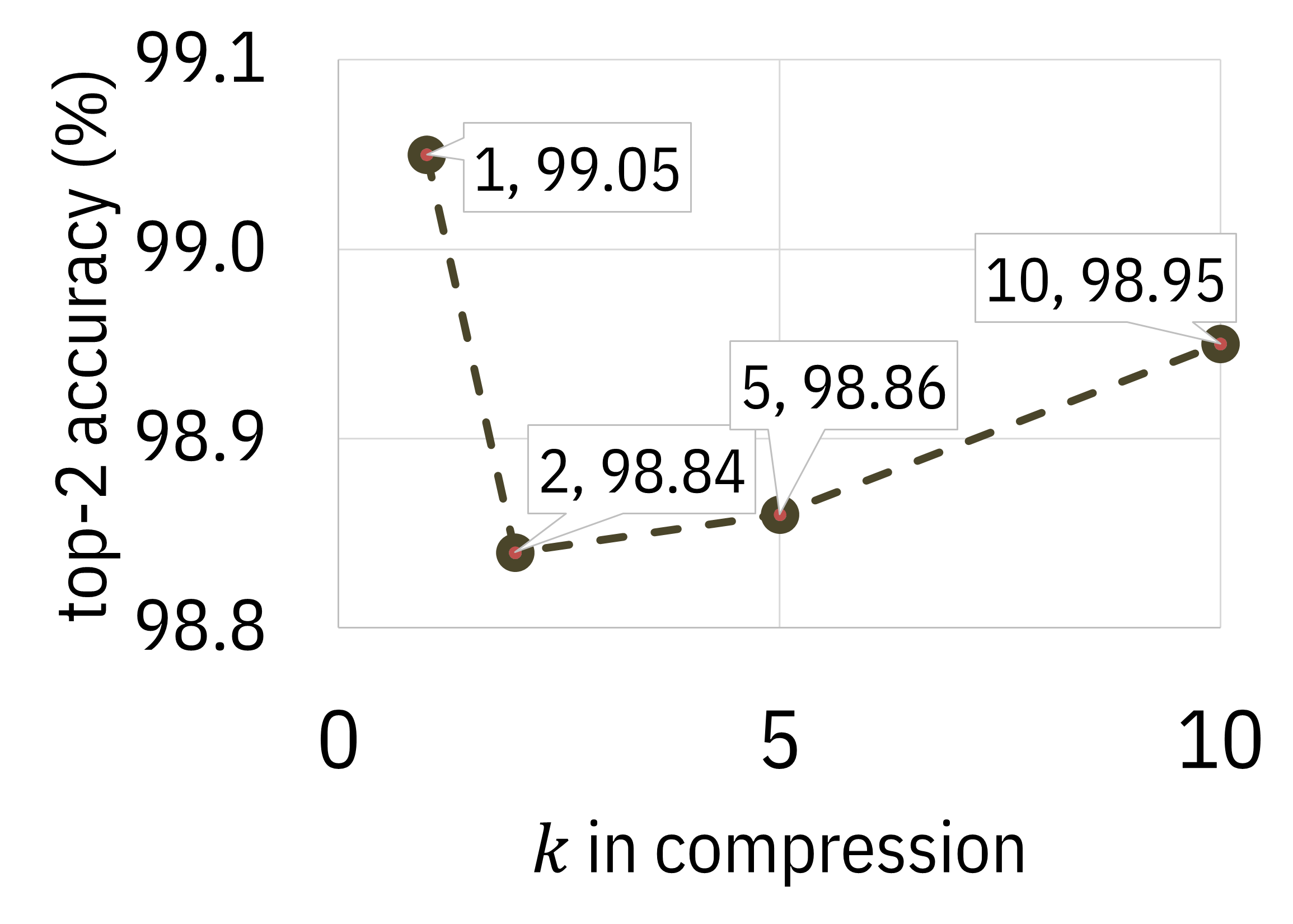
(e) CIFAR-10 aggregator Top-2

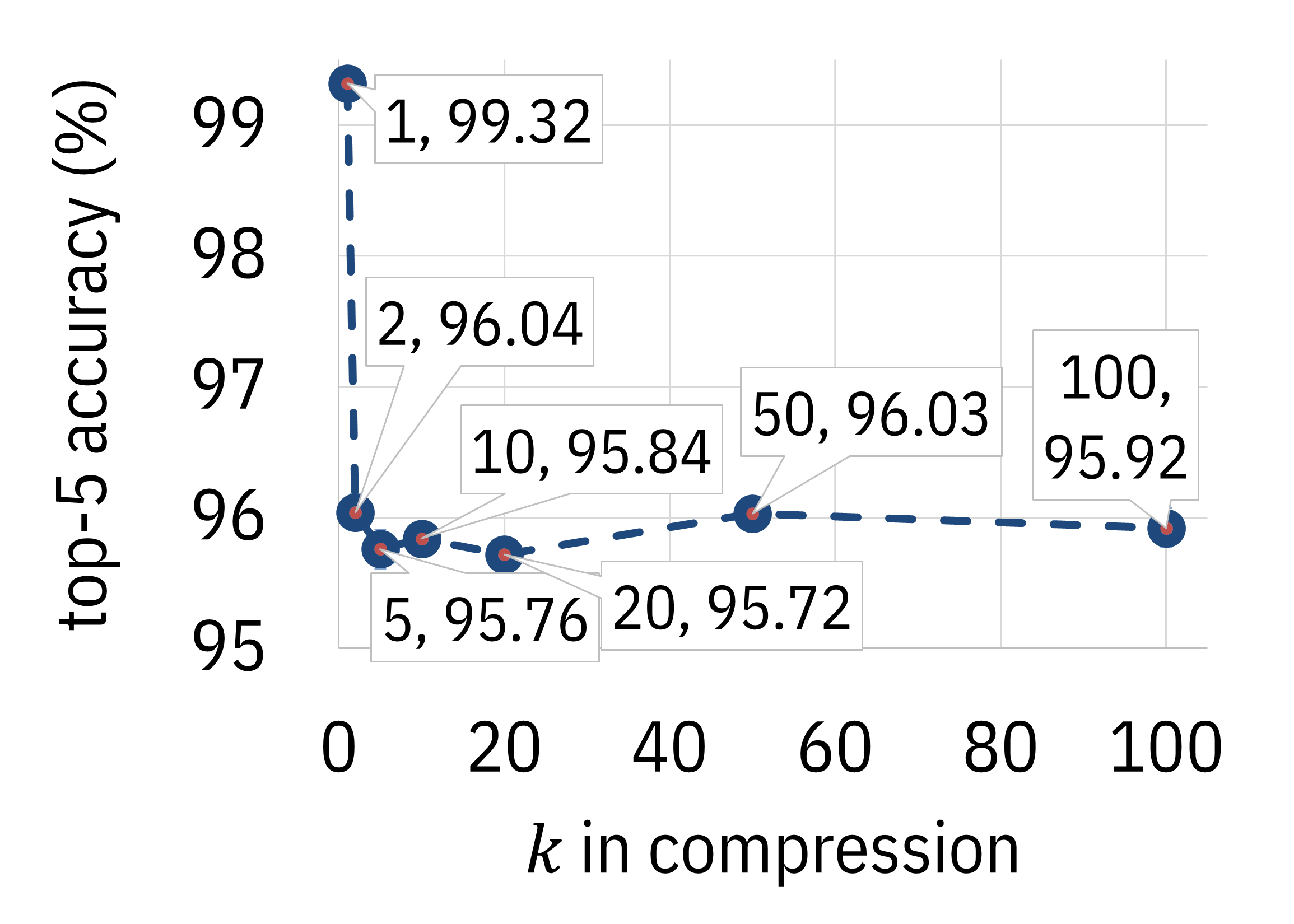
(f) CIFAR-100 aggregator Top-5

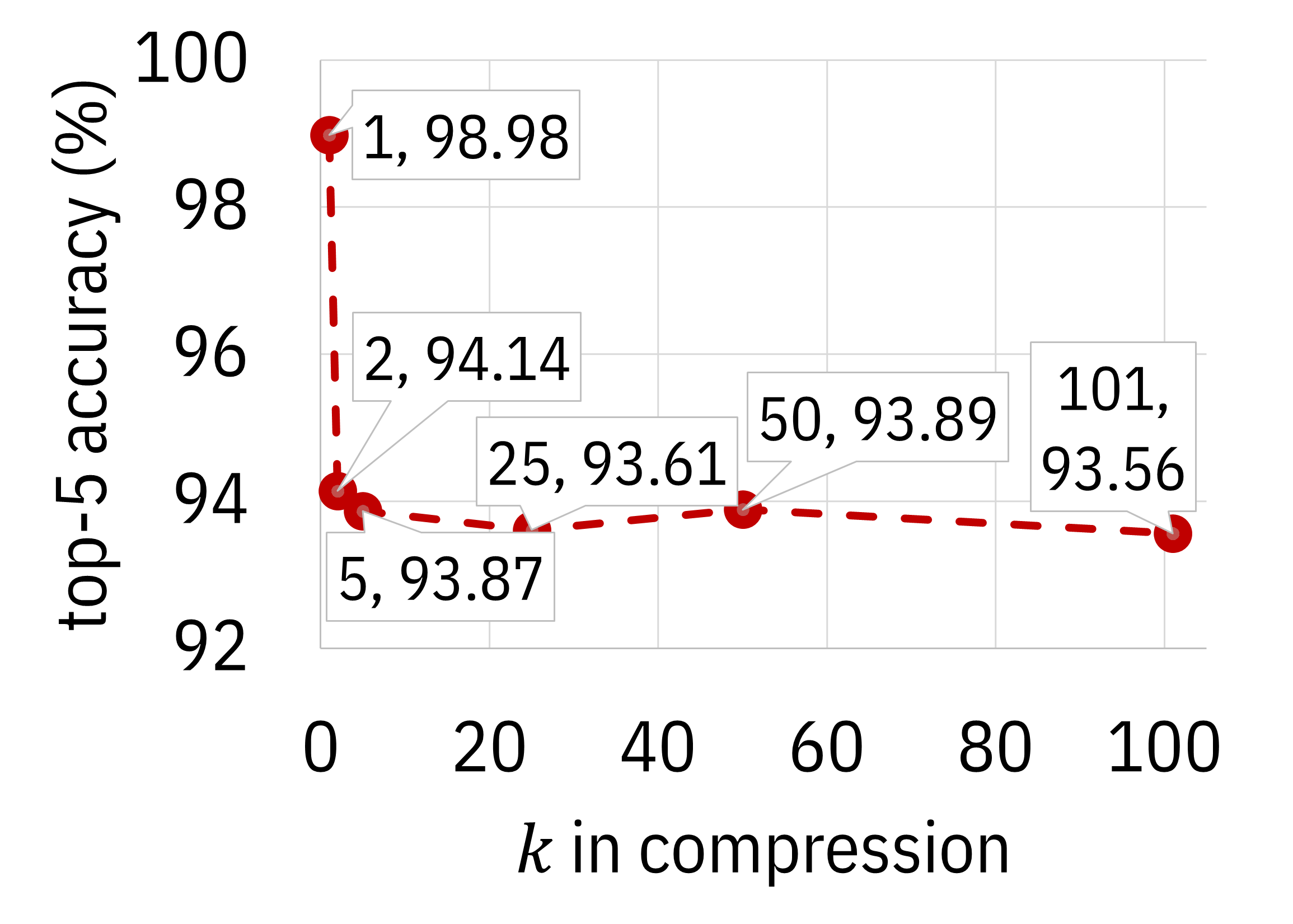
(g) Food-101 aggregator Top-5

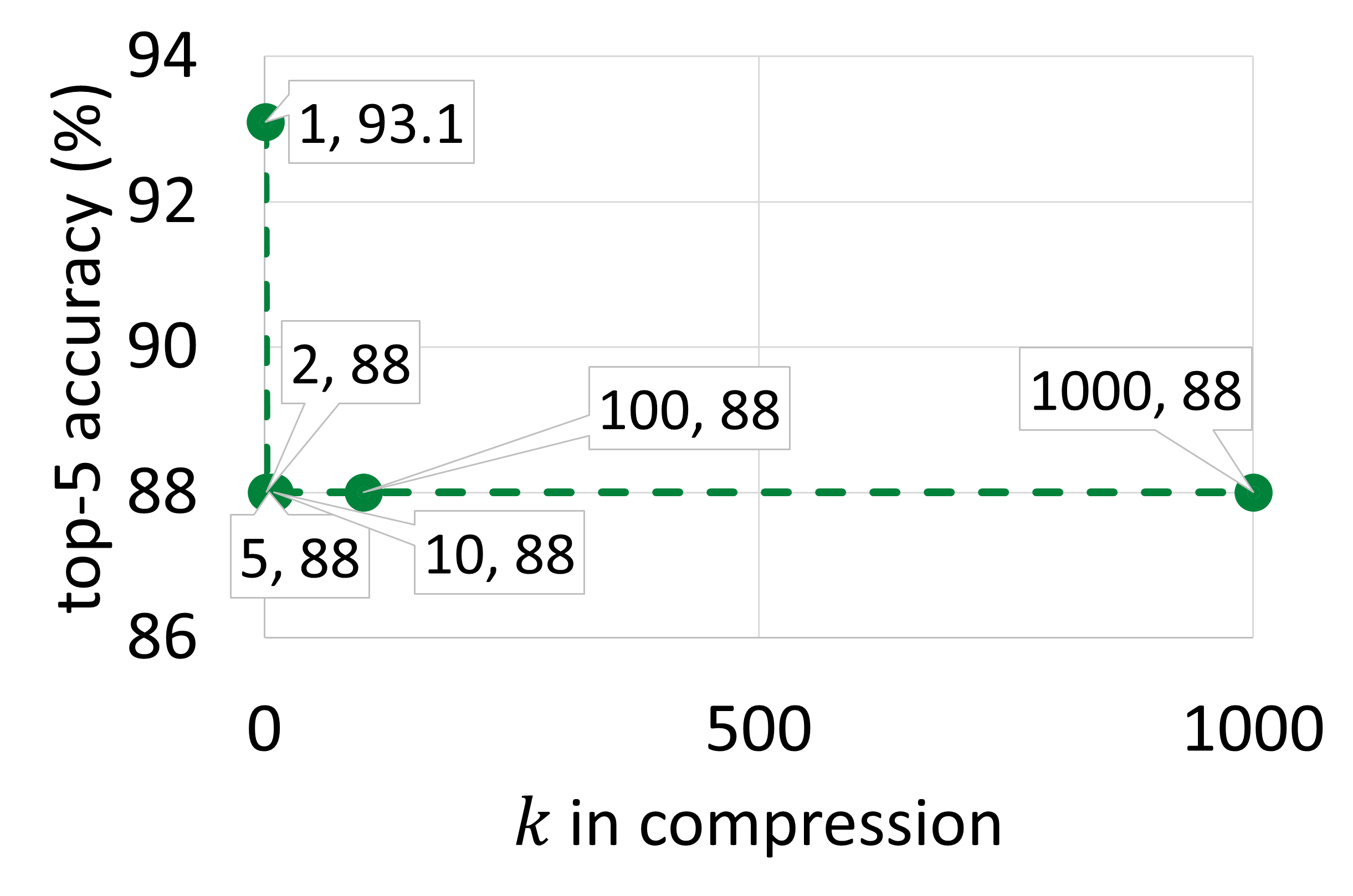
(h) ImageNet aggregator Top-5

Figure 5: Impact of different $k$ values on accuracy of different benchmarks. $k$: the number of top predictions returned by each node.

Ensemble Accuracy: In this experiment, we evaluate how different values of $k$ can impact the final accuracy. Fig. 5 illustrates a significant jump in $top\mathchar 45\relax 1$ accuracy from $k=1$ to $k=2$. For $k>2$, the accuracy does not significantly increase. Another interesting observation is on $top\mathchar 45\relax m$ accuracy: sending the prediction with the highest confidence score per variant improves $top\mathchar 45\relax m$ accuracy. The reason is that when aggregating multiple prediction vectors, classes with lower scores behave like noise. By omitting these elements from our prediction vectors, we indeed achieve higher $top\mathchar 45\relax m$ accuracy. It appears to be a trade-off between higher $top\mathchar 45\relax 1$ and $top\mathchar 45\relax m$ accuracies. Apparently, $k=2$ is a good choice and we use it for the rest of our experiments.

IV-E Scaling Accuracy

We generated different variants each having unique characteristics. Here, we analyze the impact of combining different variants on the ensemble accuracy (Fig. 7). We show results on CIFAR-10, CIFAR-100, Food-101, and ImageNet. The other three datasets behave similarly to CIFAR-10. We show the final combined accuracy with respect to the average per-device MACs. Note that the horizontal axis is the average MACs over participating variants. We also added results from the combination of the variants $V_{1}$ through $V_{5}$ ($V_{7}$ on Food-101 and ImageNet) while using ${k=5}$ (in the compression module) and without compression as well. To clarify, $V_{i}$ on the figures belonging to the results on ImageNet refers to $V_{im[i]}$. It is worth noting that even the combined number of parameters and MACs of our models are fewer than the baseline, except the ImageNet variants which are still less complex than the baseline. On CIFAR-10, we almost reach the same accuracy as the baseline by combining $V_{1}$, $V_{2}$, and $V_{3}$. Addition of $V_{4}$ and $V_{5}$ improves the accuracy incrementally and enables us to achieve even better results than the baseline. On CIFAR-100, comparable accuracy can be achieved by aggregating the results of all five variants. The most MACs is required by $V_{5}$ which is ${\sim}6\times$ fewer than the original MobileNetV2. The Food-101 dataset is rather more complex as the size of its original images are two orders of magnitude bigger than the other benchmarks. To achieve comparable results, we generated $V_{6}$ and $V_{7}$. We reach similar accuracy to the baseline by combining the first six variants. Inclusion of $V_{7}$ further improves the result, however, at the cost of more computation. The ImageNet dataset is far bigger than the other benchmarks both in input size and number of classes. Therefore, the variants uesd so far ($V_{1}$-$V_{7}$) do not provide reasonable accuracy. Consequently, we designed, generated and report seven new and more capable variants ($V_{im1}$-$V_{im7}$). These new variants differ in depth multiplier ($d_{i}{=}0.5$) and the number of neurons in the last layer, and therefore are larger and more accurate than the previous ones (see Table II). Similar to Food-101, we achieve an accuracy comparable to the baseline via ensemble of the first six variants. Addition of $V_{im7}$, leads to further improvement.

In all the benchmarks, increasing $k$ in the compression step or transmitting the predictions without any compression gives better results but the differences are not significant. Intrestingly, by increasing the number of variants to ${>=}6$ in the Food-101, this gap disappears. This can be due to the increase in the number of variants, particularly one or two more accurate ones.

IV-F Effect of Every Variant on Accuracy

To find out whether each variant actually impacts the final accuracy, we evaluate the predictions returned by the combination of our variants while excluding only one of them. As shown in Fig. 7, in all datasets, omitting each variant has a negative impact on the final accuracy. This is especially interesting in less accurate variants. For example, on CIFAR-100, $V_{1}$ has ${\sim}70\%$ accuracy itself which is more than $10\%$ lower than the baseline, yet when included in the aggregation, it can improve the final accuracy. Same is true in the other benchmarks except. On ImageNet, however, we do not observe this pattern. Interestingly, although addition of variants increases accuracy (Fig. 6d), excluding one of them does not seem to negatively impact the final accuracy.

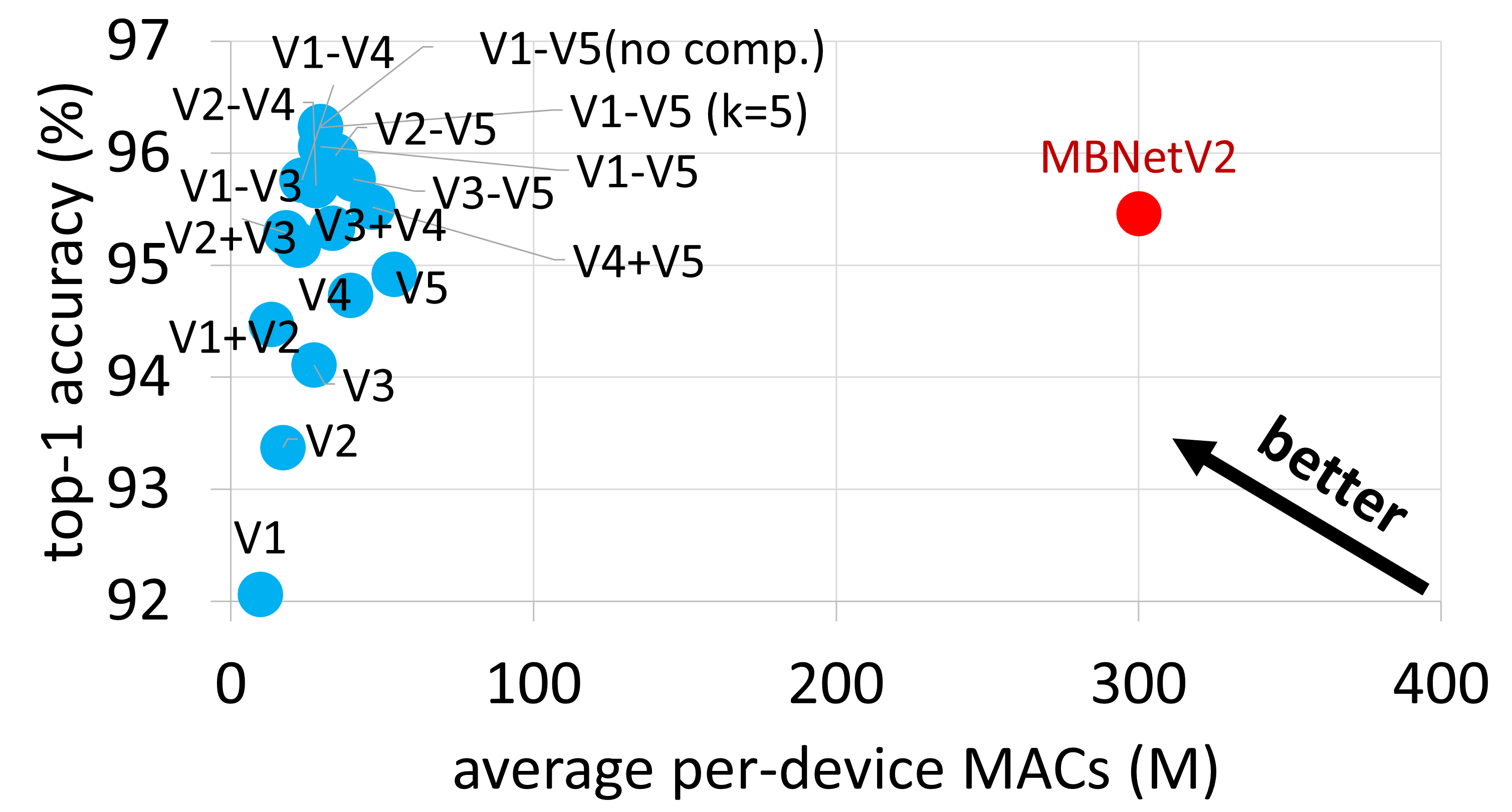
(a) CIFAR-10

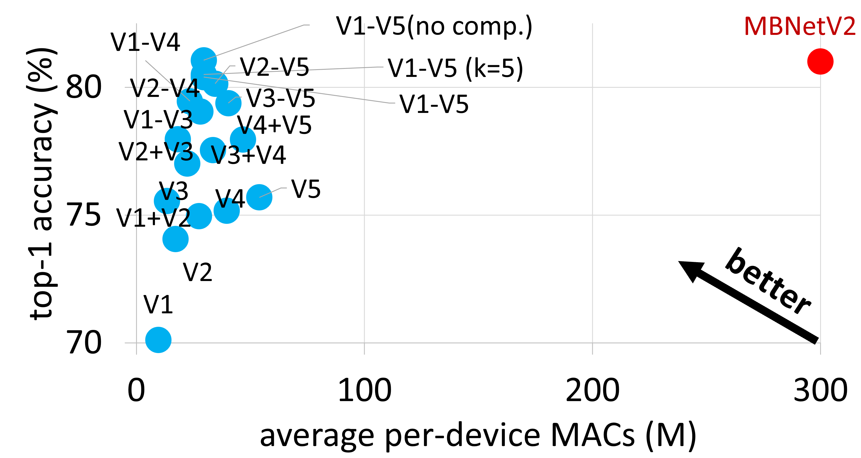
(b) CIFAR-100

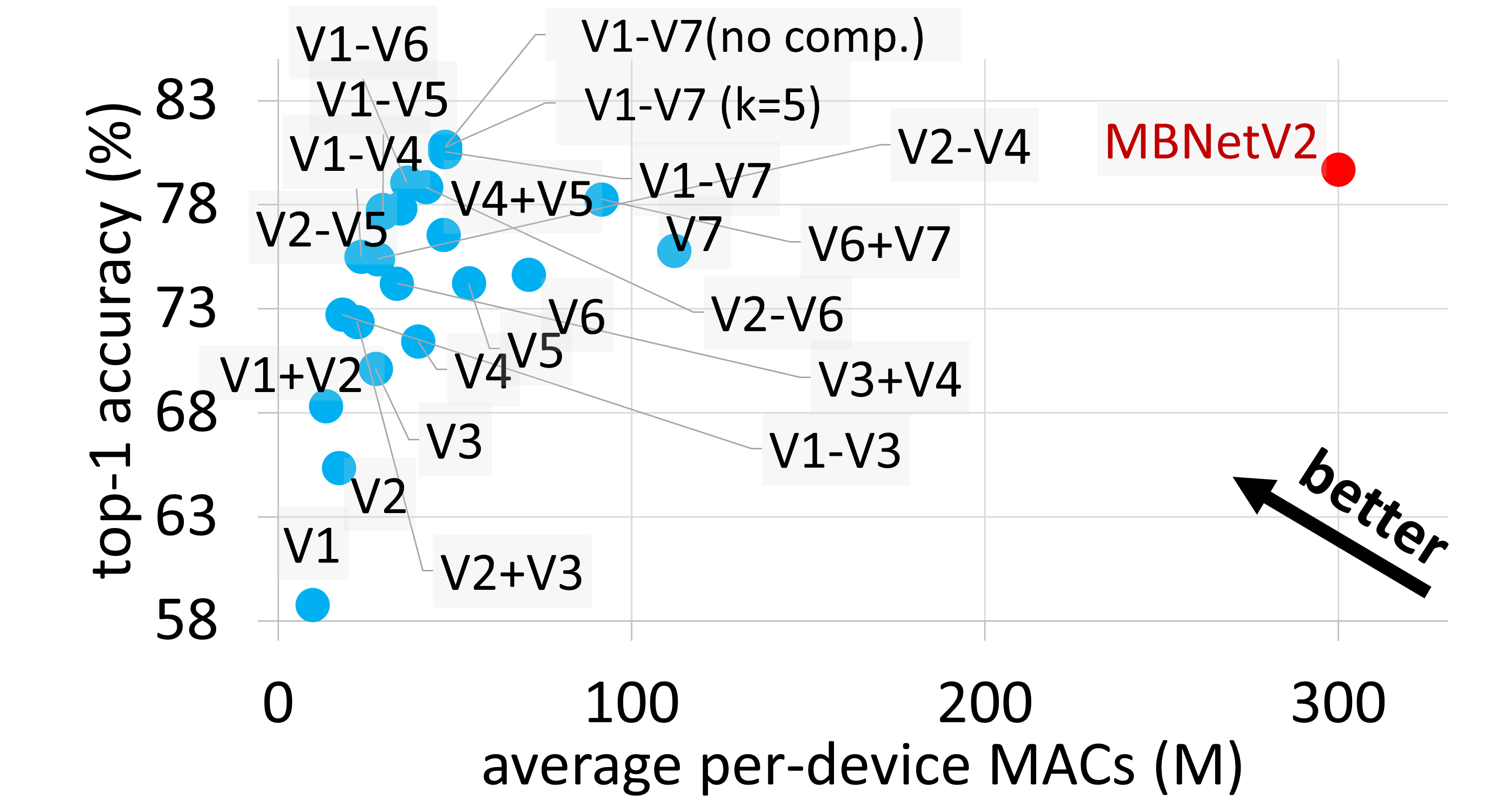
(c) Food-101

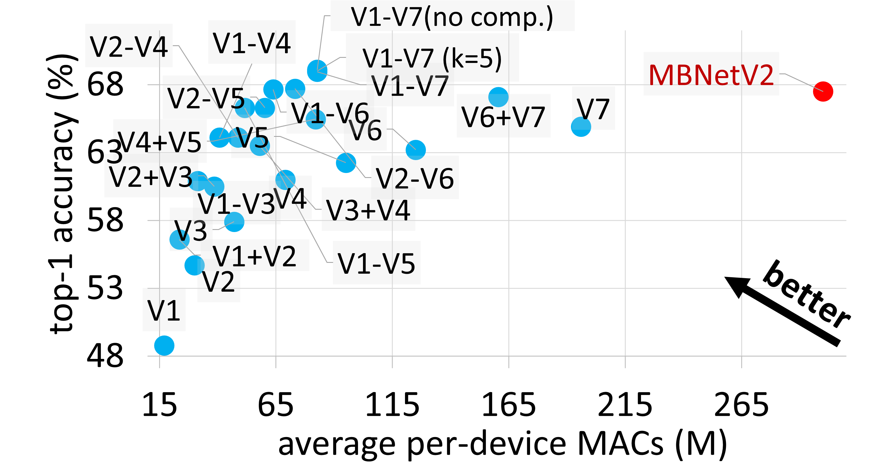
(d) ImageNet

Figure 6: Impact of each variant (and different combinations) on the final accuracy (Please zoom in).

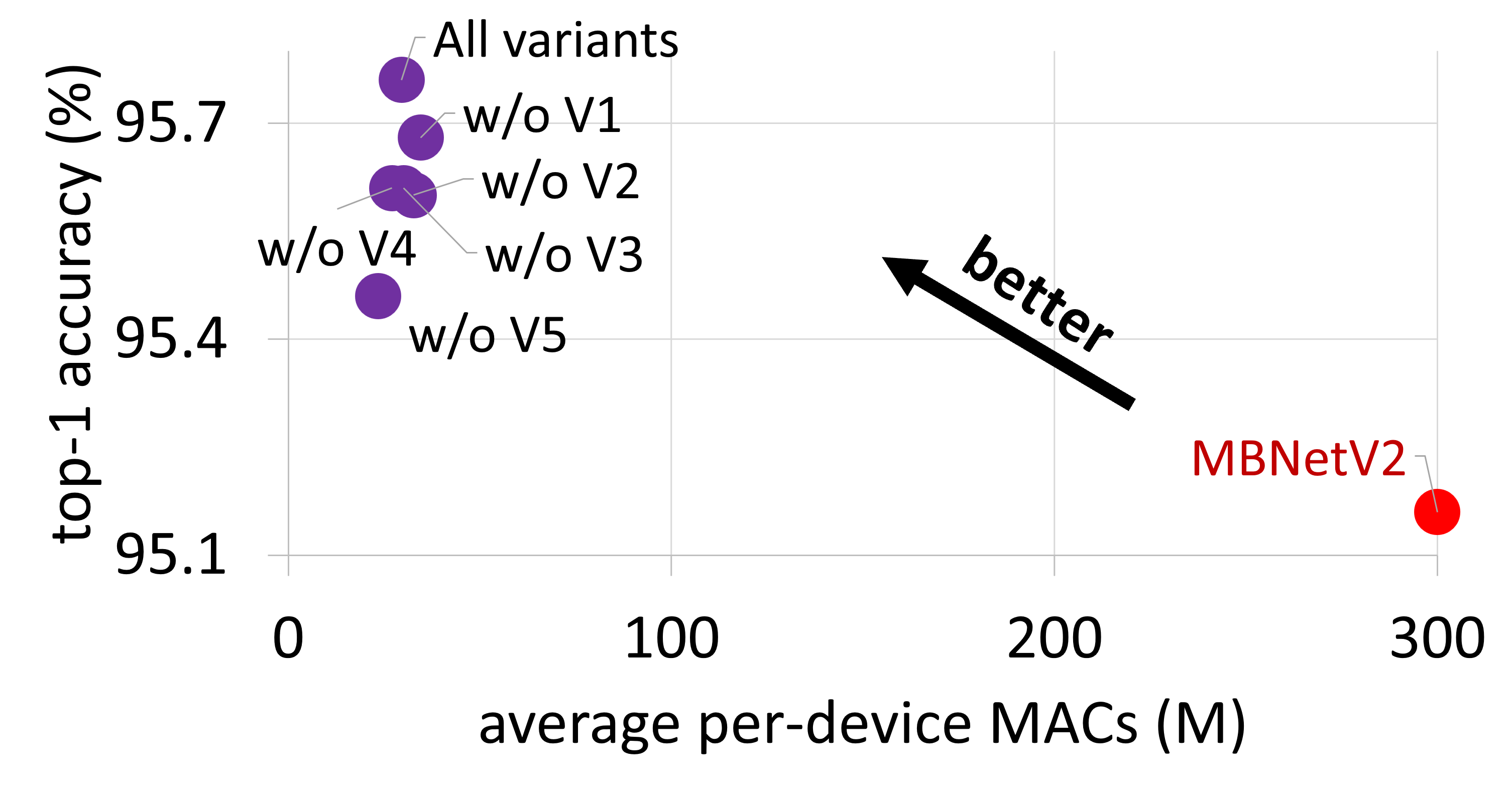
(a) CIFAR-10

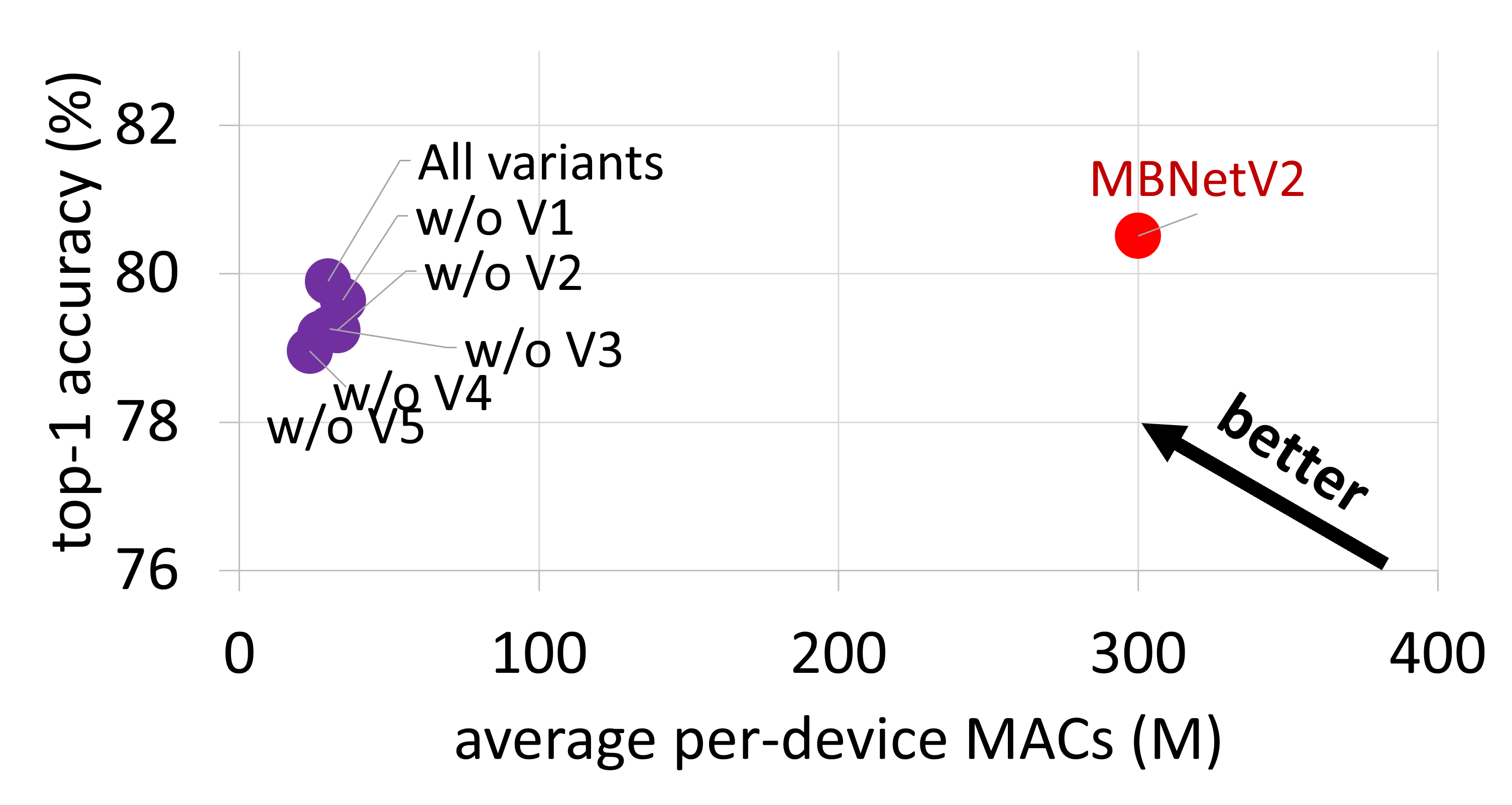
(b) CIFAR-100

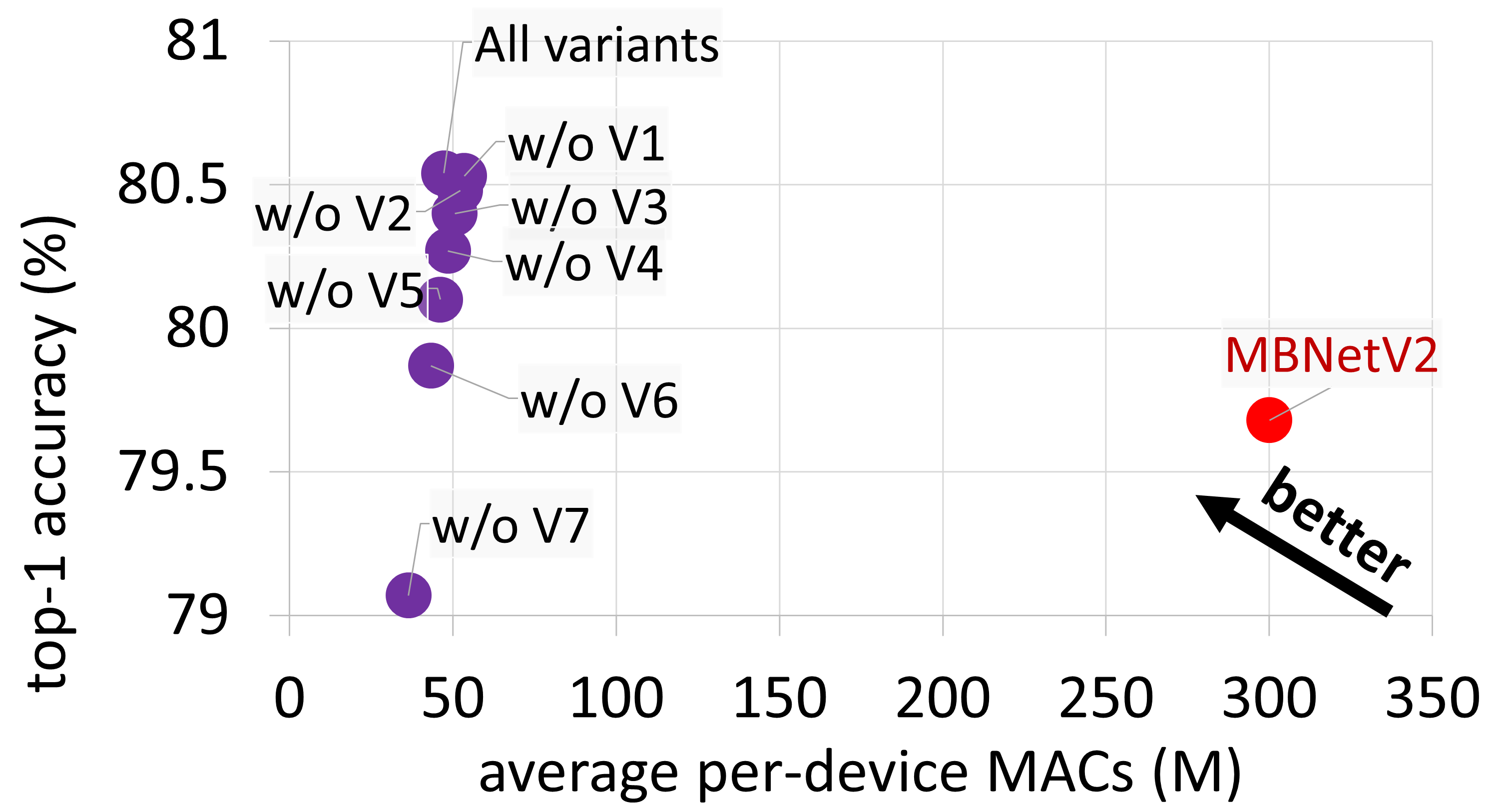
(c) Food-101

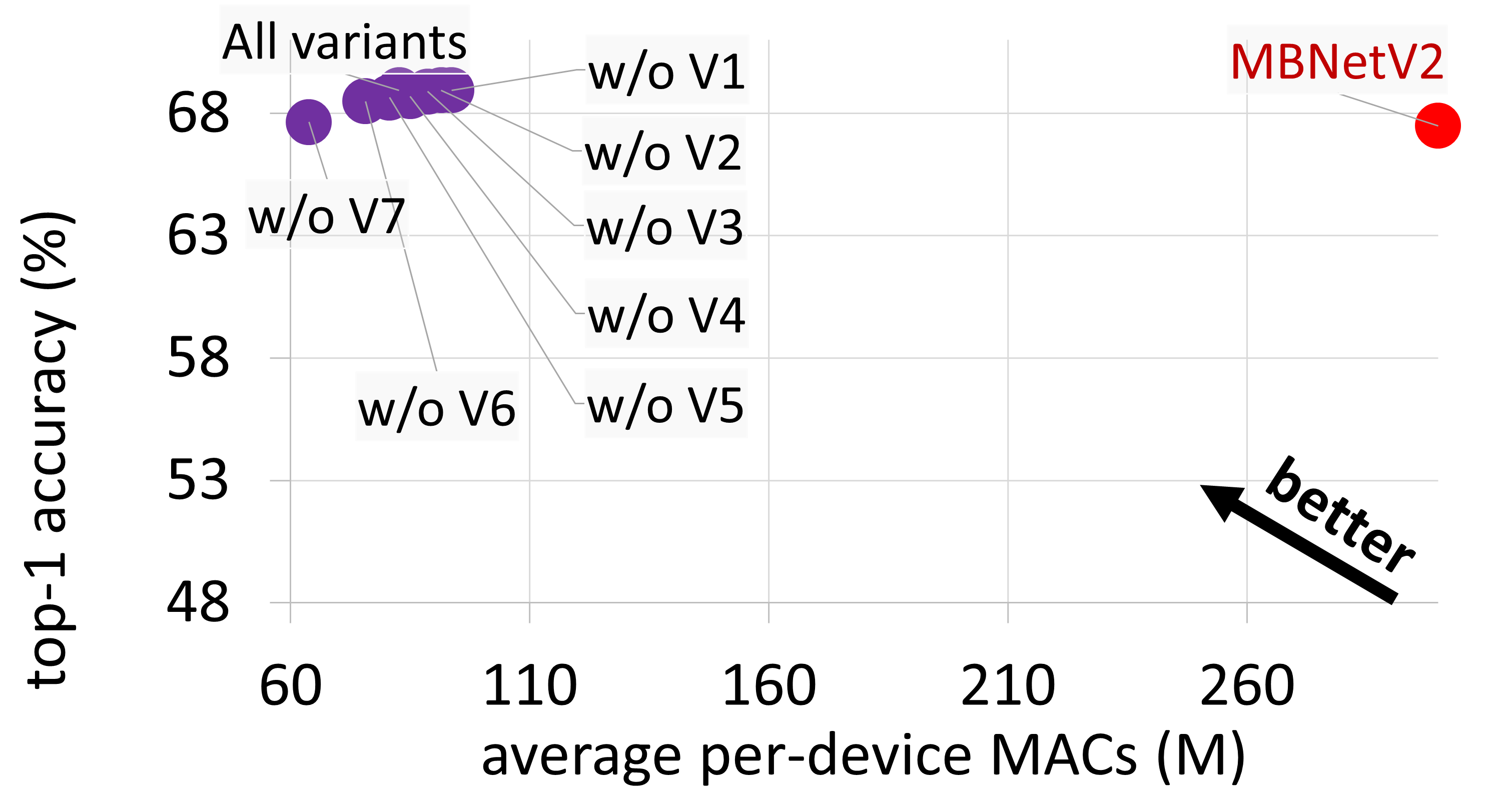
(d) ImageNet

Figure 7: How omitting a variant affects the final accuracy. (Please zoom in)

IV-G Availability in Presence of Failure

One serious drawback of utilizing idle nodes is preemption in presence of higher priority jobs (e.g., their main tasks). Missing real-time deadlines due to unexpected communication or computation issues are other reasons that indicate the demand for a fault-tolerant parallelism approach. Nevertheless, MP and CP need to get the results of all contributing machines to provide the final outcome. By design, our architecture is fault-tolerant even if $n\mathchar 45\relax 1$ worker nodes are not able to return their predictions. Our aggregation module also supports this behavior. As shown in Fig. 7, we can still have results by contribution of a fraction of variants being executed on different machines. As the number of faulty nodes increases (i.e., fewer contributing variants), the final accuracy decreases. The achievable accuracy depends on the variants remained for the aggregation. In the worst case, all nodes fail except the one that executes $V_{1}$ as it has the lowest accuracy among all, which is still better than MP/CP that fail to provide any predicton. Our VP can be viewed as providing a graceful degradation in presence of increasing levels of faults/preemptions in the environment.

IV-H Other Metrics: Inference Time, MACs, Model Size

We report the performance of our variants on the other common metrics. We convert each variant designed for and trained on Food-101 to TFLite [22], and execute them for $100$ iterations. The results are illustrated in Table VII. Since each variant has different characteristics, the slowest one determines the eventual response time. Therefore, depending on the available combination of nodes, one can get $2.5\mathchar 45\relax 13.2\times$ speedup compared to the baseline. Considering a smart home scenario with a star topology and the round-trip time ${RTT=2ms}$, the estimated speedup would be $2.4\mathchar 45\relax 10.7\times$

IV-I Variant Parallelism vs. Class Parallelism

We concisely compare our method with the current state-of-the-art deep learning parallelism algorithm, sensAI [6] which is a CP technique.

Fault-Tolerance: After sending requests to workers, the master node waits for a time window to receive as many responses as possible. Thus, in the event of preemtion due to processing high priority tasks or an issue in a worker or the network, the master node treats them as a fault. We demonstrated that in case of failure on even $n\mathchar 45\relax 1$ worker nodes, we can still get a response. In CP, however, since each model predicts different class(es), all contributing machines have to successfully process and send their results to the master. One can improve it by executing replications on additional machines, but it increases both complexity and cost. Another idea is to apply overlapping class-aware pruning [13]. In this type of replication, in presence of failure in one machine, the results can be aggregated from other machines with accuracy drop. Both ideas increase computation and communication costs.

Response Time, MACs, Model Size, Training Time: As depicted in Table VII, by leveraging class parallelism, sensAI can reach up to ${\sim}2\times$ speedup using $10$ parallel machines. We showed that variant parallelism gets ${\sim}2.5\mathchar 45\relax 3.2\times$ speedup compared with the baseline while requiring roughly half of in-parallel compute nodes compared to sensAI. Further note that, we trained our variants for $135$ epochs which is $32.5\%$ less than class parallelism, yet we achieve comparable or higher accuracy. However, since our infrastructures and scheduling policies are different, direct comparison might be unfair.

TABLE VII: Comparison of our variants with the baseline and sensAI.

Model	Time (ms)	Speedup	#MACs Gain	#Params Gain
MBNet2	$226\pm 0.5$	$1{\times}$	$1{\times}$	$1{\times}$
$V_{6}$	$91\pm 0.4$	$2.5\times$	$4.3\times$	$5.8\times$
$V_{5}$	$71\pm 0.2$	$3.2\times$	$5.6\times$	$6.1\times$
$V_{4}$	$53\pm 0.2$	$4.2\times$	$7.6\times$	$6.3\times$
$V_{3}$	$38\pm 0.2$	$5.9\times$	$10.9\times$	$6.7\times$
$V_{2}$	$26.5\pm 0.1$	$8.6\times$	$17.5\times$	$6.9\times$
$V_{1}$	$17\pm 0.05$	$13.2\times$	$31\times$	$7.1\times$
Aggregate	$0.05\pm 0$	-	-	-
sensAI	-	$2\times$	$3.5\times$	$5\times$

Output Size: In the tasks with few classes (e.g. CIFAR-10, SVHN, and MNIST) almost the same number of values must be transmitted. However, for the datasets with ${C>=100}$ (e.g. CIFAR-100 and Food-101), we transmit ten bytes per variant which depending on the number of clusters in CP, it can be up to $2\times$ ($20\times$ on ImageNet) less than sensAI.

Flexibility: Since each variant is being executed independently, it gives us more flexibility than CP to achieve different goals. We can generate additional variants based on more than one basic architecture, or design a highly customized variant for contributing machines. We can have several variants with different characteristics to be deployed on heterogeneous compute machines. VP can also be combined with other distribution schemes including CP.

V Conclusion & Future Directions

In this paper, we presented Variant Parallelism, a more flexible and fault-tolerant distribution scheme based on ensemble learning. Our evaluation on six different object recognition datasets demonstrates that our method can improve performance in number of parameters, MACs, and response time compared to the baseline and the current state-of-the-art. We note potential direction to be considered in future works. We intend to extend it to more complicated tasks such as object detection and semantic segmentation. We expect more performance gain is achievable when tasks become more complicated. Both VP and CP are based on the well-known ensemble learning techniques. Therefore, they can have similar weaknesses and strengths. For example, in VP combining variants with identical characteristics, may not help achieving significant accuracy boost unless we retrain each of them with different random seeds [23]. Contributing machines in CP and VP observe the same data. In some scenarios, e.g., a smart city with long latency or bandwidth bottlenecks, transmitting input data can impact the end-to-end latency. Combining split computing paradigm [24, 25] with CP or VP can help mitigate the problem. On that end, a hierarchy of resources with different computation and communication characteristics (e.g., end-edge-cloud) is another direction which has recently gained attention and has its own challenges [26, 27, 28]. For generating variants we apply untargeted structured pruning. Investigating targeted pruning methods (e.g., [29]) to further improve retraining and inference times, therefore, can be considered as part of the future work to this paper.

References

- [1] Z. Liu, H. Mao, C.-Y. Wu, C. Feichtenhofer, T. Darrell, and S. Xie, “A ConvNet for the 2020s,” in IEEE/CVF CVPR, 2022, pp. 11 976–11 986.
- [2] R. Bhardwaj, Z. Xia, G. Ananthanarayanan, J. Jiang, N. Karianakis, Y. Shu, K. Hsieh, V. Bahl, and I. Stoica, “Ekya: Continuous Learning of Video Analytics Models on Edge Compute Servers,” in USENIX NSDI, 2022.
- [3] M. Khani, G. Ananthanarayanan, K. Hsieh, J. Jiang, R. Netravali, Y. Shu, M. Alizadeh, and V. Bahl, “RECL: Responsive Resource-Efficient Continuous Learning for Video Analytics,” in USENIX NSDI, 2023.
- [4] M. Sandler, A. Howard, M. Zhu, A. Zhmoginov, and L.-C. Chen, “MobileNetV2: Inverted Residuals and Linear Bottlenecks,” in IEEE CVPR, 2018, pp. 4510–4520.
- [5] M. Tan and Q. Le, “EfficientNetV2: Smaller Models and Faster Training,” in ICML. PMLR, 2021, pp. 10 096–10 106.
- [6] G. Wang, Z. Liu, B. Hsieh, S. Zhuang, J. Gonzalez, T. Darrell, and I. Stoica, “sensAI: ConvNets Decomposition via Class Parallelism for Fast Inference on Live Data,” in MLSys, A. Smola, A. Dimakis, and I. Stoica, Eds., vol. 3, 2021, pp. 664–679.
- [7] J. Emmons, S. Fouladi, G. Ananthanarayanan, S. Venkataraman, S. Savarese, and K. Winstein, “Cracking open the DNN black-box: Video Analytics with DNNs across the Camera-Cloud Boundary,” in HotEdgeVideo, 2019, pp. 27–32.
- [8] X. Tan and I. Hakala, “StateOS: A Memory-Efficient Hybrid Operating System for IoT Devices,” IEEE Internet of Things Journal, 2023.
- [9] L. Zeng, X. Chen, Z. Zhou, L. Yang, and J. Zhang, “CoEdge: Cooperative DNN Inference with Adaptive Workload Partitioning over Heterogeneous Edge Devices,” IEEE/ACM Transactions on Networking, vol. 29, no. 2, pp. 595–608, 2020.
- [10] P. Yu and M. Chowdhury, “Fine-Grained GPU Sharing Primitives for Deep Learning Applications,” in MLSys, 2020.
- [11] J. Du, M. Shen, and Y. Du, “A Distributed In-Situ CNN Inference System for IoT Applications,” in IEEE ICCD, 2020, pp. 279–287.
- [12] H. Zhou, M. Li, N. Wang, G. Min, and J. Wu, “Accelerating Deep Learning Inference via Model Parallelism and Partial Computation Offloading,” IEEE Transactions on Parallel and Distributed Systems, vol. 34, no. 2, pp. 475–488, 2022.
- [13] Y. Yang, J. Chung, G. Wang, V. Gupta, A. Karnati, K. Jiang, I. Stoica, J. Gonzalez, and K. Ramchandran, “Robust Class Parallelism-Error Resilient Parallel Inference with Low Communication Cost,” in IEEE ASILOMAR, 2020, pp. 1064–1065.
- [14] A. G. Howard, M. Zhu, B. Chen, D. Kalenichenko, W. Wang, T. Weyand, M. Andreetto, and H. Adam, “MobileNets: Efficient Convolutional Neural Networks for Mobile Vision Applications,” arXiv:1704.04861, 2017.
- [15] J. Deng, W. Dong, R. Socher, L.-J. Li, K. Li, and L. Fei-Fei, “ImageNet: a Large-Scale Hierarchical Image Database,” in IEEE CVPR, 2009, pp. 248–255.
- [16] A. Krizhevsky and G. Hinton, “Learning Multiple Layers of Features from Tiny Images,” 2009.
- [17] H. Xiao, K. Rasul, and R. Vollgraf, “Fashion-MNIST: a Novel Image Dataset for Benchmarking Machine Learning Algorithms,” arXiv:1708.07747, 2017.
- [18] Y. LeCun, C. Cortes, and C. J. Burges, “The MNIST Database of Handwritten Digits,” ATT Labs. Available: yann.lecun.com/exdb/mnist, vol. 2, 2010.
- [19] Y. Netzer, T. Wang, A. Coates, A. Bissacco, B. Wu, and A. Y. Ng, “Reading Digits in Natural Images with Unsupervised Feature Learning,” 2011.
- [20] L. Bossard, M. Guillaumin, and L. Van Gool, “Food-101 - Mining Discriminative Components with Random Forests,” in ECCV. Springer, 2014, pp. 446–461.
- [21] “TFLite Model Benchmark Tool with C++ Binary,” 2022. [Online]. Available: github.com/tensorflow/tensorflow/tree/master/tensorflow/lite/tools/benchmark
- [22] “TensorFlow Lite,” 2022. [Online]. Available: tensorflow.org/lite
- [23] Z. Allen-Zhu and Y. Li, “Towards Understanding Ensemble, Knowledge Distillation and Self-Distillation in Deep Learning,” arXiv:2012.09816, 2020.
- [24] Y. Kang, J. Hauswald, C. Gao, A. Rovinski, T. Mudge, J. Mars, and L. Tang, “Neurosurgeon: Collaborative Intelligence Between the Cloud and Mobile Edge,” ACM SIGARCH Computer Architecture News, vol. 45, no. 1, pp. 615–629, 2017.
- [25] M. Sbai, M. R. U. Saputra, N. Trigoni, and A. Markham, “Cut, Distil and Encode (CDE): Split Cloud-Edge Deep Inference,” in IEEE SECON, 2021, pp. 1–9.
- [26] N. Asadi and M. Goudarzi, “An Ensemble Mobile-Cloud Computing Method for Affordable and Accurate Glucometer Readout,” arXiv:2301.01758, 2023.
- [27] H. Zhou, Z. Zhang, D. Li, and Z. Su, “Joint Optimization of Computing Offloading and Service Caching in Edge Computing-Based Smart Grid,” IEEE Transactions on Cloud Computing, 2022.
- [28] H. Zhou, T. Wu, X. Chen, S. He, D. Guo, and J. Wu, “Reverse Auction-Based Computation Offloading and Resource Allocation in Mobile Cloud-Edge Computing,” IEEE Transactions on Mobile Computing, 2022.
- [29] K. Zhao, A. Jain, and M. Zhao, “Automatic Attention Pruning: Improving and Automating Model Pruning using Attentions,” in AISTATS, 2023, pp. 10 470–10 486.