A Policy-Guided Imitation Approach for
Offline Reinforcement Learning
Abstract
Offline reinforcement learning (RL) methods can generally be categorized into two types: RL-based and imitation-based. RL-based methods could in principle enjoy out-of-distribution generalization but suffer from erroneous off-policy evaluation. Imitation-based methods avoid off-policy evaluation but are too conservative to surpass the dataset. In this study, we propose an alternative approach, inheriting the training stability of imitation-style methods while still allowing logical out-of-distribution generalization. We decompose the conventional reward-maximizing policy in offline RL into a guide-policy and an execute-policy. During training, the guide-policy and execute-policy are learned using only data from the dataset, in a supervised and decoupled manner. During evaluation, the guide-policy guides the execute-policy by telling where it should go so that the reward can be maximized. By doing so, our algorithm allows state-compositionality from the dataset, rather than action-compositionality conducted in prior imitation-style methods. We dumb this new approach Policy-guided Offline RL (POR). POR demonstrates the state-of-the-art performance on D4RL, a standard benchmark for offline RL. We also highlight the benefits of POR in terms of improving with supplementary suboptimal data and easily adapting to new tasks by only changing the guide-policy. Code is available at https://github.com/ryanxhr/POR.
1 Introduction
Offline RL, also known as batch RL, allows learning policies from previously collected data, without online interactions [30; 32]. It is a promising area for bringing RL into real-world domains, such as robotics [22], healthcare [48] and industrial control [63]. In such scenarios, arbitrary exploration with untrained policies is costly or dangerous, but sufficient prior data is available. While most off-policy RL algorithms are applicable in the offline setting by filling the replay buffer with offline data, improving the policy beyond the level of the behavior policy often entails querying the value function (i.e., Q function) about values of actions that were not seen in the dataset. Those out-of-distribution actions can be deemed as adversarial examples of the Q function [29], which cause extrapolation error of the Q-function. The error will be accumulated by the deadly triad issue [50], propagate across the state-action space through the iterative dynamic programming procedure [5], and can not be eliminated without requiring a growing batch of online samples [32].
To alleviate this issue, prior model-free offline RL methods typically add a behavior regularization term to the policy improvement step, to limit how far it deviates from the behavior policy. This can be achieved explicitly by calculating some divergence metrics [27; 54; 39; 14], or implicitly by regularizing the learned value functions to assign low values to out-of-distribution actions [29; 25; 1; 3]. Nevertheless, this imposes a trade-off between accurate value estimation (more behavior regularization) and maximum policy improvement (less behavior regularization). To avoid this problem, recently a branch of methods bypass querying the values of unseen actions by performing some kind of imitation learning on the dataset***The core difference between RL-based and imitation-based methods is that RL-based methods learn a value function of policy while imitation-based methods don’t.. This can be achieved by filtering trajectories based on their return [41; 8], or reweighting transitions based on how advantageous they could be under the behavior policy [5; 26], or just be conditioned on some variables without any dataset reweighting [7; 10]. Although imitation-style methods enjoy a stable training process and are able to effectively perform multi-step dynamic programming by assigning the proper reweighting weight or conditioned variable [26; 10], they only allow action-compositionality from the dataset, lose the ability to surpass the dataset by out-of-distribution generalization, which only appears in RL-based methods.
In this work, we propose an alternative approach. We aim at inheriting the training stability of imitation-style methods while still allowing logical out-of-distribution generalization. To do so, we propose Policy-guided Offline RL (POR), an algorithm that employs two policies to solve tasks: a guide-policy and an execute-policy. The job of the guide-policy is to learn the optimal next state given the current state, and the job of the execute-policy is to learn how different actions can produce different next states, given the current state. By this manner, we decompose the original task of RL (i.e., reward-maximizing) into two distinct yet complementary tasks, and this decomposition makes each task much easier to be solved. During evaluation, the guide-policy serves as a guide for the execute-policy by telling it where to go so that the reward can be maximized. By doing so, our algorithm allows state-compositionality from the dataset, rather than action-compositionality conducted in prior work, which owns logical out-of-distribution generalization.
Our method is easy to implement by only adding the learning of a guide-policy, the training stage of the guide-policy and execute-policy are decoupled, using in-sample learning from the dataset. We test POR in widely-used D4RL offline RL benchmarks and demonstrates the state-of-the-art performance, especially on low-quality datasets that require out-of-distribution generalization to achieve a high score. We also show that by decoupling the learning of guide-policy and execute-policy, we can enhance the guide-policy with supplementary suboptimal data, or re-learn the guide-policy to adapt to new tasks with different reward functions, without changing the execute-policy.
2 Related Work
RL-based offline approach A large portion of offline RL methods is RL-based. RL-based methods typically augment existing off-policy methods (e.g., Q-learning or actor-critic) with a behavior regularization term. The primary ingredient of this class of methods is to propose various policy regularizers to ensure that the learned policy does not stray too far from the behavior policy. These regularizers can appear explicitly as divergence penalties [54; 27; 14], implicitly through weighted behavior cloning [52; 41; 39], or more directly through careful parameterization of the policy [15; 66]. Another way to apply behavior regularizers is via modification of the critic learning objective to incorporate some form of regularization to encourage staying near the behavioral distribution and being pessimistic about unknown state-action pairs [38; 29; 25; 59]. There are also several works incorporating behavior regularization through the use of uncertainty. The uncertainty quantification can be done via Monte Carlo dropout [55] or explicit ensemble models [3; 62; 23; 64]. Note that the behavior regularization weight is crucial in RL-based methods. With a small weight, RL-based methods could in principle enjoy out-of-distribution generalization since they perform true dynamic programming. However, a small weight will make erroneous off-policy evaluation due to distribution shift and the policy is extremely vulnerable to the value function misestimation.
Imitation-based offline approach Another line of methods, on the contrary, performs some kind of imitation learning on the dataset, without the need to do off-policy evaluation. When the dataset is good enough or contains high-performing trajectories, we can simply clone the actions observed in the dataset [43], or perform some kind of filtering or conditioning to extract useful transitions. For instance, recent work filters trajectories based on their return [8; 41], or directly filters individual transitions based on how advantageous these could be under the behavior policy and then clones them [5; 26; 6; 17; 57]. Conditioned BC methods are based on the idea that every transition or trajectory is optimal when conditioned on the right variable [16; 10]. In this way, after conditioning, the data becomes optimal given the value of the conditioned variable. The conditioned variable could be the cumulative return [7; 20; 28], or the goal information if provided [35; 16; 10; 60]. A recent study [10] shows that goal-conditioning can be super useful in D4RL AntMaze datasets. However, this introduces the assumption that we have some prior information about the structure of the task, which is beyond the standard offline RL setup.
Our method can be viewed as a combination of RL-based and imitation-based methods. We adopt an imitation-style manner to train the goal-policy and execute-policy. During evaluation, however, following the guide-policy, the execute-policy could produce out-of-distribution actions by leveraging the generalization capacity of the function approximator.
3 Preliminaries
Offline RL We consider the standard fully observed Markov Decision Process (MDP) setting [47]. An MDP can be represented as where is the state space, is the action space, is the transition probability distribution function, is the reward function, is the initial state distribution and is the discount factor, we assume in this work. The goal of RL is to find a policy that maximizes the expected cumulative discounted reward (or called return) along a trajectory as
| (1) |
In this work, we focus on the offline setting. The goal is to learn a policy from a fixed dataset consisting of trajectories that are collected by different policies, where is the time horizon. The dataset can be heterogenous and suboptimal, we denote the underlying behavior policy of as , which represents the conditional distribution observed in the dataset.
RL via Supervised Learning Conventional RL methods generally either compute the derivative of (1) with respect to the policy directly via policy gradient methods [44; 21], or estimate a value function or Q-function by means of TD learning [53], or both [45; 18]. In the RL via Supervised Learning framework, we avoid the complex and potentially high-variance policy gradient estimators, as well as the complexity of temporal difference learning. Instead, we perform conditioned behavior cloning on some extra information, such as goal state, cumulative return, or language description [35; 16]. When applying the framework to the offline RL setting, we can take the offline dataset as input and find the outcome-conditioned policy that optimizes
| (2) |
where is an outcome conditioned on the remaining trajectory, i.e., , and we use to denote a fragment of the trajectory.
4 Policy-guided Offline Reinforcement Learning
We now continue to describe our proposed approach, POR. To have a clear understanding of the out-of-distribution generalization of POR, we begin with a motivating example which demonstrates that by allowing state-compositionality on the dataset, the agent is able to generalize to a much better policy than doing action-compositionality. Then we describe how we accomplish this idea in the more general case and introduce the algorithm details of POR. Finally, we give a theoretical analysis of POR, we are interested to see how close the policy induced by POR and the optimal policy could be.
4.1 A Motivating Example
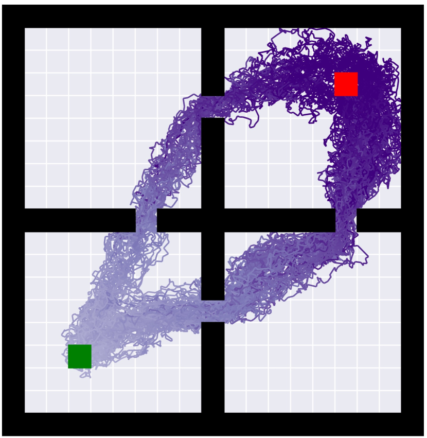
We first use a simple, didactic toy example to illustrate the importance of state-stitching for offline RL. Let’s consider the navigation task shown in Figure 1, where the goal is to find the shortest path from the starting location (bottom-left corner) to the goal location (top-right corner) in the grid world. The state and action space in this task are discrete, the state consists of the coordinate and the agent could choose to move to any of its nearby 8 grids (i.e., the action space is 8). The agent receives a reward of for entering the goal state and for all other transitions. The offline dataset (green-arrowed lines) consists of two suboptimal trajectories from the start location to the goal location, plus transitions of taking random actions at random states.
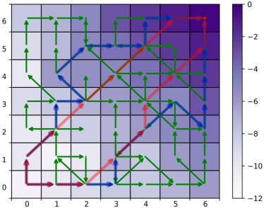
We use the grid color (more saturated to purple means higher value) to show the value function computed from the offline dataset. We compare two methods that use the value function differently. At a state , the first method chooses the action in the dataset that leads to with the highest ; the second method chooses the action that leads to in the dataset with the highest , note that is not necessarily to be within the dataset. The first method is doing action "stitching" in the dataset while the second method is doing state "stitching". Although both methods are able to "stitch" suboptimal trajectories together from the dataset and successfully travel from the start location to the goal location, the action-stitching method takes more steps (11 steps) compared with the state-stitching method (7 or 8 steps), as shown in Figure 1.
The action-stitching method introduced above is actually an abstract methodology of imitation-based methods, which imitate the transitons in the dataset unequally with different weight choices. However, these methods are too conservative to find the optimal trajectory, especially when there does not exist one in the offline dataset. To generate better-than-dataset trajectories (e.g., red-arrowed lines), the agent needs to take logical out-of-distribution actions.
Note that in the toy example, we give the agent the freedom to choose any action that leads to the highest-value state in the dataset. This allows the most out-of-distribution generalization and is realizable in some simple tasks (e.g., discrete state and action space) with high action coverage, for instance, in the toy example, given historical results at , the agent can successfully recognize that taking upper-right will arrive at . However, in the more general case, especially the continuous state and action space setting, this may make the agent do erroneously-generalized actions as the same state can hardly be observed twice. To perform logical out-of-distribution generalization, we need a Prophet, i.e., the guide-policy, to help the agent by telling it which state it should (high reward) and can (logical generalization) go to. It turns out that the involvement of the guide-policy also brings some theoretical meaning, we will discuss that in Section 4.4.
4.2 Learning the Guide-Policy
Recall that the goal of the guide-policy is to guide the execute-policy about which state it should go to. To accomplish that, we train a state value function . The training of uses only samples in the offline dataset, it doesn’t suffer from overestimation because there’re no out-of-distribution actions involved. To approximate the optimal value function in the dataset, we adopt tricks from recent work [26; 36] by giving the loss with a different weight using expectile regression, yielding the following asymmetric loss
| (3) |
It can be seen that when , this operator is reduced to Bellman expectation operator, while when , this operator approaches Bellman optimality operator. Note that our learning objective bears similarity with IQL [26], however, here we aim to learn a state value function while IQL aims to learn a state-action value function so as to extract the policy. To do this, IQL needs to learn both and ( is used to isolate the effect of state and approximate the expectile of only with respect to the action distribution), the training of and are coupled and may affect each other.
Inspired by recent work [56] that enables in-sample learning via implicit value regularization, we additionally propose a sparse value learning objective for , which is a more principled way to approximate the optimal in the dataset while preventing from distributional shift, by
| (4) |
We denote this version of POR as POR-sparse. In POR-sparse, controls the trade-off between approximating the optimal and reducing the approximation error, a smaller drives towards a better whereas introducing larger approximation error, and vice versa.
Simply maximizing the guide-policy with respect to will result in a state where the execute-policy may make erroneous generalization. To alleviate this issue, we add a behavior constraint term to the learning objective of the guide-policy. Denote the guide-policy as , the learning objective is given by
| (5) |
where is an estimated behavior guide-policy from the dataset. The weight serves as the trade-off between guiding to space with high-reward and space that the execute-policy ought to have a correct generalization. We also give an alternative learning objective that implicitly involves the behavior constraint by using the residual () as the behavior cloning weight [42; 41], which bypasses the need to estimate by
| (6) |
4.3 Learning the Execute-Policy: Training and Evaluation
After learning the guide-policy, now we turn to the execute-policy. Since the job of the execute-policy is to have a strong generalization ability, we adopt the RL via Supervised Learning framework by conditioning the execute-policy on that encountered in the dataset. To be more specific, denote the execute-policy as . During training, performs supervised learning by maximizing the likelihood of the actions given the states and next states, yielding the following objective
| (7) |
in some scenarios with low data quality, one can also add the exponential residual weight in objective (6) to (7) to mitigate the effect of those bad actions.
During evaluation, given a state , the final action is determined by both the guide-policy and the execute-policy, by
| (8) |
Note that our learning objective (7) differs from previous RL via Supervised Learning methods in that we only use the next state as the conditioned variable, there’s no need to estimate the cumulative return [7], which may be highly suboptimal in certain cases [11; 4]. Our method also works in settings where we don’t know the goal information [10]. Also, during evaluation, previous methods show that the choice of conditioned variable is crucial important as little changes will cause significant performance difference [7]. In our method, owing to the existence of the guide-policy, the optimal conditioned variable can be automatically generated.
Our final algorithm, POR, consists of three supervised stages: learning , learning , and learning . We summarize the training and evaluation procedure of POR in Algorithm 1. Note that the training of and are fully decoupled, this brings POR some nice properties to improve with supplementary data or transfer to new tasks, we will further investigate it in the experiments.
4.4 Analysis
In this section, we give a theoretical analysis of POR. Concretely, we aim to 1) give the lower bound of the performance difference between POR and the optimal policy , and 2) analyze how the guide-policy will influence this bound.
We begin by introducing the notation and assumptions used in our analysis. We denote as the inverse transition operator. We denote and as the ground truth of and , respectively. We also denote as the upper bound of the approximation error in the dataset during training. We then introduce the following two assumptions.
Assumption 1.
(Non-lazy MDP) The inverse transition operator is -Lipschitz continuous, i.e., .
Assumption 2.
(Lipschitz continuous function approximators) The execute-policy we trained is -Lipschitz continuous, i.e., .
Assumption 1 holds when actions do have effects on state transitions (i.e. if , then ). We refer the MDP that satisfies Assumption 1 as non-lazy MDP and others as lazy MDP. It should be mentioned that most real-world tasks belong to the non-lazy MDP case, it is meaningless to study under the lazy MDP case because in lazy MDP, action changes will have little effect on state transitions, making the policy learning in vain. Assumption 2 is a mild assumption that is frequently utilized in plenty of works [51; 37; 33].
Then in Theorem 1, we show that under these two assumptions, the gap between the optimal action and the action output by POR can be bounded.
Theorem 1.
(Single step gap to optimal action). The single-step gap between optimal action and the action induced by our method can be bounded as
| (9) |
Theorem 1 states that single step optimal gap is related to three parts: . is the generalization performance factor. It can be found that a small value of enables a small , which indicates the necessity to constrain the guide-policy to stay close to the dataset. denotes the suboptimality constant. Intuitively, a loosened constraint on the guide-policy may induce a small suboptimality constant but on the other hand, may suffer from the risk of a high value of . The guide-policy serves as a trade-off between and , we could balance the constraint strength and suboptimality by adjusting in Eq.(5) to obtain the lowest bound. is related to the approximation error on the training data, which can be reduced via improving the representation ability of function approximators but may suffer from a high due to the overfitting caused by over-parameterization. also depends on the Lipschitz constant and . Note that a smooth inverse transition operator will result in a small value of and (because is trained to approximate ), this means our method may achieve better performance under a smoother inverse transition.
5 Experiments
We present empirical evaluations of POR in this section. We first evaluate POR against other baseline algorithms on D4RL [13] benchmark datasets. We then explore deeper on the guide-policy about the benefits of the decoupled training process. We finally establish ablation studies on the execute-policy.
5.1 Comparative Experiments on D4RL Benchmark Datasets
| D4RL Dataset |
|
|
Best RL Baseline | ||||||
| 10%BC | One-step | IQL | DT | RvS | POR (ours) | ||||
| antmaze-u | 62.8 | 64.3 | 87.5 2.6 | 59.2 | 65.4 |
|
|||
| antmaze-u-d | 50.2 | 60.7 | 66.2 13.8 | 53.0 | 60.9 | 71.3 12.1 | |||
| antmaze-m-p | 5.4 | 0.3 | 71.2 7.3 | 0 | 58.1 | 84.6 5.6 | |||
|
9.8 | 0 | 70.0 10.9 | 0 | 67.3 | 79.2 3.1 | |||
| antmaze-l-p | 0 | 0 | 39.6 5.8 | 0 | 32.4 | 58.0 12.4 | |||
| antmaze-l-d | 0 | 0 | 47.5 9.5 | 0 | 36.9 | 73.4 8.5 | |||
| antmaze mean | 21.4 | 20.8 | 63.6 8.3 | 18.7 | 53.5 | 76.2 8.1 | 58.4 | ||
| halfcheetah-m |
|
48.4 0.1 | 47.4 0.2 | 42.6 0.1 | 41.6 | 48.8 0.5 | |||
| hopper-m | 56.9 | 59.6 2.5 | 66.2 5.7 | 67.6 1.0 | 60.2 | 78.6 7.2 | |||
| walker2d-m | 75.0 | 81.8 2.2 | 78.3 8.7 | 74.0 1.4 | 71.7 | 81.1 2.3 | |||
| halfcheetah-m-r | 40.6 | 38.1 1.3 | 44.2 1.2 | 36.6 0.8 | 38.0 | 43.5 0.9 | |||
| hopper-m-r | 75.9 | 97.5 0.7 | 94.7 8.6 | 82.7 7.0 | 73.5 | 98.9 2.1 | |||
| walker2d-m-r | 62.5 | 49.5 12.0 | 73.8 7.1 | 66.6 3.0 | 60.6 | 76.6 6.9 | |||
| halfcheetah-m-e | 92.9 | 93.4 1.6 | 86.7 5.3 | 86.8 1.3 | 92.2 | 94.7 2.2 | |||
| hopper-m-e | 110.9 | 103.3 1.9 | 91.5 14.3 | 107.6 1.8 |
|
90.0 12.1 | |||
|
109.0 | 113.0 0.4 | 109.6 1.0 | 108.1 0.2 | 106.0 | 109.1 0.7 | |||
| locomotion mean | 55.5 | 58.2 2.0 | 57.6 6.6 | 56 1.4 | 53.7 | 65.6 2.7 | 63.5 | ||
| Algorithm | antmaze-u | antmaze-u-d | antmaze-m-p | antmaze-m-d | antmaze-l-p | antmaze-l-d |
| POR | 90.6 10.7 | 71.3 12.2 | 84.6 5.6 | 79.2 3.1 | 58.0 12.4 | 73.4 8.5 |
| POR-Sparse | 95.0 3.4 | 86.3 6.1 | 82.4 5.5 | 71.0 2.4 | 48.8 4.1 | 53.4 3.6 |
We first evaluate our approach on D4RL MuJoCo and AntMaze datasets [13]. Notice that most of MuJoCo datasets (except random and medium datasets) consist of a large fraction of near-optimal trajectories, while AntMaze datasets contain few or no near-optimal trajectories. Hence those low-quality datasets can serve as a good testbed for quantifying the compositionality ability.
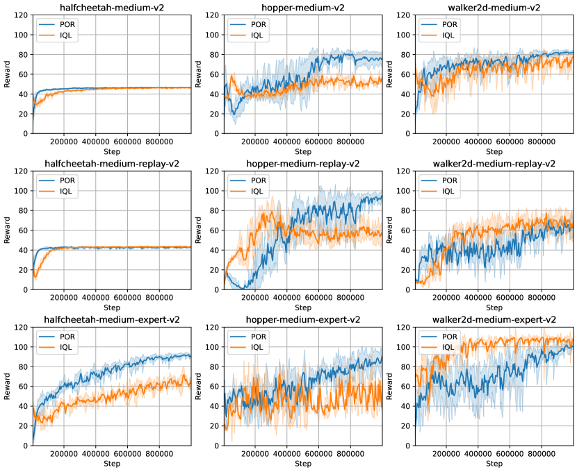
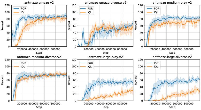
We compare POR with both RL-based and imitation-based baselines. For RL-based baselines, we select the best one from 5 state-of-the-art algorithms, including BCQ [15], BEAR [27], BRAC [54], CQL [29] and TD3+BC [14]. For imitation-based baselines, we further split them into Weighted BC methods and Conditioned BC methods. Weighted BC methods include 10%BC [7], One-step RL [5] and IQL [25]. 10%BC is a filtered version of BC that runs behavior cloning on only the top 10% high-return trajectories in the dataset. One-step RL and IQL can be viewed as using different weights to do behavior cloning (see Appendix A for discussion). Conditioned BC methods include DT [7] and RvS [10]. DT is built with Transformer and conditioned on the cumulative return. RvS well studied the effect of different conditional information on different tasks. The score of RvS is chosen by the higher score between RvS-R and Rvs-G, which use the reward-to-go and oracle goal information as the conditioned variable, respectively. Note that we also categorize our method POR into conditioned BC methods because the execute-policy is learned in a similar manner to other conditioned BC methods. Note that the results of Filter BC are from our own implementation, and the results of IQL on MuJoCo random tasks are re-runed using the author-provided implementation. Other results are taken directly from their corresponding papers. To enable fairness and consistency in the evaluation process, we train our algorithm for 1 million time steps and evaluate every 5000 time steps that consist of 10 episodes. Full experimental details are included in Appendix D.1, learning curves of POR against our implemented IQL (using the same codebase and network structures) and other ablation studies can be found in Appendix E and Appendix F, respectively.
The results are shown in Table 1, in MuJoCo locomotion tasks, POR performs competitively to the best performance of prior methods in high-quality datasets, while achieving much better performance than other methods in low-quality datasets (e.g., medium datasets). On the more challenging AntMaze tasks, POR outperforms all other baselines by a large margin. It even surpassed RvS that uses the oracle goal information to learn the policy. We conjecture that the success in all those datasets should be credited to the out-of-distribution generalization ability of POR. We also compare POR-sparse with POR, in some AntMaze tasks, the performance of POR-sparse even surpasses that of POR.
5.2 Validation Experiments on Out-of-Distribution Generalization
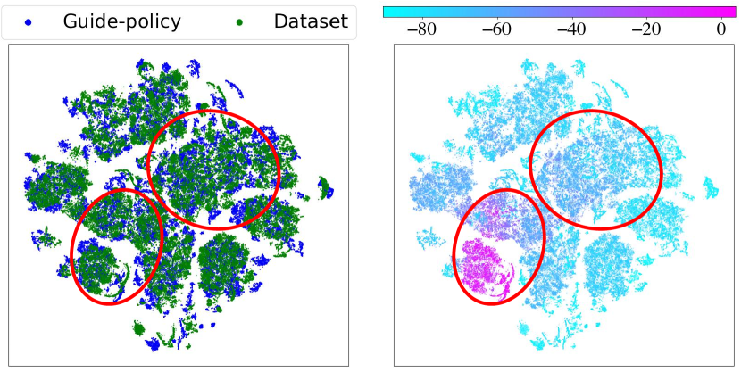
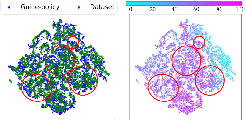
In this section, we try to validate our hypothesis about the out-of-distribution generalization of POR. We are especially interested to see how the guide-policy is learned in those high-dimensional tasks in D4RL. To do so, we compare the distribution of generated by the guide-policy with the distribution of from the offline dataset. We choose antmaze-large-diverse and hopper-medium-replay, two datasets for evaluation. For each dataset, we randomly collect transition tuples. To visualize the results clearly, we plot the distribution of and with t-Distributed Stochastic Neighbor Embedding (t-SNE) [19], we also visualize the true values of all states using the optimal value function .
The results are shown in Figure 2, it can be found that in both tasks, the distribution of bears some similarity to the distribution of . However, when looking at the non-overlapped area of and , we found that has a much higher value than , especially in the antmaze-large-diverse dataset. Those out-of-distribution and high-value areas are exactly where POR generalized to, note that the high-value benefit of the single-step generalization could also be accumulated and propagated through time steps, resulting in a much better policy.
5.3 Investigations on the Guide-Policy
In this section, we investigate what is the potential benefit of decoupling the training process of the guide-policy and execute-policy. We found that as the execute-policy is not task-specific and only cares about the effect of actions on different states, one can reuse its powerful generalization ability when encountered with additional suboptimal data or adapting to a new task. We only need to re-train the guide-policy as it is task-specific.
Improve guide-policy by additional suboptimal data We first study the setting where we already have a policy learned from a small yet high-quality dataset , and now we get a supplementary large dataset . may be sampled from one or multiple behavior policies, it provides higher data coverage but could be suboptimal. We are interested to see whether we can use to obtain a better policy. This setting is realistic as low-quality datasets appear more often in real-world tasks [61; 58].
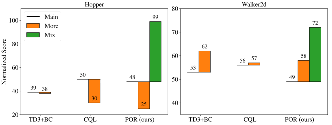
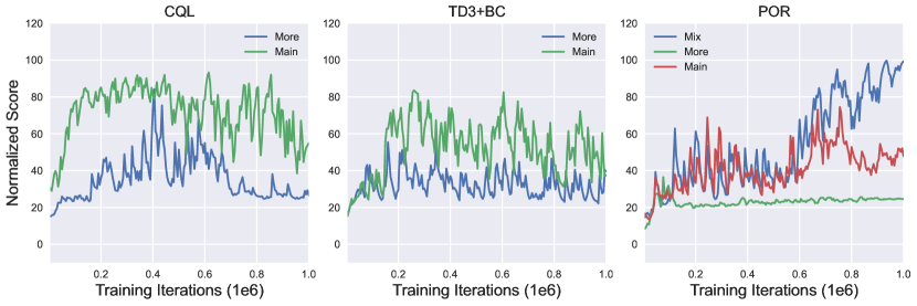
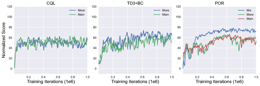
Naïvely, we can combine and as a new offline dataset , then run any off-the-shelf offline RL algorithm. We label this training scheme as "more". We also label the original training scheme that only uses as "main". We test these two training schemes on two state-of-the-art offline RL algorithms, TD3+BC and CQL. The results shown in Figure 3 indicate that both "main" and "more" are insufficient to learn a good policy, The reason why "main" fails is that the resulting policy may not be able to generalize due to the limited size. While "more" can generalize better than "main" due to access to a much larger dataset, the policy will be negatively impacted by the low-quality data in as both TD3+BC and CQL contain the behavior regularization term.
Due to the availability of decoupled training, POR is able to use a different training scheme, we can keep the execute-policy learned from unchanged but use the combination of and to re-train the guide-policy. Note that in this scheme, we allow the use of an action-free dataset , which often appears in real-world scenarios (i.e., video data and third-person demonstrations) [49]. The value function will be more accurate and better generalized when combining with to have a larger data coverage (see exploration in online RL as an example). We label this unique training procedure as "mix". It can be shown in Figure 3 that, by doing so, POR could have a super large improvement over "main" and "more". The version "mix" brings POR up to , close to the upper limit of the performance in the hopper environment, with only limited data. In the walker2d environment, POR with "mix" also outperforms all other baselines.
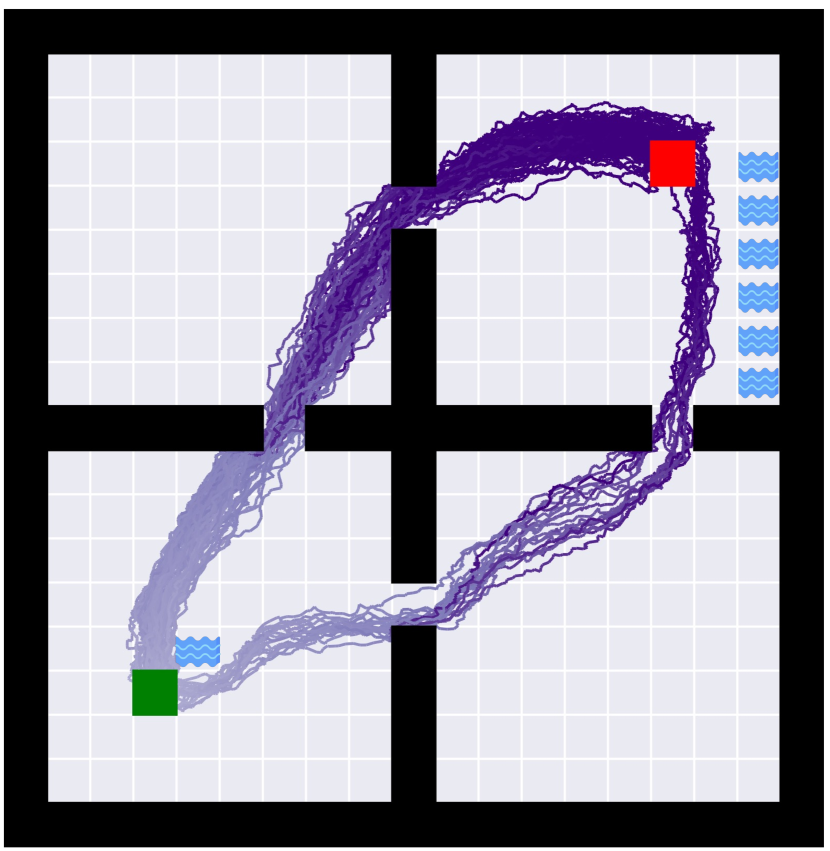
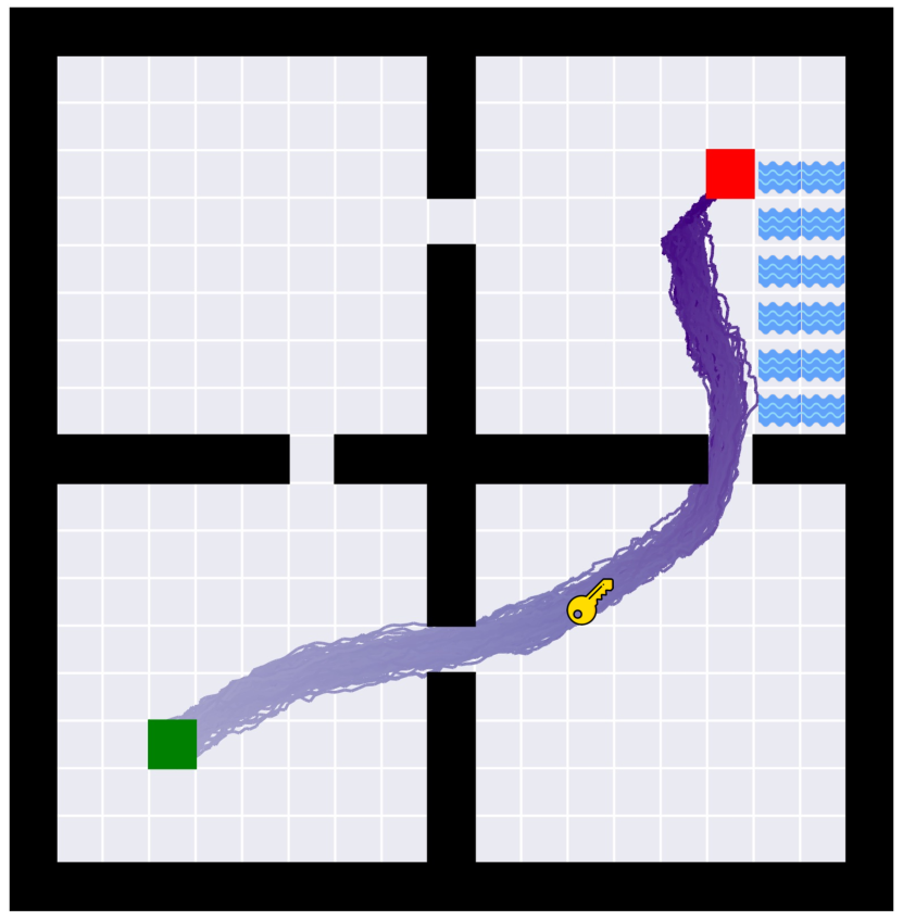
Change guide-policy in new tasks Then, we study whether we can use the guide-policy to do a lightweight adaptation to new tasks, without changing the execute-policy. We conduct experiments on the continuous variant of the classic four-room environment [20]. The training data consists of trajectories collected by a goal-reaching controller with the start and end locations sampled randomly at non-wall locations, mixed with data collected by a random policy. In this environment, we introduce three different tasks: Task A (Four-room) needs the agent to travel from the start location to the goal location, besides that, Task B (Four-room-river) and task C (Four-room-key) require the agent to bypass the river or get a key before arriving at the goal location.
We first train the guide-policy and the execute-policy to solve task A. In task B and task C, we re-train the guide-policy using the corresponding reward function in that task and reuse the execute-policy from Task A. In Figure 4, we can see that by doing so, POR is able to successfully solve task B and task C. In detail, in task B, POR is aware of the river and correctly bypasses it. In task C, POR only chooses to pass the bottom door, this is owing to the awareness of the importance of obtaining the key before reaching the goal. This result shows the strong adaptation ablity of the guide-policy for different tasks, as well as the generalization ability of the execute-policy across different tasks.
 to the goal
  . Besides, task B requires the agent not to fall into the river
  and task C requires the agent to get the key
  as well as avoiding the river
  before arriving at the goal location.
 6 Conclusions and Limitations
In this work, we propose a new offline RL paradigm, POR, which leverages the training stability of imitation-style methods while still encouraging logical out-of-distribution generalization. POR allows state-compositionality rather than action-compositionality from the dataset. Through theoretical analysis and extensive experiments, we show that POR outperforms prior methods on a variety of datasets, especially those with low quality. We also empirically demonstrate the additional benefits of POR in terms of improving with supplementary suboptimal data and easily adapting to new tasks. We hope that POR could shed light on how to enable state-compositionality in offline RL, which connects well to goal-conditioned RL and hierarchical RL [12]. One limitation of POR is that the prediction error of the guide-policy may be large when the state space is high-dimensional. However, this can be alleviated with the help of representation learning [31; 65].
Acknowledgments This work is supported by fundings from AsiaInfo. We thank Michael Janner for providing the code of the continuous four-room environment. We thank Junwu Xiong, James Zhang for their feedback on earlier versions of the manuscript.
References
- [1] Gaon An, Seungyong Moon, Jang-Hyun Kim, and Hyun Oh Song. Uncertainty-based offline reinforcement learning with diversified q-ensemble. Proc. of NeurIPS, 2021.
- [2] Jimmy Lei Ba, Jamie Ryan Kiros, and Geoffrey E Hinton. Layer normalization. ArXiv preprint, 2016.
- [3] Chenjia Bai, Lingxiao Wang, Zhuoran Yang, Zhi-Hong Deng, Animesh Garg, Peng Liu, and Zhaoran Wang. Pessimistic bootstrapping for uncertainty-driven offline reinforcement learning. In Proc. of ICLR, 2021.
- [4] David Brandfonbrener, Alberto Bietti, Jacob Buckman, Romain Laroche, and Joan Bruna. When does return-conditioned supervised learning work for offline reinforcement learning? In Proc. of NeurIPS, 2022.
- [5] David Brandfonbrener, William F Whitney, Rajesh Ranganath, and Joan Bruna. Offline rl without off-policy evaluation. Proc. of NeurIPS, 2021.
- [6] David Brandfonbrener, William F Whitney, Rajesh Ranganath, and Joan Bruna. Quantile filtered imitation learning. ArXiv preprint, 2021.
- [7] Lili Chen, Kevin Lu, Aravind Rajeswaran, Kimin Lee, Aditya Grover, Misha Laskin, Pieter Abbeel, Aravind Srinivas, and Igor Mordatch. Decision transformer: Reinforcement learning via sequence modeling. Proc. of NeurIPS, 2021.
- [8] Xinyue Chen, Zijian Zhou, Zheng Wang, Che Wang, Yanqiu Wu, and Keith W. Ross. BAIL: best-action imitation learning for batch deep reinforcement learning. In Proc. of NeurIPS, 2020.
- [9] Paul Christiano, Zain Shah, Igor Mordatch, Jonas Schneider, Trevor Blackwell, Joshua Tobin, Pieter Abbeel, and Wojciech Zaremba. Transfer from simulation to real world through learning deep inverse dynamics model. ArXiv preprint, 2016.
- [10] Scott Emmons, Benjamin Eysenbach, Ilya Kostrikov, and Sergey Levine. Rvs: What is essential for offline rl via supervised learning? ArXiv preprint, 2021.
- [11] Benjamin Eysenbach, Soumith Udatha, Sergey Levine, and Ruslan Salakhutdinov. Imitating past successes can be very suboptimal. In Proc. of NeurIPS, 2022.
- [12] Carlos Florensa, David Held, Xinyang Geng, and Pieter Abbeel. Automatic goal generation for reinforcement learning agents. In Proc. of ICML, 2018.
- [13] Justin Fu, Aviral Kumar, Ofir Nachum, George Tucker, and Sergey Levine. D4rl: Datasets for deep data-driven reinforcement learning. ArXiv preprint, 2020.
- [14] Scott Fujimoto and Shixiang Shane Gu. A minimalist approach to offline reinforcement learning. ArXiv preprint, 2021.
- [15] Scott Fujimoto, Herke van Hoof, and David Meger. Addressing function approximation error in actor-critic methods. In Proc. of ICML, pages 1582–1591, 2018.
- [16] Dibya Ghosh, Abhishek Gupta, Ashwin Reddy, Justin Fu, Coline Manon Devin, Benjamin Eysenbach, and Sergey Levine. Learning to reach goals via iterated supervised learning. In Proc. of ICLR, 2021.
- [17] Caglar Gulcehre, Sergio Gómez Colmenarejo, Ziyu Wang, Jakub Sygnowski, Thomas Paine, Konrad Zolna, Yutian Chen, Matthew Hoffman, Razvan Pascanu, and Nando de Freitas. Regularized behavior value estimation. ArXiv preprint, 2021.
- [18] Tuomas Haarnoja, Aurick Zhou, Pieter Abbeel, and Sergey Levine. Soft actor-critic: Off-policy maximum entropy deep reinforcement learning with a stochastic actor. In Proc. of ICML, pages 1856–1865, 2018.
- [19] Geoffrey E. Hinton and Sam T. Roweis. Stochastic neighbor embedding. In Proc. of NeurIPS, pages 833–840, 2002.
- [20] Michael Janner, Qiyang Li, and Sergey Levine. Offline reinforcement learning as one big sequence modeling problem. Proc. of NeurIPS, 2021.
- [21] Sham M. Kakade. A natural policy gradient. In Proc. of NeurIPS, pages 1531–1538, 2001.
- [22] Dmitry Kalashnikov, Jacob Varley, Yevgen Chebotar, Benjamin Swanson, Rico Jonschkowski, Chelsea Finn, Sergey Levine, and Karol Hausman. Mt-opt: Continuous multi-task robotic reinforcement learning at scale. ArXiv preprint, 2021.
- [23] Rahul Kidambi, Aravind Rajeswaran, Praneeth Netrapalli, and Thorsten Joachims. Morel: Model-based offline reinforcement learning. In Proc. of NeurIPS, 2020.
- [24] Diederik P. Kingma and Jimmy Ba. Adam: A method for stochastic optimization. In Proc. of ICLR, 2015.
- [25] Ilya Kostrikov, Rob Fergus, Jonathan Tompson, and Ofir Nachum. Offline reinforcement learning with fisher divergence critic regularization. In Proc. of ICML, pages 5774–5783, 2021.
- [26] Ilya Kostrikov, Ashvin Nair, and Sergey Levine. Offline reinforcement learning with implicit q-learning. ArXiv preprint, 2021.
- [27] Aviral Kumar, Justin Fu, Matthew Soh, George Tucker, and Sergey Levine. Stabilizing off-policy q-learning via bootstrapping error reduction. In Proc. of NeurIPS, pages 11761–11771, 2019.
- [28] Aviral Kumar, Xue Bin Peng, and Sergey Levine. Reward-conditioned policies. ArXiv preprint, 2019.
- [29] Aviral Kumar, Aurick Zhou, George Tucker, and Sergey Levine. Conservative q-learning for offline reinforcement learning. In Proc. of NeurIPS, 2020.
- [30] Sascha Lange, Thomas Gabel, and Martin Riedmiller. Batch reinforcement learning. In Reinforcement learning. 2012.
- [31] Michael Laskin, Aravind Srinivas, and Pieter Abbeel. CURL: contrastive unsupervised representations for reinforcement learning. In Proc. of ICML, pages 5639–5650, 2020.
- [32] Sergey Levine, Aviral Kumar, George Tucker, and Justin Fu. Offline reinforcement learning: Tutorial, review, and perspectives on open problems. ArXiv preprint, 2020.
- [33] Hsueh-Ti Derek Liu, Francis Williams, Alec Jacobson, Sanja Fidler, and Or Litany. Learning smooth neural functions via lipschitz regularization. ArXiv preprint, 2022.
- [34] Minghuan Liu, Zhengbang Zhu, Yuzheng Zhuang, Weinan Zhang, Jianye Hao, Yong Yu, and Jun Wang. Plan your target and learn your skills: Transferable state-only imitation learning via decoupled policy optimization. ArXiv preprint, 2022.
- [35] Corey Lynch, Mohi Khansari, Ted Xiao, Vikash Kumar, Jonathan Tompson, Sergey Levine, and Pierre Sermanet. Learning latent plans from play. In Conference on robot learning, 2020.
- [36] Xiaoteng Ma, Yiqin Yang, Hao Hu, Qihan Liu, Jun Yang, Chongjie Zhang, Qianchuan Zhao, and Bin Liang. Offline reinforcement learning with value-based episodic memory. In Proc. of ICLR, 2022.
- [37] Takeru Miyato, Toshiki Kataoka, Masanori Koyama, and Yuichi Yoshida. Spectral normalization for generative adversarial networks. In Proc. of ICLR, 2018.
- [38] Ofir Nachum, Bo Dai, Ilya Kostrikov, Yinlam Chow, Lihong Li, and Dale Schuurmans. Algaedice: Policy gradient from arbitrary experience. ArXiv preprint, 2019.
- [39] Ashvin Nair, Murtaza Dalal, Abhishek Gupta, and Sergey Levine. Accelerating online reinforcement learning with offline datasets. ArXiv preprint, 2020.
- [40] Deepak Pathak, Pulkit Agrawal, Alexei A. Efros, and Trevor Darrell. Curiosity-driven exploration by self-supervised prediction. In Proc. of ICML, pages 2778–2787, 2017.
- [41] Xue Bin Peng, Aviral Kumar, Grace Zhang, and Sergey Levine. Advantage-weighted regression: Simple and scalable off-policy reinforcement learning. ArXiv preprint, 2019.
- [42] Jan Peters and Stefan Schaal. Reinforcement learning by reward-weighted regression for operational space control. In Proc. of ICML, 2007.
- [43] Dean A Pomerleau. Alvinn: An autonomous land vehicle in a neural network. In Proc. of NeurIPS, 1989.
- [44] John Schulman, Sergey Levine, Pieter Abbeel, Michael I. Jordan, and Philipp Moritz. Trust region policy optimization. In Proc. of ICML, pages 1889–1897, 2015.
- [45] David Silver, Guy Lever, Nicolas Heess, Thomas Degris, Daan Wierstra, and Martin A. Riedmiller. Deterministic policy gradient algorithms. In Proc. of ICML, pages 387–395, 2014.
- [46] Rupesh Kumar Srivastava, Pranav Shyam, Filipe Mutz, Wojciech Jaśkowski, and Jürgen Schmidhuber. Training agents using upside-down reinforcement learning. ArXiv preprint, 2019.
- [47] Richard S Sutton, Andrew G Barto, et al. Introduction to reinforcement learning. MIT press Cambridge, 1998.
- [48] Shengpu Tang and Jenna Wiens. Model selection for offline reinforcement learning: Practical considerations for healthcare settings. In Proc. of ML4H, 2021.
- [49] Faraz Torabi, Garrett Warnell, and Peter Stone. Behavioral cloning from observation. In Proc. of IJCAI, pages 4950–4957, 2018.
- [50] Hado Van Hasselt, Yotam Doron, Florian Strub, Matteo Hessel, Nicolas Sonnerat, and Joseph Modayil. Deep reinforcement learning and the deadly triad. ArXiv preprint, 2018.
- [51] Aladin Virmaux and Kevin Scaman. Lipschitz regularity of deep neural networks: analysis and efficient estimation. In Proc. of NeurIPS, pages 3839–3848, 2018.
- [52] Ziyu Wang, Alexander Novikov, Konrad Zolna, Josh Merel, Jost Tobias Springenberg, Scott E. Reed, Bobak Shahriari, Noah Y. Siegel, Çaglar Gülçehre, Nicolas Heess, and Nando de Freitas. Critic regularized regression. In Proc. of NeurIPS, 2020.
- [53] Christopher JCH Watkins and Peter Dayan. Q-learning. Machine learning, 1992.
- [54] Yifan Wu, George Tucker, and Ofir Nachum. Behavior regularized offline reinforcement learning. ArXiv preprint, 2019.
- [55] Yue Wu, Shuangfei Zhai, Nitish Srivastava, Joshua M. Susskind, Jian Zhang, Ruslan Salakhutdinov, and Hanlin Goh. Uncertainty weighted actor-critic for offline reinforcement learning. In Proc. of ICML, pages 11319–11328, 2021.
- [56] Haoran Xu, Li Jiang, Jianxiong Li, Zhuoran Yang, Zhaoran Wang, Victor Wai Kin Chan, and Xianyuan Zhan. Offline rl with no ood actions: In-sample learning via implicit value regularization. In Proc. of ICLR, 2023.
- [57] Haoran Xu, Xianyuan Zhan, Jianxiong Li, and Honglei Yin. Offline reinforcement learning with soft behavior regularization. ArXiv preprint, 2021.
- [58] Haoran Xu, Xianyuan Zhan, Honglei Yin, and Huiling Qin. Discriminator-weighted offline imitation learning from suboptimal demonstrations. In Proc. of ICML, pages 24725–24742, 2022.
- [59] Haoran Xu, Xianyuan Zhan, and Xiangyu Zhu. Constraints penalized q-learning for safe offline reinforcement learning. In Proc. of AAAI, pages 8753–8760, 2022.
- [60] Rui Yang, Yiming Lu, Wenzhe Li, Hao Sun, Meng Fang, Yali Du, Xiu Li, Lei Han, and Chongjie Zhang. Rethinking goal-conditioned supervised learning and its connection to offline rl. ArXiv preprint, 2022.
- [61] Tianhe Yu, Aviral Kumar, Yevgen Chebotar, Karol Hausman, Chelsea Finn, and Sergey Levine. How to leverage unlabeled data in offline reinforcement learning. ArXiv preprint, 2022.
- [62] Tianhe Yu, Garrett Thomas, Lantao Yu, Stefano Ermon, James Y. Zou, Sergey Levine, Chelsea Finn, and Tengyu Ma. MOPO: model-based offline policy optimization. In Proc. of NeurIPS, 2020.
- [63] Xianyuan Zhan, Haoran Xu, Yue Zhang, Xiangyu Zhu, Honglei Yin, and Yu Zheng. Deepthermal: Combustion optimization for thermal power generating units using offline reinforcement learning. In Proc. of AAAI, pages 4680–4688, 2022.
- [64] Xianyuan Zhan, Xiangyu Zhu, and Haoran Xu. Model-based offline planning with trajectory pruning. In Proc. of IJCAI, 2022.
- [65] Amy Zhang, Rowan Thomas McAllister, Roberto Calandra, Yarin Gal, and Sergey Levine. Learning invariant representations for reinforcement learning without reconstruction. In Proc. of ICLR, 2021.
- [66] Wenxuan Zhou, Sujay Bajracharya, and David Held. Latent action space for offline reinforcement learning. In Conference on Robot Learning, 2020.
Checklist
-
1.
For all authors…
-
(a)
Do the main claims made in the abstract and introduction accurately reflect the paper’s contributions and scope? [Yes]
-
(b)
Did you describe the limitations of your work? [Yes] See Section 6.
-
(c)
Did you discuss any potential negative societal impacts of your work? [Yes] See Section 6.
-
(d)
Have you read the ethics review guidelines and ensured that your paper conforms to them? [Yes]
-
(a)
- 2.
-
3.
If you ran experiments…
-
(a)
Did you include the code, data, and instructions needed to reproduce the main experimental results (either in the supplemental material or as a URL)? [Yes] See the supplement material.
-
(b)
Did you specify all the training details (e.g., data splits, hyperparameters, how they were chosen)? [Yes] See Appendix D.
-
(c)
Did you report error bars (e.g., with respect to the random seed after running experiments multiple times)? [Yes] In all related figures.
-
(d)
Did you include the total amount of computing and the type of resources used (e.g., type of GPUs, internal cluster, or cloud provider)? [Yes] See Appendix D.
-
(a)
-
4.
If you are using existing assets (e.g., code, data, models) or curating/releasing new assets…
-
(a)
If your work uses existing assets, did you cite the creators? [Yes] Data is from [13].
-
(b)
Did you mention the license of the assets? [Yes] The license is Apache 2.0.
-
(c)
Did you include any new assets either in the supplemental material or as a URL? [Yes] See supplement for code and four room dataset.
-
(d)
Did you discuss whether and how consent was obtained from people whose data you’re using/curating? [N/A] Data is simulated.
-
(e)
Did you discuss whether the data you are using/curating contains personally identifiable information or offensive content? [N/A] Data is simulated.
-
(a)
-
5.
If you used crowdsourcing or conducted research with human subjects…
-
(a)
Did you include the full text of instructions given to participants and screenshots, if applicable? [N/A]
-
(b)
Did you describe any potential participant risks, with links to Institutional Review Board (IRB) approvals, if applicable? [N/A]
-
(c)
Did you include the estimated hourly wage paid to participants and the total amount spent on participant compensation? [N/A]
-
(a)
Appendix A More Discussion
Why One-step and IQL are imitation-based methods? The core difference between RL-based and imitation-based methods is that RL-based methods learn a value function of policy while imitation-based methods don’t. Learning the value function of requires off-policy evaluation of (i.e., learning or ), which is prone to distribution shift. The policy evaluation and policy improvement will also affect each other as they are coupled.
Imitation-based methods don’t learn or , but some of them do learn a value function. We call these methods imitation-based because they learn the value function using only dataset samples, the value function actually tells how advantageous it could be under the behavior policy, much like imitation learning. Also, the policy learning objective of One-step (with exponentially-weighted improvement operator) and IQL can be written as , which uses dataset actions to doing behavior cloning with different weights (One-step and IQL learn different value functions).
Cloning dataset actions can only do action-stitching, which loses the ability to surpass the dataset by out-of-distribution (action) generalization. For example, in our toy example in Section 4.1, action-stitching methods at most learn the shortest path that contained in the datset. This is suboptimal especially when there does not exist one complete path starting from the start location to the goal location in the offline dataset.
How can we do beyond action-stitching? One way is to use RL-based methods, by querying an accurate , we can get a different-yet-optimal action , but is hard to estimate. Another way is like what POR did, we learn an out-of-distribution state indicator, i.e., the guide-policy , to guide the policy to the optimal next state. If the execute-policy can generalize well, it will also output a different yet optimal action .
Appendix B More Related Work
Our work decouples the state-to-action policy into two modules, i.e., the guide-policy and the execute-policy. The execute-policy is actually an inverse dynamics model, which has been widely used in various ways in sequential decision-making. In exploration, inverse dynamics can be used to learn representations of the controllable aspects of the state [40]. In imitation learning, [49] and [34] train an inverse dynamics model to label the state-only demonstrations with inferred actions. [9] use inverse dynamics models to translate actions taken in a simulated environment to the real world.
Recently, there has been an emergence of work [46, 16] highlighting the connection of imitation learning and reinforcement learning. Specifically, rather than learn to map states and actions to reward, as is typical in reinforcement learning, [46] trains a model to predict actions given a state and an outcome, which could be the amount of reward the agent is to collect within a certain amount of time. [16] uses a similar idea, predicting actions conditioned on an initial state, a goal state, and the amount of time left to achieve the goal. These methods are perhaps the closest work to our algorithm, however, we study the offline setting and motivate the usage of an inverse dynamics model from a different perspective (i.e., state-stitching).
Appendix C Proof
In this section, we provide the proof of Theorem 1.
Proof.
Appendix D Experimental Details
In this section, we provide the experimental details of our paper.
D.1 D4RL Experiments
Data collection The datasets in D4RL have been generated as follows: random: roll out a randomly initialized policy for 1M steps. expert: 1M samples from a policy trained to completion with SAC [18]. medium: 1M samples from a policy trained to approximately 1/3 the performance of the expert. medium-replay: replay buffer of a policy trained up to the performance of the medium agent. medium-expert: 50-50 split of medium and expert data. For all datasets we use the v2 version.
Implementation details Our implementation of 10%BC is as follows, we first filter the top 10 trajectories in terms of the trajectory return, and then run behaviour cloning on those filtered data. The hyperparameters of POR are present in Table LABEL:table:_hyperparams and LABEL:table:_hyperparams_more. We use target networks for the -function and use clipped double -learning (take the minimum of two -functions) for all updates. In some MuJoCo tasks, we add Layer Normalization [2] to -networks to help stabilize training.
| Hyperparameter | Value | |
| Architecture | Value network hidden dim | 256 |
| Value network hidden layers | 2 | |
| Value network activation function | ReLU | |
| Guide-policy hidden dim | 256 | |
| Guide-policy hidden layers | 2 | |
| Guide-policy activation function | ReLU | |
| Execute-policy hidden dim | 1024 | |
| Execute-policy hidden layers | 2 | |
| Execute-policy activation function | ReLU | |
| Hyperparameters | Optimizer | Adam [24] |
| Value netowrk learning rate | 1e-4 | |
| Target Value netowrk moving average | 0.05 | |
| Mini-batch size | 256 | |
| Discount factor | 0.99 | |
| Normalize | False |
| Env | Guide-policy learning objective | Policy learning rate | ||
| antmaze-umaze-v2 | (6) | 0.9 | 10.0 | 1e-3 |
| antmaze-umaze-diverse-v2 | (6) | 0.9 | 10.0 | 1e-3 |
| antmaze-medium-play-v2 | (6) | 0.9 | 10.0 | 1e-4 |
| antmaze-medium-diverse-v2 | (6) | 0.9 | 10.0 | 1e-4 |
| antmaze-large-play-v2 | (6) | 0.9 | 10.0 | 1e-4 |
| antmaze-large-diverse-v2 | (6) | 0.9 | 10.0 | 1e-4 |
| halfcheetah-medium-v2 | (6) | 0.5 | 3.0 | 1e-3 |
| hopper-medium-v2 | (5) | 0.7 | 50.0 | 1e-3 |
| walker2d-medium-v2 | (6) | 0.5 | 3.0 | 1e-3 |
| halfcheetah-medium-replay-v2 | (6) | 0.5 | 3.0 | 1e-3 |
| hopper-medium-replay-v2 | (5) | 0.7 | 50.0 | 1e-3 |
| walker2d-medium-replay-v2 | (6) | 0.5 | 3.0 | 1e-3 |
| halfcheetah-medium-expert-v2 | (6) | 0.5 | 3.0 | 1e-3 |
| hopper-medium-expert-v2 | (5) | 0.7 | 5.0 | 1e-3 |
| walker2d-medium-expert-v2 | (6) | 0.5 | 3.0 | 1e-3 |
| Env | Guide-policy learning objective | Policy learning rate | ||
| antmaze-umaze-v2 | (6) | 1.0 | 10.0 | 1e-3 |
| antmaze-umaze-diverse-v2 | (6) | 0.5 | 10.0 | 1e-3 |
| antmaze-medium-play-v2 | (6) | 0.1 | 10.0 | 1e-4 |
| antmaze-medium-diverse-v2 | (6) | 0.1 | 10.0 | 1e-4 |
| antmaze-large-play-v2 | (6) | 0.1 | 10.0 | 1e-4 |
| antmaze-large-diverse-v2 | (6) | 0.3 | 10.0 | 1e-4 |
D.2 Additional Suboptimal Data Experiments
Data collection and settings
In this experiment, we use different part of medium-replay datasets as and . More specific, we use to transitions to constitute and use to transitions to constitute .
Implementation details We use the same hyperparamters of POR, shown in Table LABEL:table:_hyperparams. Our implementations of TD3+BC†††https://github.com/sfujim/TD3_BC [15], CQL‡‡‡https://github.com/aviralkumar2907/CQL [29] is from the author-provided implenmentation from Github, and we keep all parameters the same to the author-provided implementation.
| Hyperparameter | Value | |
| Architecture | Critic hidden dim | 256 |
| Critic hidden layers | 3 | |
| Critic activation function | ReLU | |
| Actor hidden dim | 256 | |
| Actor hidden layers | 3 | |
| Actor activation function | ReLU | |
| CQL Hyperparameters | Optimizer | Adam [24] |
| Critic learning rate | 3e-4 | |
| Actor learning rate | 1e-4 | |
| Mini-batch size | 256 | |
| Discount factor | 0.99 | |
| Target update rate | 5e-3 | |
| Target entropy | -1 Action Dim | |
| Entropy in Q target | True | |
| Lagrange | False | |
| Num sampled actions (during eval) | 10 | |
| Num sampled actions (logsumexp) | 10 | |
| 10 |
| Hyperparameter | Value | |
| Architecture | Critic hidden dim | 256 |
| Critic hidden layers | 2 | |
| Critic activation function | ReLU | |
| Actor hidden dim | 256 | |
| Actor hidden layers | 2 | |
| Actor activation function | ReLU | |
| TD3+BC Hyperparameters | Optimizer | Adam [24] |
| Critic learning rate | 3e-4 | |
| Actor learning rate | 3e-4 | |
| Mini-batch size | 256 | |
| Discount factor | 0.99 | |
| Target update rate | 5e-3 | |
| Policy noise | 0.2 | |
| Policy noise clipping | (-0.5, 0.5) | |
| Policy update frequency | 2 | |
| 2.5 |
D.3 Four-room Experiments
Environment settings We use the continuous variant of the classic four-room environment from [20]. This continuous variant of four-rooms is basically the same as the traditional classic four-room environment in the environment design. There are grids that consist of four rooms with only one block channel with neighboring rooms. The goal of this environment is to make the agent travel from one location to another different location. Those tasks are challenging as their reward is extremely spare, they need the agent to have the ability to explore efficiently through the whole state space. The action and observation space are shown in Table 8. The first and second dimension of the action space represents the distance to travel on the -axis and -axis, respectively. The first and second dimension of the observation space represents the coordinate on the -axis and -axis, respectively.
| Action space | Box(-0.1, 0.1, (2,), float32) |
| Observation space | Box(-18, 18, (2,), float32) |
| Action dimension | 2 |
| Observation dimension | 2 |
In task A (Four-room), only reaching the goal will give the agent a reward of , otherwise the agent will get reward. When the agent reaches the target or the agent takes over 500 steps, the environment will terminate. In task B (Four-room-river), the agent will receive reward if it falls into the river, and the environment will be terminated. Also, the agent will get reward only when it reaches the goal. In task C (Four-room-key), the agent gets reward only when it reaches the goal and gets the key. Falling into the river will also give the agent reward.
Data collection and implementation details The training data consists of trajectories collected by a goal-reaching controller with the start and end locations sampled randomly at non-wall locations. To make the data more diverse, we also add trajectories from a random policy. We collect 100,000 transitions for each task. Figure LABEL:table:_four-room_hyperparamters shows the training hyperparameters of POR in the three four-room environments.
| Hyperparameter | Value | |
| Architecture | Value network hidden dim | 64 |
| Value network hidden layers | 2 | |
| Value network activation function | ReLU | |
| Guide-policy hidden dim | 64 | |
| Guide-policy hidden layers | 2 | |
| Guide-policy activation function | ReLU | |
| Execute-policy hidden dim | 64 | |
| Execute-policy hidden layers | 2 | |
| Execute-policy activation function | ReLU | |
| Training Hyperparameters | Optimizer | Adam [24] |
| Value network learning rate | 1e-4 | |
| Target V moving average | 0.05 | |
| Guide-policy learning rate | 1e-4 | |
| Execute-policy learning rate | 1e-4 | |
| Mini-batch size | 256 | |
| Discount factor | 0.99 | |
| Normalize | False | |
| Guide-policy learning objective | (6) | |
| 0.9 | ||
| 10.0 |
Appendix E Learning Curves
In this section, we provide the learning curves of our experiments in the main paper.
Appendix F Ablation Study on the Execute-Policy
We also present an ablation study on the execute-policy, with the aim to answer the following two questions: 1) How does network capacity affect the performance of the execute-policy? 2) How does the performance change if we use partial "good" data, instead of full data, to train the execute policy?
To answer the first question, we compare two choices of network size: a big network with hidden units and a small network with hidden units. To answer the second question, we compare with the choice that only selects a subset of the dataset to train the execute policy. Concretely, we choose the top trajectories in the dataset, ordered by episode returns. We sweep over and choose the best score. We give the mean scores of AntMaze (A) and MuJoCo (M) datasets in Table 10. It can be seen that adopting a big network consistently gives a better performance, which is also found in [10]. Using partial data will result in a less-performed policy, especially on AntMaze datasets. Note that in MuJoCo datasets, the performance didn’t drop too much. This is because MuJoCo datasets don’t require the compositionality ability, using partial trajectories could already achieve high scores.
| Big Network | Small Network | |
| Full | A: 76.2, M: 65.7 | A: 63.8, M: 57.0 |
| Partial | A: 52.4, M: 60.9 | A: 41.5, M: 56.7 |