FedCross: Towards Accurate Federated Learning via Multi-Model Cross Aggregation

Abstract.

Due to the remarkable performance in preserving data privacy for decentralized data scenarios, Federated Learning (FL) has been considered as a promising distributed machine learning paradigm to deal with data silos problems. Typically, conventional FL approaches adopts a one-to-multi training scheme, where the cloud server keeps only one single global model for all the involved clients for the purpose of model aggregation. However, this scheme suffers from inferior classification performance, since only one global model cannot always accommodate all the incompatible convergence directions of local models, resulting in low convergence rate and classification accuracy. To address this issue, this paper presents an efficient FL framework named FedCross, which adopts a novel multi-to-multi FL training scheme based on our proposed similarity-based multi-model cross aggregation method. Unlike traditional FL methods, in each round of FL training, FedCross uses a small set of distinct intermediate models to conduct weighted fusion under the guidance of model similarities. In this way, the intermediate models used by FedCross can sufficiently respect the convergence characteristics of clients, thus leading to much fewer conflicts in tuning the convergence directions of clients. Finally, in the deployment stage, FedCross forms a global model for all the clients by performing the federated averaging on the trained immediate models. Experimental results on three well-known datasets demonstrate that, compared with state-of-the-art FL approaches, FedCross can significantly improve FL accuracy in both IID and non-IID scenarios without causing additional communication overhead.

1. Introduction

Although artificial intelligence (AI) methods have shown advantages in handling more and more complex tasks, traditional centralized AI approaches cannot handle Internet of Things (IoT) or mobile edge computing (MEC) scenarios due to the limitation of data privacy and decentralization. As a popular privacy-preserving and distributed AI paradigm, Federated learning (FL) (McMahan et al., 2017; Yang et al., 2019; Zhang et al., 2020; Yang et al., 2021; Zhang et al., 2021; Wu et al., 2021) is promising to become the infrastructure for AI applications in IoT (Zhang et al., 2020; Lim et al., 2021; Uddin et al., 2020; Li et al., 2021b; Cui et al., 2021; Rey et al., 2022) and MEC (Liu et al., 2022; Luo et al., 2021b; Yang et al., 2021; Wu et al., 2020; Li et al., 2021a) scenarios. By dispatching a global model to multiple clients for local training and then aggregating the trained models, FL realizes distributed model training without data sharing, which also greatly reduces the risk of data privacy leakage.

However, the traditional one-to-multi allocation way, namely dispatch many copies of the global model to local clients, inevitably encounters the problem of gradient divergence (Kairouz et al., 2021; Zhuang et al., 2020). Things become even worse when local optimization directions are widely divergent due to the non-IID (Wang et al., 2020; Li et al., 2022; Luo et al., 2021a; Li and Zhan, 2021) data distribution among local clients. This is because the non-IID data will lead to a larger difference in the local optimization direction between clients. To alleviate the gradient divergence and improve the accuracy of the federated learning model, the existing FL methods mainly focus on three handling means, i.e., global control variable-based methods (Karimireddy et al., 2020; Huang et al., 2021), knowledge distillation-based methods (Zhang et al., 2022; Lin et al., 2020; Ozkara et al., 2021), and client clustering-based methods (Chen et al., 2020; Fraboni et al., 2021), respectively. The basic idea of them is to alleviate gradient divergence by constraining the direction of local training or adjusting the weight of aggregation.

However, in our speculation, the main factor that limits the performance of FL method is the one-to-multi architecture, which has not been considered by previous methods yet. In each training round, the optimization direction of each local client is divergent, leading to the different update status of key parameters in each local model. In the one-to-multi architecture, it is difficult for the global model to accurately retain the key parameters of all the local model, which inevitably lead to information loss. The coarse-grained aggregation method of traditional one-to-multi framework greatly limits the performance of the global model. Therefore, how to construct a fine-grained distributed model training&aggregation method is worthy of research.

To address the above challenge, this paper presents a novel FL framework named FedCross, which adopts our proposed weighted fusion-based training scheme with intermediate models in a multi-to-multi manner. In specific, FedCross dispatches multiple isomorphism middleware models to multiple clients at each FL training round. Instead of using multi-to-one aggregation in the training procedure, FedCross adopts a multi-model cross-aggregation strategy, which updates each middleware model (host model) by aggregating it with its collaborative model (guest model). In addition, the cross-aggregation adopts a non-average aggregation mechanism, where the host model will get a higher weight in the aggregation. Through cross-aggregation, each middleware model can learn knowledge from the collaborative model with less damage to its own knowledge as much as possible. By dispatching these updated middleware models to clients for local training, FedCross achieves multi-to-multi FL training. The global model is generated at the deployment procedure by average aggregating all the middleware models. Through the cross-aggregation and continuous training of middleware models, the discrete knowledge between middleware models will gradually become unified. Compared with aggregating all the models with one global model, this unification process is more gentle and reasonable, leading to great alleviation of the gradient divergence problem. In summary, this paper presents the following three major contributions:

• We present a novel multi-to-multi FL framework named FedCross, which creatively adds multiple only-for-training middleware models to alleviate the gradient divergence problem in model aggregation and generates the only-for-deployment global model by aggregating middleware models.

• We present a novel multi-model cross-aggregation algorithm, which matches each middleware model with a collaborative model by a model selection strategy and fuses them according to a certain weight to achieve gentle knowledge sharing.

• We conduct extensive experiments to evaluate the performance and pervasiveness of FedCross and explore proper configuration of FedCross in both IID and non-IID scenarios.

The rest of this paper is organized as follows. Section 2 presents the preliminaries of federated learning and introduces various kinds of FL optimization methods. Section 3 details the implementation of our proposed FedCross approach. Section 4 performs the comparison between our FedCross and state-of-the-art FL methods. Finally, Section 5 concludes the paper.

2. Backgrounds and Related Work

2.1. Backgrounds of Federated Learning

The traditional one-to-multi FL consists of a central cloud for the aggregation of local models and multiple clients for local model training. To train a global model with good performance on all clients, each FL model training round consists of four main steps: i) model dispatching where the cloud server dispatches the global model to clients for model training; ii) local training where clients train dispatched models with their own data; iii) local model upload where clients upload trained local model to the cloud server; iv) model aggregation where the cloud server aggregates all the uploaded local models to generate a new global model. The most classic model aggregation is the averaging aggregation from FedAvg (McMahan et al., 2017), which is defined as follows:

(1) $$\begin{split}&\min_{w}F(w)=\frac{1}{N}\sum_{i=1}^{N}f_{i}(w),\\ \ s.t.,&\ f_{i}(w)=\frac{1}{n_{i}}\sum_{j=1}^{n_{i}}\ell(w;s_{j};l_{j}),\end{split}$$

where $N$ denotes the number of clients, $n_{i}$ indicates the number of data samples in the $i^{th}$ client, $\ell$ indicates a loss function (e.g., cross-entropy loss), $s_{j}$ indicates a sample, and $l_{j}$ is the label of $s_{j}$.

2.2. Related Work for FL Optimization

Although the traditional one-to-multi FL can achieve distributed model training for clients without data sharing, its performance is still severely limited by its coarse-grained aggregation. To deal with this challenge, many optimization approaches have been proposed to improve the performance of FL based on FedAvg. According to our knowledge, these optimization methods mainly from three perspectives, i.e., global control variable, client grouping, and knowledge distillation.

The global control variable-based methods attempts to use a global variable to guide the training direction of local training, thereby alleviating gradient divergence. For example, SCAFFOLD (Karimireddy et al., 2020) dispatches global control variables to clients to correct the “client-drift” problem in the local training process. FedProx (Li et al., 2020) regularizes local loss functions with a proximal term to stabilize the model convergence, where the proximal term is the squared distance between the local models and the global model.

The client grouping-based methods try to group the clients based on the similarity of their data distribution and select clients to participate in training based on groups. However, since the client data distribution cannot be obtained directly, the existing methods group clients through easily obtainable information such as model similarity. For example, FedCluster (Chen et al., 2020) groups the clients into multiple clusters that perform federated learning cyclically in each learning round. CluSamp (Fraboni et al., 2021) uses either sample size or model similarity to group clients, which can reduce the variance of client stochastic aggregation parameters in FL.

The Knowledge Distillation (KD)-based methods uses a “teacher model” to guide the training of “student models”. In specific, the “student models” use the soft labels of the teacher model to perform model training, which can learn the knowledge of the teacher model. For example, FedAUX (Sattler et al., 2021) performs data-dependent distillation by using an auxiliary dataset to initialize the server model. FedGen (Zhu et al., 2021) performs data-free distillation and leverages a proxy dataset to address the heterogeneous FL problem using a built-in generator. FedDF (Lin et al., 2020) uses ensemble distillation to accelerate by training the global model through unlabeled data on the outputs of local models.

Although the above approaches can improve FL performance from different perspectives, it still faces two problems. The first problem is additional non-negligible communication overheads. Since FL is often deployed in uncertain network quality, the increase in communication overhead will seriously affect the efficiency of FL. The second problem is the risk of data privacy exposure. Any attempt to obtain any information on the client (including data distribution, the similarity between clients, etc.) may increase the risk of privacy exposure. Furthermore, all these methods are based on the traditional one-to-multi approach, which is still strongly limited by the coarse-grained model aggregation. Different from the above FL optimization methods, FedCross presents a novel multi-to-multi framework to conduct a fine-grained model aggregation.

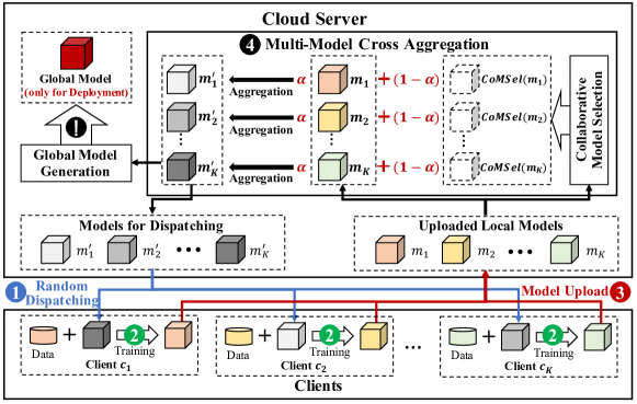
Figure 1. Framework and workflow of FedCross.

3. Our FedCross Approach

3.1. Overview of FedCross

The architecture of FedCross consists of a central cloud server and multiple local devices, which is the same as conventional one-to-multi FL frameworks. The main difference is that FedCross uses a multi-to-multi training and aggregation mechanism. In specific, FedCross uses multiple isomorphic middleware models for local training and updates these middleware models by a cross-aggregation strategy. FedCross still generates a global model, but the global model is only for deployment rather than model training. Figure 1 presents the framework and workflow of FedCross, which shows all the above two processes, i.e., model training and global model generation. The model training process trains middleware models, which involves 4 steps:

• Step 1 (Middleware Model Dispatching): The cloud server randomly dispatches $K$ middleware models to $K$ local clients. Note that each client receives a unique middleware model.

• Step 2 (Middleware Model Training): Clients train their received middleware model independently with local data.

• Step 3 (Model Upload): Uploading all the middleware models from clients to the cloud server.

• Step 4 (Multi-Model Cross Aggregation): For each middleware model $m_{i}$ ($1\leq i\leq K$), our method choose a collaborative model $m_{j}$ ($j\neq i$) as a complement. By aggregating each middleware model and its collaborative model with weights of $\alpha$ and $1-\alpha$, the cloud server can generate $K$ new middleware models (i.e., $m^{\prime}_{1},...,m^{\prime}_{K}$) for next round training.

The global model generation process aggregates multiple trained middleware models to generate a global model. Since in FedCross the global model is only used for model deployment, the global model generation and model training processes are asynchronous.

3.2. FedCross Implementation

Algorithm 1 presents the implementation of our FedCross approach. In each training round, FedCross selects $K$ clients to participate in model training. Line 1 initializes the $K$ dispatched models, where $W$ indicates the list of dispatched models. Line 1-1 present the model training process. Line 1 randomly selects $K$ clients for each round model training, where $L_{c}$ is the list of selected clients. Line 1 shuffles the order of the selected models, with which each dispatched model is given an equal chance to be trained by the client. Note that, without shuffling, each middleware model will be dispatched to the clients encountered in previous training rounds at a high probability. Line 1-1 dispatch models to according clients and conducts local training process. In Line 1 each client trains the received model using local data and uploads retrained local model to the cloud server. In Line 1, the cloud server updates the model list $W$ using the received trained model. Line 1 selects a collaborate model for each uploaded model. Line 1 aggregates each uploaded model with its collaborate model to generate $K$ models and Line 1 updates dispatched model list $W$ using these generated models. Line 1 generates a global model for deployment by aggregating all the models in $W$. Note that, since the global model does not participate in model training, global model generation can be performed asynchronously at any time point.

Input: i) $round$, # of training rounds;

ii) $C$, the set of clients;

iii) $K$, # of clients participating in each FL round.

Output: $w_{g}$, the global model.

1 FedCross($round$,$C$,$K$) begin

2       $W\leftarrow[w^{1}_{0},w^{2}_{0},...,w^{K}_{0}]\ \ \$ // initialize model list ;

3       for $r$ = 0, …, $round-1$ do

4             $L_{c}\leftarrow$ Random select $K$ clients from $C$;

5             $L_{c}\leftarrow Shuffle(L_{c})$;

6             /*parallel block*/

7             for $i$ = 1, …, $K$ do

8                   $v_{r+1}^{i}\leftarrow$LocalTraining$(w^{i}_{r},L_{c}[i])$;

9                   $W[i]\leftarrow v_{r+1}^{i}$;

10                  

11             end for

12             for $i$ = 1, …, $K$ do

13                   $v_{co}^{i}\leftarrow$CoModelSel$(v^{i}_{r+1},W)$;

14                   $w_{r+1}^{i}\leftarrow$CrossAggr$(v^{i}_{r+1},v_{co}^{i})$;

15                  

16             end for

17            $W\leftarrow[w_{r+1}^{1},w_{r+1}^{2},...,w_{r+1}^{K}]$;

18            

19       end for

20       $w_{g}\leftarrow$GlobalModelGen$(W)$;

21       return $w_{g}$;

22      

23 end

24

Algorithm 1 Implementation of FedCross

3.2.1. Collaborative Model Selection (CoModelSel)

FedCross selects a collaborative model for each model in the uploaded model list. Obviously, the selection criteria of the collaborative model is an interesting issue worth discussing. To explore the collaboration criteria, a reasonable and logical idea is to design selection criteria according to model characteristics. Thus we propose three kinds of different model selection criteria for various purposes: (1) adequacy and diversity of participation, (2) minimizing gradient divergence, (3) maximizing knowledge acquisition. Many strategies can be derived from these three criteria, and the strategy follows different criteria leading to various aggregation properties.

To fully exploit the information in uploaded models, the adequacy & diversity criteria encourages each model to participate in the updating of other models as much as possible. To be specific, a strategy (in order) that satisfies the adequacy & diversity criteria is in order collaboration. To ease model training, the gradient divergence minimization criteria encourage each model to find collaboration models which can facilitate convergence. To be specific, a strategy (highest similarity) that satisfies the gradient divergence minimization criteria is selecting the most similar model for the target model. The knowledge maximization criteria encourage each model to obtain more knowledge at each training round. To be specific, a strategy (lowest similarity) that satisfies the knowledge maximization criteria is selecting the least similar model for the target model. The detail of the three model selection strategies (i.e., in order, highest similarity, lowest similarity) is as follows:

In Order: For the $i^{th}$ model, the cloud server selects the $((i+(r\%(K-1)+1))\%K)^{th}$ model as the collaborative model in the $r^{th}$ training round. The detail of in order strategy is as follows

(2) $$CoModelSel(v^{i}_{r},W)=W[(i+(r\%(K-1)+1))\%K],$$

where $W$ is the list of uploaded local model parameters, $K$ is the number of uploaded models. Within this strategy, all the upload models are chosen to be collaborative models once in each round. Furthermore, after every $K-1$ training round, each model has collaborated once with all the other $K-1$ models.

The highest similarity: By calculating the model similarity between the uploaded models, each model aggregates the model with the highest similarity as follows:

(3) $$CoModelSel(v^{i}_{r},W)=\underset{v\in W\setminus\{v^{i}_{r}\}}{\arg\max}\ Similarity(v^{i}_{r},v),$$

where $W$ is the list of uploaded local model parameters and Similarity is a function to calculate model similarity. Note that the higher Similarity value means a higher similarity between the two models.

The lowest similarity: According to the formula of highest similarity strategy, the lowest similarity strategy encourages each model to select the model with the least similarity as the collaborative model:

(4) $$CoModelSel(v^{i}_{r},W)=\underset{v\in W\setminus\{v^{i}_{r}\}}{\arg\min}\ Similarity(v^{i}_{r},v)$$

The calculation method of model similarity are various according to the specific scene, for example, Eucledian Distance, Manhattan Distance, and Cosine Similarity are all feasible metrics. Here we use the most classic metric “cosine similarity”:

(5) $$Similarity(X,Y)=\frac{\sum^{n}_{i=1}{X_{i}\times Y_{i}}}{\sqrt{\sum^{n}_{i=1}{X_{i}^{2}}}+\sqrt{\sum^{n}_{i=1}{Y_{i}^{2}}}},$$

where $X$ and $Y$ are two models, $n$ indicates the number of parameters, and $X_{i}$ indicates the $i^{th}$ parameter in $X$. Compared with in order and the lowest similarity strategies, there are obvious flaws in the highest similarity strategy. In the experiment (Section 4.4.1), we have verified that the lowest similarity strategy is the best strategy for model updating while the highest similarity strategy is not so good. We guess it is because the strategy makes models with high similarity become more and more similar, and it is more and more difficult for dissimilar models to share knowledge. Finally, in the deployment phase, more serious gradient conflicts than ever will occur in the aggregation of the global model.

3.2.2. Cross Aggregation (CrossAggr)

Cross aggregation is a novel multi-to-multi aggregation method, which fuses each upload model with its collaborative model with the weights of $\alpha$ and $1-\alpha$. Suppose $v^{i}_{r}$ is a upload model and $v^{i}_{co}$ is its collaborative model. The cross-aggregation process is as follows:

(6) $$CrossAggr(v^{i}_{r},v^{i}_{co})=\alpha\times v^{i}_{r}+(1-\alpha)\times v^{i}_{co},$$

where $\alpha\in[0.5,1.0)$ is a hyperparameter used to determine the weight of the aggregation. The adjustment of $\alpha$ is important and difficult. If $\alpha$ is small, the gradient conflict will become serious. If $\alpha$ is large, it is difficult for the model to learn the knowledge of the collaborative model. Thus we conduct an ablation study to confirm the reasonable value space of $\alpha$ by evaluating the performance of FedCross with different $\alpha$ values in Section 4.4.1.

3.2.3. Global Model Generation

The global model generation phase is the same as the traditional FL methods. In FedCross, the global model does not participate in model training and is only used for model deployment. Thus the global model can be performed asynchronously with model training. The global model is obtained by the following formula:

(7) $$\begin{split}w_{g}=\frac{1}{K}\sum_{i=1}^{K}w_{r}^{i}\end{split}$$

where $w_{r}^{i}$ is the parameters of the $i^{th}$ model in the dispatched model list and $r$ is the number of the current training round.

3.2.4. Model Training Acceleration

Although FedCross shows significantly better accuracy performance than traditional aggregation methods, its unique fine-grained aggregating way makes it inevitably converge slower than the traditional coarse-grained aggregation method at the beginning of training. To facilitate the training procedure, we propose two optimization methods for FedCross, i.e., propeller models and dynamic $\alpha$. The detail of the two training acceleration methods as follows:

• Propeller models: For each middleware model, we use two propeller models instead of one collaborative model to facilitate the aggregation. More models participating in the aggregation help to converge faster because they provide more new knowledge. To fully exploit the information of uploaded middleware models, the propeller models are selected by In Order selection strategy.

• Dynamic $\alpha$: In FedCross, the value of $\alpha$ determines how much new knowledge the model learns from the collaborative model. A small $\alpha$ (close to 0.5) encourages the model to converge faster at the price of lower accuracy performance. A large $\alpha$ can achieve high accuracy performance at the price of slower convergence. It is obvious that we can balance the convergence speed and accuracy performance to obtain a comprehensively better training procedure. We propose to gradually grow the value of $\alpha$ with the increment of the FL training round until $\alpha$ meets a certain threshold.

These acceleration methods help FedCross to obtain multiple pre-trained middleware models in a short time.

4. Experiment

In this section, we first introduce our experiment settings. Then, we demonstrate the experiment result of FedCross. We conduct experiments from three following aspects: 1) The performance compared with the traditional FL method and SOTA FL methods, 2) Research on the scalability of FedCross across different scenarios including data heterogeneity, model structures, and datasets; and 3) Ablation study of each component in FedCross. Finally, we discuss the privacy-preserving and limitations of FedCross.

4.1. Experiment Settings

We implemented FedCross on a cloud-based architecture consisting of Ubuntu workstation with an Intel i9 CPU, 32GB memory, and NVIDIA RTX 3080 GPU. Since it is difficult to ensure that all clients can participate in the training in each round, we assume that only 10% of clients are selected to participate in the training, which is a common setting in FL. To ensure the fairness of the experiment, for all the methods, we set the local training batch size to 50 and performed five epochs for each local training round. For each client, we use SGD as the optimizer with 0.01 learning rate and 0.5 momentum. Please note that we do not use optimization methods such as data augmentation in all experiments.

4.1.1. Datasets and data heterogeneity

We conduct experiments on three well-known datasets, i.e., CIFAT-10, CIFAR-100 (Krizhevsky et al., 2009), and FEMNIST (Caldas et al., 2018). To evaluate the performance of FedCross under both IID and non-IID scenarios, for CIFAR-10 and CIFAR-100, we adopt the Diricht distribution (Hsu et al., 2019) to divide the data, which can be denoted by $Dir(\beta)$, where $\beta$ is used to control the degree of data heterogeneity and a smaller $\beta$ indicates a more serious non-IID scenario. Each experiment involved 100 clients. Unlike CIFAR-10 and CIFAR-100, FEMNIST takes the data heterogeneity (number of samples and class imbalance) into account. Therefore, we only consider non-IID scenarios rather than use Dirichlet distribution for FEMNIST, where 180 clients are involved and each client has more than 100 samples.

4.1.2. Baselines

We select the most classic FL method FedAvg and 4 state-of-the-art FL optimization methods (i.e., FedProx, SCAFFOLD, FedGen, and ClusterSampling (CluSamp)) as baselines, which cover all three optimization perspectives introduced in Section 2.2. The type and settings of these baselines are as follows:

• FedAvg (McMahan et al., 2017) is the most traditional one-to-multi FL framework, which dispatches a global model to multiple clients for FL training and aggregates the multiple local models averagely to update the global model. Note that, all the other baselines are based on FedAvg.

• FedProx (Li et al., 2020) is a method which influenced by a hyper-parameter $\mu$. $\mu$ controls the weight of its proximal term. We set the best values $\mu$ for CIFAR-10, CIFAR-100, and FEMNIST (0.01, 0.001, and 0.1), which are explored from the set {0.001, 0.01, 0.1, 1.0}.

• SCAFFOLD (Karimireddy et al., 2020) is also controlled by a global variable. It dispatches a global variable that has the same size as the model to guide local training in each round.

• FedGen (Zhu et al., 2021) is a KD-based method, which includes a built-in generator for the proxy dataset generation. We used the same settings as FedGen (Zhu et al., 2021).

• CluSamp (Fraboni et al., 2021) is a client grouping-based method. We select the model gradient similarity as the criteria for client grouping rather than the sample size. This is because directly exposing the distribution of data may increase the risk of privacy exposure. Furthermore, in real scenarios, it may not be possible to directly obtain client data distribution.

For FedCross, we set $\alpha=0.99$ and conduct the lowest similarity criteria to select collaborative models.

4.1.3. Models

To evaluate the generality of our approach, we select three well-known and commonly used models (i.e., CNN, ResNet-20 (He et al., 2016), VGG-16 (Simonyan and Zisserman, 2014)). The CNN model is obtained from FedAvg (McMahan et al., 2017), which consists of two convolutional layers and two fully-connected layers. Both ResNet-20 and VGG-16 models are obtained from the official library (Pytorch, 2022). ResNet contains a large number of residual structures, while VGG is a connection-intensive model.

Table 1. Test accuracy comparison for both non-IID and IID scenarios using three DL models

Model	Dataset	Heterogeneity	Test Accuracy (%)
		Settings	FedAvg	FedProx	SCAFFOLD	FedGen	CluSamp	FedCross
CNN	CIFAR-10	$\beta=0.1$	$46.12\pm 2.35$	$47.17\pm 1.65$	$49.12\pm 0.91$	$49.27\pm 0.85$	$47.09\pm 0.97$	${\bf 55.70\pm 0.74}$
		$\beta=0.5$	$52.82\pm 0.91$	$53.59\pm 0.88$	$54.50\pm 0.44$	$51.77\pm 0.73$	$54.00\pm 0.38$	${\bf 58.74\pm 0.67}$
		$\beta=1.0$	$54.78\pm 0.56$	$54.96\pm 0.60$	$56.75\pm 0.26$	$55.38\pm 0.66$	$55.82\pm 0.73$	${\bf 62.16\pm 0.42}$
		$IID$	$57.64\pm 0.22$	$58.34\pm 0.15$	$59.98\pm 0.22$	$58.71\pm 0.19$	$57.32\pm 0.21$	${\bf 62.97\pm 0.22}$
	CIFAR-100	$\beta=0.1$	$28.37\pm 1.10$	$28.11\pm 1.03$	$30.32\pm 1.05$	$28.18\pm 0.58$	$28.63\pm 0.63$	${\bf 32.53\pm 0.45}$
		$\beta=0.5$	$30.01\pm 0.56$	$32.16\pm 0.50$	$33.49\pm 0.73$	$29.55\pm 0.41$	$33.04\pm 0.41$	${\bf 36.87\pm 0.24}$
		$\beta=1.0$	$32.34\pm 0.65$	$32.78\pm 0.13$	$34.95\pm 0.58$	$31.88\pm 0.65$	$32.92\pm 0.31$	${\bf 37.65\pm 0.36}$
		$IID$	$32.98\pm 0.20$	$33.39\pm 0.25$	$35.11\pm 0.23$	$32.43\pm 0.20$	$34.97\pm 0.24$	${\bf 38.42\pm 0.18}$
	FEMNIST	$-$	$81.67\pm 0.36$	$82.10\pm 0.61$	$81.65\pm 0.21$	$81.95\pm 0.36$	$80.80\pm 0.40$	${\bf 83.49\pm 0.18}$
ResNet-20	CIFAR-10	$\beta=0.1$	$45.11\pm 2.13$	$45.45\pm 3.42$	$50.46\pm 1.76$	$42.71\pm 3.48$	$44.87\pm 1.65$	${\bf 53.79\pm 2.91}$
		$\beta=0.5$	$60.56\pm 0.95$	$59.52\pm 0.74$	$58.85\pm 0.85$	$60.29\pm 0.68$	$59.55\pm 1.00$	${\bf 69.38\pm 0.30}$
		$\beta=1.0$	$62.99\pm 0.62$	$61.47\pm 0.66$	$61.63\pm 0.78$	$63.81\pm 0.33$	$63.32\pm 0.71$	${\bf 71.59\pm 0.31}$
		$IID$	$67.12\pm 0.27$	$66.06\pm 0.22$	$65.20\pm 0.27$	$65.89\pm 0.17$	$65.62\pm 0.23$	${\bf 75.01\pm 0.09}$
	CIFAR-100	$\beta=0.1$	$31.90\pm 1.16$	$33.00\pm 1.21$	$35.71\pm 0.62$	$32.40\pm 1.45$	$34.34\pm 0.52$	${\bf 39.40\pm 1.43}$
		$\beta=0.5$	$42.45\pm 0.53$	$42.83\pm 0.54$	$42.33\pm 1.23$	$42.72\pm 0.32$	$42.07\pm 0.39$	${\bf 50.39\pm 0.24}$
		$\beta=1.0$	$44.22\pm 0.36$	$44.35\pm 0.36$	$43.28\pm 0.61$	$44.75\pm 0.57$	$43.29\pm 0.41$	${\bf 53.09\pm 0.29}$
		$IID$	$44.42\pm 0.18$	$45.16\pm 0.24$	$44.37\pm 0.19$	$45.21\pm 0.19$	$43.59\pm 0.24$	${\bf 54.07\pm 0.19}$
	FEMNIST	$-$	$78.47\pm 0.40$	$79.74\pm 0.54$	$76.14\pm 0.90$	$79.56\pm 0.34$	$79.28\pm 0.42$	${\bf 80.93\pm 0.52}$
VGG-16	CIFAR-10	$\beta=0.1$	$63.79\pm 3.90$	$63.35\pm 4.31$	$64.18\pm 3.86$	$66.52\pm 1.46$	$66.91\pm 1.83$	${\bf 76.07\pm 1.09}$
		$\beta=0.5$	$78.14\pm 0.67$	$77.70\pm 0.45$	$76.22\pm 1.37$	$78.9\pm 0.39$	$78.82\pm 0.40$	${\bf 84.39\pm 0.48}$
		$\beta=1.0$	$78.55\pm 0.21$	$79.10\pm 0.28$	$76.99\pm 1.01$	$79.75\pm 0.26$	$80.00\pm 0.37$	${\bf 85.74\pm 0.21}$
		$IID$	$80.02\pm 0.05$	$80.77\pm 0.22$	$78.80\pm 0.07$	$80.00\pm 0.27$	$80.96\pm 0.12$	${\bf 87.33\pm 0.11}$
	CIFAR-100	$\beta=0.1$	$46.60\pm 1.45$	$45.88\pm 3.35$	$45.79\pm 1.77$	$49.04\pm 0.63$	$48.04\pm 1.76$	${\bf 54.46\pm 0.70}$
		$\beta=0.5$	$55.86\pm 0.64$	$55.79\pm 0.56$	$55.30\pm 0.61$	$56.40\pm 0.37$	$56.23\pm 0.34$	${\bf 64.01\pm 0.24}$
		$\beta=1.0$	$57.55\pm 0.51$	$57.40\pm 0.32$	$55.43\pm 0.45$	$57.15\pm 0.27$	$57.95\pm 0.35$	${\bf 67.09\pm 0.31}$
		$IID$	$58.30\pm 0.23$	$58.49\pm 0.11$	$56.51\pm 0.08$	$57.62\pm 0.18$	$58.14\pm 0.20$	${\bf 70.81\pm 0.07}$
	FEMNIST	$-$	$84.22\pm 0.46$	$83.98\pm 0.48$	$82.65\pm 0.74$	$84.69\pm 0.28$	$84.32\pm 0.36$	${\bf 85.75\pm 0.45}$

4.2. Performance Comparison

We conduct performance comparisons with above five baselines (i.e., FegAvg, FegProx, SCAFFOLD, FedGen, CluSamp). For datasets CIFAR-10 and CIFAR-100, we considered IID and three non-IID scenarios with $\beta=0.1,0.5,1.0$, respectively.

4.2.1. Comparison on inference accuracy

Table 1 presents the accuracy of FedCross and all the five baselines on three datasets and models with non-IID and IID scenarios. The first, second, and third columns denote the type of model, type of dataset, and settings of data heterogeneous respectively. Note that $\beta$ in the third column denotes the hyperparameter of the Diricht distribution $Dir(\beta)$. The fourth column has six sub-columns, which show the accuracy information for all five baselines and FedCross, respectively.

From Table 1, we can observe that, compared with all the five baselines, FedCross achieves the highest accuracy in all the settings. For datasets CIFAR-10 and CIFAR-100, FedCross achieves a significant improvement in accuracy compared to other baselines in both IID and non-IID scenarios. For example, when using VGG-16 model on CIFAR-10, the accuracy of FedCross is 9.16% and 6.37% higher than the best baseline in IID and non-IID ($\beta=0.1$) scenarios, respectively. Furthermore, the accuracy of FedCross is significantly higher than FedAvg in all scenarios, while the other four FL optimization methods can not defeat FedAvg in any scenario. For FEMNIST datasets, FedCross achieves the best accuracy among all the baselines. However, the improvement in accuracy is not as significant as that on CIFAR-10 and CIFAR-100. This is because FEMNIST is a simpler dataset than CIFAR-10 and CIFAR-100, on which even traditional FL methods achieve high accuracy. Thus there is not much improvement room for FedCross.

In summary, we can find that FedCross can improve accuracy in handling simple or complex tasks and can adapt to various data heterogeneous scenarios.

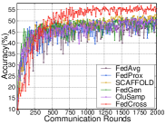
(a) CNN with $\alpha=0.1$

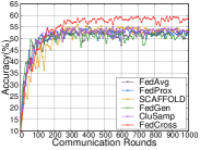
(b) CNN with $\alpha=0.5$

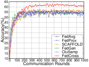
(c) CNN with $\alpha=1.0$

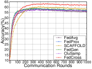
(d) CNN with IID

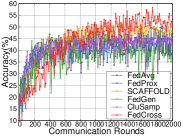
(e) ResNet-20 with $\alpha=0.1$

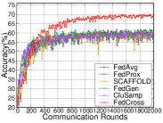
(f) ResNet-20 with $\alpha=0.5$

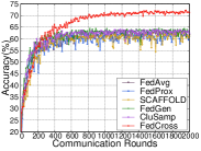
(g) ResNet-20 with $\alpha=1.0$

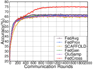
(h) ResNet-20 with IID

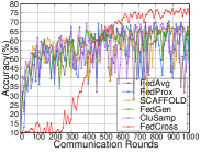
(i) VGG-16 with $\alpha=0.1$

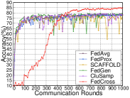
(j) VGG-16 with $\alpha=0.5$

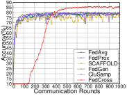
(k) VGG-16 with $\alpha=1.0$

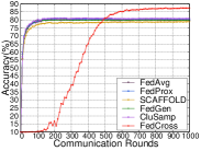
(l) VGG-16 with IID

Figure 2. Learning curves of different FL methods on CIFAR-10 dataset.

4.2.2. Comparison on the convergence speed

Figure 2 shows the convergence trends of all the FL methods (including five baselines and FedCross) on the CIFAR-10 dataset, where Figure 2(a)-2(d) are using CNN model, Figure 2(e)-2(h) are using ResNet-20 model, and Figure 2(i)-2(l) are using VGG-16 model. Note that, to evaluate the accuracy of FedCross, we conduct a global model generation process in each round and the accuracy of FedCross is calculated by the global model. From Figure 2, we can find that FedCross achieves the highest accuracy performance than the other five FL methods in both non-IID and IID scenarios. This is mainly because FedCross uses a multi-to-multi framework, which includes a fine-grained multi-model cross-aggregation mechanism. In model aggregation, the multi-model cross-aggregation method alleviates the gradient divergence, which allows multiple models to search for an optimized model in a more gentle way and avoid the stuck-at-local-search situation of the traditional coarse-grained aggregation.

From Figure 2, we can observe that the convergence of FedCross is similar to other methods when using CNN and ResNet-20 models. However, the convergence of FedCross is slower than other methods with the VGG-16 model. This is because VGG-16 is a connection-intensive model with more than 130 million parameters, while ResNet-20 only has about 30 million parameters. Thus FedCross is somewhat slower in the convergence phase.

4.2.3. Comparison on communication overhead

For FedAvg, in each training round, the communication overhead consists of $K$ models dispatching and $K$ models upload, where $K$ is the number of clients. Although FedCross uses multiple models for FL training, it does not increase any communication overhead than FedAvg. In FedCross, each client that participates in training receives only one model and uploads one trained model. Therefore the communication overhead of FedCross is only $2K$ models, which is the same as FedAvg. For FedProx and CluSamp, since their communication does not involve parameters other than models, their communication overhead is also the same as FedAvg. For SCAFFOLD, its communication overhead is $2K$ models plus $2K$ global control variables in each FL training round. Because in SCAFFOLD, the cloud server dispatches a global control variable to $K$ clients and each client uploads global control variables to the cloud server in each FL training. For FedGen, since the cloud server dispatches an additional built-in generator to $K$ clients in each FL training round, the communication overhead of FedGen is $2K$ models plus $K$ generators.

The above analysis shows that FedCross is one of the FL methods with the least communication overhead in each FL training round. As shown in Figure 2, although FedCross needs more communication rounds to achieve its best accuracy, in most cases, FedCross outperforms other methods on the accuracy comparison.

4.3. Scalability

4.3.1. Impacts of data heterogeneity

From Table 1 and Figure 2, we can observe that although FedCross alleviates the performance degradation caused by data heterogeneity, the non-IID scenarios still lead to the degradation of model performance. Furthermore, we find that in non-IID scenarios, FedCross requires more FL training rounds to converge. From Figure 2, we can find that the above situation also exists in other baselines. FedCross does better than them in the same case. Therefore, FedCross can effectively deal with various heterogeneous data scenarios.

4.3.2. Impacts of datasets

From Table 1 and Figure 2, we can observe that on the three datasets, FedCross has significantly improved FL performance, especially for datasets with complex tasks.

4.3.3. Impacts of models

From Figure 2, we can observe that for all models, FedCross can achieve significant performance improvement. Although the convergence of FedCross will be significantly slower than baselines if the model has too many parameters, FedCross is able to reach its peak before other baselines reach their peaks in the non-IID scenarios. In addition, we propose two training acceleration methods to deal with the slow convergence problem. Please see Sec. 4.4.3 for the evaluation of them.

Table 2. Test accuracy comparison with different $\alpha$ settings for three model selection criteria using CNN models on CIFAR-10 datasets in $\beta=1.0$ non-IID scenario

$\alpha$	Selection criteria
	In Order	Highest similarity	Lowest similarity
$0.5$	$56.42\pm 0.54$	$56.33\pm 0.23$	${\bf 56.81\pm 0.91}$
$0.8$	$56.66\pm 0.46$	$55.83\pm 0.85$	${\bf 57.78\pm 0.65}$
$0.9$	${\bf 58.69\pm 0.46}$	$46.91\pm 0.97$	$58.61\pm 0.48$
$0.95$	$59.12\pm 0.62$	$49.94\pm 0.94$	${\bf 59.47\pm 0.38}$
$0.99$	$59.86\pm 0.40$	$49.70\pm 1.33$	${\bf 62.16\pm 0.42}$
$0.999$	$40.85\pm 1.82$	$32.51\pm 3.39$	${\bf 46.83\pm 1.14}$

4.4. Ablation Studies

4.4.1. Evaluation of model selection strategy

Table 2 presents the performance of three model selection strategies on CIFAR-10 dataset in $\beta=1.0$ non-IID scenario. From Table 2, we can observe that Lowest Similarity can achieve the best performance with almost all the settings of $\alpha$ and the accuracy of Lowest Similarity is slightly less than In Order when $\alpha=0.9$. The Highest Similarity achieve the worst performance in all the settings of $\alpha$. This is because the Highest Similarity strategy causes the middleware models with high similarity to gradually get closer, while the models with low similarity will become far away from each, which leads to the higher aggregation difficulty of the global model. On the contrary, Lowest Similarity reduces the distance between models with low similarity at each round of aggregation, which forces all the models roughly optimize to similar directions. Referring to In Order strategy, since every two models will be aggregated after finite rounds, the similarity between models will also be limited to a certain range, but compared with Highest Similarity, its efficiency will be relatively lower. In summary, we recommend using Highest Similarity or In Order as the strategy for the selection of the collaboration model.

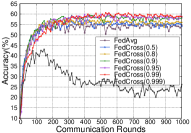
(a) In Order

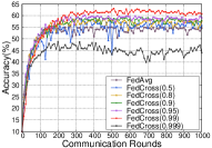
(b) Lowest Similarity

Figure 3. Learning curves of different setting of $\alpha$ using CNN models on CIFAR-10 datasets in $\beta=1.0$ non-IID scenario.

4.4.2. Evaluation of aggregation rate $\alpha$

Figure 3 presents learning curves of In Order and Lowest Similarity strategy with multiple settings of $\alpha$. In Figure 3, FedCross achieves the best performance when $\alpha=0.99$. We can also observe that as the value of $\alpha$ decreases, the performance of FedCross gradually decreases. However when $\alpha=0.999$, the performance of FedCross will drop sharply. This is because the value of $\alpha$ is too large, which leads to less knowledge acquisition from the collaboration model. In other words, the reduction of the distance between models in each round of aggregation can not offset the increase of model distance in each round of training. Therefore, the distance between models will gradually increase, resulting in a sharp decline in the performance of the global model. We can find that a large $\alpha$ will improve the performance of FedCross for it can make the model aggregation more fine-grained, but a too large $\alpha$ causes the sharp performance drop of the global model. In our experiments, FedCross achieves the best performance when $\alpha=0.99$. We recommend $\alpha$ to be less than 0.99.

4.4.3. Evaluation of acceleration methods

We evaluate the performance of two training acceleration methods on CIFAR-10 datasets using VGG-16 model. There are three variants of FedCross. The first variant “FedCross w/ PM” uses propeller models to speed up training in the first 100 FL rounds. The second variant “FedCross w/ DA” uses dynamic $\alpha$ to speed up training for the first 100 FL rounds. The third variant “FedCross w/ PM-DA” uses propeller models for the first 50 rounds and dynamic $\alpha$ for 51-100 rounds to speed up training. Figure 4 presents the learning curves of FedCross in non-IID ($\beta=0.1$) and IID scenarios. From Figure 4, we can find that all the variants can significantly accelerate the training, but will slightly reduce the accuracy of the model. In the non-IID scenario, the performance of the three variants is very close. In the IID scenario, the performance of “FedCross w/ PM-DA” is higher than the other two variants. For scenarios that need to deploy models in real-time, we recommend using the acceleration method to achieve a good performance in a short time at the price of a little performance loss. Please note even with the accelerated method, FedCross still outperforms all baselines.

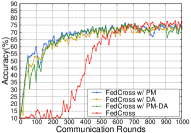
(a) non-IID Scenario with $\beta=0.1$

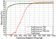
(b) IID Scenario

Figure 4. Learning curves of different training acceleration methods using VGG-16 models on CIFAR-10 datasets.

4.5. Discussion

4.5.1. Privacy preserving

Same as the traditional one-to-multi FL methods, FedCross does not need any data distribution information of each local client. For each upload model, FedCross also does not attempt to restore the user data by analyzing the model. For each dispatched model, since it is aggregated with a collaborative model, and the model is dispatched randomly, clients can not restore the user data through the model and do not know the source of received models. In addition, since the model dispatching, local training, and model update processes of FedCross are the same as FedAvg, FedCross can easily integrate many privacy-preserving techniques (Triastcyn and Faltings, 2019; Wei et al., 2020; Sun et al., 2021) used in FedAvg to reduce the privacy risks.

4.5.2. Limitations

Although FedCross has achieved extremely better performance, its low convergence speed on complex models is an important limitation. Although our proposed acceleration method can alleviate this problem, it also leads to a slight decrease in performance. Therefore, we need a more powerful acceleration method that does not damage the performance. Furthermore, at present, we only consider the scenario of heterogeneous data, and FedCross cannot adapt to the scenario of the heterogeneous model. These will be researched in our future work.

5. Conclusion

Along with the increasing prosperity of Artificial Intelligence (AI) and Internet of Things (IoT) techniques, Federated Learning (FL) has been widely acknowledged as a promising way to enable the knowledge sharing among different clients without compromising their data privacy. Although various methods have been proposed to optimize the FL classification performance, most of them are based on the traditional local model aggregation scheme, where the cloud only keeps one global model. Due to the inconsistent convergence directions of local models, such a multiple-to-one training scheme can easily result in slow convergence as well as low classification accuracy, especially for non-IID scenarios. To address this problem, this paper presents a novel FL framework named FedCross, which adopts a novel multiple-to-multiple training scheme. During the FL training, FedCross maintains a small set of intermediate models on the cloud for the purpose of weighted fusion of similar local models. Since Fedcross sufficiently respects the convergence characteristics of individual clients without averaging their local models in a rude manner, the local models can quickly converge to their local optimum counterparts for classification. Comprehensive experimental results on well-known datasets show that FedCross outperforms state-of-the-art FL methods significantly in both IID and non-IID scenarios without resulting in extra communication overhead.

(a) CNN with $\alpha=0.1$

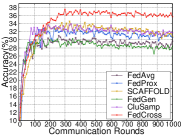
(b) CNN with $\alpha=0.5$

(c) CNN with $\alpha=1.0$

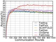
(d) CNN with IID

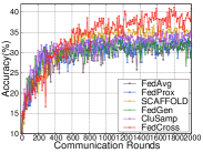
(e) ResNet-20 with $\alpha=0.1$

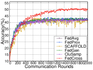
(f) ResNet-20 with $\alpha=0.5$

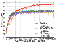
(g) ResNet-20 with $\alpha=1.0$

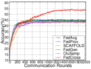
(h) ResNet-20 with IID

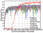
(i) VGG-16 with $\alpha=0.1$

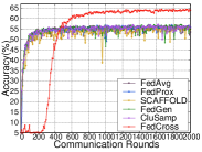
(j) VGG-16 with $\alpha=0.5$

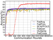
(k) VGG-16 with $\alpha=1.0$

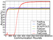
(l) VGG-16 with IID

Figure 5. Learning curves of different FL methods on CIFAR-100 dataset.

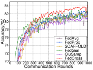
(a) CNN

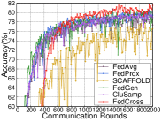
(b) ResNet-20

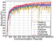
(c) VGG-16

Figure 6. Learning curves of different FL methods on FEMNIST dataset.

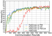
(a) non-IID $\beta=0.1$

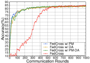
(b) non-IID $\beta=0.5$

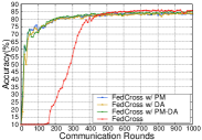
(c) non-IID $\beta=1.0$

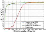
(d) IID

Figure 7. Learning curves of different training acceleration methods using VGG-16 models on CIFAR-10 datasets.

6. Appendix

6.1. Experimental Results for Accuracy Comparison

In this section we presents all the experimental results. Figure 5 compare the learning curves of FedCross with all the five baselines on CIFAR-100 datasets. Figure 6 compare the learning curves of FedCross with all the five baselines on FEMNIST datasets. Figure 7 presents learning curves of different training acceleration methods using VGG-16 models on CIFAR-10 datasets.

References

- (1)
- Caldas et al. (2018) Sebastian Caldas, Sai Meher Karthik Duddu, Peter Wu, Tian Li, Jakub Konečnỳ, H Brendan McMahan, Virginia Smith, and Ameet Talwalkar. 2018. Leaf: A benchmark for federated settings. arXiv preprint arXiv:1812.01097 (2018).
- Chen et al. (2020) Cheng Chen, Ziyi Chen, Yi Zhou, and Bhavya Kailkhura. 2020. Fedcluster: Boosting the convergence of federated learning via cluster-cycling. In Proceedings of International Conference on Big Data (Big Data). 5017–5026.
- Cui et al. (2021) Yangguang Cui, Kun Cao, Guitao Cao, Meikang Qiu, and Tongquan Wei. 2021. Client scheduling and resource management for efficient training in heterogeneous IoT-edge federated learning. IEEE Transactions on Computer-Aided Design of Integrated Circuits and Systems (2021).
- Fraboni et al. (2021) Yann Fraboni, Richard Vidal, Laetitia Kameni, and Marco Lorenzi. 2021. Clustered sampling: Low-variance and improved representativity for clients selection in federated learning. In Proceedings of International Conference on Machine Learning (ICML). 3407–3416.
- He et al. (2016) Kaiming He, Xiangyu Zhang, Shaoqing Ren, and Jian Sun. 2016. Deep residual learning for image recognition. In Proceedings of the conference on computer vision and pattern recognition (CVPR). 770–778.
- Hsu et al. (2019) Tzu-Ming Harry Hsu, Hang Qi, and Matthew Brown. 2019. Measuring the effects of non-identical data distribution for federated visual classification. arXiv preprint arXiv:1909.06335 (2019).
- Huang et al. (2021) Yutao Huang, Lingyang Chu, Zirui Zhou, Lanjun Wang, Jiangchuan Liu, Jian Pei, and Yong Zhang. 2021. Personalized Cross-Silo Federated Learning on Non-IID Data.. In Proceedings of the AAAI Conference on Artificial Intelligence (AAAI). 7865–7873.
- Kairouz et al. (2021) Peter Kairouz, H Brendan McMahan, Brendan Avent, Aurélien Bellet, Mehdi Bennis, Arjun Nitin Bhagoji, Kallista Bonawitz, Zachary Charles, Graham Cormode, Rachel Cummings, et al. 2021. Advances and open problems in federated learning. Foundations and Trends® in Machine Learning 14, 1–2 (2021), 1–210.
- Karimireddy et al. (2020) Sai Praneeth Karimireddy, Satyen Kale, Mehryar Mohri, Sashank Reddi, Sebastian Stich, and Ananda Theertha Suresh. 2020. Scaffold: Stochastic controlled averaging for federated learning. In Proceedings of International Conference on Machine Learning (ICML). 5132–5143.
- Krizhevsky et al. (2009) Alex Krizhevsky, Geoffrey Hinton, et al. 2009. Learning multiple layers of features from tiny images. (2009).
- Li et al. (2021a) Ang Li, Jingwei Sun, Pengcheng Li, Yu Pu, Hai Li, and Yiran Chen. 2021a. Hermes: an efficient federated learning framework for heterogeneous mobile clients. In Proceedings of International Conference on Mobile Computing and Networking (MobiCom). 420–437.
- Li et al. (2021b) Anran Li, Lan Zhang, Junhao Wang, Juntao Tan, Feng Han, Yaxuan Qin, Nikolaos M Freris, and Xiang-Yang Li. 2021b. Efficient federated-learning model debugging. In Proceedings o International Conference on Data Engineering (ICDE). 372–383.
- Li et al. (2022) Qinbin Li, Yiqun Diao, Quan Chen, and Bingsheng He. 2022. Federated learning on non-iid data silos: An experimental study. In Proceedings of International Conference on Data Engineering (ICDE). 965–978.
- Li et al. (2020) Tian Li, Anit Kumar Sahu, Manzil Zaheer, Maziar Sanjabi, Ameet Talwalkar, and Virginia Smith. 2020. Federated optimization in heterogeneous networks. Proceedings of Machine Learning and Systems 2 (2020), 429–450.
- Li and Zhan (2021) Xin-Chun Li and De-Chuan Zhan. 2021. Fedrs: Federated learning with restricted softmax for label distribution non-iid data. In Proceedings of ACM SIGKDD Conference on Knowledge Discovery & Data Mining (KDD). 995–1005.
- Lim et al. (2021) Wei Yang Bryan Lim, Jer Shyuan Ng, Zehui Xiong, Jiangming Jin, Yang Zhang, Dusit Niyato, Cyril Leung, and Chunyan Miao. 2021. Decentralized edge intelligence: A dynamic resource allocation framework for hierarchical federated learning. IEEE Transactions on Parallel and Distributed Systems (TPDS) 33, 3 (2021), 536–550.
- Lin et al. (2020) Tao Lin, Lingjing Kong, Sebastian U Stich, and Martin Jaggi. 2020. Ensemble distillation for robust model fusion in federated learning. Advances in Neural Information Processing Systems 33 (2020), 2351–2363.
- Liu et al. (2022) Jianchun Liu, Yang Xu, Hongli Xu, Yunming Liao, Zhiyuan Wang, and He Huang. 2022. Enhancing Federated Learning with Intelligent Model Migration in Heterogeneous Edge Computing. In Proceedings of International Conference on Data Engineering (ICDE). 1586–1597.
- Luo et al. (2021b) Bing Luo, Xiang Li, Shiqiang Wang, Jianwei Huang, and Leandros Tassiulas. 2021b. Cost-effective federated learning in mobile edge networks. IEEE Journal on Selected Areas in Communications 39, 12 (2021), 3606–3621.
- Luo et al. (2021a) Mi Luo, Fei Chen, Dapeng Hu, Yifan Zhang, Jian Liang, and Jiashi Feng. 2021a. No fear of heterogeneity: Classifier calibration for federated learning with non-iid data. Advances in Neural Information Processing Systems 34 (2021), 5972–5984.
- McMahan et al. (2017) Brendan McMahan, Eider Moore, Daniel Ramage, Seth Hampson, and Blaise Aguera y Arcas. 2017. Communication-efficient learning of deep networks from decentralized data. In Proceedings of Artificial intelligence and statistics. 1273–1282.
- Ozkara et al. (2021) Kaan Ozkara, Navjot Singh, Deepesh Data, and Suhas Diggavi. 2021. QuPeD: Quantized Personalization via Distillation with Applications to Federated Learning. Advances in Neural Information Processing Systems 34 (2021), 3622–3634.
- Pytorch (2022) Pytorch. 2022. Models and pre-trained weight. https://pytorch.org/vision/stable/models.html.
- Rey et al. (2022) Valerian Rey, Pedro Miguel Sánchez Sánchez, Alberto Huertas Celdrán, and Gérôme Bovet. 2022. Federated learning for malware detection in iot devices. Computer Networks 204 (2022), 108693.
- Sattler et al. (2021) Felix Sattler, Tim Korjakow, Roman Rischke, and Wojciech Samek. 2021. Fedaux: Leveraging unlabeled auxiliary data in federated learning. IEEE Transactions on Neural Networks and Learning Systems (2021).
- Simonyan and Zisserman (2014) Karen Simonyan and Andrew Zisserman. 2014. Very deep convolutional networks for large-scale image recognition. arXiv preprint arXiv:1409.1556 (2014).
- Sun et al. (2021) Lichao Sun, Jianwei Qian, and Xun Chen. 2021. LDP-FL: Practical Private Aggregation in Federated Learning with Local Differential Privacy. In Proceedings of International Joint Conference on Artificial Intelligence (IJCAI). 1571–1578.
- Triastcyn and Faltings (2019) Aleksei Triastcyn and Boi Faltings. 2019. Federated learning with bayesian differential privacy. In Proceedings of International Conference on Big Data (Big Data). 2587–2596.
- Uddin et al. (2020) Md Palash Uddin, Yong Xiang, Xuequan Lu, John Yearwood, and Longxiang Gao. 2020. Mutual information driven federated learning. IEEE Transactions on Parallel and Distributed Systems (TPDS) 32, 7 (2020), 1526–1538.
- Wang et al. (2020) Hao Wang, Zakhary Kaplan, Di Niu, and Baochun Li. 2020. Optimizing federated learning on non-iid data with reinforcement learning. In Proceedings of Conference on Computer Communications (INFOCOM). 1698–1707.
- Wei et al. (2020) Kang Wei, Jun Li, Ming Ding, Chuan Ma, Howard H Yang, Farhad Farokhi, Shi Jin, Tony QS Quek, and H Vincent Poor. 2020. Federated learning with differential privacy: Algorithms and performance analysis. IEEE Transactions on Information Forensics and Security 15 (2020), 3454–3469.
- Wu et al. (2021) Jinze Wu, Qi Liu, Zhenya Huang, Yuting Ning, Hao Wang, Enhong Chen, Jinfeng Yi, and Bowen Zhou. 2021. Hierarchical personalized federated learning for user modeling. In Proceedings of the Web Conference (WWW). 957–968.
- Wu et al. (2020) Wentai Wu, Ligang He, Weiwei Lin, and Rui Mao. 2020. Accelerating federated learning over reliability-agnostic clients in mobile edge computing systems. IEEE Transactions on Parallel and Distributed Systems (TPDS) 32, 7 (2020), 1539–1551.
- Yang et al. (2021) Chengxu Yang, Qipeng Wang, Mengwei Xu, Zhenpeng Chen, Kaigui Bian, Yunxin Liu, and Xuanzhe Liu. 2021. Characterizing impacts of heterogeneity in federated learning upon large-scale smartphone data. In Proceedings of the Web Conference (WWW). 935–946.
- Yang et al. (2019) Qiang Yang, Yang Liu, Tianjian Chen, and Yongxin Tong. 2019. Federated machine learning: Concept and applications. ACM Transactions on Intelligent Systems and Technology (TIST) 10, 2 (2019), 1–19.
- Zhang et al. (2021) Jingwen Zhang, Yuezhou Wu, and Rong Pan. 2021. Incentive mechanism for horizontal federated learning based on reputation and reverse auction. In Proceedings of the Web Conference (WWW). 947–956.
- Zhang et al. (2022) Lin Zhang, Li Shen, Liang Ding, Dacheng Tao, and Ling-Yu Duan. 2022. Fine-tuning global model via data-free knowledge distillation for non-iid federated learning. In Proceedings of the IEEE/CVF Conference on Computer Vision and Pattern Recognition (CVPR). 10174–10183.
- Zhang et al. (2020) Xinqian Zhang, Ming Hu, Jun Xia, Tongquan Wei, Mingsong Chen, and Shiyan Hu. 2020. Efficient federated learning for cloud-based AIoT applications. IEEE Transactions on Computer-Aided Design of Integrated Circuits and Systems (TCAD) 40, 11 (2020), 2211–2223.
- Zhu et al. (2021) Zhuangdi Zhu, Junyuan Hong, and Jiayu Zhou. 2021. Data-free knowledge distillation for heterogeneous federated learning. In Proceedings of International Conference on Machine Learning (ICML). 12878–12889.
- Zhuang et al. (2020) Weiming Zhuang, Yonggang Wen, Xuesen Zhang, Xin Gan, Daiying Yin, Dongzhan Zhou, Shuai Zhang, and Shuai Yi. 2020. Performance optimization of federated person re-identification via benchmark analysis. In Proceedings of ACM International Conference on Multimedia (MM). 955–963.