Reinforcement Learning for ConnectX

Abstract

ConnectX is a two-player game that generalizes the popular game Connect 4. The objective is to get X coins across a row, column, or diagonal of an M x N board. The first player to do so wins the game. The parameters (M, N, X) are allowed to change in each game, making ConnectX a novel and challenging problem. In this paper, we present our work on the implementation and modification of various reinforcement learning algorithms to play ConnectX.

1 Introduction

Connect 4 is a popular board game in which two players alternately take turns dropping their respective tokens on a $6\times 7$ board by choosing the column they wish to drop their token in. The token falls down to the lowest unoccupied cell in the column, and if all six cells in a column are occupied, the move is declared illegal. The players’ objective is to place tokens so that there are 4 of their tokens consecutively across either a row or a column or a diagonal, and the first player to do so wins the game. Connect 4 has been solved [2], and it has been proved that the player who starts the game has a guaranteed-to-win strategy.

ConnectX is a generalization of Connect 4 that allows for variable board sizes and number of tokens to be connected (referred to as ’inarow’ hereafter). Hence, each time a player plays ConnectX, the board size and inarow may differ. This generalization makes the problem of optimally playing the game significantly more difficult. Guaranteed-to-win-or-draw strategies might exist for small board sizes and inarow lesser than 4, but no such strategy is known beyond these constraints. Therefore, a general method to play ConnectX is needed, and Reinforcement Learning is well-suited for the problem.

The following algorithms are implemented and modified to play ConnectX:

• Greedy or One-Step Lookahead

• Monte Carlo Tree Search (MCTS)

• Minimax with alpha-beta pruning

• MCTS-minimax hybrid

• AlphaZero

MCTS-minimax hybrid is a novel algorithm which modifies MCTS to use informed rollouts, relying on minimax search, instead of random ones.

All these algorithms were implemented on an open-source ConnectX environment provided by Kaggle. The algorithms were played against one another and also submitted to a ConnectX competition hosted by Kaggle, where all submissions to the competition are matched by their position on the leaderboard, similar submissions played against each other, and the game’s result used to update the leaderboard.

We were able to successfully implement the above mentioned algorithms, and their performances have been evaluated in section 5. AlphaZero was the best performing algorithm, and we were able to achieve a leaderboard position of 9 (out 225 participating teams) with it.

2 Related work

To the best of our knowledge, there exists no previous work directly associated to playing ConnectX using Reinforcement Learning. On the other hand, Connect 4 has seen a lot of work, and serves as a good game to test algorithms. Connect 4 was first solved by James Dow Allen (October 1, 1988), and independently by Victor Allis (October 16, 1988) [2]. Reference [1] explores Connect 4 in great detail, and provides optimal strategies for both the players. Connect 4 has also been solved in a brute-force manner by the following apporaches:

• An 8-ply database [14]

• NegaMax / MiniMax using alpha-beta pruning

• NegaMax / MiniMax using transposition tables

Monte Carlo Tree Search [5] (MCTS) is a popular framework that is well-applicable to problems where the environment can be simulated, but heuristics about good actions are unavailable. MCTS was combined with neural networks and the resulting algorithm AlphaGo [12] performed extremely well in the board game of Go. This algorithm was then extended to other games whereby domain specific knowledge was removed from the algorithm to make it more general and thereby came the algorithm of AlphaZero, which we have adapted to ConnectX. The AlphaZero algorithm as described in [11] has been used to play various games like chess, go and shogi. However, extensions to similarly characterized games like Othello, Connect 4, and GoBang have also been made.

Some variants of MCTS [4] [3] incorporate minimax updates or heuristics to improve MCTS’s performance. Variants that propagate proven wins/losses have been designed too and tested to be empirically better in games of sudden death [15]. MCTS has been adapted to play a plethora of games as in [9] [7] [6] [10] [8], and has seen tremendous success.

3 Defining the problem

An instance of the game is parameterized by $(M,N,X)$, where $M$ is the number of rows in the board, $N$ the columns, and $X$ is the inarow parameter. A $player$ is given the current state of the board ($board$) and indication of the token he has to play ($mark$), and it must return a value $a\in\{0,...,N-1\}$ denoting the column it wants to place the token $mark$ in. If the game ends (due to a win/draw/illegal move for $mark$), the simulation is stopped. If not, the opponent is provided the new $board$ and $mark$ for choosing a move. In the Kaggle environment, each $player$ has 5 seconds to choose their move, and if the $player$ fails to do so, it is automatically declared as the loser. An illegal choice of move also results in an immediate loss.

We hence want to design a function $player:board\times mark\rightarrow\{0,1,...,N-1\}$ that attempts to be the first player to get $X$ in a row on a board of size $M\times N$.

4 Methodology

4.1 The greedy algorithm

Algorithm 1 was implemented to act as a baseline, and to get a better idea of the functioning of the Kaggle environment and submissions.

Algorithm 1 Greedy Algorithm

$board,mark$

$value_{i}\leftarrow 0\ \forall i\in\{0,1,...,N-1\}$

for $i\in\{0,1,...,N-1\}$ do

     if placing $mark$ in column $i$ connects $X$ in a row for $mark$ then

         $value_{i}\leftarrow\infty$

     end if

     return $a=arg\max_{i}value_{i}$

end for

4.2 Plain Monte Carlo Tree Search

Each round of MCTS uses the following steps in order:

• Selection: Starting from the current state, the move (and hence the next state) is chosen via a Upper-Confidence-Bound-like method that represents values of sub-trees. The exact formulation is:

  $$UCB(\text{Tree rooted at state }S) =\frac{w_{S}}{n_{S}}+c\cdot\sqrt{\frac{ln\ N_{S}}{n_{S}}}$$

  $$where:$$

  $$w_{S} =\text{The number of winning simulations from state }S$$

  $$n_{S} =\text{The total number of simulations from state }S$$

  $$N_{s} =\text{The total number of simulations from the parent of state }S$$

  $$c =\sqrt{2}\ (\text{in our implementation})$$

  At each selection step, MCTS chooses the child state with the highest UCB(tree) value. This selection is repeated until a state that has atleast one unsimulated child is reached.

• Expansion: If the state at the end of selection is a terminal state, we skip to the backpropagation step. Otherwise, we pick a random valid move, and initialize a tree node representing the new state seen.

• Simulation: The new state seen is simulated. In plain MCTS, random legal moves are played till the game ends, and the result of this random playout is then backpropagated.

• Backpropagation: The path from the expanded state to the root state is traced, and the $w$ and $n$ for each of these states is updated based on whether the simulation was a win or a loss. A draw is treated as half a win.

4.3 Minimax

Algorithm 2 is a standard alpha-beta pruned minimax algorithm that was implemented. A search depth of 5 was chosen in accordance with 5 second move timeout. The heuristic used was as follows:

$$heuristic= \sum_{i=2}^{X}1000^{i-1}\cdot\texttt{\# occurrences of i mark-tokens in a row}\ -$$

$$\sum_{i=2}^{X}2000^{i-1}\cdot\texttt{\# occurrences of i opponent-mark-tokens in a row}$$

Here, 1000 and 2000 are empirically chosen constants.

Algorithm 2 Alpha-Beta pruned minimax algorithm

$board,mark,heuristic$

function minimax(state, depth, $\alpha$, $\beta$, maximizingPlayer)

     if depth = 0 or game ended then

         return $heuristic(state,mark)$

     end if

     if maximizingPlayer then

         $value\leftarrow-\infty$

         for each legal move do

              state’ $\leftarrow$ state reached by playing this move

              $value\leftarrow max(value,MINIMAX(state^{\prime},depth-1,\alpha,\beta,FALSE)$

              if $value\geq\beta$ then

                  break

              end if

              $\alpha=max(\alpha,value)$

         end for

     else

         $value\leftarrow\infty$

         for each legal move do

              state’ $\leftarrow$ state reached by playing this move

              $value\leftarrow min(value,MINIMAX(state^{\prime},depth-1,\alpha,\beta,TRUE)$

              if $value\leq\alpha$ then

                  break

              end if

              $\beta=min(\beta,value)$

         end for

     end if

end function

MINIMAX(board, 5, $-\infty$, $\infty$, TRUE)

4.4 MCTS with minimax rollouts

We implemented a variation of plain MCTS by changing the Simulation step. Shallow minimax searches were used to guide the rollouts instead of random moves. A search depth of 2 was used, and all other steps were identical to that of plain MCTS. Since minimax rollouts slowed down each simulation by a significant amount, the number of iterations the algorithm could run per move dropped and hence, $c$ for the calculation of UCB was reduced to $\frac{1}{\sqrt{2}}$. A smaller $c$ was seen to empirically improve performance, and it can be argued having a smaller horizon calls for lesser (and better) exploration (and hence a smaller $c$).

4.5 AlphaZero

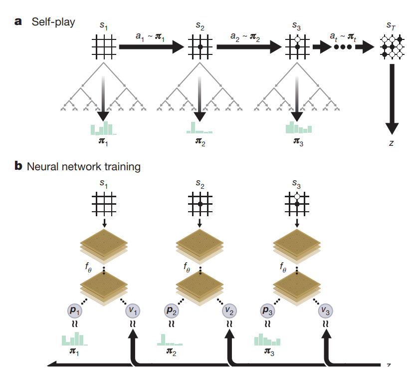
Figure 1: Self Play reinforcement learning in AlphaZero taken from [13]

The AlphaZero algorithm uses MCTS to initialize a search on the game tree and generates data on the game. This is called as the self play stage. At each step the action chosen is the one with the highest UCB value. This generates a probability vector $\pi$ over the moves. After the terminal state is reached the game is scored according to the rules and a win/loss/draw is declared. There is a concatenated neural network which maps the current state $s_{t}$ to both, the policy p and the value function $v_{t}$. The neural network parameters are then updated using backpropagation, with an Adam optimiser, to minimise the error in the value $v_{t}$ using MSE loss as well as the difference between the policy vector p and the search probabilities $\pi$ using cross entropy loss. Experience replay is also used here since it allows us to work with fewer simulations for each iteration since the training data keeps growing with iterations.

Algorithm 3 Policy Iteration through Self Play

$executeEpisode,\ trainNN,\ initNN,\ threshold$

function POLICY_ITERATION(numIters, numEpisodes)

     $\theta\leftarrow initNN()$

     $trainExamples\leftarrow[]$

     for $i\;in\{1,...,numIters\}$ do

         for $e\;in\{1,...,numEpisodes\}$ do

              $ex\leftarrow executeEpisode(nn)$

              $trainExamples.append(ex)$

         end for

         $\theta_{new}\leftarrow trainNN(trainExampples)$

         if percentage($\theta_{new}$ beats $\theta$) $\geq threshold$ then

              $\theta\leftarrow\theta_{new}$

         end if

     end for

end function

Algorithm 4 Execute Episode

$assignReward,MCTS,gameNextState,gameStartState$

function executeEpisode(numSims)

     $examples\leftarrow[]$

     $s\leftarrow gameStartState()$

     while True do

         for $i\;in[1,...,numSims]$ do

              $MCTS(s,\theta)$

         end for

         $examples.add((s,\pi_{s},\_))$

         $a*\sim\pi_{s}$

         $s\leftarrow gameNextState(s,a*)$

         if $gameEnded(s)$ then

              $//{Fill\;\_\;with\;rewards\;in\;examples,\;the\;backpropagation\;step\;for\;MCTS}$

              $examples\leftarrow assignReward(examples)$

              break and return $examples$

         end if

     end while

end function

After training, the new network is played against the older network before the current round of training. And if the new network performs sufficiently better compared to the previous one,i.e., out of the total decided games which were played (not draw) if the fraction is decided games won by newer network is above a certain threshold (0.6 in our case), the network in use is updated and otherwise the newer network is not used.

Since ConnectX does not fix the size of the board beings used it poses a problem since the input state size is not always fixed. The workaround we found for that is using padding to make the input size always as $12\times 12$ so that the state is always fully represented. The number was chosen at random based on how the board sizes varied during the competition.

5 Results

Table 1: Comparison of agents

Algorithms	Greedy	Plain MCTS	Minimax	MCTS-minimax hybrid	AlphaZero
Greedy	-	10 / 0 / 0	10 / 0 / 0	10 / 0 / 0	10 / 0 / 0
Plain MCTS	-	-	2 / 8 / 0	2 / 8 / 0	7 / 1/ 2
Minimax	-	-	-	6 / 2 / 2	10 / 0 / 0
MCTS-minimax hybrid	-	-	-	-	9 / 0 / 1

Table 1 compares the performance of the various agents implemented. Each agent plays a total of 10 games against every other agent, and the score is calculated as follows:
For comparing algorithm $i$ in row $i$ against algorithm $j$ in column $j$, the first number is the number of times $j$ wins, the second is the number of times $i$ wins (or $j$ looses) and the third number is the number of draws.

Table 2: Kaggle score of agents

Algorithms	Score
Greedy	268
Plain MCTS	1075
Minimax	873
MCTS-minimax hybrid	980
AlphaZero	1282

Table 2 lists the scores of our submissions of the implemented algorithms on Kaggle competition for ConnectX. The scoring system in Kaggle works as follows: each submission is initialised with a fixed score of 600, then the submissions are played against one another and the score of the winning submission increases while that of the losing submission decreases (proportional to the difference in their ’skill’). In case of a draw the score of the submission with the lower score increases while the submission with the higher score loses some points.

The final scores of all our submissions have been recorded in table 2. All the submissions except the greedy algorithm have scored over 600, at which they were initialized. These scores are also consistent with the performance we get when we play the agents against one another. The competition also maintains a leaderboard which ranks a user according to their best submission. AlphaZero, which is our best agent, has landed us at the 9th position on the leaderboard out of 225 teams with around 700 submissions as on May 5, 2022. This is much better than our initial goal of being in the Top-25, and our revised goal after the mid-stage presentation of being in the Top-15.

As is evident from table 1 and table 2, the plain MCTS agent did better than the hybrid MCTS agent with minimax based rollouts. The reason for this can be attributed to the fact that the hybrid agent is able to do much fewer simulations (around 500 per move) as compared to the plain MCTS agent (20000 simulations per move) on account of the computation cost of minimax searches for every rollout. However, since each simulation for the hybrid agent is much more efficient than that of the plain MCTS agent, the hybrid agent does not perform significantly worse (inspite of the severe shortage of iterations that MCTS requires to converge).

The results that we have obtained as a part of this project show how various algorithms play out when deployed in a simple-ruled yet difficult-to-learn game. Using our findings, we can claim that certain algorithms are better than others under the given conditions. Games are used to test algorithms since they are able to mimic specific real world game-theory problems in a compact and specific way. Hence, these results also work as a proof of concept for the algorithms.

6 Conclusion and Future Outlook

From our results, we see how various algorithms perform when they are played against one another. This helped us to rank these algorithms. The Kaggle submission further provided us with validation for our results and provided us with a baseline to compare the different agents. Hence, as concluded in [11] as well, we can say that AlphaZero is the best amongst the other algorithms tried for playing ConnectX.

One possible direction of future work is improvement in the AlphaZero algorithm. We have only used a basic architecture for the neural network, and the hyperparameters haven’t been finely tuned. With the availability of sufficient time and compute power, this can be done to further improve the performance of AlphaZero. Since we are still only at the 9th position on the leaderboard of the competition, there is room for improvement to be made.

We note that all of our algorithms had very little, if at all any, dependency on domain knowledge of ConnectX (the obvious exception being the heuristic used in minimax). We believe that such general algorithms are the way to go, and the success self-play based AlphaZero further strengthens our belief. This, however, requires large amount of computational resources for game simulation and larger neural networks along with set baselines with which to compare, like Stockfish for chess and Elmo for shogi, or a competition like the one we have used for ConnectX, which are not easily available for other games.

References

- [1] James Dow Allen “The Complete Book of Connect 4: History, strategy, puzzles” Sterling, 2010
- [2] Victor Allis “A knowledge-based approach to connect-four. The game is solved: White wins” In Master’s thesis, Vrije Universiteit, 1988, pp. 4
- [3] Hendrik Baier and Mark Winands “Monte-Carlo Tree Search and minimax hybrids” In IEEE Conference on Computatonal Intelligence and Games, CIG, 2013, pp. 1–8 DOI: 10.1109/CIG.2013.6633630
- [4] Hendrik Baier and Mark Winands “Monte-Carlo Tree Search and Minimax Hybrids with Heuristic Evaluation Functions”, 2014, pp. 45–63 DOI: 10.1007/978-3-319-14923-3_4
- [5] Guillaume Chaslot, Sander Bakkes, Istvan Szita and Pieter Spronck “Monte-Carlo Tree Search: A New Framework for Game AI.” In Bijdragen, 2008
- [6] Levente Kocsis, Csaba Szepesvári and Jan Willemson “Improved Monte-Carlo Search”, 2006
- [7] “M. H. M. Winands, Y. Bjornsson, and J.-t. Saito, “Monte Carlo ¨ Tree Search in Lines of Action,” IEEE Trans. Comp. Intell. AI Games, vol. 2, no. 4, pp. 239–250, 2010.”
- [8] J.P.A.M. Nijssen and Mark Winands “Monte-Carlo Tree Search for the Game of Scotland Yard”, 2011, pp. 158–165 DOI: 10.1109/CIG.2011.6032002
- [9] Tapani Raiko and Jaakko Peltonen “Application of UCT Search to the Connection Games of Hex, Y, *Star, and Renkula!”, 2008
- [10] Jonathan Rubin and Ian Watson “Computer poker: A review” Special Review Issue In Artificial Intelligence 175.5, 2011, pp. 958–987 DOI: https://doi.org/10.1016/j.artint.2010.12.005
- [11] David Silver et al. “Mastering Chess and Shogi by Self-Play with a General Reinforcement Learning Algorithm” arXiv, 2017 DOI: 10.48550/ARXIV.1712.01815
- [12] David Silver et al. “Mastering the game of Go with deep neural networks and tree search” In Nature 529, 2016, pp. 484–489 DOI: 10.1038/nature16961
- [13] David Silver et al. “Mastering the game of Go without human knowledge” In Nature 550.7676, 2017, pp. 354–359 DOI: 10.1038/nature24270
- [14] John Tromp “Connect-4 Data Set” [UCI Machine Learning Repository], 1995
- [15] Mark Winands, Yngvi Björnsson and Jahn-Takeshi Saito “Monte-Carlo Tree Search Solver”, 2008, pp. 25–36 DOI: 10.1007/978-3-540-87608-3_3