A time-periodic competition model with nonlocal dispersal and bistable nonlinearity: propagation dynamics and stability

Abstract: Seasonality frequently occurs in population models, and the corresponding seasonal patterns have been of great interest to scientists. This paper is concerned with traveling waves to a time-periodic bistable Lotka-Volterra competition system with nonlocal dispersal. We first establish the existence, uniqueness and stability of traveling wave solutions for this system. Then, by utilizing comparison principle and the stability property, the relationship among the bistable wave speed, the asymptotic propagation speeds of the associated monotone subsystems and the speed of upper/lower solutions is obtained. Next, explicit sufficient conditions for positive and negative bistable wave speeds are derived. Our explicit results are derived by constructing particular upper/lower solutions with specific asymptotical behaviors, which can be seen as case studies shedding light on further studies and improvements. Finally, the theoretical results are corroborated under weak conditions by direct simulations of the underlying time-periodic system with nonlocal dispersal. The combined impact of competition, dispersal and seasonality on the invasion direction has shed new light on the modelings and analysis of population competition and species invasion in heterogeneous media.

Keywords: Bistable traveling wave, existence, stability, Lotka-Volterra competition model, nonlocal dispersal, invasion direction.

2000 Mathematics Subject Classification. Primary 35K57, 35C07,37C65, 92D25.

1 Introduction

In this paper we are concerned with traveling wave solutions to the following nonlocal dispersal system

$$\left\{\begin{array}[]{lr}u_{t}=d_{1}(t)\,[J_{1}\ast u-u]+u(r_{1}(t)-a_{1}(t)u-b_{1}(t)v),\\ v_{t}=d_{2}(t)\,[J_{2}\ast v-v]+v(r_{2}(t)-a_{2}(t)u-b_{2}(t)v),\end{array}\text{$x\in\mathbb{R},\,\,t>0,$}\right.$$ (1.1)

where $u=u(x,t)$ and $v=v(x,t)$ stand for the densities of two competitive species at position $x$ at time $t;$ the functions $d_{i}(t)$ are the dispersal coefficients, $r_{i}(t)$ are the net birth rates or resource strength, $r_{i}(t)/a_{i}(t)$ are called the carrying capacities, $b_{i}(t)/r_{i}(t)$ are the competition coefficients, $J_{i}$ represent the kernel functions,   $i=1,2.$ The convolution $J_{i}\ast\omega(x,t)$ means

$$J_{i}\ast\omega(x,t)=\int_{\mathbb{R}}J_{i}(x-y)\omega(y,t)\,dy$$

for any continuous function $\omega(x,t)$. Moveover, we assume that all the coefficients are continuous positive T-periodic functions and satisfy the bistable nonlinearity

$$\int_{0}^{T}a_{1}(t)p(t)-b_{1}(t)q(t)\ dt<0,\,\,\,\int_{0}^{T}b_{2}(t)q(t)-a_{2}(t)p(t)\ dt<0,$$ (1.2)

where

$$\left\{\begin{array}[]{lr}p(t)=\dfrac{p_{0}e^{\int_{0}^{t}r_{1}(s)ds}}{1+p_{0}\int_{0}^{t}e^{\int_{0}^{s}r_{1}(\tau)d\tau}a_{1}(s)ds},\,\,\,\,p_{0}=\dfrac{e^{\int_{0}^{T}r_{1}(s)ds}-1}{\int_{0}^{T}e^{\int_{0}^{s}r_{1}(\tau)d\tau}a_{1}(s)ds}>0,\\[5.69054pt] q(t)=\dfrac{q_{0}e^{\int_{0}^{t}r_{2}(s)ds}}{1+q_{0}\int_{0}^{t}e^{\int_{0}^{s}r_{2}(\tau)d\tau}b_{2}(s)ds},\,\,\,\,q_{0}=\dfrac{e^{\int_{0}^{T}r_{2}(s)ds}-1}{\int_{0}^{T}e^{\int_{0}^{s}r_{2}(\tau)d\tau}b_{2}(s)ds}>0.\end{array}\right.$$ (1.3)

Competition among species is an eternal topic in nature. In recent years, Lotka-Volterra type systems with nonlocal dispersal have been frequently applied to describe the dynamic interactions between two competing species, see e.g., [3, 26, 27, 6, 23, 8, 25, 17, 13]. Among them, Yu and Yuan in [25] established the existence of traveling wave solutions to a nonlocal dispersal competitive-cooperative system by using the Schauder’s fixed-point theorem and a cross-iteration technique. Li and Lin [17] proved the existence of traveling wavefronts in a nonlocal dispersal cooperative system with delays by the method of upper and lower solutions. Bao, Li and Shen [3] investigated the existence and non-existence of space-periodic traveling wave solutions of a competition system with nonlocal dispersal and space-periodic coefficients by means of the monotone semiflow theory. When all the coefficients are constant, the system in (1.1) becomes

$$\left\{\begin{array}[]{lr}u_{t}=d_{1}\,[J_{1}\ast u-u]+u(r_{1}-a_{1}u-b_{1}v),\\ v_{t}=d_{2}\,[J_{2}\ast v-v]+v(r_{2}-a_{2}u-b_{2}v),\end{array}\right.x\in\mathbb{R},\,t>0,$$ (1.4)

which has been studied in [26, 8, 22]. Zhang, Ma and Li in [26] showed that the bistable traveling waves with nonzero speed are strictly monotone. Pan and Lin [22] proved the existence of the traveling waves of system (1.4) with speed $c>c^{*}$ for a critical speed $c^{*}$, by constructing upper and lower solutions and using a limiting process. Fang and Zhao [8] showed that the minimal wave speed must be the spreading speed, when monostable-nonlinearity is assumed. Dynamics for related diffusive Lotka-Velterra competitive models have been extensively studied in [1, 5, 9, 10, 28, 11, 12, 15, 16, 21].

In this paper, we further study traveling wave solutions of Lotka-Volterra competition model (1.1) when seasonality is coupled with nonlocal dispersal. Throughout this paper, we will use the notation

$$\overline{f}=\frac{1}{T}\int_{0}^{T}f(t)\,dt$$

to denote the average value of a function on the interval $[0,T]$ and always assume the following:
(A1) $J_{i}$ is nonnegative and Lebesgue measurable for each $i;$
(A2) For any $\lambda\in\mathbb{R},$ $\int_{\mathbb{R}}J_{i}(x)e^{-\lambda x}\,dx<\infty;$
(A3) $\int_{\mathbb{R}}J_{i}(x)dx=1,~{}x\in\mathbb{R}.$

Under the condition (1.2), the corresponding kinetic system of (1.1)

$$\left\{\begin{array}[]{lr}u_{t}=u(r_{1}(t)-a_{1}(t)u-b_{1}(t)v),\\ v_{t}=v(r_{2}(t)-a_{2}(t)u-b_{2}(t)v)\end{array}\right.$$ (1.5)

has three nonnegative $T$-period solutions $(0,0)$, $(p(t),0)$, $(0,q(t))$ and at least one coexistence solution $(u^{*}(t),v^{*}(t))$, where $p(t)$ and $q(t)$ are explicitly given by (1.3) and satisfy $0<u^{*}(t)<p(t)$, $0<v^{*}(t)<q(t)$ for all $t\in\mathbb{R}^{+}$; it further follows that the two semitrivial periodic solutions $(p(t),0)$ and $(0,q(t))$ are stable, and $(0,0)$ is unstable. The uniqueness and the linear unstability of the coexistence solution $(u^{*}(t),v^{*}(t))$ is assured by a strong condition

$$\overline{r}_{1}<\min_{0\leq t\leq T}\left(\frac{b_{1}(t)}{b_{2}(t)}\right)\,\overline{r}_{2},\,\,\,\overline{r}_{2}<\min_{0\leq t\leq T}\left(\frac{a_{2}(t)}{a_{1}(t)}\right)\,\overline{r}_{1},$$ (1.6)

see e.g. [2]. A detailed argument of the above results can be found in [2].

To study the time-periodic traveling wave of (1.1) connecting $(0,q(t))$ to $(p(t),0),$ we set

$$\phi(x,t)=\dfrac{u(x,t)}{p(t)}\,\qquad\text{and}\,\qquad\psi(x,t)=\dfrac{q(t)-v(x,t)}{q(t)},$$

which leads to a cooperative system of the form

$$\left\{\begin{array}[]{lr}\phi_{t}=d_{1}(t)\left(\int_{\mathbb{R}}J_{1}(y)\phi(x-y,t)dy-\phi\right)+\phi\left[\,a_{1}(t)\,p(t)\,(1-\phi)-b_{1}(t)\,q(t)\,(1-\psi)\,\right],\\[5.69054pt] \psi_{t}=d_{2}(t)\left(\int_{\mathbb{R}}J_{2}(y)\psi(x-y,t)dy-\psi\right)+(1-\psi)\left[\,a_{2}(t)\,p(t)\,\phi-b_{2}(t)\,q(t)\,\psi\,\right],\\[5.69054pt] (\phi(x,0),\psi(x,0))=(\phi_{0},\psi_{0}),\end{array}\right.$$ (1.7)

where

$$\phi_{0}=\dfrac{u(x,0)}{p(0)}\,\,\text{and}\,\,\psi_{0}=\dfrac{q(0)-v(x,0)}{q(0)}\,\,\text{{are nonnegative real functions}.}$$

Under this setting, the trivial solution $(0,0)$ of the system (1.1) becomes $\alpha_{1}=(0,1),$ while the other three solutions $(p(t),0)$, $(0,q(t))$ and $(u^{*}(t),v^{*}(t))$ becomes $\beta=(1,1),$ $\textbf{o}=(0,0)$ and a positive solution $(\hat{\phi}(t),\hat{\psi}(t)),$ respectively. Therefore, studying the traveling wave connecting $(0,q(t))$ to $(p(t),0)$ is equivalent to the study of the traveling wave of (1.7) from $\textbf{o}=(0,0)$ to $\beta=(1,1).$ Here a traveling wave solution of (1.7) is a translation invariant solution of the form

$$\phi(x,t)=\Phi(z,t),\qquad\psi(x,t)=\Psi(z,t),\qquad z=x+ct,$$ (1.8)

where $c$ is the bistable wave speed. Thus, $(\Phi(z,t),\Psi(z,t))$ must satisfy the following wave profile system

$$\begin{cases}\Phi_{t}=d_{1}(t)\left(\int_{\mathbb{R}}J_{1}(y)\Phi(z-y,t)dy-\Phi\right)-{c}{\Phi}_{z}+{\Phi}\left[a_{1}(t)p(t)(1-{\Phi})-b_{1}(t)q(t)(1-{\Psi})\right],\\ \Psi_{t}=d_{2}(t)\left(\int_{\mathbb{R}}J_{2}(y)\Psi(z-y,t)dy-\Psi\right)-{c}{\Psi}_{z}+(1-{\Psi})\left[a_{2}(t)p(t){\Phi}-b_{2}(t)q(t){\Psi}\right],\\ (\Phi(z,t),\Psi(z,t))=(\Phi(z,t+T),\Psi(z,t+T)),\\ \end{cases}$$ (1.9)

with the asympototic conditions

$$(\Phi,\Psi)(-\infty,t)=(0,0),\qquad\qquad(\Phi,\Psi)(\infty,t)=(1,1).$$ (1.10)

For convenience, we set $\omega(x,t;\omega_{0})=(\phi(x,t;\omega_{0}),\psi(x,t;\omega_{0}))$ with $\omega_{0}=(\phi_{0},\psi_{0})$ and $\Gamma(x+ct,t)=(\Phi(x+ct,t),\Psi(x+ct,t)).$ Moveover, let

$$f_{1}(\phi,\psi,t)=\phi\left[\,a_{1}(t)\,p(t)\,(1-\phi)-b_{1}(t)\,q(t)\,(1-\psi)\,\right]$$ (1.11)

and

$$f_{2}(\phi,\psi,t)=(1-\psi)\left[\,a_{2}(t)\,p(t)\,\phi-b_{2}(t)\,q(t)\,\psi\,\right].$$ (1.12)

Thus we can rewrite (1.7) into

$$\left\{\begin{array}[]{lr}\phi_{t}=d_{1}(t)\left(\int_{\mathbb{R}}J_{1}(y)\phi(x-y,t)dy-\phi\right)+f_{1}(\phi,\psi,t),\\[5.69054pt] \psi_{t}=d_{2}(t)\left(\int_{\mathbb{R}}J_{2}(y)\psi(x-y,t)dy-\psi\right)+f_{2}(\phi,\psi,t),\\[5.69054pt] (\phi(x,0),\psi(x,0))=(\phi_{0},\psi_{0})(x).\end{array}\quad\text{$x\in\mathbb{R},\,\,t>0,$}\right.$$ (1.13)

Nonlocal dispersal is totally different from the classical local diffusion and the solution map cannot smooth the initial data. It also yields challengings in the solution compactness as well as in the studying of eigenvalue problems. In this paper, we first establish the existence, uniqueness, monotonicity and stability of the traveling waves. Since the sign of wave speed determines which species will win the competition (or which species will die out), more interestingly and importantly, we will study how to obtain criteria to determine the speed sign of the wave. Our results provide possible deep understandings on the combined impact of competition, dispersal and seasonality on the invasion direction, which sheds new light on the modelings and analysis of population competition and species invasion in heterogeneous media.

Remark 1.1.

It is easy to check that condition (1.2) is weaker than (1.6). In what follows, we will prove the existence of a bistable traveling wave solution under (1.6). However, condition (1.2) is enough for us to prove the uniqueness of the bistable traveling wave solution. We conjecture that condition (1.2) can guarantee the existence of a bistable traveling wave solution.

The paper is organized as follows. In section 2, we prove the existence, monotonicity, uniqueness, and stability of the time-periodic traveling wave. In section 3, we establish the value range of the bistable wave speed, which indicates the relationship among the bistable wave speed, the spreading speeds of monostable subsystems, and the speed of upper/lower solutions. In section 4, by constructing upper/lower solutions, we derive explicit conditions to get the positive and negative wave speeds. Examples and numerical simulations are presented in Section 5. Section 6 is with conclusion and discussion.

2 The bistable traveling wave

2.1 Preliminaries

Notation. We suppose that $\mathbb{\chi}$ is an ordered Banach space with a norm $\|\cdot\|_{\mathbb{\chi}}$ and its positive cone $\mathbb{\chi}^{+}$ is well defined. Assume that ${\mathrm{Int}}(\mathbf{\chi}^{+})$ is not empty. For any $\xi,\varsigma\in\mathbb{\chi}$, we say $\xi\geqslant\varsigma$ if $\xi-\varsigma\in\chi^{+}$, $\xi>\varsigma$ if $\xi\geqslant\varsigma$ but $\xi\neq\varsigma$, and $\xi\gg\varsigma$ if $\xi-\varsigma\in{\mathrm{Int}}(\mathbf{\chi}^{+})$. A subset of $\mathbb{\chi}$ is called totally unordered provided that no two elements are ordered. Let

$$\mathcal{C}=\{u\in C(\mathbb{R},\chi)|u\text{ is a nondecreasing function}\}$$

and equip $\mathcal{C}$ with a compact open topology. For any $\rho,\varphi\in\mathcal{C}$, we define

$$\rho\geq\varphi\quad\text{if}\quad\rho(x)\geq\varphi(x)\quad\text{for all}\quad x\in\mathbb{R}.$$

Similarly, we define $\rho>\varphi$ if $\rho\geq\varphi$ but $\rho\neq\varphi$, and $\rho\gg\varphi$ if $\rho(x)\gg\varphi(x)$ for all $x\in\mathbb{R}$. Let $\chi_{\sigma}=\{\gamma\in\chi:\mathbf{o}\leq\gamma\leq\sigma\}$ and $\mathcal{C}_{\sigma}=\{\varphi\in\mathcal{C}:\mathbf{o}\leq\varphi\leq\sigma\}$ for any $\sigma\in\chi$ with $\sigma>\mathbf{o}$, where $\mathbf{o}$ is the zero element in $\chi$ or $\mathcal{C}$.

Assume that $\beta\in{\mathrm{Int}}(\mathbf{\chi}^{+})$ and $Q$ maps $\mathcal{C}_{\beta}$ to $\mathcal{C}_{\beta}$. Let $E$ be the set of all fixed pints of $Q$ restricted on $\chi_{\beta}$. Suppose that $\mathbf{o}$ and $\beta$ are in $E$. Define a translation operator $T_{y}$ on $\mathcal{C}$ for any $y\in R$ by $T_{y}[\phi](x)=\phi(x-y),\forall x\in\mathbb{R},\phi\in\mathcal{C}.$ Based on the idea in [2, 7, 8], we give the assumptions on the map $Q$.

1. (Translation invariance) $T_{y}\circ Q[\phi]=Q\circ T_{y}[\phi],~{}\forall\phi\in\mathcal{C}_{\beta},~{}y\in\mathbb{R}.$

2. (Continuity) $Q:\mathcal{C}_{\beta}\rightarrow\mathcal{C}_{\beta}$ is continuous in the sense that if $\phi_{n}\rightarrow\phi$ in $\mathcal{C}_{\beta}$, then $Q[\phi_{n}](x)\rightarrow Q[\phi](x)$ in $\chi_{\beta}$ for almost all $x\in\mathbb{R}.$

3. (Monotonicity) $Q$ is order-preserving in the sense that $Q[\phi]\geqslant Q[\psi]$ whenever $\phi\geqslant\psi$ in $\mathcal{C}_{\beta}.$

4. (Weak-compactness) For any fixed $x\in\mathbb{R},$ the set $Q\,[\,\mathcal{C_{\beta}}]$ is precompact in $\chi_{\beta}$.

5. (Bistability) Two fixed points $\mathbf{o}$ and $\beta$ are strongly stable from above and below, respectively. For the map $Q:\chi_{\beta}\rightarrow\chi_{\beta},$ the equilibra set $E\backslash\{\mathbf{o},\beta\}$ is totally unordered. The definition of strong stability is seen in [2, 7].

6. (Counter-propagation) For $\alpha_{i}\in E\backslash\{\mathbf{o},\beta\},c^{*}_{-}(\alpha_{i},\beta)+c^{*}_{+}(0,\alpha_{i})>0,i=1,2,$ where $c^{*}_{-}(\alpha_{i},\beta)$ and $c^{*}_{+}(0,\alpha_{i})$ are recalled in [7, 18, 19, 2].

Definition 2.1.

A family of mappings $\{Q_{t}\}_{t\in\mathbb{R}^{+}}$ is called a $T$-periodic semiflow on space $\mathcal{C}$ provided that it has the following properties:

1. $Q_{0}[\phi]=\phi$, $\forall\phi\in\mathcal{C}$,

2. $Q_{t+T}[\phi]=Q_{t}\circ Q_{T}[\phi]$ for all $t\geq 0$, $\phi\in\mathcal{C}$,

3. $Q_{t_{n}}[\phi_{n}](x)\rightarrow Q_{t}\,[\phi](x)$ in $\chi_{\beta}$ for almost all $x\in\mathbb{R}$ whenever $t_{n}\rightarrow t$ and $\phi_{n}\rightarrow\phi$ in $\mathcal{C_{\beta}}.$

Moreover, the mapping $Q_{T}$ is called the Poincaré map associated with this periodic semiflow.

Definition 2.2.

(see [7] Definition 3.3) $\Gamma(x+ct,t)$ is said to be a traveling wave of the semiflow $\{Q_{t}\}_{t\in\mathbb{R^{+}}}$ with speed $c$, if $Q_{t}[\Gamma(x,0)](x)=\Gamma(x+ct,t)$ for all $x\in\mathbb{R}$ and $t\in\mathbb{R^{+}}.$

Lemma 2.1.

(see [7] Theorem 5.4) Let $\beta(t)$ be a strongly positive periodic fixed point of $\left\{Q_{t}\right\}_{t\geqslant 0}$ restricted on $\chi_{\beta}$ with $Q_{t}[\beta(0)]=\beta(t)$ and assume that $\left\{Q_{t}\right\}_{t\geqslant 0}$ is a T-periodic semiflow on $\mathcal{C}_{\beta(0)}.$ Further, assume that the Poincaré map $Q_{T}$ satisfies (H1)-(H6) with $\beta=\beta(0).$ Then there exist $c\in\mathbb{R}$ and $\phi(x,t)$ with $\phi(-\infty,t)=0$ and $\phi(+\infty,t)=\beta(t)$ such that $Q_{t}[\phi](x)=\phi(x+ct,t)$ for all $(x,t)\in\mathbb{R}\times\mathbb{R^{+}}.$ Furthermore, $\phi(x,t)\in\mathcal{C}_{\beta(t)}$ is nondecreasing in $x$ and is $T$-periodic in $t.$

To discuss the dynamical behaviors of the semiflow generated by system (1.7), we first introduce the definition of upper and lower solutions to the wave profile system in (1.9). An upper solution/lower solution of (1.7) can be defined similarly.

Definition 2.3.

A pair of bounded function $(\Phi(z,t),\Psi(z,t))$ on $\mathbb{R}\times[0,T)$ is called an upper solution ( a lower solution) of (1.9) if $(\Phi(z,t),$ $\Psi(z,t))$ is continuous in $(z,t)\in\mathbb{R}\times[0,T)$, and satisfy

$$\left\{\begin{array}[]{lr}\Phi_{t}\geq(\leq)~{}d_{1}(t)~{}[J_{1}\ast\Phi(z,t)-\Phi(z,t)]-{c}{\Phi}_{z}+{\Phi}[a_{1}(t)\,p(t)(1-{\Phi})-b_{1}(t)\,q(t)(1-{\Psi})],\\ \Psi_{t}\geq(\leq)~{}d_{2}(t)~{}[J_{1}\ast\Psi(z,t)-\Psi(z,t)]-{c}{\Psi}_{z}+(1-{\Psi})(a_{2}(t)\,p(t){\Phi}-b_{2}(t)\,q(t){\bar{\Psi}})\end{array}\right.$$

for all $(z,t)\in\mathbb{R}\times(0,T)$.

2.2 Existence and monotonicity

Let $\chi=\mathbb{R}^{2}$. Let $P_{i}(t)$ be the solution semigroup of the linear nonlocal dispersal equation $u_{t}=d_{i}(t)[(J\ast u)-u]$ as below:

$$P_{i}(t)[\phi](x)=e^{-\int_{0}^{t}d_{i}(\tau)\,d\tau}\left[a_{0}+a_{1}\int_{0}^{t}d_{i}(\tau)\,d\tau+a_{2}\int_{0}^{t}\int_{0}^{\tau}d_{i}(\tau)d_{i}(s)\,d\tau\,ds+\cdot\cdot\cdot\right](x),\,\,i=1,2,$$

where $a_{0}(\phi)=\phi$ and $a_{m}(\phi)=J_{i}\ast a_{m-1}(\phi)$ , $\forall\,m\geqslant 1.$ At this point, define

$$P(t)=\left(\begin{matrix}P_{1}(t)&0\\ 0&P_{2}(t)\end{matrix}\right),\qquad f(\omega,t)=\left(\begin{matrix}f_{1}(\phi,\psi,t)\\ f_{2}(\phi,\psi,t)\end{matrix}\right).$$

Then the solution of system (1.7)(or 1.13) can be represented in the integral form

$$\omega(x,t;\omega_{0})=P(t)[\omega_{0}](x)+\int_{0}^{t}P(t-s)[f(\omega(\cdot,s),s)](x)ds,\,x\in\mathbb{R},\,t\geqslant 0.$$ (2.1)

By this, we define a family of operators $Q_{t}$ associated with system (1.7) by

$$Q_{t}(\omega_{0})=\omega(x,t;\omega_{0}),\quad\forall\,x\in\mathbb{R},\,t\geqslant 0.$$ (2.2)

It is easy to show that $Q_{t}(\omega_{0})$ is a $T$-periodic semiflow. However, the existence of a bistable traveling wave is usually difficult to prove. Here we use the theory of monotone dynamical systems developed in [7] to deal with it. Hence a further condition on the symmetry of the kernel functions is required so that the counter-propagation (H6) is satisfied for the Poincaré map $Q_{T}$ associated with (2.2), i.e.,

$$Q_{T}(\omega_{0})=\omega(x,T;\omega_{0})=P(T)[\omega_{0}](x)+\int_{0}^{T}P(T-s)[f(\omega(\cdot,s),s)](x)ds,\,x\in\mathbb{R},\,\omega_{0}\in\mathcal{C}_{\beta}.$$

Theorem 2.2.

Assume that $J_{i}(x)=J_{i}(-x),i=1,2$ and (1.6) holds. Then there exist a constant $c\in\mathbb{R}$ and a T-periodic nondecreasing (in $z$) traveling wave profile $\Gamma(z,t)=(\Phi(z,t),\Psi(z,t))$ to (1.9)-(1.10), where $z=x+ct,\ \Gamma(z,t+T)=\Gamma(z,t)$. Moreover, $\dfrac{\partial}{\partial z}\Phi_{\pm}(z,t)>0$ and $\dfrac{\partial}{\partial z}\Psi_{\pm}(z,t)>0$ for $z\in\mathbb{R}$ and $t\in\mathbb{R_{+}}.$ Here, for $\pm$, we mean the left and right derivatives at $z$.

Proof.

We can easily verify that $Q_{T}$ satisfies assumptions (H1)-(H5). If (H6) is true for $Q_{T}$, then Lemma 2.1 guarantees the first statement in the theorem. In the following, we prove that $Q_{T}$ satisfies (H6), that is,

$$c^{*}_{-}(\alpha_{i},\beta)+c^{*}_{+}(0,\alpha_{i})>0,i=1,2,$$ (2.3)

where $c^{*}_{-}(\alpha_{i},\beta)$ is called the leftward spreading speed of $Q_{T}$ in the phase space $\mathcal{C}_{[\alpha_{i},\beta]}$, and $c^{*}_{+}(0,\alpha_{i})$ is called the rightward spreading speed of $Q_{T}$ in the phase space $\mathcal{C}_{[0,\alpha_{i}]}$ (see (2.3) in [2] or (2.8) in [7]).

Here we only prove inequality (2.3) for the case of $i=1$, i.e., $\alpha_{1}=(0,1)$, since the other case ($i=2$) can be similarly handled as in [2] with the assumption of (1.6). Suppose that $(\Phi(x+ct,t),\Psi(x+ct,t))$ is a traveling wave solution of (1.7) connecting $\alpha_{1}$ to $\beta$. Then $(\phi(x,t),\psi(x,t))$ solves

$$\left\{\begin{array}[]{lr}\phi_{t}=d_{1}(t)\left(\int_{\mathbb{R}}J_{1}(y)\phi(x-y,t)dy-\phi(x,t)\right)+\,a_{1}(t)\,p(t)\phi\,(1-\phi),\\ \psi_{t}=0.\end{array}\right.$$ (2.4)

Linearizing the first equation at $\phi=0$, we have

$$\phi_{t}=d_{1}(t)\left(\int_{\mathbb{R}}J_{1}(y)\phi(x-y,t)dy-\phi(x,t)\right)+\,a_{1}(t)\,p(t)\phi.$$ (2.5)

Let the solution of (2.5) be of the form $\eta_{1}(t)e^{\mu x}$. Then $\eta_{1}(t)$ satisfies the $\mu$-parameterized linear equation

$$\left\{\begin{array}[]{lr}\eta_{1}^{\prime}(t)=\left(d_{1}(t)\int_{\mathbb{R}}J_{1}(y)e^{-\mu y}dy-d_{1}(t)+a_{1}(t)p(t)\right)\eta_{1}(t),\\ \eta_{1}(0)=\eta_{1}(T).\end{array}\right.$$ (2.6)

It is well known that the principal eigenvalue of (2.4) is

$$\gamma_{1}(\mu)=\dfrac{1}{T}\int_{0}^{T}d_{1}(t)\left(\int_{\mathbb{R}}J_{1}(y)e^{-\mu y}dy-1\right)+a_{1}(t)p(t)dt.$$

Furthermore, by the reference [19], we have

$$c^{*}_{-}(\alpha_{1},\beta)=\inf_{0<\mu<\infty}\frac{\gamma_{1}(\mu)}{\mu}.$$ (2.7)

The condition $J_{1}(x)=J_{1}(-x)$ implies that it is positive. On the other hand, assume that $(\Phi(x+ct,t),\Psi(x+ct,t))$ is a traveling wave solution of (1.7) connecting $0$ to $\alpha_{1}$. Then, by (1.7), it is obvious that $(\phi(x,t),\psi(x,t))$ satisfies

$$\left\{\begin{array}[]{lr}\phi_{t}=0,\\ \psi_{t}=d_{2}(t)\left(\int_{\mathbb{R}}J_{2}(y)\psi(x-y,t)dy-\psi(x,t)\right)-b_{2}(t)\,q(t)\,\psi(1-\psi).\end{array}\right.$$ (2.8)

Repeating the above process, we obtain

$$c^{*}_{+}(0,\alpha_{1})=\inf_{0<\mu<\infty}\frac{\gamma_{2}(\mu)}{\mu}>0,$$ (2.9)

where

$$\gamma_{2}(\mu)=\frac{1}{T}\int_{0}^{T}d_{2}(t)\left(\int_{\mathbb{R}}J_{2}(y)e^{\mu y}dy-1\right)+b_{2}(t)q(t)dt.$$

By (2.7) and (2.9), we get that (H6) is true.

Next, we verify the second statement in the theorem. By Lemma 2.1, it follows that

$$\dfrac{\partial}{\partial z}\Phi(z,t)\geq 0\ \text{ and }\ \ \dfrac{\partial}{\partial z}\Psi(z,t)\geq 0$$

for $z\in\mathbb{R}$ and $t\in\mathbb{R^{+}}$ if the derivatives exist. If they do not exist, here we mean the left and right derivatives. We need only to prove that the equal sign does not appear. Suppose that there exists $z_{0},t_{0}\in\mathbb{R}$ such that $\dfrac{\partial}{\partial z}\Phi(z_{0},t_{0})=0$. By the periodic property of the wave functions, it would give $\dfrac{\partial}{\partial z}\Phi(z_{0},t_{0}+nT)=0$ for any positive integer $n$. We can assume that $t_{0}=0$ and $z_{0}=x_{0}+ct_{0}=x_{0}$ for some $x_{0}$. Therefore, we can re-write (1.13), with initial wavefront profile, as

$$\left\{\begin{array}[]{lr}\phi_{t}=d_{1}(t)\left(\int_{\mathbb{R}}J_{1}(y)\phi(x-y,t)dy-\phi\right)-\beta_{1}\phi+\bar{f}_{1}(\phi,\psi,t),\\[5.69054pt] \psi_{t}=d_{2}(t)\left(\int_{\mathbb{R}}J_{2}(y)\psi(x-y,t)dy-\psi\right)-\beta_{2}\psi+\bar{f}_{2}(\phi,\psi,t),\\[5.69054pt] (\phi(x,0),\psi(x,0))=(\Phi(x,0),\Psi(x,0))\end{array}\quad\text{$x\in\mathbb{R},\,\,t>0,$}\right.$$ (2.10)

Here $\bar{f}_{1}=f_{1}+\beta_{1}\phi,\bar{f}_{2}=f_{2}+\beta_{2}\psi$ with a proper choice of $\beta_{1}$ and $\beta_{2}$ so that both $\bar{f}_{1}$ and $\bar{f}_{2}$ are monotone in $\phi$ and $\psi$. Taking derivative with respect to $x$ at both sides of each equation in (2.10) gives

$$\left\{\begin{array}[]{lr}(\phi_{x})_{t}=d_{1}(t)\left(\int_{\mathbb{R}}J_{1}(y)\phi_{x}(x-y,t)dy-\phi_{x}\right)-\beta_{1}\phi_{x}+\bar{f}_{1\phi}\phi_{x}+\bar{f}_{1\psi}\psi_{x},\\[5.69054pt] (\psi_{x})_{t}=d_{2}(t)\left(\int_{\mathbb{R}}J_{2}(y)\psi_{x}(x-y,t)dy-\psi_{x}\right)-\beta_{2}\psi_{x}+\bar{f}_{2\phi}\phi_{x}+\bar{f}_{2\psi}\psi_{x},\\[5.69054pt] (\phi_{x}(x,0),\psi_{x}(x,0))=(\Phi_{x}(x,0),\Psi_{x}(x,0)),\end{array}\quad\text{$x\in\mathbb{R},\,\,t>0,$}\right.$$ (2.11)

where $g_{iy}$ represents the partial derivative of $g_{i}$ with respective to $y$. Let $\bar{P}_{i}(t)$ be the solution semigroup of the linear nonlocal dispersal equation $u_{t}=d_{i}(t)[(J\ast u)-u]-\beta_{i}u$. As in (2.1), we get from (2.11)

$$\phi_{x}(x,t)=\bar{P}_{1}(t)[\Phi_{x}(x,0)](x)+\int_{0}^{t}\bar{P}_{1}(t-s)[\bar{f}_{1\phi}\phi_{x}+\bar{f}_{1\psi}\psi_{x}]ds\geq\bar{P}_{1}(t)[\Phi_{x}(x,0)](x).$$ (2.12)

Recall that the support of $J_{1}(x)$ contains at least an interval with the length large than zero, and then this makes $\bar{P}_{1}(t)[\omega_{x}(x,0)](x)$ positive for $x=x_{0}$ when time $t$ is large, say $nT$ for large $n$. This is a contradiction. Thus the supposition is false, and the proof is complete. ∎

Remark 2.1.

When the wave speed $c$ is not zero, it can be proved that $\dfrac{\partial}{\partial z}\Phi(z,t)$ and $\dfrac{\partial}{\partial z}\Psi(z,t)$ are continuous functions in $(z,t)$. However, the smooth property is not clear to us when $c=0$.

2.3 Uniqueness

The following comparison principle can be proved by properly modifying the argument of Lemma 3.2 in [24]. Hence the proof is omitted here.

Lemma 2.3.

Suppose that $(\phi^{-},\psi^{-})(x,t)$ and $(\phi^{+},\psi^{+})(x,t)$ in $\mathcal{C_{\beta}}$ are a bounded lower solution and a bounded upper solution of (1.7) on $\mathbb{R}\times[0,T)$. Then we have

if $\phi^{-}(x,0)\leqslant\phi^{+}(x,0)$ and $\psi^{-}(x,0)\leqslant\psi^{+}(x,0)$ for $x\in\mathbb{R},$ then

$$\phi^{-}(x,t)\leqslant\phi^{+}(x,t),~{}~{}~{}\psi^{-}(x,t)\leqslant\psi^{+}(x,t),~{}~{}~{}~{}~{}(x,t)\in\mathbb{R}\times[0,\infty).$$ (2.13)

if $\phi^{-}(x,0)\leqslant\phi_{0}\leqslant\phi^{+}(x,0)$ and $\psi^{-}(x,0)\leqslant\psi_{0}\leqslant\psi^{+}(x,0)$ for $x\in\mathbb{R}$, where $(\phi_{0},\psi_{0})=w_{0}$ is the initial data of (1.7) then

$$\begin{cases}\phi^{-}(x,t)\leqslant\phi(x,t;w_{0})\leqslant\phi^{+}(x,t),\\ \psi^{-}(x,t)\leqslant\psi(x,t;w_{0})\leqslant\psi^{+}(x,t),\\ \end{cases}~{}~{}~{}~{}(x,t)\in\mathbb{R}\times[0,\infty).$$ (2.14)

To proceed, we need the following lemma.

Lemma 2.4.

Assume that (1.2) holds. There exist two positive pairs $(\lambda_{0},(p_{1}^{-}(t),p_{2}^{-}(t)))$ and $(\lambda_{1},(p_{1}^{+}(t),p_{2}^{+}(t)))$ solving the following eigenvalue inequality problems

$$\left\{\begin{array}[]{lr}\dfrac{dp_{1}^{-}(t)}{dt}\geq\left[\,a_{1}(t)\,p(t)\,-b_{1}(t)\,q(t)\,+\lambda_{0}\right]p_{1}^{-}(t),\\[5.69054pt] \dfrac{dp_{2}^{-}(t)}{dt}\geq a_{2}(t)\,p(t)\,p_{1}^{-}(t)\,+\left[\lambda_{0}-b_{2}(t)\,q(t)\right]\,p_{2}^{-}(t),\\[5.69054pt] p_{1}^{-}(t+T)=p_{1}^{-}(t),~{}p_{2}^{-}(t+T)=p_{2}^{-}(t)\end{array}\right.$$ (2.15)

and

$$\left\{\begin{array}[]{lr}\dfrac{dp_{1}^{+}(t)}{dt}\geq\left[\lambda_{1}-a_{1}(t)\,p(t)\right]\,p_{1}^{+}(t)+b_{1}(t)\,q(t)\,p_{2}^{+}(t),\\[5.69054pt] \dfrac{dp_{2}^{+}(t)}{dt}\geq\left[\lambda_{1}+b_{2}(t)\,q(t)\,-a_{2}(t)\,p(t)\,\right]p_{2}^{+}(t),\\[5.69054pt] p_{1}^{+}(t+T)=p_{1}^{+}(t),~{}p_{2}^{+}(t+T)=p_{2}^{+}(t),\end{array}\right.$$ (2.16)

respectively.

Proof.

We only prove (2.15) since the proof of (2.16) is similar and omitted here. Take

$$0<\lambda_{0}<\min\{\overline{b_{1}(t)q(t)-a_{1}(t)p(t)},\overline{b_{2}(t)q(t)}\},$$

and

$$\left\{\begin{array}[]{lr}p_{1}^{-}(t)=\text{exp}\left(\int_{0}^{t}a_{1}(\tau)\,p(\tau)\,-b_{1}(\tau)\,q(\tau)\,d\tau+\overline{b_{1}q-a_{1}p}\,t\right),\\ p_{2}^{-}(t)=\left(c_{0}(t)+p_{2}^{-}(0)\right)\text{exp}\left(-\int_{0}^{t}b_{2}(\tau)q(\tau)d\tau+\lambda_{0}t\right),\\[5.69054pt] \end{array}\right.$$

where

$$\left\{\begin{array}[]{lr}p_{1}^{-}(0)=1,\\ p_{2}^{-}(0)=\dfrac{\int_{0}^{T}a_{2}(t)\,p(t)\,p_{1}^{-}(t)\text{exp}\left(\int_{0}^{t}b_{2}(\tau)q(\tau)d\tau-\lambda_{0}t\right)dt}{\text{exp}\left(\int_{0}^{T}b_{2}(t)q(t)dt-\lambda_{0}T\right)-1},\\[11.38109pt] c_{0}(t)=\int_{0}^{t}a_{2}(s)p(s)p_{1}^{-}(s)\text{exp}\left(\int_{0}^{s}b_{2}(\tau)q(\tau)d\tau-\lambda_{0}s\right)\,ds.\end{array}\right.$$

Then it is easy to check that (2.15) is true. ∎

We next apply the eigenvalues $\lambda_{0},\lambda_{1}$ and eigenfunctions $(p_{1}^{-}(t),p_{2}^{-}(t))$ and $(p_{1}^{+}(t),p_{2}^{+}(t))$ to construct upper and lower solutions of the system (1.7).

Lemma 2.5.

Assume that (1.2) holds and there exists $(c,\Phi(z,t),\Psi(z,t))$ as a traveling wave solution of (1.7). Then there exist positive constants $\sigma_{1}$, $\rho$, $\delta$, real numbers $\kappa^{\pm}\in\mathbb{R}$ and positive functions $p_{1}(x,t),p_{2}(x,t)$ such that

$$\phi^{\pm}(x,t)=\Phi\left(x+ct+\kappa^{\pm}\pm\sigma_{1}\delta(1-e^{-\rho t}),t\right)\pm\delta p_{1}\left(x+ct+\kappa^{\pm}\pm\sigma_{1}\delta(1-e^{-\rho t}),t\right)e^{-\rho t},$$

$$\psi^{\pm}(x,t)=\Psi\left(x+ct+\kappa^{\pm}\pm\sigma_{1}\delta(1-e^{-\rho t}),t\right)\pm\delta p_{2}\left(x+ct+\kappa^{\pm}\pm\sigma_{1}\delta(1-e^{-\rho t}),t\right)e^{-\rho t}$$

are upper-lower solutions of (1.7) for $(x,t)\in\mathbb{R}\times(0,\infty)$.

Proof.

Define a continuous function $\zeta(x)$ by

$$\zeta(x)=\begin{cases}~{}0,~{}~{}~{}x<-M,\\ ~{}1,~{}~{}~{}x>M,\end{cases}$$

where $M$ is a large positive constant and $0\leqslant\zeta^{\prime}(x)\leqslant 1$ for $x\in\mathbb{R}.$ Furthermore, define $p(x,t)=(p_{1}(x,t),p_{2}(x,t))$ as follows:

$$p_{1}(x,t)=\zeta(x)p_{1}^{+}(t)+(1-\zeta(x))p_{1}^{-}(t),$$

$$p_{2}(x,t)=\zeta(x)p_{2}^{+}(t)+(1-\zeta(x))p_{2}^{-}(t)$$

and

$$\xi^{\pm}(x,t)=x+ct+\kappa^{\pm}\pm\sigma_{1}\delta(1-e^{-\rho t}).$$

Then we can re-write

$$\begin{array}[]{lr}\phi^{\pm}(x,t)=\Phi(\xi^{\pm},t)\pm\delta p_{1}(\xi^{\pm},t)e^{-\rho t},\\ \psi^{\pm}(x,t)=\Psi(\xi^{\pm},t)\pm\delta p_{2}(\xi^{\pm},t)e^{-\rho t}.\end{array}$$ (2.17)

We only show that $(\phi^{+}(x,t),\psi^{+}(x,t))$ is an upper solution of system (1.7). The proof of the lower solution is similar and is omitted here. To this end, several notations are first given by

$$d=\max_{t\in[0,T]}\left\{d_{1}(t),d_{2}(t)\right\},$$

$$C_{0}=\max\left\{\max_{\xi^{+}\in\mathbb{R},t\in[0,T]}|\dfrac{\partial}{\partial t}p_{1}(\xi^{+},t)|,\quad\max_{\xi^{+}\in\mathbb{R},t\in[0,T]}|\dfrac{\partial}{\partial t}p_{2}(\xi^{+},t)|\right\},$$

$$C_{1}=\min\left\{\inf_{\xi^{+}\in[-M,M],t\in[0,T]}\dfrac{\partial\Phi}{\partial\xi^{+}}(\xi^{+},t),\inf_{\xi^{+}\in[-M,M],t\in[0,T]}\dfrac{\partial\Psi}{\partial\xi^{+}}(\xi^{+},t)\right\},$$

$$C_{2}=\max\left\{\max_{t\in[0,T]}(a_{1}(t)p(t)+b_{1}(t)q(t)),\max_{t\in[0,T]}(a_{2}(t)p(t)+b_{2}(t)q(t))\right\},$$

$$C_{3}=\max\left\{\max_{t\in[0,T]}|p_{1}^{+}(t)-p_{1}^{-}(t)|,\max_{t\in[0,T]}|p_{1}^{+}(t)+p_{1}^{-}(t)|,\max_{t\in[0,T]}|p_{2}^{+}(t)-p_{2}^{-}(t)|,\max_{t\in[0,T]}|p_{2}^{+}(t)+p_{2}^{-}(t)|\right\}.$$

We shall prove the result on three value intervals of $\xi^{+}(x,t)\in\mathbb{R}$.

$\xi^{+}(x,t)\leqslant-M.$ According to the definition of the function $\zeta(x),$ we have

$$\zeta(\xi^{+})=0,\ p_{1}(\xi^{+},t)=p_{1}^{-}(t)\ \text{ and}\ \ p_{2}(\xi^{+},t)=p_{2}^{-}(t).$$

Then

$$\phi^{+}(x,t)=\Phi(\xi^{+},t)+\delta p_{1}^{-}(t)e^{-\rho t},\quad\psi^{+}(x,t)=\Psi(\xi^{+},t)+\delta p_{2}^{-}(t)e^{-\rho t}.$$

Substituting these expressions into the first equation of system (1.7) and using Lemma 2.4 give

$$\begin{aligned} &d_{1}(t)[J_{1}*\phi^{+}(x,t)-\phi^{+}(x,t)]-\phi^{+}_{t}+\phi^{+}[\,a_{1}(t)\,p(t)\,(1-\phi^{+})-b_{1}(t)\,q(t)\,(1-\psi^{+})]\\ =d_{1}(t)&\left\{\int_{\mathbb{R}}J_{1}(y)[\Phi(\xi^{+}-y,t)+\delta p_{1}^{-}(t)e^{-\rho t}]dy-\Phi(\xi^{+},t)-\delta p_{1}^{-}(t)e^{-\rho t}\right\}\\ &-\left[\Phi_{\xi^{+}}\xi^{+}_{t}+\Phi_{t}+\delta e^{-\rho t}\dfrac{dp_{1}^{-}(t)}{dt}-\delta\rho e^{-\rho t}p_{1}^{-}(t)\right]+\left(\Phi(\xi^{+},t)+\delta p_{1}^{-}(t)e^{-\rho t}\right)[\,a_{1}(t)\,p(t)\,\\ &\left(1-\Phi(\xi^{+},t)-\delta p_{1}^{-}(t)e^{-\rho t}\right)-b_{1}(t)\,q(t)\,\left(1-\Psi(\xi^{+},t)-\delta p_{2}^{-}(t)e^{-\rho t}\right)]\\ \leq d_{1}(t)&\int_{\mathbb{R}}J_{1}(y)[\Phi(\xi^{+}-y,t)-\Phi(\xi^{+},t)]dy-c\Phi_{\xi^{+}}-\Phi_{t}+\Phi[\,a_{1}(t)\,p(t)\,(1-\Phi)\\ &-b_{1}(t)\,q(t)\,(1-\Psi)]-\sigma_{1}\delta\rho e^{-\rho t}\Phi_{\xi^{+}}-\delta e^{-\rho t}[\,a_{1}(t)\,p(t)\,-b_{1}(t)\,q(t)\,+\lambda_{0}]p_{1}^{-}(t)\\ &+\delta\rho e^{-\rho t}p_{1}^{-}(t)+\,(\Phi+\delta p_{1}^{-}(t)e^{-\rho t})[\,a_{1}(t)\,p(t)\,(1-\Phi-\delta p_{1}^{-}(t)e^{-\rho t})\\ &-b_{1}(t)\,q(t)\,(1-\Psi-\delta p_{2}^{-}(t)e^{-\rho t})]-\Phi[\,a_{1}(t)\,p(t)\,(1-\Phi)-b_{1}(t)\,q(t)\,(1-\Psi)]\\ =-\delta e^{-\rho t}&\left(\sigma_{1}\rho\Phi_{\xi^{+}}+[\,a_{1}(t)\,p(t)\,-b_{1}(t)\,q(t)\,+\lambda_{0}-\rho]p_{1}^{-}(t)+\,\Phi[a_{1}(t)\,p(t)p_{1}^{-}(t)-b_{1}(t)\,q(t)p_{2}^{-}(t)]\right)\\ &+\delta e^{-\rho t}\left(a_{1}(t)\,p(t)\,(1-\Phi-\delta e^{-\rho t}p_{1}^{-}(t))-b_{1}(t)\,q(t)\,(1-\Psi-\delta e^{-\rho t}p_{2}^{-}(t))\right)p_{1}^{-}(t)\\ \stackrel{{\scriptstyle def}}{{=}}\Pi.&&\end{aligned}$$

Here the last equality holds by using

$$d_{1}(t)\int_{\mathbb{R}}J_{1}(y)[\Phi(\xi^{+}-y,t)-\Phi(\xi^{+},t)]dy-c\Phi_{\xi^{+}}-\Phi_{t}+\Phi[\,a_{1}(t)\,p(t)\,(1-\Phi)-b_{1}(t)\,q(t)\,(1-\Psi)]=0.$$ (2.18)

Recall that when $M$ is sufficiently large (i.e., $\xi^{+}(x,t)$ is negative enough), $(\Phi(\xi^{+},t),\Psi(\xi^{+},t))\rightarrow(0,0),$ and let $\rho$ be small enough to have

$$\Pi\rightarrow\delta p_{1}^{-}(t)e^{-\rho t}\left\{\rho-\lambda_{0}+\delta e^{-\rho t}[b_{1}(t)\,q(t)p_{2}^{-}(t)-a_{1}(t)\,p(t)p_{1}^{-}(t)]\right\}\leqslant 0.$$

For the second equation in system (1.7), by Lemma 2.4, we have

$$\begin{aligned} &d_{2}(t)[J_{2}*\psi^{+}(x,t)-\psi^{+}(x,t)]-\psi^{+}_{t}+(1-\psi^{+})\left[\,a_{2}(t)\,p(t)\,\phi^{+}-b_{2}(t)\,q(t)\,\psi^{+}\,\right]\\ =&d_{2}(t)\left\{\int_{\mathbb{R}}J_{2}(y)[\Psi(\xi^{+}-y,t)+\delta p_{2}^{-}(t)e^{-\rho t}]dy-\Psi(\xi^{+},t)-\delta p_{2}^{-}(t)e^{-\rho t}\right\}\\ &-\left(\Psi_{\xi^{+}}\xi^{+}_{t}+\Psi_{t}+\delta e^{-\rho t}\dfrac{dp_{2}^{-}(t)}{dt}-\delta\rho e^{-\rho t}p_{2}^{-}(t)\right)+\,\left(1-\Psi(\xi^{+},t)-\delta p_{2}^{-}(t)e^{-\rho t}\right)\\ &\left(\,a_{2}(t)\,p(t)\,[\Phi(\xi^{+},t)+\delta p_{1}^{-}(t)e^{-\rho t}]-b_{2}(t)\,q(t)\,[\Psi(\xi^{+},t)+\delta p_{2}^{-}(t)e^{-\rho t}]\right),\\ \leq&d_{2}(t)\left\{\int_{\mathbb{R}}J_{2}(y)[\Psi(\xi^{+}-y,t)-\Psi(\xi^{+},t)]dy\right\}-{c}{\Psi}_{\xi^{+}}-\Psi_{t}+(1-{\Psi})[a_{2}(t)p(t){\Phi}\\ &-b_{2}(t)q(t){\Psi}]-\sigma_{1}\delta\rho e^{-\rho t}\Psi_{\xi^{+}}-\delta e^{-\rho t}[a_{2}(t)\,p(t)\,p_{1}^{-}(t)\,+(\lambda_{0}-b_{2}(t)\,q(t))\,p_{2}^{-}(t)]\\ &+\delta\rho e^{-\rho t}p_{2}^{-}(t)+(1-\Psi)[a_{2}(t)\,p(t)\,(\Phi(\xi^{+},t)+\delta p_{1}^{-}(t)e^{-\rho t})-b_{2}(t)\,q(t)\,(\Psi(\xi^{+},t)\\ &+\delta p_{2}^{-}(t)e^{-\rho t})]-\delta e^{-\rho t}p_{2}^{-}(t)[a_{2}(t)\,p(t)\,(\Phi(\xi^{+},t)+\delta p_{1}^{-}(t)e^{-\rho t})-b_{2}(t)\,q(t)\,(\Psi(\xi^{+},t)\\ &+\delta p_{2}^{-}(t)e^{-\rho t})]-(1-{\Psi})[a_{2}(t)p(t){\Phi}-b_{2}(t)q(t){\Psi}]\\ \rightarrow&\delta p_{2}^{-}(t)e^{-\rho t}\left\{\rho-\lambda_{0}+\delta e^{-\rho t}[b_{2}(t)\,q(t)p_{2}^{-}(t)-a_{2}(t)\,p(t)p_{1}^{-}(t)]\right\}\leqslant 0.\\ \end{aligned}$$

The above inequality holds when $\rho$ is small enough.

$-M\leqslant\xi^{+}(x,t)\leqslant M.$ By observing the definition of $C_{3},$ we have

$$\mid\dfrac{\partial p_{1}(\xi^{+},t)}{\partial\xi^{+}}\mid=\mid\dfrac{\partial\zeta(\xi^{+},t)}{\partial\xi^{+}}\mid\cdot\mid p_{1}^{+}(t)-p_{1}^{-}(t)\mid\leqslant\mid p_{1}^{+}(t)-p_{1}^{-}(t)\mid\leqslant C_{3},$$

$$\mid\dfrac{\partial p_{2}(\xi^{+},t)}{\partial\xi^{+}}\mid=\mid\dfrac{\partial\zeta(\xi^{+},t)}{\partial\xi^{+}}\mid\cdot\mid p_{2}^{+}(t)-p_{2}^{-}(t)\mid\leqslant\mid p_{2}^{+}(t)-p_{2}^{-}(t)\mid\leqslant C_{3},$$

$$\mid p_{1}(\xi^{+},t)\mid=\mid\zeta(\xi^{+})p_{1}^{+}(t)+(1-\zeta(\xi^{+}))p_{1}^{-}(t)\mid\leqslant\mid p_{1}^{+}(t)+p_{1}^{-}(t)\mid\leqslant C_{3},$$

$$\mid p_{2}(\xi^{+},t)\mid=\mid\zeta(\xi^{+})p_{2}^{+}(t)+(1-\zeta(\xi^{+}))p_{2}^{-}(t)\mid\leqslant\mid p_{2}^{+}(t)+p_{2}^{-}(t)\mid\leqslant C_{3}.$$

We now give the following estimates in terms of $C_{2}$ and $C_{3}$.

$$\begin{aligned} &\phi^{+}[\,a_{1}(t)\,p(t)\,(1-\phi^{+})-b_{1}(t)\,q(t)\,(1-\psi^{+})]-\Phi[\,a_{1}(t)\,p(t)\,(1-\Phi)-b_{1}(t)\,q(t)\,(1-\Psi)]\\ =&\delta e^{-\rho t}p_{1}(\xi^{+},t)\{a_{1}(t)p(t)-b_{1}(t)q(t)+b_{1}(t)\,q(t)\Psi-2a_{1}(t)p(t)\Phi-a_{1}(t)p(t)\delta e^{-\rho t}p_{1}(\xi^{+},t)\}\\ &+\delta e^{-\rho t}p_{2}(\xi^{+},t)b_{1}(t)q(t)\{\Phi+\delta e^{-\rho t}p_{1}(\xi^{+},t)\}\\ \leq&\delta e^{-\rho t}C_{3}\{3a_{1}(t)p(t)+3b_{1}(t)q(t)+a_{1}(t)p(t)\delta e^{-\rho t}C_{3}+b_{1}(t)q(t)\delta e^{-\rho t}C_{3}\}\\ \leq&\delta e^{-\rho t}C_{3}C_{2}(3+2\delta C_{3}).\\ \end{aligned}$$

The second estimate is as follows:

$$\begin{aligned} &(1-\psi^{+})\left[\,a_{2}(t)\,p(t)\,\phi^{+}-b_{2}(t)\,q(t)\,\psi^{+}\,\right]-(1-\Psi)\left[\,a_{2}(t)\,p(t)\,\Phi-b_{2}(t)\,q(t)\,\Psi\,\right]\\ =&\left[1-\Psi-\delta e^{-\rho t}p_{2}(\xi^{+},t)\right]a_{2}(t)\,p(t)\,\delta e^{-\rho t}p_{1}(\xi^{+},t)+\{2\,b_{2}(t)\,q(t)\left(\Psi+\frac{1}{2}\delta e^{-\rho t}p_{2}(\xi^{+},t)\right)\\ &-b_{2}(t)\,q(t)-a_{2}(t)\,p(t)[\Phi+\delta e^{-\rho t}p_{1}(\xi^{+},t)]\}\delta e^{-\rho t}p_{2}(\xi^{+},t)\\ \leq&\delta e^{-\rho t}C_{3}\{2C_{2}+b_{2}(t)\,q(t)+a_{2}(t)\,p(t)\delta C_{3}+C_{2}C_{3}\delta\}\\ \leq&\delta e^{-\rho t}C_{3}C_{2}(3+2\delta C_{3}).\end{aligned}$$

By using $p_{1}(\xi^{+},t)=\zeta(\xi^{+})p_{1}^{+}(t)+(1-\zeta(\xi^{+}))p_{1}^{-}(t)$, we have the third estimate:

$$\begin{aligned} &|d_{1}(t)\left\{\int_{\mathbb{R}}J_{1}(y)p_{1}(\xi^{+}-y,t)dy-p_{1}(\xi^{+},t)\right\}|\\ =&|d_{1}(t)\left\{\int_{\mathbb{R}}J_{1}(y)[\zeta(\xi^{+}-y)p_{1}^{+}(t)+p_{1}^{-}(t)-\zeta(\xi^{+}-y)p_{1}^{-}(t)]dy-\zeta(\xi^{+})p_{1}^{+}(t)-p_{1}^{-}(t)+\zeta(\xi^{+})p_{1}^{-}(t)\right\}|\\ =&|d_{1}(t)\left\{\int_{\mathbb{R}}J_{1}(y)[\zeta(\xi^{+}-y)p_{1}^{+}(t)-\zeta(\xi^{+}-y)p_{1}^{-}(t)]dy-\zeta(\xi^{+})p_{1}^{+}(t)+\zeta(\xi^{+})p_{1}^{-}(t)\right\}|\\ =&|d_{1}(t)|\cdot|\left[\int_{\mathbb{R}}J_{1}(y)\zeta(\xi^{+}-y)dy-\zeta(\xi^{+})\right]p_{1}^{+}(t)-\left[\int_{\mathbb{R}}J_{1}(y)\zeta(\xi^{+}-y)dy-\zeta(\xi^{+})\right]p_{1}^{-}(t)|\\ \leq&2\,d\,(p_{1}^{+}(t)+p_{1}^{-}(t))\leq 2\,d\,C_{3}.\end{aligned}$$

Similarly, it follows that

$$|d_{2}(t)\left\{\int_{\mathbb{R}}J_{2}(y)p_{2}(\xi^{+}-y,t)-p_{2}(\xi^{+},t)dy\right\}|\leqslant 2\,d\,C_{3}.$$

Consequently, applying the above estimates and (2.18), and further taking $\delta\leq\frac{C_{1}}{2C_{3}}$ and

$$\sigma_{1}\geqslant\dfrac{2C_{0}+2C_{3}(3C_{2}+|c|+\rho+2d+C_{2}C_{1})}{C_{1}\rho},$$

we have

$$\begin{aligned} &d_{1}(t)[J_{1}*\phi^{+}(x,t)-\phi^{+}(x,t)]-\phi^{+}_{t}+\phi^{+}\left[\,a_{1}(t)\,p(t)\,(1-\phi^{+})-b_{1}(t)\,q(t)\,(1-\psi^{+})\,\right]\\ =&d_{1}(t)\left[\int_{\mathbb{R}}J_{1}(y)(\Phi(\xi^{+}-y,t)+\delta p_{1}(\xi^{+}-y,t)e^{-\rho t})dy-(\Phi(\xi^{+},t)+\delta p_{1}(\xi^{+},t)e^{-\rho t})\right]\\ &-\left\{\Phi_{\xi^{+}}\xi_{t}+\Phi_{t}+\delta e^{-\rho t}\left[\dfrac{dp_{1}(\xi^{+},t)}{d\xi}(c+\sigma_{1}\rho\delta e^{-\rho t})+\dfrac{dp_{1}(\xi^{+},t)}{dt}\right]+\delta e^{-\rho t}(-\rho)p_{1}(\xi^{+},t)\right\}\\ &+\phi^{+}[\,a_{1}(t)\,p(t)\,(1-\phi^{+})-b_{1}(t)\,q(t)\,(1-\psi^{+})\,]\\ =&\phi^{+}[\,a_{1}(t)\,p(t)\,(1-\phi^{+})-b_{1}(t)\,q(t)\,(1-\psi^{+})]-\Phi[\,a_{1}(t)\,p(t)\,(1-\Phi)-b_{1}(t)\,q(t)\,(1-\Psi)]\\ &+d_{1}(t)\left\{\int_{\mathbb{R}}J_{1}(y)\left(p_{1}(\xi^{+}-y,t)-p_{1}(\xi^{+},t)\right)dy\right\}\delta e^{-\rho t}-\Phi_{\xi^{+}}\sigma_{1}\rho\delta e^{-\rho t}\\ &-\delta e^{-\rho t}\left\{\dfrac{dp_{1}(\xi^{+},t)}{d\xi}(c+\sigma_{1}\rho\delta e^{-\rho t})+\dfrac{dp_{1}(\xi^{+},t)}{dt}\right\}+\delta e^{-\rho t}\rho p_{1}(\xi^{+},t)\\ \leqslant&\delta e^{-\rho t}\left(C_{3}C_{2}(3+2\delta C_{3})+2\,d\,C_{3}-C_{1}\sigma_{1}\rho+|c|\,C_{3}+\sigma_{1}\rho\delta C_{3}e^{-\rho t}+C_{0}+\rho C_{3}\right)\leq 0.\end{aligned}$$

Likewise, it can be verified that

$$\begin{aligned} &d_{2}(t)[J_{2}*\psi^{+}(x,t)-\psi^{+}(x,t)]-\psi^{+}_{t}+(1-\psi^{+})\left[\,a_{2}(t)\,p(t)\,\phi^{+}-b_{2}(t)\,q(t)\,\psi^{+}\,\right]\\ \leqslant&\delta e^{-\rho t}\left(C_{3}C_{2}(3+2\delta C_{3})+2\,d\,C_{3}-C_{1}\sigma_{1}\rho+|c|\,C_{3}+\sigma_{1}\rho\delta C_{3}e^{-\rho t}+C_{0}+\rho C_{3}\right)\leq 0.\end{aligned}$$

For case (iii): $\xi^{+}(x,t)\geqslant M$, the result can be proved by using the same method as in case (i). Hence $(\phi^{+},\psi^{+})$ is an upper solution of system (1.7). Then the proof is complete. ∎

Remark 2.2.

System (1.7) is monotone only in the phase space

$$\mathbb{W}=\{(\phi,\psi)|\phi,\psi\in\mathcal{C},\phi\geq 0\ \text{and}\ \psi\leq 1\}.$$

When $\phi^{-}\not\in\mathbb{W}$ or $\psi^{+}\not\in\mathbb{W}$, we can use their truncations $\hat{\phi}^{-}=\max\{0,\phi^{-}\}$ and $\hat{\psi}^{+}=\min\{1,\psi^{+}\}$ to replace $\phi^{-}$ and $\psi^{+}$, respectively, so that the comparison principle in Lemma 2.3 still works for the upper and lower solutions in Lemma 2.5.

We are in a position now to state and prove the uniqueness of the bistable time-periodic traveling wave if it exists.

Theorem 2.6.

Assume that (1.2) holds. Then there exists at most one (up to translation) bistable time-periodic traveling wave solution to (1.9)-(1.10).

Proof.

We first prove the uniqueness of the bistable wave speed by contradiction and assume that (1.9)-(1.10) has two solutions $(\Phi,\Psi)(x+ct,t)$ and $(\Phi_{1},\Psi_{1})(x+c_{1}t,t)$ with speeds $c$ and $c_{1}$. By Lemma 2.5 and the comparison principle, we have

$$\begin{array}[]{lr}\Phi(x+ct+\kappa^{-}-\sigma_{1}\delta(1-e^{-\rho t}),t)-Ce^{-\rho t}/2=\phi^{-}(x,t)\leq\Phi_{1}(x+c_{1}t,t)\end{array}$$ (2.19)

for some $\kappa^{-}\in\mathbb{R}$ and $C>0$ since (2.19) is true at $t=0$. It follows from the above formulas that $c\leqslant c_{1}$. Otherwise, assume that $\Phi_{1}(\eta,t)<1$ for some fixed value $\eta$ and $t\in(0,\infty)$. If $c\geqslant c_{1}$, then on the line $x+c_{1}t=\eta$ we have

$$\Phi_{1}(\eta,t)=\Phi_{1}(x+c_{1}t,t)\geqslant\phi^{-}(x,t)\geqslant\Phi\left(x+c_{1}t+(c-c_{1})t+\kappa^{-}-\sigma_{1}\delta(1-e^{-\rho t}),t\right)-Ce^{-\rho t}/2.$$

It turns out that $\Phi_{1}(\eta,t)\geqslant 1$ as $t$ is sufficiently large. This is a contradiction. By using the same idea we can also prove $c\geq c_{1}$. Therefore, we have $c=c_{1}$.

Now from (2.19) by letting $t\to\infty$, we get

$$\Phi(\eta+\kappa^{-}-\sigma_{1}\delta,t)\leq\Phi_{1}(\eta,t).$$

Similarly we can get

$$\Phi_{1}(\eta,t)\leq\Phi(\eta+\kappa^{+}+\sigma_{1}\delta,t).$$

As such, we can easily follow the idea in [4] (see Step 2 on page 133) to prove that the wave profile is unique up to translation.

∎

2.4 Stability

This subsection is devoted to discussing the Liapunov stability of the bistable $T$-periodic traveling wave solution of system (1.7).

Theorem 2.7.

Assume that (1.6) holds and there exists $\Gamma(z,t)=(\Phi(z,t),\Psi(z,t)),z=x+ct$ as the bistable $T$-periodic traveling wave profile of system (1.7) connecting o and $\beta.$ Suppose that $\omega(x,t)=(\phi(x,t),\psi(x,t))$ is the solution of system (1.7) with the initial data $\omega_{0}=(\phi_{0},\psi_{0})$ satisfying $(0,0)\leq\omega_{0}\leq(1,1)$. Then the traveling wave $\Gamma(z,t)$ is stable in the sense that for arbitrary small $\epsilon>0$ there is a constant $\delta^{*}$, such that

$$\|\,\omega(x,t)-\Gamma(z,t)\,\|<\epsilon,\ (x,t)\in\mathbb{R}\times\mathbb{R}^{+}$$ (2.20)

as long as $\omega_{0}$ satisfies

$$\|\omega_{0}(x)-\Gamma(x,0)\|<\delta^{*},\ x\in\mathbb{R}.$$ (2.21)

Proof.

Let $0<\delta\leq\frac{C_{1}}{2C_{3}}$ be defined in Lemma 2.5 with $\kappa^{\pm}=0$, $\delta_{0}=\inf_{x\in\mathbb{R}}\min\left\{p_{1}(x,0),p_{2}(x,0)\right\}$ and $\delta^{*}=\delta\delta_{0}$. Then condition (2.21) means that

$$\Phi(x,0)-\delta p_{1}(x,0)\leqslant\phi_{0}\leqslant\delta p_{1}(x,0)+\Phi(x,0),\ x\in\mathbb{R}$$

and

$$\Psi(x,0)-\delta p_{2}(x,0)\leqslant\psi_{0}\leqslant\delta p_{2}(x,0)+\Psi(x,0),\ x\in\mathbb{R}.$$

By this and (2.17), we have

$$\phi^{-}(x,0)\leqslant\phi_{0}(x)\leqslant\phi^{+}(x,0),\quad\psi^{-}(x,0)\leqslant\psi_{0}(x)\leqslant\psi^{+}(x,0).$$

Then lemma 2.3 implies that

$$\phi^{-}(x,t)\leqslant\phi(x,t)\leqslant\phi^{+}(x,t),\quad\psi^{-}(x,t)\leqslant\psi(x,t)\leqslant\psi^{+}(x,t),$$ (2.22)

where $(\phi^{\pm}(x,t),\psi^{\pm}(x,t))$ are defined in lemma 2.5. Thus we have

$$\begin{aligned} &|\,\phi^{\pm}(x,t)-\Phi(z,t)\,|\\ \leq&|\,\delta p_{1}\left(z+\sigma_{1}\delta(1-e^{-\rho t}),t\right)e^{-\rho t}\,|+|\,\Phi\left(z+\sigma_{1}\delta(1-e^{-\rho t}),t\right)-\Phi(z,t)\,|\\ \leq&\delta|\,p_{1}\left(z+\sigma_{1}\delta(1-e^{-\rho t}),t\right)\,|e^{-\rho t}+\sigma_{1}\delta\left|\,\frac{\partial}{\partial z}\Phi\left(z+\theta\sigma_{1}\delta(1-e^{-\rho t}),t\right)\,\right|(1-e^{-\rho t})\\ \leq&\chi\delta,\end{aligned}$$

where $\theta\in(0,1)$ and $\chi>0$ does not depend on $\delta$. Likewise, it is easy to check that

$$|\,\psi^{\pm}(x,t)-\Psi(z,t)\,|\leq\chi\delta.$$

By (2.22) and taking $\delta<\min\{\frac{C_{1}}{2C_{3}},\frac{\epsilon}{\sqrt{2}\chi}\}$, i.e., $\delta^{*}<\delta_{0}\min\{\frac{C_{1}}{2C_{3}},\frac{\epsilon}{\sqrt{2}\chi}\}$, after a simple computation, we get

$$\|\,\omega(x,t)-\Gamma(z,t)\,\|\leq\sqrt{2}\chi\delta<\epsilon.$$

The proof is complete. ∎

3 The value interval of the bistable wave speed

In this section, we focus on the study of the speed of the bistable time-periodic traveling wave (if it exists) with a value interval estimate and its sign determination. We will assume that only (1.2) (instead of (1.6) ) holds in the following sections.

Theorem 3.1.

Let $c$ be the speed of the bistable $T$-periodic traveling wave solution of (1.7), connecting $\mathbf{o}$ to $\beta$. Then we have

$$-c^{*}_{+}(0,\alpha_{i})\leq c\leq c^{*}_{-}(\alpha_{i},\beta),\;\;\;i=1,2.$$ (3.1)

Particularly, for $i=1$ we have

$$\inf_{0<\mu<\infty}\frac{\gamma_{1}(\mu)}{\mu}\leq c\leq\inf_{0<\mu<\infty}\frac{\gamma_{2}(\mu)}{\mu},$$ (3.2)

where

$$\gamma_{1}(\mu)=\dfrac{1}{T}\int_{0}^{T}d_{1}(t)\left(\int_{R}J_{1}(y,t)e^{-\mu y}dy-1\right)+a_{1}(t)p(t)dt$$

and

$$\gamma_{2}(\mu)=\frac{1}{T}\int_{0}^{T}d_{2}(t)\left(\int_{R}J_{2}(y,t)e^{\mu y}dy-1\right)+b_{2}(t)q(t)dt.$$

Proof.

We shall prove $c\leq c^{*}_{-}(\alpha_{1},\beta)$. The remainder of (3.1) can be proved by means of a similar method.

Let $(\Phi_{1},\Psi_{1})(z,t)$ be the $T$-periodic monostable traveling wave profile of (1.9) satisfying

$$(\Phi_{1},\Psi_{1})(-\infty,t)=\alpha_{1},\;\;(\Phi_{1},\Psi_{1})(\infty,t)=\beta\;$$

with the wave speed $c_{-}^{*}(\alpha_{1},\beta)$. Then, $(\Phi_{1},\Psi_{1})(x+c_{-}^{*}(\alpha_{1},\beta)t,t)$ is an exact solution of (1.7) with the initial data as $(\Phi_{1},\Psi_{1})(x,0)$. To proceed, we give another initial functions $(\phi,\psi)(x,0)$ of (1.7), which is continuous, nondecreasing and satisfies

$$\phi(x,0)=\psi(x,0)=\begin{cases}~{}0,~{}~{}~{}x<-L,\\ 1-\tau,~{}x>L,\end{cases}$$ (3.3)

for some $L>0$ and $\tau\in(0,1)$ such that (2.21) in Theorem 2.7 holds. It is possible (by shift if necessary) to assume that

$$\Phi_{1}(x,0)\geqslant\phi(x,0)~{}~{}\text{and}\ ~{}~{}\psi(x,0)\geqslant\psi(x,0),\ x\in\mathbb{R}.$$

By applying the comparison principle, we then obtain

$$(\Phi_{1},\Psi_{1})(x+c_{-}^{*}(\alpha_{1},\beta)t,t)\geqslant(\phi,\psi)(x,t),\ (x,t)\in\mathbb{R}\times\mathbb{R}^{+}.$$ (3.4)

By Theorem2.7, we know that $(\phi,\psi)(x,t)$ is sufficiently close to the $T$-periodic bistable traveling wave profile $\Gamma(z,t)=(\Phi,\Psi)(z,t)$ with $z=x+ct$. Then it follows that

$$\Phi_{1}(x+c_{-}^{*}(\alpha_{1},\beta)t,t)\geq\phi(x,t)\geq\Phi(x+ct,t)-\epsilon,$$ (3.5)

for any $\epsilon>0$. Let $\Phi_{1}(\xi,t)<1$ for the fixed points $(\xi,t),t>0$. By (3.5), on the line $\xi=x+c_{-}^{*}(\alpha_{1},\beta)t$, if $c>c_{-}^{*}(\alpha_{1},\beta)$, then we have

$$\Phi_{1}(\xi,t)\geq\Phi(\xi+(c-c_{-}^{*}(\alpha_{1},\beta)t),t)-\epsilon\rightarrow 1-\epsilon\ \text{as}\ \ t\rightarrow\infty.$$

This is a contradiction since $\epsilon$ is arbitrary small. Thus $c\leq c_{-}^{*}(\alpha_{1},\beta)$.

The inequality in (3.2) is a straightforward consequence of (3.1) together with the proof process of Theorem 2.2. Then the proof is complete. ∎

We now establish the relationship between the bistable wave speed and the wave speeds of upper/lower solutions of (1.9). The proofs of the following two theorems can be proceeded in the same way as in Theorem 3.1 and are omitted here.

Theorem 3.2.

Assume that (1.9) has a nonnegative upper solution $(\overline{\Phi}(z,t),\overline{\Psi}(z,t))$ with speed $\bar{c},$, nondecreasing in $z$, $T$-periodic in $t$, and satisfying

$$(\overline{\Phi},\overline{\Psi})(-\infty,t)<(1,1),\qquad(\overline{\Phi},\overline{\Psi})(\infty,t)\geqslant(1,1).$$

Then the speed $c$ of the bistable $T$-periodic traveling wave of (1.9) satisfies

$$c\leq\bar{c}.$$ (3.6)

In particular, if $\bar{c}<0$, then the bistable wave speed $c$ is negative.

Theorem 3.3.

Suppose that (1.9) has a nonnegative lower solution $(\underline{\Phi}(z,t),\underline{\Psi}(z,t))$ with speed $\underline{c}$, nondecreasing in $z$, $T$-periodic in $t$ and satisfying

$$(\underline{\Phi},\underline{\Psi})(-\infty,t)=(0,0)<(\underline{\Phi},\underline{\Psi})(\infty,t)\leq(1,1).$$

Then the speed $c$ of the bistable $T$-periodic traveling wave of (1.9) satisfies

$$c\geqslant\underline{c}.$$ (3.7)

In particular, if $\bar{c}>0$, then the bistable wave speed $c$ is positive.

Therefore, based on these two theorems, we could find explicit conditions for determining the sign of the bistable wave speed by seeking the formulas of upper/lower solutions of (1.9)

4 Result on the propagation direction

In this section, we shall give some explicit criteria to determine the sign of the bistable wave speed. To this end, we first discuss the characteric equation of the bistable traveling wave of system (1.9)-(1.10) near the equilibrium points o and $\beta,$ which will be used to precisely construct upper solutions and lower solutions of (1.9).

4.1 Eigenvalue problem near o and $\beta$

Linearizing system (1.9) at o yields

$$\begin{cases}d_{1}(t)\left(\int_{\mathbb{R}}J_{1}(y)\Phi(z-y,t)dy-\Phi\right)-{c}{\Phi}_{z}-\Phi_{t}+{\Phi}[a_{1}(t)p(t)-b_{1}(t)q(t)]=0,\\ d_{2}(t)\left(\int_{\mathbb{R}}J_{2}(y)\Psi(z-y,t)dy-\Psi\right)-{c}{\Psi}_{z}-\Psi_{t}+a_{2}(t)p(t){\Phi}-b_{2}(t)q(t){\Psi}=0.\\ \end{cases}$$ (4.1)

Let $(\Phi(z,t),\Psi(z,t))=(\varphi_{1}(t)e^{\mu z},\nu_{1}(t)e^{\mu z})$ solve (4.1). Then this leads to an eigenvalue problem

$$\begin{cases}\varphi_{1}^{\prime}(t)=\left[d_{1}(t)\left(\int_{\mathbb{R}}J_{1}(y)e^{-\mu y}dy-1\right)-{c}\mu+a_{1}(t)p(t)-b_{1}(t)q(t)\right]\varphi_{1}(t),\\ \nu_{1}^{\prime}(t)=\left[d_{2}(t)\left(\int_{\mathbb{R}}J_{2}(y)e^{-\mu y}dy-1\right)-{c}\mu-b_{2}(t)q(t)\right]\nu_{1}(t)+a_{2}(t)p(t)\varphi_{1}(t),\\ \varphi_{1}(t)=\varphi_{1}(t+T),~{}\nu_{1}(t)=\nu_{1}(t+T).\end{cases}$$ (4.2)

By the first equation in (4.2), we have

$$I_{1}(\mu,c):=\int_{0}^{T}\left\{d_{1}(t)\left(\int_{\mathbb{R}}J_{1}(y)e^{-\mu y}dy-1\right)-{c}\mu+a_{1}(t)p(t)-b_{1}(t)q(t)\right\}dt=0.$$ (4.3)

It is easy to check that $\frac{\partial^{2}I_{1}}{\partial{\mu^{2}}}(\mu,c)\geq 0$ and $I_{1}(0,c)<0$, where (1.2) is used. Then $I_{1}(\mu,c)=0$ has only one positive root denoted by $\mu_{1}$ or $\mu_{1}(c)$. If we let $\nu_{1}(t)=\rho_{1}(t)\varphi_{1}(t)$, then the second equation in (4.2) is changed into

$$\rho^{\prime}_{1}(t)-\left(g_{1}(\mu,t)-\dfrac{\varphi_{1}^{\prime}(t)}{\varphi_{1}(t)}\right)\rho_{1}(t)=a_{2}(t)p(t),$$ (4.4)

where

$$g_{1}(\mu,t)=d_{2}(t)\left(\int_{\mathbb{R}}J_{2}(y)e^{-\mu y}dy-1\right)-{c}\mu-b_{2}(t)q(t).$$ (4.5)

Hence the linearized system has a solution such that

$$(\Phi,\Psi)(z,t)\sim(\varphi_{1}(t),\ \rho_{1}(t)\varphi_{1}(t))e^{\mu_{1}z}\ \text{as}\ z\rightarrow-\infty.$$ (4.6)

However, let $(\Phi(z,t),\Psi(z,t))=\left(\varphi_{1}(t)e^{\mu_{1}z},\nu_{1}(t)e^{\mu_{2}z}+\rho_{1}(t)\varphi_{1}(t)e^{\mu_{1}z}\right)$ solve (4.1), where $\mu_{2}$ or $\mu_{2}(c)$ is another positive eigenvalue of (4.2) with $\mu_{1}\neq\mu_{2}$. Then we have that $\rho_{1}(t)$ still satisfies (4.4) and $\mu_{2}$ solves the following equation

$$h_{1}(\mu,c):=\int_{0}^{T}\Big{\{}d_{2}(t)\left(\int_{\mathbb{R}}J_{2}(y)e^{-\mu y}dy-1\right)-{c}\mu-b_{2}(t)q(t)\Big{\}}dt=0.$$ (4.7)

Thus we have a solution with

$$(\Phi,\Psi)(z,t)\sim\left(\varphi_{1}(t)e^{\mu_{1}z},\ \nu_{1}(t)e^{\mu_{2}z}+\rho_{1}(t)\varphi_{1}(t)e^{\mu_{1}z}\right)\ \text{as}\ z\rightarrow-\infty.$$ (4.8)

Next linearizing system (1.9) around the equilibrium $\beta$, we have

$$\begin{cases}d_{1}(t)\left(\int_{\mathbb{R}}J_{1}(y)\Phi(z-y,t)dy-\Phi\right)-{c}{\Phi}_{z}-\Phi_{t}-a_{1}(t)p(t){\Phi}+b_{1}(t)q(t)\Psi=0,\\ d_{2}(t)\left(\int_{\mathbb{R}}J_{2}(y)\Psi(z-y,t)dy-\Psi\right)-{c}{\Psi}_{z}-\Psi_{t}+[b_{2}(t)q(t)-a_{2}(t)p(t)]{\Psi}=0.\\ \end{cases}$$ (4.9)

Let (4.9) have solutions in the form of $(\Phi(z,t),\Psi(z,t))=(\varphi_{2}(t)e^{-\mu z},\nu_{2}(t)e^{-\mu z})$. Then the eigenvalue problem associated with it is

$$\begin{cases}\nu_{2}^{\prime}(t)=\left[d_{2}(t)\left(\int_{\mathbb{R}}J_{2}(y)e^{\mu y}dy-1\right)+{c}\mu+b_{2}(t)q(t)-a_{2}(t)p(t)\right]\nu_{2}(t),\\ \varphi_{2}^{\prime}(t)=\left[d_{1}(t)\left(\int_{\mathbb{R}}J_{1}(y)e^{\mu y}dy-1\right)+{c}\mu-a_{1}(t)p(t)\right]\varphi_{2}(t)+b_{1}(t)q(t)\nu_{2}(t),\\ \varphi_{2}(t)=\varphi_{2}(t+T),~{}\nu_{2}(t)=\nu_{2}(t+T).\end{cases}$$ (4.10)

Integrating the first equation over the interval $[0,T]$ produces

$$I_{2}(\mu,c):=\int_{0}^{T}\left\{d_{2}(t)\left(\int_{\mathbb{R}}J_{2}(y)e^{\mu y}dy-1\right)+{c}\mu+b_{2}(t)q(t)-a_{2}(t)p(t)\right\}dt=0.$$ (4.11)

By a simple computation, we have $\frac{\partial^{2}I_{2}}{\partial\mu^{2}}(\mu,c)\geq 0$. Furthermore, (1.2) implies $I_{2}(0,c)<0$. Hence (4.11) has only one positive root denoted by $\mu_{4}$ or $\mu_{4}(c)$. If assume $\varphi_{2}(t)=\rho_{2}(t)\nu_{2}(t)$, then the second equation in (4.10) yields

$$\rho^{\prime}_{2}(t)-\left(g_{2}(\mu,t)-\dfrac{\nu_{2}^{\prime}(t)}{\nu_{2}(t)}\right)\rho_{2}(t)=b_{1}(t)q(t),$$ (4.12)

where

$$g_{2}(\mu,t)=d_{1}(t)\left(\int_{\mathbb{R}}J_{1}(y)e^{\mu y}dy-1\right)+{c}\mu-a_{1}(t)p(t).$$ (4.13)

This means that the solution of system (1.9) may have a behavior

$$(\Phi,\Psi)(z,t)\sim(1,1)+(\rho_{2}(t)\nu_{2}(t),\ \nu_{2}(t))e^{-\mu_{4}z}\ \text{as}\ z\rightarrow\infty.$$ (4.14)

However, we suppose that $(\Phi(z,t),\Psi(z,t))=\left(\varphi_{2}(t)e^{-\mu_{3}z}+\rho_{2}(t)\nu_{2}(t)e^{-\mu_{4}z},\nu_{2}(t)e^{-\mu_{4}z}\right)$ is a solution of (4.10), where $\mu_{3}$ or $\mu_{3}(c)$ is another positive eigenvalue of (4.10) and $\mu_{3}\neq\mu_{4}$. Then it is easy to verify that $\rho_{2}$ still solves (4.12) and $\mu_{3}$ satisfies

$$h_{2}(\mu,c):=\int_{0}^{T}\left\{d_{1}(t)\left(\int_{\mathbb{R}}J_{1}(y)e^{\mu y}dy-1\right)+{c}\mu-a_{1}(t)p(t)\right\}dt=0.$$ (4.15)

Then the asymptotical behavior of the bistable traveling wave to system (1.9) near $\beta$ may become

$$(\Phi,\Psi)(z,t)\sim\left(1+\varphi_{2}(t)e^{-\mu_{3}z}+\rho_{2}(t)\nu_{2}(t)e^{-\mu_{4}z},\ 1+\nu_{2}(t)e^{-\mu_{4}z}\right)\ \text{as}\ z\rightarrow\infty.$$ (4.16)

The positivity of $\varphi_{1}(t)$ and $\nu_{2}(t)$ is easy to verify, which shall be used to construct upper/lower solutions of (1.9).

4.2 Explicit condition for propagation direction

According to the results in the last subsection and Theorems 3.2 and 3.3, under condition (1.2), we shall derive explicit conditions for determining the sign of the bistable wave speed by constructing upper/lower solutions. By (1.8), it is well known that the bistable traveling wave with positive (negative) speed propagates to the left (right). We begin with introducing two functions

$$Y_{1}(\mu_{1}(c),t)=d_{1}(t)\left(\int_{\mathbb{R}}J_{1}(y)e^{\mu_{1}(c)y}dy-1\right)-d_{2}(t)\left(\int_{\mathbb{R}}J_{2}(y)e^{\mu_{1}(c)y}dy-1\right)$$ (4.17)

and

$$Y_{2}(\mu_{1}(c),t)=-d_{1}(t)\int_{0}^{\infty}J_{1}(y)(1+e^{\mu_{1}(c)y})(e^{\frac{1}{2}\mu_{1}(c)y}-e^{-\frac{1}{2}\mu_{1}(c)y})^{2}dy.$$ (4.18)

Theorem 4.1.

Assume that the T-periodic coefficients $d_{i}(t),a_{i}(t),b_{i}(t)(i=1,2)$ satisfy

$$0<\dfrac{Y_{1}(\mu_{1}(0),t)+a_{1}(t)p(t)-b_{1}(t)q(t)+b_{2}(t)q(t)}{a_{2}(t)p(t)}<\dfrac{a_{1}(t)p(t)+Y_{2}(\mu_{1}(0),t)}{a_{1}(t)p(t)},\ t\in[0,T],$$ (4.19)

where $p(t),q(t)$ are defined in (1.3) and $\mu_{1}(0)$ solves

$$I_{1}(\mu_{1}(0),0):=\int_{0}^{T}\left\{d_{1}(t)\left(\int_{\mathbb{R}}J_{1}(y)e^{-\mu_{1}(0)y}dy-1\right)+a_{1}(t)p(t)-b_{1}(t)q(t)\right\}dt=0.$$ (4.20)

Then the bistable wave speed of system (1.9) is positive.

Proof.

By (4.19) and $Y_{2}(\mu_{1}(0),t)<0$, there exists a real number $k_{1}$ satisfying

$$\dfrac{Y_{1}(\mu_{1}(0),t)+a_{1}(t)p(t)-b_{1}(t)q(t)+b_{2}(t)q(t)}{a_{2}(t)p(t)}<k_{1}<\dfrac{a_{1}(t)p(t)+Y_{2}(\mu_{1}(0),t)}{a_{1}(t)p(t)}<1.$$ (4.21)

Define a pair of functions $(\underline{\Phi},\underline{\Psi})$ by

$$\underline{\Phi}(z,t)=\dfrac{k_{1}\varphi_{1}(t)}{\varphi_{1}(t)+e^{-\mu_{1}(\underline{c})z}},~{}~{}\underline{\Psi}(z,t)=\dfrac{1}{k_{1}}\underline{\Phi}$$ (4.22)

with speed $0<\underline{c}\ll 1$. If $(\underline{\Phi},\underline{\Psi})$ can be proved to be a lower solution of (1.9), then Theorem 3.3 implies the desired result.

Indeed, substituting $(\underline{\Phi},\underline{\Psi})$ into (1.9), from the first equation it follows that

$$\begin{split}&d_{1}(t)\left(\int_{\mathbb{R}}J_{1}(y)\underline{\Phi}(z-y,t)dy-\underline{\Phi}\right)-\underline{c}\underline{\Phi}_{z}-\underline{\Phi}_{t}+\underline{\Phi}\left[a_{1}(t)p(t)(1-\underline{\Phi})-b_{1}(t)q(t)(1-\underline{\Psi})\right]\\ &=\underline{\Phi}(1-\dfrac{\underline{\Phi}}{k_{1}})\bigg{\{}\dfrac{d_{1}(t)\left(\int_{R}J_{1}(y)\underline{\Phi}(z-y,t)dy-\underline{\Phi}\right)}{\underline{\Phi}(1-\dfrac{\underline{\Phi}}{k_{1}})}-\underline{c}\mu_{1}(\underline{c})-\dfrac{\varphi_{1}^{\prime}(t)}{\varphi_{1}(t)}+H_{1}(z,t)\bigg{\}}\\ &\stackrel{{\scriptstyle def}}{{=}}\Lambda_{1},\\ \end{split}$$

where

$$H_{1}(z,t)=\dfrac{a_{1}(t)p(t)(1-\underline{\Phi})-b_{1}(t)q(t)(1-\dfrac{\underline{\Phi}}{k_{1}})}{1-\dfrac{\underline{\Phi}}{k_{1}}}.$$

Now applying the first equation in (4.2), we have

$$\begin{split}\Lambda_{1}&=\dfrac{\underline{\Phi}^{2}}{k_{1}}(1-\dfrac{\underline{\Phi}}{k_{1}})\bigg{\{}\dfrac{d_{1}(t)\int_{\mathbb{R}}J_{1}(y)\left(\underline{\Phi}(z-y,t)-\underline{\Phi}-(e^{-\mu_{1}(\underline{c})y}-1)\underline{\Phi}(1-\dfrac{\underline{\Phi}}{k_{1}})\right)dy}{\dfrac{\underline{\Phi}^{2}}{k_{1}}(1-\dfrac{\underline{\Phi}}{k_{1}})}\\ &~{}~{}~{}~{}~{}~{}~{}~{}~{}~{}~{}~{}~{}~{}~{}~{}~{}~{}~{}+\dfrac{a_{1}(t)p(t)(1-k_{1})}{1-\dfrac{\underline{\Phi}}{k_{1}}}\bigg{\}}\\ &=\dfrac{\underline{\Phi}^{2}}{k_{1}}(1-\dfrac{\underline{\Phi}}{k_{1}})\bigg{\{}d_{1}(t)\int_{\mathbb{R}}J_{1}(y)S(\mu_{1}(\underline{c}),z,y,t)(2-e^{\mu_{1}(\underline{c})y}-e^{-\mu_{1}(\underline{c})y})dy+\dfrac{a_{1}(t)p(t)(1-k_{1})}{1-\dfrac{\underline{\Phi}}{k_{1}}}\bigg{\}},\\ \end{split}$$

where $S(\mu_{1}(\underline{c}),z,y,t)=\frac{\varphi_{1}(t)e^{\mu_{1}(\underline{c})z}+1}{\varphi_{1}(t)e^{\mu_{1}(\underline{c})z}+e^{\mu_{1}y}}$. It is easy to verify

$$\left\{\begin{array}[]{lr}e^{-\mu_{1}(\underline{c})y}<S(\mu_{1}(\underline{c}),z,y,t)<1\ \text{for}\ y\geq 0,\\[5.69054pt] 1<S(\mu_{1}(\underline{c}),z,y,t)<e^{-\mu_{1}(\underline{c})y}\ \text{for}\ y\leq 0.\end{array}\text{$(z,t)\in\mathbb{R}\times\mathbb{R}_{+}$}\right.$$ (4.23)

By this, the first equation in (4.2) and (4.21), we have

$$\begin{split}\Lambda_{1}&\geqslant\dfrac{\underline{\Phi}^{2}}{k_{1}}(1-\dfrac{\underline{\Phi}}{k_{1}})\left[Y_{2}(\mu_{1}(\underline{c}),t)+a_{1}(t)p(t)-a_{1}(t)p(t)k_{1}\right]\\ &\rightarrow\dfrac{\underline{\Phi}^{2}}{k_{1}}(1-\dfrac{\underline{\Phi}}{k_{1}})\left[Y_{2}(\mu_{1}(0),t)+a_{1}(t)p(t)-a_{1}(t)p(t)k_{1}\right]>0\ \text{as}\ \underline{c}\rightarrow 0^{+}.\end{split}$$ (4.24)

For the second equation in (1.9), by (4.23) and (4.21), we have

$$\begin{split}&d_{2}(t)\left(\int_{\mathbb{R}}J_{2}(y)\underline{\Psi}(z-y,t)dy-\underline{\Psi}\right)-{\underline{c}}\underline{\Psi}_{z}-\underline{\Psi}_{t}+(1-\underline{\Psi})\left[a_{2}(t)p(t)\underline{\Phi}-b_{2}(t)q(t)\underline{\Psi}\right]\\ =&\dfrac{\underline{\Phi}}{k_{1}}(1-\dfrac{\underline{\Phi}}{k_{1}})\bigg{\{}d_{2}(t)\int_{\mathbb{R}}J_{2}(y)S(\mu_{1}(\underline{c}),z,y,t)(1-e^{\mu_{1}(\underline{c})y})dy-\underline{c}\mu_{1}(\underline{c})-\dfrac{\varphi^{\prime}_{1}(t)}{\varphi_{1}(t)}\\ &~{}~{}~{}~{}~{}~{}~{}~{}~{}~{}~{}~{}~{}~{}~{}~{}+a_{2}(t)p(t)k_{1}-b_{2}(t)q(t)\bigg{\}}\\ >&\dfrac{\underline{\Phi}}{k_{1}}(1-\dfrac{\underline{\Phi}}{k_{1}})\left\{\int_{\mathbb{R}}J_{2}(y)(1-e^{\mu_{1}(\underline{c})y})dy-\underline{c}\mu_{1}(\underline{c})-\dfrac{\varphi^{\prime}_{1}(t)}{\varphi_{1}(t)}+a_{2}(t)p(t)k_{1}-b_{2}(t)q(t)\right\}\\ =&\dfrac{\underline{\Phi}}{k_{1}}(1-\dfrac{\underline{\Phi}}{k_{1}})\bigg{\{}\int_{\mathbb{R}}J_{2}(y)(1-e^{\mu_{1}(\underline{c})y})dy-d_{1}(t)\left(\int_{\mathbb{R}}J_{1}(y)e^{-\mu_{1}(\underline{c})y}dy-1\right)\\ &~{}~{}~{}~{}~{}~{}~{}~{}~{}~{}~{}~{}~{}~{}~{}~{}-a_{1}(t)p(t)+b_{1}(t)q(t)-b_{2}(t)q(t)+a_{2}(t)p(t)k_{1}\bigg{\}}\\ =&\dfrac{\underline{\Phi}}{k_{1}}(1-\dfrac{\underline{\Phi}}{k_{1}})\bigg{\{}a_{2}(t)p(t)k_{1}-[Y_{1}(\mu_{1}(\underline{c}),t)+a_{1}(t)p(t)-b_{1}(t)q(t)+b_{2}(t)q(t)]\bigg{\}}\\ \rightarrow&\dfrac{\underline{\Phi}}{k_{1}}(1-\dfrac{\underline{\Phi}}{k_{1}})\bigg{\{}a_{2}(t)p(t)k_{1}-[Y_{1}(\mu_{1}(0),t)+a_{1}(t)p(t)-b_{1}(t)q(t)+b_{2}(t)q(t)]\bigg{\}}>0\ \text{as}\ \underline{c}\rightarrow 0^{+}.\end{split}$$ (4.25)

Thus, by (4.24) and (4.25), as $\underline{c}$ is sufficiently close to $0$, $(\underline{\Phi},\underline{\Psi})$ is a lower solution of (1.9), and the proof is complete. ∎

In order to obtain conditions for the negative wave speed, we next construct an explicit upper solution which possesses two piecewise continuous components.

Theorem 4.2.

Let

$$Y_{3}(\mu_{1}(c),t)=-d_{1}(t)\int_{-\infty}^{0}J_{1}(y)(1+e^{\mu_{1}(c)y})(e^{\frac{1}{2}\mu_{1}(c)y}-e^{-\frac{1}{2}\mu_{1}(c)y})^{2}dy.$$ (4.26)

and

$$F\left(\mu_{1}(c),s_{0},t\right)=d_{2}(t)\int_{\mathbb{R}}J_{2}(y)\left(2+\dfrac{(1-s_{0})(1-e^{\mu_{1}(c)y})}{s_{0}+(1-s_{0})e^{\mu_{1}(c)y}}\right)(1-e^{\mu_{1}(c)y})dy,$$ (4.27)

where $s_{0}\in(0,1)$ is a constant. Suppose that there exists $s_{0}$ such that the T-periodic coefficients $d_{i}(t)$, $a_{i}(t)$, $b_{i}(t)$ $(i=1,2)$ satisfy

$$\max\left\{\dfrac{a_{2}(t)p(t)}{b_{2}(t)q(t)},1\right\}<\min\left\{\dfrac{1-\frac{a_{1}(t)p(t)}{b_{1}(t)q(t)}(1-s_{0})}{s_{0}},\dfrac{-Y_{3}(\mu_{1}(0),t)}{b_{1}(t)q(t)}\right\},\ t\in[0,T],$$ (4.28)

and

$$F\left(\mu_{1}(0),s_{0},t\right)<Y_{1}(\mu_{1}(0),t)+a_{1}(t)p(t)-b_{1}(t)q(t),\ t\in[0,T],$$ (4.29)

where $p(t),q(t)$, $Y_{1}$ and $\mu_{1}(0)$ are defined in (1.3), (4.17) and (4.3), respectively. Then the bistable wave speed of system (1.9) is negative.

Proof.

By condition (4.28), we can take a constant $k_{4}$ such that

$$\max\left\{\dfrac{a_{2}(t)p(t)}{b_{2}(t)q(t)},1\right\}<k_{4}<\min\left\{\dfrac{1-\frac{a_{1}(t)p(t)}{b_{1}(t)q(t)}(1-s_{0})}{s_{0}},\dfrac{-Y_{3}(\mu_{1}(0),t)}{b_{1}(t)q(t)}\right\},\ t\in[0,T].$$ (4.30)

Now let a pair of nondecreasing functions be defined by

$$\overline{\Phi}(z,t)=\left\{\begin{array}[]{lr}s_{0},&z<z_{1}(t),\\ \dfrac{\varphi_{1}(t)}{\varphi_{1}(t)+e^{-\mu_{1}(\bar{c})z}},&z\geq z_{1}(t)\end{array}\right.,~{}~{}~{}~{}~{}~{}~{}~{}\overline{\Psi}(z,t)=\left\{\begin{array}[]{lr}k_{4}\overline{\Phi},&z\leq z_{2}(t),\\ 1,&z>z_{2}(t)\end{array}\right.$$

with $-1\ll\overline{c}<0$, $z_{1}(t)<z_{2}(t)$ such that $\overline{\Phi}(z_{1}(t),t)=s_{0}$, $k_{4}\overline{\Phi}(z_{2}(t),t)=1$. For $z>z_{1}(t)$, it is easy to check that

$$\overline{\Phi}_{t}=\dfrac{\varphi_{1}^{\prime}(t)}{\varphi_{1}(t)}\overline{\Phi}(1-\overline{\Phi}),~{}~{}~{}\overline{\Phi}_{z}=\mu_{1}(\overline{c})\overline{\Phi}(1-\overline{\Phi}),\ z>z_{1}(t).$$ (4.31)

If we prove that $(\overline{\Phi},\overline{\Psi})$ is an upper solution of system (1.9), then we can get the desired result. To this end, we substitute $(\overline{\Phi},\overline{\Psi})$ into (1.9). When $z<z_{1}(t)$, by using the first equation of (4.2) and (4.30), the first equation in (1.9) becomes

$$\begin{aligned} &d_{1}(t)\left(\int_{\mathbb{R}}J_{1}(y)\overline{\Phi}(z-y,t)dy-\overline{\Phi}\right)-\overline{c}\overline{\Phi}_{z}-\overline{\Phi}_{t}+\overline{\Phi}\left[a_{1}(t)p(t)(1-\overline{\Phi})-b_{1}(t)q(t)(1-\overline{\Psi})\right]\\ =&s_{0}\left[a_{1}(t)p(t)(1-s_{0})-b_{1}(t)q(t)(1-k_{4}s_{0})\right]<0,\end{aligned}$$

and the second equation in (1.9) becomes

$$d_{2}(t)\left(\int_{\mathbb{R}}J_{2}(y)\overline{\Psi}(z-y,t)dy-\overline{\Psi}\right)-\overline{c}\overline{\Psi}_{z}-\overline{\Psi}_{t}+(1-\overline{\Psi})\left[a_{2}(t)p(t)\overline{\Phi}-b_{2}(t)q(t)\overline{\Psi}\,\right]$$

$$= (1-k_{4}s_{0})s_{0}\left[a_{2}(t)p(t)-b_{2}(t)q(t)k_{4}\right]<0$$

When $z_{1}(t)\leqslant z\leqslant z_{2}(t),$ the first equation in (1.9) becomes

$$\begin{aligned} &d_{1}(t)\left(\int_{\mathbb{R}}J_{1}(y)\overline{\Phi}(z-y,t)dy-\overline{\Phi}\right)-\overline{c}\overline{\Phi}_{z}-\overline{\Phi}_{t}+\overline{\Phi}\left[a_{1}(t)p(t)(1-\overline{\Phi})-b_{1}(t)q(t)(1-\overline{\Psi})\right]\\ =&\overline{\Phi}^{2}(1-\overline{\Phi})\bigg{\{}\dfrac{d_{1}(t)\left(\int_{\mathbb{R}}J_{1}(y)\overline{\Phi}(z-y,t)dy-\overline{\Phi}\right)}{\overline{\Phi}^{2}(1-\overline{\Phi})}-\dfrac{d_{1}(t)\left(\int_{\mathbb{R}}J_{1}(y)e^{-\mu_{1}(\overline{c})y}dy-1\right)}{\overline{\Phi}}\\ &~{}~{}~{}~{}~{}~{}~{}~{}~{}~{}~{}~{}~{}~{}~{}~{}~{}+\dfrac{k_{4}b_{1}(t)q(t)-b_{1}(t)q(t)}{1-\overline{\Phi}}\bigg{\}}\\ =&\overline{\Phi}^{2}(1-\overline{\Phi})\bigg{\{}d_{1}(t)\int_{\mathbb{R}}J_{1}(y)S(\mu_{1}(\overline{c}),z,y,t)(2-e^{-\mu_{1}(\overline{c})y}-e^{\mu_{1}y})dy+\dfrac{b_{1}(t)q(t)(k_{4}-1)}{1-\overline{\Phi}}\bigg{\}}\\ <&\overline{\Phi}^{2}(1-\overline{\Phi})\bigg{\{}d_{1}(t)\int_{\mathbb{R}}J_{1}(y,t)S(\mu_{1}(\overline{c}),z,y,t)(2-e^{\mu_{1}(\overline{c})y}-e^{-\mu_{1}(\overline{c})y})dy+b_{1}(t)q(t)k_{4}\bigg{\}}\\ <&\overline{\Phi}^{2}(1-\overline{\Phi})\bigg{\{}Y_{3}(\mu_{1}(\overline{c}),t)+b_{1}(t)q(t)k_{4}\bigg{\}}\\ \rightarrow&\overline{\Phi}^{2}(1-\overline{\Phi})\bigg{\{}Y_{3}(\mu_{1}(0),t)+b_{1}(t)q(t)k_{4}\bigg{\}}<0\ \ \text{as}\ \ \overline{c}\rightarrow 0^{-}.\end{aligned}$$

To proceed, we give the estimates $S(\mu_{1}(\bar{c}),z,y,t)$ for $z\in[z_{1}(t),z_{2}(t)]$ and $t>0$ by

$$\left\{\begin{array}[]{lr}&1+\dfrac{1-e^{\mu_{1}(\bar{c})y}}{\varphi_{1}(t)e^{\mu_{1}(\bar{c})z_{1}(t)}+e^{\mu_{1}(\bar{c})y}}\leqslant S(\mu_{1}(\bar{c}),z,y,t)\leqslant 1+\dfrac{1-e^{\mu_{1}(\bar{c})y}}{\varphi_{1}(t)e^{\mu_{1}(\bar{c})z_{2}(t)}+e^{\mu_{1}(\bar{c})y}}\ \text{for}\ y\geq 0,\\[22.76219pt] &1+\dfrac{1-e^{\mu_{1}(\bar{c})y}}{\varphi_{1}(t)e^{\mu_{1}(\bar{c})z_{2}(t)}+e^{\mu_{1}(\bar{c})y}}\leqslant S(\mu_{1}(\bar{c}),z,y,t)\leqslant 1+\dfrac{1-e^{\mu_{1}(\bar{c})y}}{\varphi_{1}(t)e^{\mu_{1}(\bar{c})z_{1}(t)}+e^{\mu_{1}(\bar{c})y}}\ \text{for}\ y\leq 0.\end{array}\right.$$ (4.32)

Thus for the second equation, we have

$$\begin{aligned} &d_{2}(t)\left(\int_{\mathbb{R}}J_{2}(y)\overline{\Psi}(z-y,t)dy-\overline{\Psi}\right)-\overline{c}\overline{\Psi}_{z}-\overline{\Psi}_{t}+(1-\overline{\Psi})\left[a_{2}(t)p(t)\overline{\Phi}-b_{2}(t)q(t)\overline{\Psi}\right]\\ =&d_{2}(t)\left(\int_{\mathbb{R}}J_{2}(y)k_{4}\overline{\Phi}(z-y,t)dy-k_{4}\overline{\Phi}\right)-\overline{c}k_{4}\overline{\Phi}_{z}-k_{4}\overline{\Phi}_{t}+\overline{\Phi}(1-k_{4}\overline{\Phi})\left[a_{2}(t)p(t)-b_{2}(t)q(t)k_{4}\right]\\ <&\overline{\Phi}(1-\overline{\Phi})\bigg{\{}\dfrac{k_{4}d_{2}(t)\left(\int_{\mathbb{R}}J_{2}(y)\overline{\Phi}(z-y,t)dy-\overline{\Phi}\right)}{\overline{\Phi}(1-\overline{\Phi})}-k_{4}\overline{c}\mu_{1}(\overline{c})-k_{4}\dfrac{\varphi_{1}^{\prime}(t)}{\varphi_{1}(t)}\bigg{\}}\\ =&\overline{\Phi}(1-\overline{\Phi})k_{4}\bigg{\{}d_{2}(t)\int_{\mathbb{R}}J_{2}(y)S(\mu_{1}(\bar{c}),z,y,t)(1-e^{\mu_{1}(\overline{c})y})dy-\overline{c}\,\mu_{1}(\overline{c})-\dfrac{\varphi_{1}^{\prime}(t)}{\varphi_{1}(t)}\bigg{\}}\\ =&\overline{\Phi}(1-\overline{\Phi})k_{4}\bigg{\{}-Y_{1}(\mu_{1}(\overline{c}),t)-a_{1}(t)p(t)+b_{1}(t)q(t)\\ &~{}~{}~{}~{}~{}~{}~{}~{}~{}~{}~{}~{}~{}~{}~{}~{}+d_{2}(t)\int_{\mathbb{R}}J_{2}(y)\left(S(\mu_{1}(\bar{c}),z,y,t)+1\right)(1-e^{\mu_{1}(\overline{c})y})dy\bigg{\}}\\ \leqslant&\overline{\Phi}(1-\overline{\Phi})k_{4}\bigg{\{}-Y_{1}(\mu_{1}(\overline{c}),t)-a_{1}(t)p(t)+b_{1}(t)q(t)\\ &~{}~{}~{}~{}~{}~{}~{}~{}~{}~{}~{}~{}~{}~{}~{}~{}+d_{2}(t)\int_{\mathbb{R}}J_{2}(y)\left(S(\mu_{1}(\bar{c}),z_{1}(t),y,t)+1\right)(1-e^{\mu_{1}(\overline{c})y})dy\bigg{\}}\\ =&\overline{\Phi}(1-\overline{\Phi})k_{4}\bigg{\{}-Y_{1}(\mu_{1}(\overline{c}),t)-a_{1}(t)p(t)+b_{1}(t)q(t)+F\left(\mu_{1}(\overline{c}),s_{0},t\right)\bigg{\}}\\ \rightarrow&\overline{\Phi}(1-\overline{\Phi})k_{4}\bigg{\{}-Y_{1}(\mu_{1}(0),t)-a_{1}(t)p(t)+b_{1}(t)q(t)+F\left(\mu_{1}(0),s_{0},t\right)\bigg{\}}<0\ \text{as}\ \ \overline{c}\rightarrow 0^{-}.\end{aligned}$$

where $F\left(\mu_{1}(\overline{c}),s_{0},t\right)$ is defined in (4.27). For $z>z_{2}(t)$, we have $\overline{\Psi}=1$. Then from the first equation in (1.9) it follows that

$$\begin{aligned} &d_{1}(t)\left(\int_{\mathbb{R}}J_{1}(y)\overline{\Phi}(z-y,t)dy-\overline{\Phi}\right)-\overline{c}\overline{\Phi}_{z}-\overline{\Phi}_{t}+\overline{\Phi}\left[a_{1}(t)p(t)(1-\overline{\Phi})-b_{1}(t)q(t)(1-\overline{\Psi})\right]\\ =&\overline{\Phi}(1-\overline{\Phi})\bigg{\{}\dfrac{d_{1}(t)\left(\int_{\mathbb{R}}J_{1}(y)\underline{\Phi}(z-y,t)dy-\overline{\Phi}\right)}{\overline{\Phi}(1-\overline{\Phi})}-\overline{c}\mu_{1}(\overline{c})-\dfrac{\varphi_{1}^{\prime}(t)}{\varphi_{1}(t)}+a_{1}(t)p(t)\bigg{\}}\\ =&\overline{\Phi}(1-\overline{\Phi})\bigg{\{}\dfrac{d_{1}(t)\left(\int_{\mathbb{R}}J_{1}(y)\overline{\Phi}(z-y,t)dy-\overline{\Phi}\right)}{\overline{\Phi}(1-\overline{\Phi})}-d_{1}(t)\left(\int_{\mathbb{R}}J_{1}(y)e^{-\mu_{1}(\overline{c})y}dy-1\right)+b_{1}(t)q(t)\bigg{\}}\\ =&\overline{\Phi}^{2}(1-\overline{\Phi})\bigg{\{}\dfrac{d_{1}(t)\int_{\mathbb{R}}J_{1}(y)\left[\overline{\Phi}(z-y,t)-\overline{\Phi}-(e^{-\mu_{1}(\overline{c})y}-1)\overline{\Phi}(1-\overline{\Phi})\right]dy}{\overline{\Phi}^{2}(1-\overline{\Phi})}+\dfrac{b_{1}(t)q(t)}{\overline{\Phi}}\bigg{\}}\\ <&\overline{\Phi}^{2}(1-\overline{\Phi})\bigg{\{}d_{1}(t)\int_{\mathbb{R}}J_{1}(y)S(\mu_{1}(\bar{c}),z,y,t)(2-e^{-\mu_{1}(\overline{c})y}-e^{\mu_{1}(\overline{c})y})dy+b_{1}(t)q(t)k_{4}\bigg{\}}\\ <&\overline{\Phi}^{2}(1-\overline{\Phi})\bigg{\{}Y_{3}(\mu_{1}(\overline{c}),t)+b_{1}(t)q(t)k_{4}\bigg{\}}\\ \rightarrow&\overline{\Phi}^{2}(1-\overline{\Phi})\bigg{\{}Y_{3}(\mu_{1}(0),t)+b_{1}(t)q(t)k_{4}\bigg{\}}<0\ \text{as}\ \ \overline{c}\rightarrow 0^{-}.\end{aligned}$$

and the second equation in (1.9) becomes

$$d_{2}(t)\left(\int_{\mathbb{R}}J_{2}(y)\overline{\Psi}(z-y,t)dy-\overline{\Psi}\right)-\overline{c}\overline{\Psi}_{z}-\overline{\Psi}_{t}+(1-\overline{\Psi})\left[a_{2}(t)p(t)\overline{\Phi}-b_{2}(t)q(t)\overline{\Psi}\,\right]=0.$$

Hence $(\overline{\Phi},\overline{\Psi})$ is an upper solution of (1.9) as $\overline{c}$ is sufficiently close to $0$. The proof is complete. ∎

5 Examples and simulations

In this section we present two examples to demonstrate the results of Theorems 4.1 and 4.2 when the condition (A2) is satisfied, but the condition (1.6) is not.

Theorem 4.1 indicates that the condition (4.19) can guarantee that the bistable wave speed is positive, that is, the bistable traveling wave connecting $(0,q(t))$ to $(p(t),0)$ propagates to the left, which means the stable state ($p(t),0$) wins the competition, and thus the species $u$ will tend to the periodic state $p(t)$ and the species $v$ will tend to extinction as time increases.

Theorem 4.2 shows that if there exists a constant $s_{0}$ such that both (4.28) and (4.29) are satisfied, the bistable wave speed is negative. Therefore, with the increase of the time, the species $u$ will become extinct and the species $v$ will approach the periodic state $q(t)$.

In the two examples, the kernel functions $J_{i},i=1,2$ are taken as

$$J_{1}(y)=J_{2}(y)=\dfrac{1}{\sqrt{2\pi}}e^{-\frac{y^{2}}{2}},\quad-\infty<y<+\infty.$$ (5.1)

It is easy to verify that $J_{i},i=1,2$ satisfy (A1)-(A3). The simulation is to directly integrate the full system (1.1) with the initial data

$$u(x,0)=\dfrac{p_{0}}{1+e^{-x}},\quad v(x,0)=\dfrac{q_{0}}{1+e^{x}},$$ (5.2)

where $p_{0}$ and $q_{0}$ are defined in (1.3).

In Example 1, the coefficient functions are taken as

$$d_{1}(t)=10,\quad r_{1}(t)=3.5,\quad a_{1}(t)=3\sin(2t)+5,\quad\;\;b_{1}(t)=3\sin(2t)+10;$$ (5.3)

$$d_{2}(t)=15,\quad r_{2}(t)=3,\quad\;\;\,a_{2}(t)=3\cos(2t)+15,\quad b_{2}(t)=3\cos(2t)+8.$$

Then it is easy to check that (1.2)(not (1.6)) and the condition (4.19) in Theorem 4.1 are satisfied. The propagation behavior of the $\pi$-periodic bistable traveling wave is displayed in Fig 1.

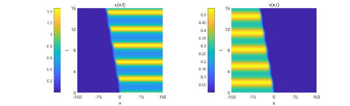
Figure 1: Top views of the $\pi$-periodic bistable wave of (1.1). The coefficient functions are the same as in (5.3). The initial data are $u(x,0)=\frac{0.7660}{1+e^{-x}}$ and $v(x,0)=\frac{0.2977}{1+e^{x}}$.

In Example 2, the coefficient functions are chosen as

$$d_{1}(t)=100,\quad r_{1}(t)=3,\quad\;\;\>a_{1}(t)=3\sin(2t)+14,\quad\;\;\>b_{1}(t)=5\sin(2t)+35;$$ (5.4)

$$d_{2}(t)=120,\quad r_{2}(t)=3.4,\quad a_{2}(t)=1.5\cos(2t)+16,\quad b_{2}(t)=1.5\cos(2t)+6.$$

If we take $s_{0}=0.81$, then we can verify that (1.2) (not (1.6)), and the conditions (4.28) and (4.29) in Theorem 4.2 hold. The dynamical behavior of the $\pi$-periodic bistable traveling wave is displayed in Fig. 2.

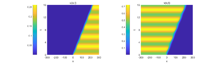
Figure 2: Top views of the $\pi$-periodic bistable wave of (1.1). The coefficient functions are shown in (5.4) and $s_{0}=0.81$. The initial data are $u(x,0)=\frac{0.2378}{1+e^{-x}}$ and $v(x,0)=\frac{0.4779}{1+e^{x}}$.

6 Conclusion and discussion

In this work, we have studied the Lotka-Volterra type of competition model with nonlocal dispersal and time periodicity. By applying the theory of monotone dynamical systems, we prove the existence and monotonicity of the bistable $T$-periodic traveling wave solution. The uniqueness, Lyapunov stability and the value range of the wave speed have been established mainly by means of the comparison principle (the upper and lower solution method). Based on these generic results and the characteristics of the bistable waves, we derive explicit conditions for the speed sign, i.e., Theorems 4.1 and 4.2 guarantee the positive and negative wave speeds, respectively. Moreover, numerical simulations demonstrate our theoretical results even under weak bistable conditions, which reveal the effects of dispersal rate, competition strength, growth rate, seasonality and carrying capacity on the propagation direction of the bistable traveling wave.

It should be pointed out that the monotonicity of the wave speed in terms of the function $b_{1}(t)$ and $a_{2}(t)$ can be easily shown by way of comparison principle. However, a complete classification of the speed sign in terms of all parameters is a challenge. As such, we are particularly interested in obtaining analytic and esay-to-apply formulas for determining the speed sign. Our explicit results are derived by constructing upper/lower solutions with the asymptotical behavior (4.6) which can be seen as case studies, sheding light on further studies and improvement. We expect that different explicit conditions could be obtained by finding different formulas of upper/lower solutions with the asymptotical behaviors similar to (4.8), (4.14) and (4.16), respectively. The exponential stability of the bistable traveling wave of the system (1.1) has been presented in another work. In addition, the condition (1.6) is required only for the existence of traveling waves, while the weaker condition (1.2) (i.e, the bistable condition) is sufficient for other results. Hence we presume that the existence result developed in [7] (i.e., Lemma 2.1) could be improved.

7 Data availability

The simulation code and data are available upon request from the authors. No other data are used.

8 Conflict of interest statement

All authors declare that they have no conflicts of interest.

Acknowledgement. The work of Manjun Ma, Wentao Meng and Jiajun Yue was supported by the National Natural Science Foundation of China (No. 12071434, No. 11671359). The work of Chunhua Ou was supported by the NSERC discovery grants(RGPIN-2016-04709 and RGPIN-2022-03842).

References

- [1] A. Alhasanat and C. Ou, Minimal-speed selection of traveling waves to the Lotka–Volterra competition model, J. Differential Equations, 266 (2019), 7357-7378.
- [2] X. Bao and Z.-C Wang, Existence and stability of time periodic traveling waves for a periodic bistable Lotka-Volterra competition system, J. Differential Equations, 255 (2013), 2402–2435.
- [3] X. Bao, W.-T Li and W. Shen, Traveling wave solutions of Lotka-Volterra competition systems with nonlocal dispersal in periodic habitats, J. Differential Equations, 260 (12) (2016), 8590-8637.
- [4] X. Chen, Existence, uniqueness, and asymptotic stability of traveling waves in nonlocal evolution equations. Adv. Differential Equations, 2 (1997), 125-160.
- [5] C. Conley and R. Gardner, An application of the generalized morse index to travelling wave solutions of a competitive reaction-diffusion model, Indiana Univ. Math. J., 33 (1984), 319–343.
- [6] F.-D. Dong and W.-T. Li, G.-B Zhang, Invasion traveling wave solutions of a predator-prey model with nonlocal dispersal, Commun Nonlinear Sci Numer Simulat, 79 (2019), 104926.
- [7] J. Fang and X.-Q. Zhao, Bistable traveling waves for monotone semiflows with applications, J. Eur. Math. Soc., 17 (2011), 2243–2288.
- [8] J. Fang and X.-Q Zhao, Traveling waves for monotone semiflows with weak compactness, SIAM J. Math. Anal. 46 (6) (2014), 3678-3704.
- [9] R. Gardner, Existence and stability of traveling wave solutions of competition models: a degree theoretic approach, J. Differential Equations, 44 (1982), 343–364.
- [10] L. Girardi and G. Nadin, Travelling waves for diffusive and strongly competitive systems: Relative motility and invasion speed, Euro. Jnl of Applied Mathematics, 26 (2015), 521–534.
- [11] Y. Hosono, Singular perturbation analysis of traveling fronts for the Lotka-Volterra competing models, Numer. Appl. Math., 2 (1989), 687–692.
- [12] Y. Hosono, The minimal speed of traveling fronts for diffusive Lotka-Volterra competition model, Bull. Math. Biol., 60 (1998), 435–448.
- [13] X. Hou, B. Wang and Z.-C. Zhang, The mutual inclusion in a nonlocal competitive Lotka Volterra system, Japan J. Indust. Appl. Math., 31 (2014), 87-110.
- [14] W. Huang, Uniqueness of the bistable traveling wave for mutualist species, J. Dynam. Differential Equations, 13 (2001), 147–183.
- [15] Y. Kan-on, Parameter dependence of propagation speed of traveling waves for competition diffusion equation, SIAM J. Math. Anal., 26 (1995), 340–363.
- [16] Y. Kan-on, Fisher wave fronts for the Lotka-Volterra competition model with diffusion, Nonlinear Anal., 26 (1997), 145–164.
- [17] X.-S. Li and G. Lin, Traveling wavefronts in nonlocal dispersal and cooperative Lotka-Volterra system with delays, Appl. Math. Comput., 204 (2008), 738-744.
- [18] X. Liang, Y. Yi, and X. Q. Zhao, Spreading speeds and traveling waves for periodic evolution systems, J. Differential Equations, 231 (2006), 57–77.
- [19] X. Liang and X.-Q. Zhao, Asymptotic speeds of spread and traveling waves for monotone semiflows with applications, Comm. Pure Appl. Math., 60 (2007), 1-40.
- [20] G. Lin and W.-T. Li, Bistable wavefronts in a diffusive and competitive Lotka-Volterra type system with nonlocal delays, J. Differential Equations, 244 (2008), 487–513.
- [21] M. Ma, Z. Huang, and C. Ou, Speed of the traveling wave for the bistable Lotka-Volterra competition model. Nonlinearity, 32 (2019) 3143-3162.
- [22] S. Pan and G. Lin Invasion traveling wave solutions of a competitive system with dispersal, Bound. Value Probl., 2012 (2012), 1-11.
- [23] Y.-J. Sun and W.-T. Li, Z.-C Wang Traveling waves for a nonlocal anisotropic dispersal equation with monostable nonlinearity, Nonlinear Analysis, 74 (2011), 814-826.
- [24] H. R. Theieme Asymptotic estimates of the solutions of nonlinear integral equations and asymptotic speeds for the spread of poputions, J. Reine Angew. Math, 306 (1979), 94-121.
- [25] Z.-X. Yu, R. Yuan Travelling wave solutions in non-local convolution diffusive competitive-cooperative systems, IMA J Appl Math, 76 (2011), 493-513.
- [26] G.-B. Zhang and R.-Y. Ma, X.-S Li Traveling waves of a Lotka-Volterra strong competition system with nonlocal dispersal, Discrete Contin. Dyn. Syst. Ser. B, 23 (2) (2018), 587-608.
- [27] G.-B. Zhang, W.-T. Li, G. Lin Traveling waves in delayed predator-prey systems with nonlocal diffusion and stage structure, Math Comput Model, 49 (2009), 1021-1029.
- [28] G. Zhao and S. Ruan, Existence, uniqueness and asymptotic stability of time periodic traveling waves for a periodic lotka-volerra competition system with diffusion, J. Math. Pures Appls., 95 (2011), 627–671.