How Does Pseudo-Labeling Affect the Generalization Error of the Semi-Supervised Gibbs Algorithm?

Abstract

We provide an exact characterization of the expected generalization error (gen-error) for semi-supervised learning (SSL) with pseudo-labeling via the Gibbs algorithm. The gen-error is expressed in terms of the symmetrized KL information between the output hypothesis, the pseudo-labeled dataset, and the labeled dataset. Distribution-free upper and lower bounds on the gen-error can also be obtained. Our findings offer new insights that the generalization performance of SSL with pseudo-labeling is affected not only by the information between the output hypothesis and input training data but also by the information shared between the labeled and pseudo-labeled data samples. This serves as a guideline to choose an appropriate pseudo-labeling method from a given family of methods. To deepen our understanding, we further explore two examples—mean estimation and logistic regression. In particular, we analyze how the ratio of the number of unlabeled to labeled data $\lambda$ affects the gen-error under both scenarios. As $\lambda$ increases, the gen-error for mean estimation decreases and then saturates at a value larger than when all the samples are labeled, and the gap can be quantified exactly with our analysis, and is dependent on the cross-covariance between the labeled and pseudo-labeled data samples. For logistic regression, the gen-error and the variance component of the excess risk also decrease as $\lambda$ increases.

1 Introduction

There are several areas, like natural language processing, computer vision, and finance, where labeled data are rare but unlabeled data are abundant. In these situations, semi-supervised learning (SSL) techniques enable us to utilize both labeled and unlabeled data.

Self-training algorithms (Ouali et al., 2020) are a subcategory of SSL techniques. These algorithms use the supervised-learned model’s confident predictions to predict the labels of unlabeled data. Entropy minimization and pseudo-labeling are two basic approaches used in self-training-based SSL. The entropy function may be viewed as a regularization term that penalizes uncertainty in the label prediction of unlabeled data in entropy minimization approaches (Grandvalet et al., 2005). The manifold assumption (Iscen et al., 2019)—where it is assumed that labeled and unlabeled features are drawn from a common data manifold—or the cluster assumption (Chapelle et al., 2003)—where it is assumed that similar data features have a similar label—are assumptions for adopting the entropy minimization algorithm. In contrast, in pseudo-labeling, which is the focus of this work, the model is trained using labeled data and then used to produce a pseudo-label for the unlabeled data (Lee et al., 2013). These pseudo-labels are then utilized to build another model, which is trained using both labeled and pseudo-labeled data in a supervised manner. Studying the generalization error (gen-error) of this procedure is critical to understanding and improving pseudo-labeling performance.

There have been various efforts to characterize the gen-error of SSL algorithms. In Rigollet (2007), an upper bound on the gen-error of binary classification under the cluster assumption is derived. Niu et al. (2013) provides an upper bound on gen-error based on the Rademacher complexity for binary classification with squared-loss mutual information regularization. Göpfert et al. (2019) employs the VC-dimension method to characterize the SSL gen-error. In Göpfert et al. (2019) and Zhu (2020), upper bounds for SSL gen-error using Bayes classifiers are provided. Zhu (2020) also provides an upper bound on the excess risk of SSL algorithm by assuming an exponentially concave function based on the conditional mutual information. He et al. (2022) investigates the gen-error of iterative SSL techniques based on pseudo-labels. An information-theoretic gen-error upper bound on self-training algorithms under the covariate-shift assumption is proposed by Aminian et al. (2022a). These upper bounds on excess risk and gen-error do not entirely capture the impact of SSL, in particular pseudo-labeling and the relative number of labeled and unlabeled data, and thus constrain our ability to fully comprehend the performance of SSL.

In this paper, we are interested in characterizing the expected gen-error of pseudo-labeling-based SSL—using an appropriately-designed Gibbs algorithm—and studying how it depends on the output hypothesis, the labeled, and the pseudo-labeled data. Moreover, we intend to understand the effect of the ratio between the numbers of the unlabeled and labeled training data examples on the gen-error in different scenarios.

Our main contributions in this paper are as follows:

• We provide an exact characterization of the expected gen-error of Gibbs algorithm that models pseudo-labeling-based SSL. This characterization can be applied to obtain novel and informative upper and lower bounds.

• The characterization and bounds offer an insight that reducing the shared information between the labeled and pseudo-labeled samples can help to improve the generalization performance of pseudo-labeling-based SSL.

• We analyze the effect of the ratio of the number of unlabeled data to labeled data $\lambda$ on the gen-error of Gibbs algorithm using a mean estimation example.

• Finally, we study the asymptotic behaviour of the Gibbs algorithm and analyze the effect of $\lambda$ on the gen-error and the excess risk, applying our results to logistic regression.

2 Related Works

Semi-supervised learning: The SSL approaches can be partitioned into six main classes: generative models, low-density separation methods, graph-based methods, self-training and co-training (Zhu, 2008). Among all these, SSL first appeared as self-training in which the model is first trained on the labeled data and annotates the unlabeled data to improve the intial model (Chapelle et al., 2006). SSL has gradually gained more attention after the well-known expectation-minimization (EM) algorithm Moon (1996) was proposed in 1996. One key problem of interest in SSL is whether the unlabeled data can help to improve the performance of learning algorithms. Many existing works have studied this problem either theoretically (e.g., providing bounds) or empirically (e.g., proposing new algorithms). One classical work by Castelli and Cover (1996) set out to study SSL under a traditional setup with unknown mixture of known distributions and characterized the error probability by the fisher information of the labeled and unlabeled data. Szummer and Jaakkola (2002) proposed an algorithm that utilizes the unlabeled data to learn the marginal data distribution to augment learning the class conditional distribution. Amini and Gallinari (2002) empirically showed that semi-supervised logistic regression based on EM algorithm has higher accuracy than the naive Bayes classifier. Singh et al. (2008) studied the benefit of unlabeled data on the excess risk based on the number of unlabeled data and the margin between classes. Ji et al. (2012) developed a simple algorithm based on top eigenfunctions of integral operator derived from both labeled and unlabeled examples that can improve the regression error bound. Li et al. (2019) showed how the unlabeled data can improve the Rademacher-complexity-based generalization error bound of a multi-class classification problem. In deep learning, Berthelot et al. (2019) introduced an effective algorithm that generates low-entropy labels for unlabeled data and then mixes them up with the labeled data to train the model. Sohn et al. (2020) showed that augmenting the confidently pseudo-labeled images can help to improve the accuracy of their model. For a more comprehensive overview of SSL, one can refer to the report by Seeger (2000) and the book by Chapelle et al. (2006).

Pseudo-labeling: Pseudo-labeling is one of the approaches in self-training (Zhu and Goldberg, 2009). Due to the reliance of pseudo-labeling on the quality of the pseudo labels, pseudo-labeling approach might perform poorly. Seeger (2000) stated that there exists a tradeoff between robustness of the learning algorithm and the information gain from the pseudo-labels. Rizve et al. (2020) offered an uncertainty-aware pseudo-labeling strategy to circumvent this difficulty. In Wei et al. (2020), a theoretical framework for combining input-consistency regularization with self-training algorithms in deep neural networks is provided. Dupre et al. (2019) empirically showed that iterative pseudo-labeling with a confidence threshold can improve the test accuracy in early stage. Arazo et al. (2020) showed that the method of generating soft labels for unlabeled data plus mixup augmentation can outperform consistency regularization methods.

Despite the plenty of works on SSL and pseudo-labeling, our work provides a new viewpoint of understanding the effect of pseudo-labeling method on the generalization error using information-theoretic quantities.

Information-theoretic upper bounds: Russo and Zou (2019); Xu and Raginsky (2017) proposed to use the mutual information between the input training set and the output hypothesis to upper bound the expected generalization error. This paves a new way of understanding and improving the generalization performance of a learning algorithm from an information-theoretic viewpoint. Tighter upper bounds by considering the individual sample mutual information is proposed by Bu et al. (2020). Asadi et al. (2018) proposed using chaining mutual information, and Hafez-Kolahi et al. (2020); Haghifam et al. (2020); Steinke and Zakynthinou (2020) advocated the conditioning and processing techniques. Information-theoretic generalization error bounds using other information quantities are also studied, e.g., $f$-divergences, $\alpha$-Rényi divergence and generalized Jensen-Shannon divergence Esposito et al. (2021); Aminian et al. (2022b, 2021b).

3 Semi-Supervised Learning Via The Gibbs Algorithm

In this section, we formulate our problem using the Gibbs algorithm based on both the labeled and unlabeled training data with pseudo-labels. The Gibbs algorithm is a tractable and idealized model for learning algorithms with various approaches, e.g., stochastic optimization methods or relative entropy regularization (Raginsky et al., 2017).

3.1 Problem Formulation

Let $S_{\mathrm{l}}=\{\mathbf{Z}_{i}\}_{i=1}^{n}=\{(\mathbf{X}_{i},Y_{i})\}_{i=1}^{n}$ be the labeled training dataset, where $\mathbf{X}_{i}\in\mathcal{X}=\mathbb{R}^{d}$ is the data feature, $Y_{i}\in\mathcal{Y}=[K]$ is the class label and each pair of $\mathbf{Z}_{i}=(\mathbf{X}_{i},Y_{i})\in\mathcal{X}\times\mathcal{Y}=\mathcal{Z}$ is independently and identically distributed (i.i.d.) from $P_{\mathbf{Z}}=P_{\mathbf{X},Y}\in\mathcal{P}(\mathcal{Z})$. Conditioned on $\mathbf{X}_{i}$, each label $Y_{i}$ is i.i.d. from $P_{Y|\mathbf{X}}$. Let $S_{\mathrm{u}}=\{\mathbf{X}_{i}\}_{i=n+1}^{n+m}$ be the unlabeled training dataset. For all $i\in[n+m]$, each $\mathbf{X}_{i}$ is i.i.d. from $P_{\mathbf{X}}\in\mathcal{P}(\mathcal{X})$. Based on the labeled dataset $S_{\mathrm{l}}$, a pseudo-labeling method assigns a pseudo-label $\hat{Y}_{i}$ to each $\mathbf{X}_{i}\in S_{\mathrm{u}}$ and $\hat{Y}_{i}$ is drawn conditionally i.i.d. from $P_{\hat{Y}|\mathbf{X},S_{\mathrm{l}}}$. Let the pseudo-labeled data point be $\hat{\mathbf{Z}}_{i}=(\mathbf{X}_{i},\hat{Y}_{i})$ and the pseudo-labeled dataset be $\hat{S}_{\mathrm{u}}=\{\hat{\mathbf{Z}}_{i}\}_{i=n+1}^{n+m}$. For any labeled and pseudo-label datasets, we use $P_{S_{\mathrm{l}}}$, $P_{\hat{S}_{\mathrm{u}}}$ and $P_{S_{\mathrm{l}},\hat{S}_{\mathrm{u}}}$ to denote the joint distributions of the data samples in $S_{\mathrm{l}}$, $\hat{S}_{\mathrm{u}}$, and $S_{\mathrm{l}}\cup\hat{S}_{\mathrm{u}}$, respectively. Note that $P_{S_{\mathrm{l}}}=P_{\mathbf{Z}}^{\otimes n}$.

Let $\mathbf{w}\in\mathcal{W}$ denote the output hypothesis. In semi-supervised learning, one considers the empirical risk based on both the labeled and unlabeled data. In this paper, by fixing a mixing weight $\eta\in\mathbb{R}_{+}$, for any loss function $l:\mathcal{W}\times\mathcal{Z}\to\mathbb{R}_{+}$, the total empirical risk is the $\eta$-weighted sum of the empirical risks of the labeled and pseudo-labeled data (McLachlan, 2005; Chapelle et al., 2006)

$$L_{\mathrm{E}}(\mathbf{w},S_{\mathrm{l}},\hat{S}_{\mathrm{u}}):=L_{\mathrm{E}}(\mathbf{w},S_{\mathrm{l}})+\eta L_{\mathrm{E}}(\mathbf{w},\hat{S}_{\mathrm{u}}),$$ (1)

where $L_{\mathrm{E}}(\mathbf{w},S_{\mathrm{l}}):=\frac{1}{n}\sum_{i=1}^{n}l(\mathbf{w},\mathbf{Z}_{i})$ and $L_{\mathrm{E}}(\mathbf{w},\hat{S}_{\mathrm{u}}):=\frac{1}{m}\sum_{i=n+1}^{n+m}l(\mathbf{w},\hat{\mathbf{Z}}_{i})$. Note that, by normalizing the weight $\eta$, minimizing the empirical risk $L_{\mathrm{E}}(\mathbf{w},S_{\mathrm{l}},\hat{S}_{\mathrm{u}})$ is equivalent to minimizing

$$\!\!\bar{L}_{\mathrm{E}}(\mathbf{w},S_{\mathrm{l}},\hat{S}_{\mathrm{u}})\!=\!\frac{1}{1+\eta}L_{\mathrm{E}}(\mathbf{w},S_{\mathrm{l}})\!+\!\frac{\eta}{1+\eta}L_{\mathrm{E}}(\mathbf{w},\hat{S}_{\mathrm{u}}).$$ (2)

The population risk under the true data distribution is

$$L_{\rm P}(\mathbf{w},P_{S_{\mathrm{l}}}):=\mathbb{E}_{S_{\mathrm{l}}\sim P_{S_{\mathrm{l}}}}\big{[}L_{\mathrm{E}}(\mathbf{w},S_{\mathrm{l}})\big{]}.$$ (3)

Under the i.i.d. assumption, such a definition reduces to $\mathbb{E}_{S_{\mathrm{l}}\sim P_{S_{\mathrm{l}}}}\big{[}L_{\mathrm{E}}(\mathbf{w},S_{\mathrm{l}})\big{]}=\mathbb{E}_{\mathbf{Z}\sim P_{\mathbf{Z}}}\big{[}l(\mathbf{w},\mathbf{Z})\big{]}$.

Any SSL algorithm can be characterized by a conditional distribution $P_{\mathbf{W}|S_{\mathrm{l}},\hat{S}_{\mathrm{u}}}$, which is a stochastic map from the labeled dataset $S_{\mathrm{l}}$, the pseudo-labeled dataset $\hat{S}_{\mathrm{u}}$ to the output hypothesis $\mathbf{W}$. For any training datasets $S_{\mathrm{l}},\hat{S}_{\mathrm{u}}$ and any SSL algorithm $P_{\mathbf{W}|S_{\mathrm{l}},\hat{S}_{\mathrm{u}}}$, the expected gen-error is defined as the expected gap between the population risk and the empirical risk of the labeled data $S_{\mathrm{l}}$, i.e.,

$$\overline{\mathrm{gen}}(P_{\mathbf{W}|S_{\mathrm{l}},\hat{S}_{\mathrm{u}}},P_{S_{\mathrm{l}},\hat{S}_{\mathrm{u}}})\!\!:=\!\mathbb{E}_{\mathbf{W},S_{\mathrm{l}}}\![L_{\rm P}(\mathbf{W},P_{S_{\mathrm{l}}})\!\!-\!\!L_{\mathrm{E}}(\mathbf{W},S_{\mathrm{l}})],$$ (4)

which measures the extent to which the algorithm overfits to the labeled training data.

In particular, we consider the Gibbs algorithm (also known as the Gibbs posterior (Catoni, 2007)) to model a pseudo-labeling-based SSL algorithm. Given any $(S_{\mathrm{l}},\hat{S}_{\mathrm{u}})$, the $(\alpha,\pi(\mathbf{w}),\bar{L}_{\mathrm{E}}(\mathbf{w},S_{\mathrm{l}},\hat{S}_{\mathrm{u}}))$-Gibbs algorithm (Gibbs, 1902; Jaynes, 1957) is

$$P_{\mathbf{W}|S_{\mathrm{l}},\hat{S}_{\mathrm{u}}}^{\alpha}(\mathbf{w}|S_{\mathrm{l}},\hat{S}_{\mathrm{u}})=\frac{\pi(\mathbf{w})\exp\big{(}-\alpha\bar{L}_{\mathrm{E}}(\mathbf{w},S_{\mathrm{l}},\hat{S}_{\mathrm{u}})\big{)}}{\Lambda_{\alpha,\eta}(S_{\mathrm{l}},\hat{S}_{\mathrm{u}})},$$

where $\alpha\geq 0$ is the “inverse temperature”, $\Lambda_{\alpha,\eta}(S_{\mathrm{l}},\hat{S}_{\mathrm{u}})\!=\!\int\pi(\mathbf{w})\exp(-\alpha\bar{L}_{\mathrm{E}}(\mathbf{w},S_{\mathrm{l}},\hat{S}_{\mathrm{u}}))\,\mathrm{d}\mathbf{w}$ is the partition function and $\pi(\mathbf{w})$ is the prior of $\mathbf{w}$. We provide more motivations for the Gibbs algorithm model in Appendix A.

Our goal—relying on the characterization of $P_{\mathbf{W}|S_{\mathrm{l}},\hat{S}_{\mathrm{u}}}^{\alpha}$—is to precisely quantify the gen-error in (4) as a function of various information-theoretic quantities.

If $P$ is absolutely continuous with respect to $Q$ and vice versa, let the symmetrized KL-divergence (also known as Jeffrey’s divergence (Jeffreys, 1946)) be defined as $D_{\mathrm{SKL}}(P\|Q):=D(P\|Q)+D(Q\|P)$, where $D$ is the Kullback–Leibler (KL) divergence (Cover, 1999).

For random variables $X$ and $Y$ with joint distribution $P_{X,Y}$, the mutual information is $I(X;Y)=D(P_{X,Y}\|P_{X}\otimes P_{Y})$ and the Lautum information (Palomar and Verdú, 2008) is $L(X;Y)=D(P_{X}\otimes P_{Y}\|P_{X,Y})$. Similarly, the symmetrized KL information between $X$ and $Y$ (Aminian et al., 2015) is defined as $I_{\mathrm{SKL}}(X;Y):=D_{\mathrm{SKL}}(P_{X,Y}\|P_{X}\otimes P_{Y})=I(X;Y)+L(X;Y)$. We define the conditional symmetrized KL information as $I_{\mathrm{SKL}}(X;Y|Z):=I(X;Y|Z)+L(X;Y|Z)$.

3.2 Main Results

One of our main results offers an exact closed-form information-theoretic expression for the gen-error of the $(\alpha,\pi(\mathbf{w}),\bar{L}_{\mathrm{E}}(\mathbf{w},S_{\mathrm{l}},\hat{S}_{\mathrm{u}}))$-Gibbs algorithm in terms of the symmetrized KL information defined above.

Theorem 1.

Under the $(\alpha,\pi(\mathbf{w}),\bar{L}_{\mathrm{E}}(\mathbf{w},S_{\mathrm{l}},\hat{S}_{\mathrm{u}}))$-Gibbs algorithm, the expected gen-error is

$$\overline{\mathrm{gen}}(P_{\mathbf{W}|S_{\mathrm{l}},\hat{S}_{\mathrm{u}}}^{\alpha},P_{S_{\mathrm{l}},\hat{S}_{\mathrm{u}}})\!=\!\frac{1+\eta}{\alpha}\big{(}\mathbb{E}_{\Delta_{S_{\mathrm{l}},\hat{S}_{\mathrm{u}}}}[\log\Lambda_{\alpha,\eta}(S_{\mathrm{l}},\hat{S}_{\mathrm{u}})]$$

$$\quad+I_{\mathrm{SKL}}(\mathbf{W},\hat{S}_{\mathrm{u}};S_{\mathrm{l}})-I_{\mathrm{SKL}}(\hat{S}_{\mathrm{u}};S_{\mathrm{l}})\big{)},$$ (5)

where $\Lambda_{\alpha,\eta}(S_{\mathrm{l}},\hat{S}_{\mathrm{u}}):=\mathbb{E}_{\mathbf{W}\sim\pi}[\exp(-\alpha\bar{L}_{\mathrm{E}}(\mathbf{W},S_{\mathrm{l}},\hat{S}_{\mathrm{u}}))]$ and $\mathbb{E}_{\Delta_{S_{\mathrm{l}},\hat{S}_{\mathrm{u}}}}[\cdot]:=\mathbb{E}_{S_{\mathrm{l}},\hat{S}_{\mathrm{u}}}[\cdot]-\mathbb{E}_{S_{\mathrm{l}}}\mathbb{E}_{\hat{S}_{\mathrm{u}}}[\cdot]$.

The proof of Theorem 1 is provided in Appendix B, where we also show that by letting $\eta\to 0$, the result reduces to that for supervised learning (SL). In addition, we can even extend Theorem 1 to SSL based on other methods, e.g., entropy minimization (Amini and Gallinari, 2002; Grandvalet et al., 2005). This corollary is provided in Section C.

Theorem 1 can also be applied to derive novel bounds on the expected gen-error of the Gibbs algorithm as follows.

Proposition 1.

Assume that the loss function $l(\mathbf{w},\mathbf{Z})$ is bounded in $[a,b]\subset\mathbb{R}_{+}$. Then, the expected gen-error of the $(\alpha,\pi(\mathbf{w}),\bar{L}_{\mathrm{E}}(\mathbf{w},S_{\mathrm{l}},\hat{S}_{\mathrm{u}}))$-Gibbs algorithm satisfies

$$\!\!\left|\overline{\mathrm{gen}}(P_{\mathbf{W}|S_{\mathrm{l}},\hat{S}_{\mathrm{u}}}^{\alpha},P_{S_{\mathrm{l}},\hat{S}_{\mathrm{u}}})\!-\!\text{SKL}\right|\!\leq\!c(\eta,a,b)\sqrt{\!I(\hat{S}_{\mathrm{u}};S_{\mathrm{l}})},$$ (6)

where $c(\eta,a,b):=\frac{1}{\sqrt{2}}(1+\eta)(b-a)$ and $\text{SKL}:=\frac{1+\eta}{\alpha}(I_{\mathrm{SKL}}(\mathbf{W},\hat{S}_{\mathrm{u}};S_{\mathrm{l}})-I_{\mathrm{SKL}}(\hat{S}_{\mathrm{u}};S_{\mathrm{l}}))$.

The proof and more discussions are provided in Appendix D. In fact, we can further explore how the gen-error depends on the information that the output hypothesis contains about the labeled and unlabeled datasets by writing (see Appendix E)

$$I_{\mathrm{SKL}}(\mathbf{W},\hat{S}_{\mathrm{u}};S_{\mathrm{l}})-I_{\mathrm{SKL}}(\hat{S}_{\mathrm{u}};S_{\mathrm{l}})$$

$$=I(\mathbf{W};S_{\mathrm{l}}|\hat{S}_{\mathrm{u}})+D(P_{\mathbf{W}|\hat{S}_{\mathrm{u}}}\|P_{\mathbf{W}|S_{\mathrm{l}},\hat{S}_{\mathrm{u}}}|P_{S_{\mathrm{l}}}P_{\hat{S}_{\mathrm{u}}}).$$ (7)

From Theorem 1 and (3.2), we observe that for any $(\eta,\alpha)$, given $\hat{S}_{\mathrm{u}}$, as the dependency (or the information shared) between $\mathbf{W}$ and $S_{\mathrm{l}}$ decreases, the expected gen-error decreases, and the algorithm is less likely to overfit to the training data. This intuition dovetails with the results for supervised learning in Xu and Raginsky (2017), Russo and Zou (2019) and Aminian et al. (2021a). However, the difference here is that the quantities are conditioned on the pseudo-labeled data $\hat{S}_{\mathrm{u}}$, which reflects the impact of SSL.

Together with Proposition 1, we can observe that the gen-error is also dependent on the information shared between the input labeled and pseudo-labeled data. If the mutual information $I(\hat{S}_{\mathrm{u}};S_{\mathrm{l}})$ decreases, the expected gen-error is likely to decrease as well. This implies that pseudo-labels highly dependent on the labeled dataset may not be beneficial in terms of the generalization performance of an algorithm. In fact, in our subsequent example in Section 4, we exactly quantify the shared information using the cross-covariance between the labeled and pseudo-labeled data. This result sheds light on the future design of pseudo-labeling methods.

3.2.1 Special Cases of Theorem 1

It is instructive to elaborate how Theorem 1 specializes in some well-known learning settings such as transfer learning and SSL not reusing labeled data.

• Case 1 ($\hat{S}_{\mathrm{u}}$ independent of $S_{\mathrm{l}}$): If the pseudo-labels $\{\hat{Y}_{i}\}_{i=n+1}^{n+m}$ are not generated based on the labeled dataset $S_{\mathrm{l}}$, e.g. randomly assigned or generated from another domain (similar to transfer learning), the pseudo-labeled dataset $\hat{S}_{\mathrm{u}}$ is independent of $S_{\mathrm{l}}$. According to the basic properties of mutual and Lautum information (Palomar and Verdú, 2008) and (3.2), we have

  $$I_{\mathrm{SKL}}(\mathbf{W},\hat{S}_{\mathrm{u}};S_{\mathrm{l}})-I_{\mathrm{SKL}}(\hat{S}_{\mathrm{u}};S_{\mathrm{l}})=I_{\mathrm{SKL}}(\mathbf{W};S_{\mathrm{l}}|\hat{S}_{\mathrm{u}}),$$

  and $\mathbb{E}_{\Delta_{S_{\mathrm{l}},\hat{S}_{\mathrm{u}}}}[\log\Lambda_{\alpha,\eta}(S_{\mathrm{l}},\hat{S}_{\mathrm{u}})]=0$. That is,

  $$\!\!\!\overline{\mathrm{gen}}(P_{\mathbf{W}|S_{\mathrm{l}},\hat{S}_{\mathrm{u}}}^{\alpha},P_{S_{\mathrm{l}},\hat{S}_{\mathrm{u}}})\!=\!\frac{(1+\lambda)I_{\mathrm{SKL}}(\mathbf{W};S_{\mathrm{l}}|\hat{S}_{\mathrm{u}})}{\alpha},$$ (8)

  which corresponds to the result of transfer learning in Bu et al. (2022, Theorem 1).

• Case 2 ($S_{\mathrm{l}}-\hat{S}_{\mathrm{u}}-\mathbf{W}$): When this Markov chain holds, meaning that the output hypothesis $\mathbf{W}$ is independent of $S_{\mathrm{l}}$ conditioned on $\hat{S}_{\mathrm{u}}$, we have

  $$I(\mathbf{W};S_{\mathrm{l}}|\hat{S}_{\mathrm{u}})=0,~{}P_{\mathbf{W}|\hat{S}_{\mathrm{u}}}=P_{\mathbf{W}|S_{\mathrm{l}},\hat{S}_{\mathrm{u}}}$$

  $$~{}\text{and}~{}D(P_{\mathbf{W}|\hat{S}_{\mathrm{u}}}\|P_{\mathbf{W}|S_{\mathrm{l}},\hat{S}_{\mathrm{u}}}|P_{S_{\mathrm{l}}}P_{\hat{S}_{\mathrm{u}}})=0.$$

  Thus, the expected gen-error $\overline{\mathrm{gen}}(P_{\mathbf{W}|S_{\mathrm{l}},\hat{S}_{\mathrm{u}}}^{\alpha},P_{S_{\mathrm{l}},\hat{S}_{\mathrm{u}}})=\frac{1+\eta}{\alpha}\mathbb{E}_{\Delta_{S_{\mathrm{l}},\hat{S}_{\mathrm{u}}}}[\log\Lambda_{\alpha,\eta}(S_{\mathrm{l}},\hat{S}_{\mathrm{u}})]$. However, this is a degenerate case. For example, it only occurs when $\eta\to\infty$, i.e., the labeled dataset $S_{\mathrm{l}}$ might be used for generating pseudo-labels for $S_{\mathrm{u}}$ but not used in the Gibbs algorithm to learn the output hypothesis $\mathbf{W}$. In this case, $\overline{\mathrm{gen}}(P_{\mathbf{W}|S_{\mathrm{l}},\hat{S}_{\mathrm{u}}}^{\alpha},P_{S_{\mathrm{l}},\hat{S}_{\mathrm{u}}})=0$.

3.2.2 SSL vs. SL with $n+m$ labeled data

It is also instructive to elaborate on how SSL compares to SL with $n+m$ labeled data based on Theorem 1. In particular, assume that that the labeled training dataset $S_{\mathrm{l}}^{(n+m)}=\{\mathbf{Z}^{\prime}_{i}\}_{i=1}^{n+m}$ contains $n+m$ samples drawn i.i.d. from $P_{\mathbf{Z}}$. Then for any output hypothesis $\mathbf{w}_{\mathrm{SL}}^{(n+m)}\in\mathcal{W}$, the population risk is given by $L_{\mathrm{P}}(\mathbf{w}_{\mathrm{SL}}^{(n+m)},P_{S_{\mathrm{l}}^{(n+m)}})=\mathbb{E}_{\mathbf{Z}^{\prime}\sim P_{\mathbf{Z}}}[l(\mathbf{w}_{\mathrm{SL}}^{(n+m)},\mathbf{Z}^{\prime})]$ (cf. (3)), and the empirical risk of the labeled data samples is given by

$$L_{\mathrm{E}}(\mathbf{w}_{\mathrm{SL}}^{(n+m)},S_{\mathrm{l}}^{(n+m)}) =\frac{1}{n+m}\sum_{i=1}^{n+m}l(\mathbf{w}_{\mathrm{SL}}^{(n+m)},\mathbf{Z}^{\prime}_{i}).$$

From Aminian et al. (2021a, Theorem 1), under the $(\alpha,\pi(\mathbf{w}_{\mathrm{SL}}^{(n+m)}),L_{\mathrm{E}}(\mathbf{w}_{\mathrm{SL}}^{(n+m)},S_{\mathrm{l}}^{(n+m)}))$-Gibbs algorithm, the expected gen-error is

$$\overline{\mathrm{gen}}_{\mathrm{SL}}^{(n+m)} :=\mathbb{E}[L_{\rm P}(\mathbf{W}_{\mathrm{SL}}^{(n+m)},P_{S_{\mathrm{l}}^{(n+m)}})-L_{\mathrm{E}}(\mathbf{W}_{\mathrm{SL}}^{(n+m)},S_{\mathrm{l}}^{(n+m)})]$$

$$=\frac{I_{\mathrm{SKL}}(\mathbf{W}_{\mathrm{SL}}^{(n+m)};S_{\mathrm{l}}^{(n+m)})}{\alpha}.$$ (9)

In the SSL setup, in comparison with (3.2.2), under the $(\alpha,\pi(\mathbf{w}),\bar{L}_{\mathrm{E}}(\mathbf{w},S_{\mathrm{l}},\hat{S}_{\mathrm{u}}))$-Gibbs algorithm, we let the mixing weight $\eta$ of the empirical risk in (2) be the ratio of the number of unlabeled to labeled data, i.e., $\eta=\lambda:=m/n$. We similarly define another expected gen-error $\overline{\mathrm{gen}}_{\mathrm{all}}$ which is also evaluated over $n+m$ data points as follows:

$$\!\overline{\mathrm{gen}}_{\mathrm{all}}(P_{\mathbf{W}|S_{\mathrm{l}},\hat{S}_{\mathrm{u}}}^{\alpha},P_{S_{\mathrm{l}},\hat{S}_{\mathrm{u}}})\!:=\!\mathbb{E}[L_{\rm P}(\mathbf{W},P_{S_{\mathrm{l}}})\!-\!L_{\mathrm{E}}(\mathbf{W},S_{\mathrm{l}},\hat{S}_{\mathrm{u}})].$$

Consider the situation where the pseudo-labeling method is perfect such that $P_{\hat{Y}_{i}|\mathbf{X}_{i}}=P_{Y|\mathbf{X}}$ for all $i\in[n+1:n+m]$. Then any $\hat{\mathbf{Z}}_{i}\in\hat{S}_{\mathrm{u}}$ has the same distribution as that of any $\mathbf{Z}\in S_{\mathrm{l}}$. By applying the same technique in the proof of Theorem 1, we obtain (details provided in Appendix F)

$$\overline{\mathrm{gen}}_{\mathrm{all}}(P_{\mathbf{W}|S_{\mathrm{l}},\hat{S}_{\mathrm{u}}}^{\alpha},P_{S_{\mathrm{l}},\hat{S}_{\mathrm{u}}})=\frac{I_{\mathrm{SKL}}(\mathbf{W};S_{\mathrm{l}},\hat{S}_{\mathrm{u}})}{\alpha}.$$ (10)

However, only when $P_{\hat{Y}_{i}|\mathbf{X}_{i},S_{\mathrm{l}}}=P_{\hat{Y}_{i}|\mathbf{X}_{i}}=P_{Y|\mathbf{X}}$ for any $S_{\mathrm{l}}$, $I_{\mathrm{SKL}}(\mathbf{W};S_{\mathrm{l}},\hat{S}_{\mathrm{u}})=I_{\mathrm{SKL}}(\mathbf{W}_{\mathrm{SL}}^{(n+m)};S_{\mathrm{l}}^{(n+m)})$ and $\overline{\mathrm{gen}}_{\mathrm{all}}=\overline{\mathrm{gen}}_{\mathrm{SL}}^{(n+m)}$; otherwise, the gen-errors of SL in (3.2.2) and of SSL in (10) may not be equal. This is because the pseudo-label $\hat{Y}_{i}$’s are assumed to be generated based on the labeled dataset $S_{\mathrm{l}}$ and this dependence affects the gen-error. As we have discussed following Proposition 1, if the information shared between $S_{\mathrm{l}}$ and $\hat{S}_{\mathrm{u}}$ is large, the learning algorithm tends to overfit to the labeled training data.

If the $\hat{Y}_{i}$’s are independent of $S_{\mathrm{l}}$, then $P_{\hat{Y}_{i}|\mathbf{X}_{i},S_{\mathrm{l}}}=P_{\hat{Y}_{i}|\mathbf{X}_{i}}$ for any $S_{\mathrm{l}}$. Consider the situation where the pseudo-labeling method is close to perfect, i.e., $P_{\hat{\mathbf{Z}}}=P_{\mathbf{Z}}+\epsilon\Delta$, where $\epsilon>0$ is small and $\int_{\mathcal{Z}}\Delta(\mathbf{z})\mathrm{d}\mathbf{z}=0$ such that $P_{\hat{\mathbf{Z}}}\geq 0$. We have

$$\overline{\mathrm{gen}}_{\mathrm{all}}(P_{\mathbf{W}|S_{\mathrm{l}},\hat{S}_{\mathrm{u}}}^{\alpha},P_{S_{\mathrm{l}},\hat{S}_{\mathrm{u}}})\!=\!\frac{I_{\mathrm{SKL}}(\mathbf{W}_{\mathrm{SL}}^{(n+m)};S_{\mathrm{l}}^{(n+m)})}{\alpha}\!+\!\tilde{\epsilon},$$

where $\tilde{\epsilon}$ is proportional to $\epsilon$ and $\tilde{\epsilon}\to 0$ as $\epsilon\to 0$ (details are provided in Appendix F.2). Therefore, in this special case, we see that the gap between $\overline{\mathrm{gen}}_{\mathrm{all}}$ of SSL and $\overline{\mathrm{gen}}_{\mathrm{SL}}^{(n+m)}$ of SL can be directly quantified by the gap between the labeled and pseudo-labeled distributions.

3.3 Distribution-Free Upper and Lower Bounds

We can also build upon Theorem 1 and Xu and Raginsky (2017, Theorem 1) to provide distribution-free upper and lower bounds of the gen-error in (5). We next state an informal version of such bounds (the formal version and the proof are provided in Appendix G). Throughout this section, we let the mixing weight $\eta=\lambda=m/n$.

Proposition 2 (Informal Version).

Assume $I(\hat{S}_{\mathrm{u}};S_{\mathrm{l}})=\gamma_{\alpha,\lambda}I(\mathbf{W},\hat{S}_{\mathrm{u}};S_{\mathrm{l}})$, for some $\gamma_{\alpha,\lambda}\in[0,1]$ that depends on $\lambda$ and $\alpha$. Assume that $l(\mathbf{w},\mathbf{Z})$ is bounded in $[a,b]\subset\mathbb{R}_{+}$. Let $\gamma^{\prime}_{\alpha,\lambda,a,b}=\frac{\alpha(b-a)^{2}\sqrt{\gamma_{\alpha,\lambda}}}{2(1-\gamma_{\alpha,\lambda})}$. Then the expected gen-error can be bounded as follows

$$\!\!-\gamma^{\prime}_{\alpha,\lambda,a,b}\!\bigg{(}\frac{1}{\sqrt{n}}\!+\!\frac{\sqrt{\gamma_{\alpha,\lambda}}}{1+\lambda}\bigg{)}\leq\overline{\mathrm{gen}}(P_{\mathbf{W}|S_{\mathrm{l}},\hat{S}_{\mathrm{u}}}^{\alpha},P_{S_{\mathrm{l}},\hat{S}_{\mathrm{u}}})\leq\gamma^{\prime}_{\alpha,\lambda,a,b}\bigg{(}\frac{1}{\sqrt{n}}+\frac{1}{(n+m)\sqrt{\gamma_{\alpha,\lambda}}}\bigg{)}.$$ (11)

Recall that for SL with $n$ labeled data, the expected gen-error is of order $O(\frac{1}{n})$ Aminian et al. (2021a, Theorem 2). This can be naturally extended to SL with $n+m$ labeled data, leading to the expected gen-error behaving as $O(\frac{1}{n+m})$. Compared to the SL case, we see that using the pseudo-labeled data may degrade the convergence rate of the expected gen-error and the extent to which it degrades depends on $\gamma_{\alpha,\lambda}$, which captures the impact of the amount of information shared among the output hypothesis, the input labeled and unlabeled data as well as the ratio $\lambda$. If $\gamma_{\alpha,\lambda}$ is small, it implies $I(\hat{S}_{\mathrm{u}};S_{\mathrm{l}})$ is small and $I(\mathbf{W};S_{\mathrm{l}}|\hat{S}_{\mathrm{u}})$ is large, which leads to a tight upper bound.

If we fix $0<\lambda<\infty$ and assume $\hat{S}_{\mathrm{u}}$ is independent of $S_{\mathrm{l}}$, then $\gamma_{\alpha,\lambda}=0$ and

$$0\leq\overline{\mathrm{gen}}(P_{\mathbf{W}|S_{\mathrm{l}},\hat{S}_{\mathrm{u}}}^{\alpha},P_{S_{\mathrm{l}},\hat{S}_{\mathrm{u}}})\leq\frac{\alpha(b-a)^{2}}{2(n+m)},$$

which coincides with the result of transfer learning in Bu et al. (2022, Remark 3) and corresponds to the analysis of (8). Although it appears that using independent pseudo-labeled data $\hat{S}_{\mathrm{u}}$ does not degrade the convergence rate of the expected gen-error, it may affect the excess risk or the test accuracy, which taken in unison, represents the performance of a learning algorithm. The definition and further analysis of the excess risk is provided in Section 5.1.1.

When $\lambda\to 0$, the gen-error converges to that of SL with $n$ labeled data and the distribution-free upper bound is of order $O(\frac{1}{n})$, given in Aminian et al. (2021a, Theorem 2).

4 An Application to Mean Estimation

To deepen our understanding of the expected gen-error in Theorem 1, we study a mean estimation example and analyze how $\lambda=m/n$ affects the gen-error.

4.1 Problem Setup

For any $(\mathbf{X}_{i},Y_{i})\in S_{\mathrm{l}}$ and $i\in[n]$, we assume that $Y_{i}\in\{-1,+1\}$, $\mathbb{E}[\mathbf{X}_{i}|Y_{i}=1]=\bm{\mu}$, $\mathbb{E}[\mathbf{X}_{i}|Y_{i}=-1]=-\bm{\mu}$, $\|\bm{\mu}\|_{2}=1$ and $\operatorname{Cov}[Y_{i}\mathbf{X}_{i}]=\sigma^{2}\mathbf{I}_{d}$. Any $\mathbf{X}\in S_{\mathrm{u}}$ is drawn i.i.d. from the same distribution as $\mathbf{X}_{i}$. Consider the problem of learning $\bm{\mu}$ using $S_{\mathrm{l}}$ and $\hat{S}_{\mathrm{u}}$. We adopt the mean-squared loss $l(\mathbf{w},\mathbf{z})=\|\mathbf{w}-y\mathbf{x}\|_{2}^{2}$ and assume the prior $\pi(\mathbf{w})$ is uniform on $\mathcal{W}$. Based on $\mathbf{W}_{0}$ learned from the labeled dataset $S_{\mathrm{l}}$ (e.g., $\mathbf{W}_{0}=\frac{1}{n}\sum_{i=1}^{n}Y_{i}\mathbf{X}_{i}$), we assign a pseudo-label to each $X_{i}\in S_{\mathrm{u}}$ as $\hat{Y}_{i}$ (e.g. $\hat{Y}_{i}=\operatorname{sgn}(\mathbf{W}_{0}^{\top}\mathbf{X}_{i})$) and let $\bm{\mu}^{\prime}=\mathbb{E}[\hat{Y}_{i}\mathbf{X}_{i}]$. Let us construct $S_{\mathrm{l}}^{\prime}=\{Y_{i}\mathbf{X}_{i}\}_{i=1}^{n}$ and $\hat{S}_{\mathrm{u}}^{\prime}=\{\hat{Y}_{i}\mathbf{X}_{i}\}_{i=n+1}^{n+m}$. The empirical risk is given by (cf. (2) by replacing $S_{\mathrm{l}},\hat{S}_{\mathrm{u}}$ with $S_{\mathrm{l}}^{\prime},\hat{S}_{\mathrm{u}}^{\prime}$)

$$\bar{L}_{\mathrm{E}}(\mathbf{w},S_{\mathrm{l}}^{\prime},\hat{S}_{\mathrm{u}}^{\prime}) =\frac{1}{(1+\lambda)n}\sum_{i=1}^{n}\|Y_{i}\mathbf{X}_{i}-\mathbf{w}\|_{2}^{2}+\frac{\lambda}{(1+\lambda)m}\sum_{j=n+1}^{n+m}\|\hat{Y}_{j}\mathbf{X}_{j}-\mathbf{w}\|_{2}^{2}.$$

The expected gen-error is equal to the right-hand side of (5) by replacing $S_{\mathrm{l}},\hat{S}_{\mathrm{u}}$ with $S_{\mathrm{l}}^{\prime},\hat{S}^{\prime}_{\mathrm{u}}$.

The $(\alpha,\pi(\mathbf{W}),\bar{L}_{\mathrm{E}}(\mathbf{W},S_{\mathrm{l}}^{\prime},\hat{S}_{\mathrm{u}}^{\prime}))$-Gibbs algorithm is given by the following Gibbs posterior distribution

$$P_{\mathbf{W}|S_{\mathrm{l}}^{\prime},\hat{S}_{\mathrm{u}}^{\prime}}^{\alpha}(\mathbf{W}|S_{\mathrm{l}}^{\prime},\hat{S}^{\prime}_{\mathrm{u}})=\mathcal{N}(\bm{\mu}_{n+m},\sigma^{2}_{\mathrm{l},\mathrm{u}}\mathbf{I}_{d}),$$

where $\sigma^{2}_{\mathrm{l},\mathrm{u}}=\frac{1}{2\alpha}$ and

$$\!\bm{\mu}_{n,m}\!=\!\frac{1}{(1+\lambda)n}\sum_{i=1}^{n}Y_{i}\mathbf{X}_{i}+\frac{\lambda}{(1+\lambda)m}\sum_{j=n+1}^{n+m}\hat{Y}_{j}\mathbf{X}_{j}.$$

Details are provided in Appendix H. With this posterior Gaussian distribution $P_{\mathbf{W}|S_{\mathrm{l}}^{\prime},\hat{S}_{\mathrm{u}}^{\prime}}^{\alpha}$, the expected gen-error in Theorem 1 can be exactly computed as follows

$$\!\!\overline{\mathrm{gen}}(P_{\mathbf{W}|S_{\mathrm{l}},\hat{S}_{\mathrm{u}}}^{\alpha},P_{S_{\mathrm{l}},\hat{S}_{\mathrm{u}}})=\frac{2\sigma^{2}d}{n+m}+\frac{2m}{n+m}\mathbb{E}\big{[}(Y_{i}\mathbf{X}_{i}-\bm{\mu})^{\top}(\hat{Y}_{j}\mathbf{X}_{j}-\bm{\mu}^{\prime})\big{]},$$ (12)

where $i\in[n]$ and $j\in[n+1:n+m]$ run over the labeled and unlabeled datasets respectively. From the definition of the expected gen-error in (4), we obtain the same result, which corroborates the characterization of the expected gen-error in Theorem 1. See Appendix H for details.

Note that the second term in (12) is the trace of the cross-covariance between the labeled and pseudo-labeled data sample, i.e., for any $i\in[n]$ and $j\in[n+1:n+m]$,

$$\!\mathbb{E}\big{[}(Y_{i}\mathbf{X}_{i}-\bm{\mu})^{\top}(\hat{Y}_{j}\mathbf{X}_{j}-\bm{\mu}^{\prime})\big{]}\!=\!\operatorname{tr}(\operatorname{Cov}[Y_{i}\mathbf{X}_{i},\hat{Y}_{j}\mathbf{X}_{j}]).$$

This result shows that for any fixed $(n,m)$, the expected gen-error decreases when the trace of the cross-covariance decreases, which corroborates our analyses in Section 3.2.

4.2 Effect of the Pseudo-labeling and the Ratio of Unlabeled to Labeled Samples $\lambda$

To futher study the effect of the pseudo-labeling method and the ratio $\lambda=m/n$, in this mean estimation example, we consider the class-conditional feature distribution of $\mathbf{X}_{i}|Y_{i}\sim\mathcal{N}(Y_{i}\bm{\mu},\sigma^{2}\mathbf{I}_{d})$ for any $i\in[n+m]$. Let $S_{\mathrm{l}}^{\prime(n+m)}$ be a dataset with $n+m$ independent copies of $Y\mathbf{X}\in S_{\mathrm{l}}^{\prime}$. Similarly to (12), for the supervised $(\alpha,\pi(\mathbf{w}_{\mathrm{SL}}^{(n)}),L_{\mathrm{E}}(\mathbf{w}_{\mathrm{SL}}^{(n)},S_{\mathrm{l}}^{\prime}))$-Gibbs algorithm and the supervised $(\alpha,\pi(\mathbf{w}_{\mathrm{SL}}^{(n+m)}),L_{\mathrm{E}}(\mathbf{w}_{\mathrm{SL}}^{(n+m)},S_{\mathrm{l}}^{\prime(n+m)}))$-Gibbs algorithm, the expected gen-errors are respectively given by (see details in Appendix H.1)

$$\overline{\mathrm{gen}}_{\mathrm{SL}}^{(n)}=\frac{2\sigma^{2}d}{n}\quad\mbox{and}\quad\overline{\mathrm{gen}}_{\mathrm{SL}}^{(n+m)}=\frac{2\sigma^{2}d}{n+m}.$$

Let $\overline{\mathrm{gen}}_{\mathrm{SSL}}$ denote $\overline{\mathrm{gen}}(P_{\mathbf{W}|S_{\mathrm{l}},\hat{S}_{\mathrm{u}}}^{\alpha},P_{S_{\mathrm{l}},\hat{S}_{\mathrm{u}}})$ for brevity. By comparing $\overline{\mathrm{gen}}_{\mathrm{SL}}^{(n)}$ and $\overline{\mathrm{gen}}_{\mathrm{SL}}^{(n+m)}$, we observe that:

1. If $\mathbb{E}\big{[}(Y_{i}\mathbf{X}_{i}-\bm{\mu})^{\top}(\hat{Y}_{j}\mathbf{X}_{j}-\bm{\mu}^{\prime})\big{]}<0$, then $\overline{\mathrm{gen}}_{\mathrm{SSL}}<\overline{\mathrm{gen}}_{\mathrm{SL}}^{(n+m)}$, which means that SSL with such pseudo-labeling method even has better generalization performance than SL with $n+m$ labeled data. This is the most desirable case in terms of the generalization error;

2. If $\mathbb{E}\big{[}(Y_{i}\mathbf{X}_{i}-\bm{\mu})^{\top}(\hat{Y}_{j}\mathbf{X}_{j}-\bm{\mu}^{\prime})\big{]}>\frac{\sigma^{2}d}{n}$, then $\overline{\mathrm{gen}}_{\mathrm{SSL}}>\overline{\mathrm{gen}}_{\mathrm{SL}}^{(n)}$. This implies that if the cross-covariance between the labeled and pseudo-labeled data is larger than a certain threshold, the pseudo-labeling method does not help to improve the generalization performance;

3. If $0\leq\mathbb{E}\big{[}(Y_{i}\mathbf{X}_{i}-\bm{\mu})^{\top}(\hat{Y}_{j}\mathbf{X}_{j}-\bm{\mu}^{\prime})\big{]}\leq\frac{\sigma^{2}d}{n}$, then $\overline{\mathrm{gen}}_{\mathrm{SL}}^{(n+m)}\leq\overline{\mathrm{gen}}_{\mathrm{SSL}}\leq\overline{\mathrm{gen}}_{\mathrm{SL}}^{(n)}$. This implies that if the cross-covariance is sufficiently small, pseudo-labeling improves the generalization error.

The value of $\mathbb{E}\big{[}(Y_{i}\mathbf{X}_{i}-\bm{\mu})^{\top}(\hat{Y}_{j}\mathbf{X}_{j}-\bm{\mu}^{\prime})\big{]}$ also depends on the ratio $\lambda$. Next, to study the effect of $\lambda$, let the initial hypothesis learned from the labeled data $S_{\mathrm{l}}$ be $\mathbf{W}_{0}=\frac{1}{n}\sum_{i=1}^{n}Y_{i}\mathbf{X}_{i}\sim\mathcal{N}(\bm{\mu},\frac{\sigma^{2}}{n}\mathbf{I}_{d})$ and the pseudo-label for any $\mathbf{X}_{i}\in S_{\mathrm{u}}$ be $\hat{Y}_{i}=\operatorname{sgn}(\mathbf{W}_{0}^{\top}\mathbf{X}_{i})$.

Inspired by the derivation techniques in He et al. (2022), we can rewrite the expected gen-error in (12) as

$$\overline{\mathrm{gen}}(P_{\mathbf{W}|S_{\mathrm{l}},\hat{S}_{\mathrm{u}}}^{\alpha},P_{S_{\mathrm{l}},\hat{S}_{\mathrm{u}}})=\frac{2\sigma^{2}d}{n+m}+\frac{2m}{n+m}E_{n},$$ (13)

where $E_{n}=\mathbb{E}[\tilde{g}J_{\sigma}(\gamma_{n}^{\prime})+\|\bm{\mu}^{\perp}\|_{2}K_{\sigma}(\gamma_{n}^{\prime})]$, $\tilde{g}\sim\mathcal{N}(0,1)$, $\bm{\mu}^{\perp}\sim\mathcal{N}(\textbf{0},\mathbf{I}_{d}-\bm{\mu}\bm{\mu}^{\top})$, $J_{\sigma}$ and $K_{\sigma}$ are functions with domain $[-1,1]$, and $\gamma_{n}^{\prime}\in[-1,1]$ is a sequence of correlation coefficients. Details are presented in Appendix H.2, where we also prove that $E_{n}=O(d)$ and $E_{n}\geq 0$, which means that we always have $\overline{\mathrm{gen}}_{\mathrm{SL}}^{(n+m)}\leq\overline{\mathrm{gen}}_{\mathrm{SSL}}$ here. Furthermore, we observe that $E_{n}$ does not depend on $m$ and thus, (13) converges to $2E_{n}$ when we fix $n$, and let $\lambda\to\infty$.

In Figure 1, we numerically plot $\overline{\mathrm{gen}}_{\mathrm{SSL}}$ by varying $\lambda$ and compare it with $\overline{\mathrm{gen}}_{\mathrm{SL}}^{(n)}$ and $\overline{\mathrm{gen}}_{\mathrm{SL}}^{(n+m)}$ for different values of noise level $\sigma$, and number of labeled data samples $n$. Under different choices of $\sigma$, we observe that $\overline{\mathrm{gen}}_{\mathrm{SL}}^{(n+m)}\leq\overline{\mathrm{gen}}_{\mathrm{SSL}}\leq\overline{\mathrm{gen}}_{\mathrm{SL}}^{(n)}$. Moreover, the gen-error of SSL monotonically decreases as $\lambda$ increases, showing obvious improvement compared to $\overline{\mathrm{gen}}_{\mathrm{SL}}^{(n)}$. However, there exists a gap $\frac{2\lambda E_{n}}{1+\lambda}$ between $\overline{\mathrm{gen}}_{\mathrm{SSL}}$ and $\overline{\mathrm{gen}}_{\mathrm{SL}}^{(n+m)}$. For $n$ large enough (e.g., $n=100$) or noise level small enough (e.g., $\sigma=0.5$), this gap is almost negligible, which means pseudo-labeling yields comparable generalization performance as the SL when all the samples are labeled.

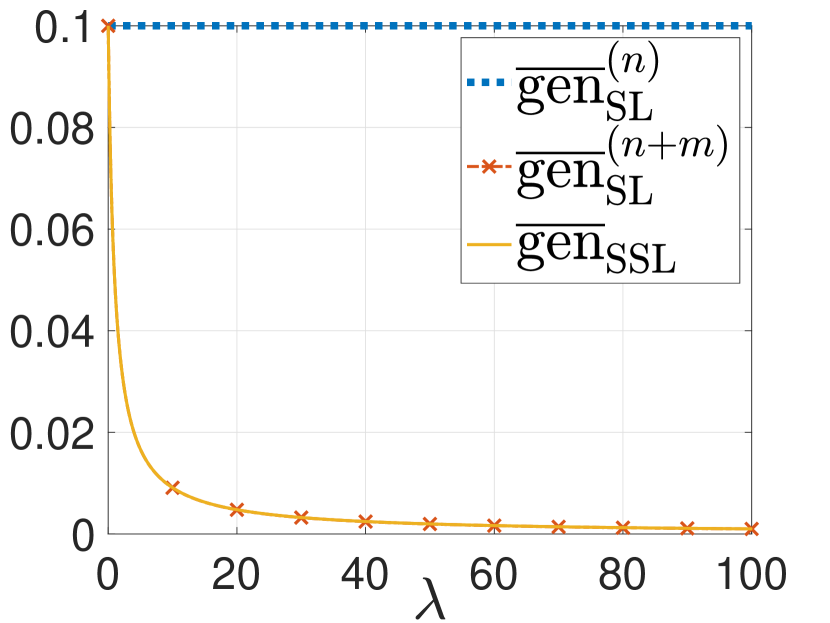
(a) $\sigma=0.5$, $n=5$

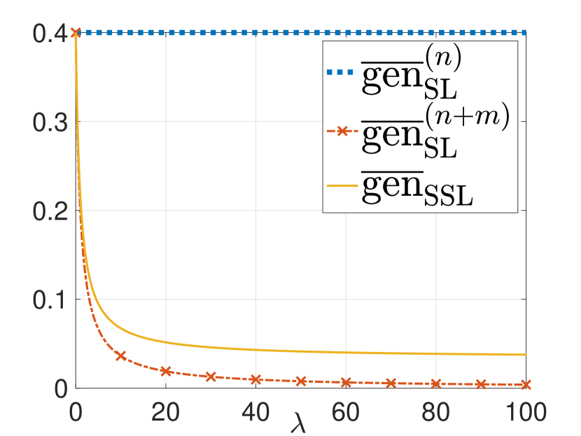
(b) $\sigma=1$, $n=5$

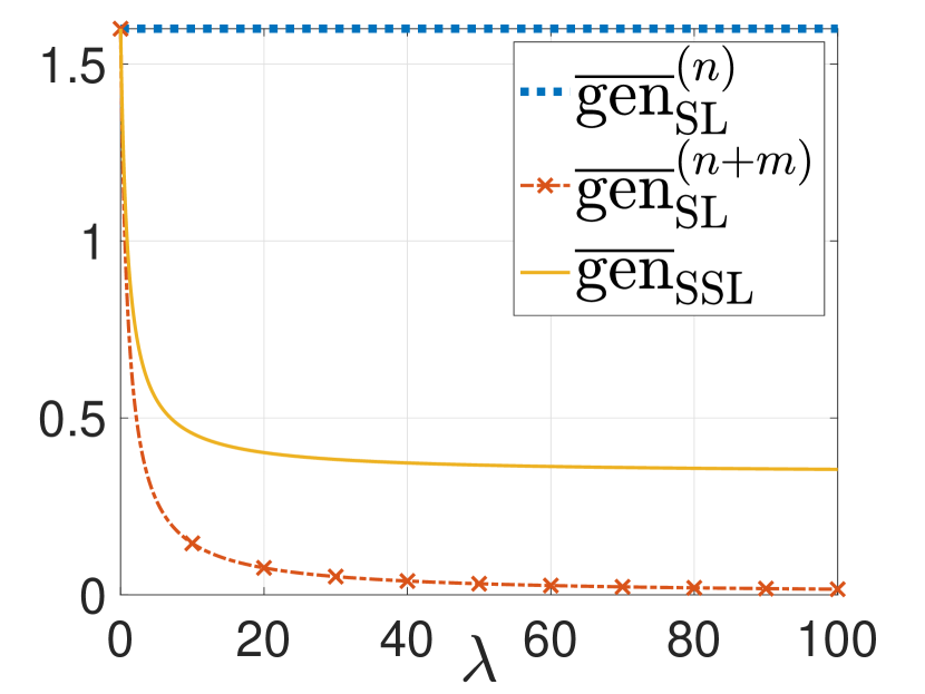
(c) $\sigma=2$, $n=5$

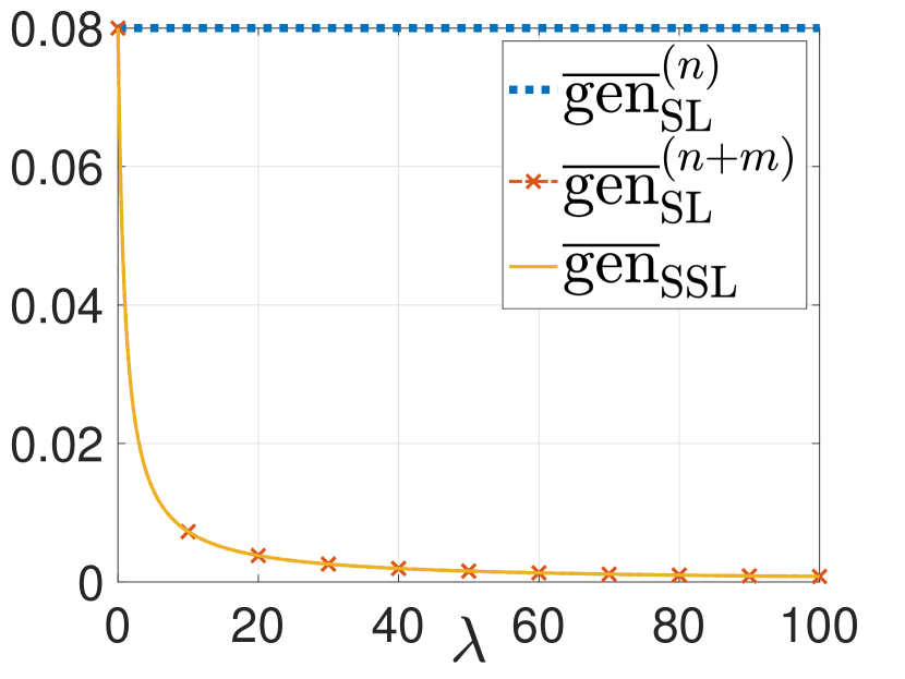
(d) $\sigma=2$, $n=100$

Figure 1: Gen-error of mean estimation vs.  $\lambda=m/n$.

4.3 Choosing a Pseudo-labeling Method from a Given Family of Methods

We have shown that the generalization error decreases as the information shared between the input labeled and pseudo-labeled data (represented by the mutual information $I(\hat{S}_{\mathrm{u}};S_{\mathrm{l}})$ or the cross-covariance term $\operatorname{tr}(\operatorname{Cov}[Y_{i}\mathbf{X}_{i},\hat{Y}_{j}\mathbf{X}_{j}])$ in the mean estimation example) decreases. This result serves as a guideline for choosing an appropriate pseudo-labeling method. For example, if we are given a set of pseudo-labeling functions $\{f_{i}\}_{i=1}^{C}$ with $f_{i}:\mathcal{X}\to\mathcal{Y}$, we can choose the best one $f_{i^{*}}$ that yields the minimum mutual information $I(\hat{S}_{\mathrm{u}};S_{\mathrm{l}})$. To make our ideas more concrete, for the mean estimation example that we have been discussing thus far, assume that the pseudo-labeling functions $\hat{Y}=\operatorname{sgn}(\mathbf{W}_{0}^{\top}\mathbf{X})\mathbf{1}_{\{|\mathbf{W}_{0}^{\top}\mathbf{X}|\geq T\}}$ (where $\mathbf{X}\in S_{\mathrm{u}}$) are indexed by various “confidence” thresholds $T\in\mathbb{R}_{+}$ ($T$ plays the role of the index $i$ in $\{f_{i}\}_{i=1}^{C}$). For instance, let us consider the case where $n=5$, $\sigma=1$ (cf. Figure 1(b)). As shown in Figure 2, one can choose the threshold $T$ that minimizes $\operatorname{tr}(\operatorname{Cov}[Y_{i}\mathbf{X}_{i},\hat{Y}_{j}\mathbf{X}_{j}])$ for $(\mathbf{X}_{i},Y_{i})\in S_{\mathrm{l}}$ and $\mathbf{X}_{j}\in S_{\mathrm{u}}$. From this figure, we observe that $T\geq 7$ approximately minimizes $\operatorname{tr}(\operatorname{Cov}[Y_{i}\mathbf{X}_{i},\hat{Y}_{j}\mathbf{X}_{j}])$ and hence, the generalization error. We have thus exhibited a concrete way to choose one pseudo-labeling method from a given family of methods via our characterization of generalization error.

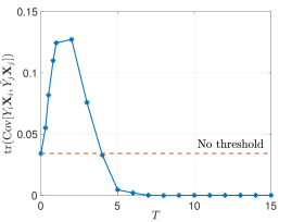
Figure 2: The cross-covariance term between labelled and pseudo-labelled data for different confidence threshold $T$.

5 Particularizing The Gibbs Algorithm To Empirical Risk Minimization

In this section, we consider the asymptotic behavior of the expected gen-error and excess risk for the Gibbs algorithm under SSL as the “inverse temperature” $\alpha\to\infty$. It is known that the Gibbs algorithm converges to empirical risk minimization (ERM) as $\alpha\to\infty$; see Appendix A.

Given any $S_{\mathrm{l}},\hat{S}_{\mathrm{u}}$, assume that there exists a unique minimizer of the empirical risk $\bar{L}_{\mathrm{E}}(\mathbf{W},S_{\mathrm{l}},\hat{S}_{\mathrm{u}})$ (also known as the single-well case), i.e.,

$$\mathbf{W}^{*}(S_{\mathrm{l}},\hat{S}_{\mathrm{u}})=\operatorname*{arg\,min}_{\mathbf{w}\in\mathcal{W}}\bar{L}_{\mathrm{E}}(\mathbf{w},S_{\mathrm{l}},\hat{S}_{\mathrm{u}}).$$

Let the Hessian matrix of the empirical risk $\bar{L}_{\mathrm{E}}(\mathbf{w},S_{\mathrm{l}},\hat{S}_{\mathrm{u}})$ at $\mathbf{w}=\mathbf{W}^{*}(S_{\mathrm{l}},\hat{S}_{\mathrm{u}})$ be defined as

$$H^{*}(S_{\mathrm{l}},\hat{S}_{\mathrm{u}})=\nabla_{\mathbf{w}}^{2}\bar{L}_{\mathrm{E}}(\mathbf{w},S_{\mathrm{l}},\hat{S}_{\mathrm{u}})|_{\mathbf{w}=\mathbf{W}^{*}(S_{\mathrm{l}},\hat{S}_{\mathrm{u}})}.$$

Under the single-well case, we obtain a characterization of the asymptotic expected gen-error in the following theorem.

Theorem 2.

Under the $(\alpha,\pi(\mathbf{w}),\bar{L}_{\mathrm{E}}(\mathbf{w},S_{\mathrm{l}},\hat{S}_{\mathrm{u}}))$-Gibbs algorithm, as $\alpha\to\infty$, if the Hessian matrix $H^{*}(S_{\mathrm{l}},\hat{S}_{u})$ is not singular and $\mathbf{W}^{*}(S_{\mathrm{l}},\hat{S}_{\mathrm{u}})$ is unique, the expected gen-error converges to

$$\overline{\mathrm{gen}}(P_{\mathbf{W}|S_{\mathrm{l}},\hat{S}_{\mathrm{u}}}^{\infty},P_{S_{\mathrm{l}},\hat{S}_{\mathrm{u}}})$$

$$=\mathbb{E}_{\hat{S}_{\mathrm{u}},S_{\mathrm{l}}}\Big{[}\mathbf{W}^{*}(S_{\mathrm{l}},\hat{S}_{\mathrm{u}})^{\top}H^{*}(S_{\mathrm{l}},\hat{S}_{\mathrm{u}})\mathbf{W}^{*}(S_{\mathrm{l}},\hat{S}_{\mathrm{u}})\Big{]}$$

$$\quad+\mathbb{E}_{\hat{S}_{\mathrm{u}}}\mathbb{E}_{S_{\mathrm{l}}}\Big{[}\Big{(}\mathbf{W}^{*}(S_{\mathrm{l}},\hat{S}_{\mathrm{u}})-2\mathbb{E}_{S_{\mathrm{l}}|\hat{S}_{\mathrm{u}}}[\mathbf{W}^{*}(S_{\mathrm{l}},\hat{S}_{\mathrm{u}})]\Big{)}^{\top}\cdot H^{*}(S_{\mathrm{l}},\hat{S}_{\mathrm{u}})\mathbf{W}^{*}(S_{\mathrm{l}},\hat{S}_{\mathrm{u}})\Big{]}$$

$$\quad-\mathbb{E}_{\Delta_{S_{\mathrm{l}},\hat{S}_{\mathrm{u}}}}\Big{[}\bar{L}_{\mathrm{E}}(\mathbf{W}^{*}(S_{\mathrm{l}},\hat{S}_{\mathrm{u}}),S_{\mathrm{l}},\hat{S}_{\mathrm{u}})\Big{]}-\mathbb{E}_{\Delta_{(\mathbf{W},\hat{S}_{\mathrm{u}}),S_{\mathrm{l}}}}\Big{[}\mathbf{W}^{\top}H^{*}(S_{\mathrm{l}},\hat{S}_{\mathrm{u}})\mathbf{W}\Big{]}\bigg{)},$$ (14)

where the expectations $\mathbb{E}_{\Delta_{S_{\mathrm{l}},\hat{S}_{\mathrm{u}}}}[\cdot]:=\mathbb{E}_{S_{\mathrm{l}},\hat{S}_{\mathrm{u}}}[\cdot]-\mathbb{E}_{S_{\mathrm{l}}}\mathbb{E}_{\hat{S}_{\mathrm{u}}}[\cdot]$ and $\mathbb{E}_{\Delta_{(\mathbf{W},\hat{S}_{\mathrm{u}}),S_{\mathrm{l}}}}[\cdot]:=\mathbb{E}_{\mathbf{W},\hat{S}_{\mathrm{u}},S_{\mathrm{l}}}[\cdot]-\mathbb{E}_{\mathbf{W},\hat{S}_{\mathrm{u}}}\mathbb{E}_{S_{\mathrm{l}}}[\cdot]$.

The proof of Theorem 2 is provided in Appendix I. Theorem 2 shows that the gen-error of the Gibbs algorithm under SSL when $\alpha\to\infty$ depends strongly on the second derivatives of the empirical risk (a.k.a. loss landscape) and the relationship between $S_{\mathrm{l}}$ and $\hat{S}_{\mathrm{u}}$. The loss landscape is an important tool to understand the dynamics of the learning process in deep learning. In the extreme case where $S_{\mathrm{l}}$ and $\hat{S}_{\mathrm{u}}$ are independent, $\mathbb{E}_{\Delta_{S_{\mathrm{l}},\hat{S}_{\mathrm{u}}}}\big{[}\bar{L}_{\mathrm{E}}(\mathbf{W}^{*}(S_{\mathrm{l}},\hat{S}_{\mathrm{u}}),S_{\mathrm{l}},\hat{S}_{\mathrm{u}})\big{]}=0$ and a simplified expression for the asymptotic gen-error is provided in Appendix J.

5.1 Semi-Supervised Maximum Likelihood Estimation

In particular, by letting the loss function be the negative log-likelihood, this algorithm becomes semi-supervised maximum likelihood estimation (SS-MLE). In this part, we consider the SS-MLE in the asymptotic regime where $n,m\to\infty$. Throughout this section, we let the mixing weight in (2) $\eta=\lambda=m/n$.

We aim to fit the training data with a parametric family $p(\cdot|\mathbf{w})$, where $\mathbf{w}\in\mathcal{W}$. Consider the negative log-loss function $l(\mathbf{w},\mathbf{z})=-\log p(\mathbf{z}|\mathbf{w})$. For the single-well case, the unique minimizer is

$$\mathbf{W}^{*}(S_{\mathrm{l}},\hat{S}_{\mathrm{u}})=\operatorname*{arg\,min}_{\mathbf{w}\in\mathcal{W}}\bigg{(}-\frac{1}{1+\lambda}\cdot\frac{1}{n}\sum_{i=1}^{n}\log p(\mathbf{Z}_{i}|\mathbf{w})-\frac{\lambda}{1+\lambda}\cdot\frac{1}{m}\sum_{i=n+1}^{n+m}\log p(\hat{\mathbf{Z}}_{i}|\mathbf{w})\bigg{)}.$$ (15)

Given any labeled dataset $S_{\mathrm{l}}$, we use $P_{\hat{\mathbf{Z}}|S_{\mathrm{l}}}=\mathbb{E}_{\mathbf{W}_{0}|S_{\mathrm{l}}}[P_{\hat{\mathbf{Z}}|\mathbf{W}_{0}}]$ to denote the conditional distribution of the pseudo-labeled data (i.e., $\hat{\mathbf{Z}}_{i}\overset{\text{i.i.d.}}{\sim}P_{\hat{\mathbf{Z}}|S_{\mathrm{l}}}$), where $\mathbf{W}_{0}$ is the initial hypothesis learned only from $S_{\mathrm{l}}$ and used to generate pseudo-labels for $S_{\mathrm{u}}$. Assume that $\mathbf{W}_{0}$ is learned from $S_{\mathrm{l}}$ using MLE, i.e.,

$$\mathbf{W}_{0}=\operatorname*{arg\,min}_{\mathbf{w}\in\mathcal{W}}-\frac{1}{n}\sum_{i=1}^{n}\log p(\mathbf{Z}_{i}|\mathbf{w}).$$

We have $\mathbf{W}_{0}\xrightarrow{\mathrm{p}}\mathbf{w}^{*}_{P_{\mathbf{Z}}}=\operatorname*{arg\,min}_{\mathbf{w}\in\mathcal{W}}D(P_{\mathbf{Z}}\|p(\cdot|\mathbf{w}))$ as $n\to\infty$, where $\mathbf{w}^{*}_{P_{\mathbf{Z}}}$ depends only on the true distribution of the labeled data $P_{\mathbf{Z}}$. Then we have $P_{\hat{\mathbf{Z}}|\mathbf{W}_{0}}\xrightarrow{\mathrm{p}}P_{\hat{\mathbf{Z}}|\mathbf{w}^{*}_{P_{\mathbf{Z}}}}$, $P_{\hat{\mathbf{Z}}|S_{\mathrm{l}}}\xrightarrow{\mathrm{p}}P_{\hat{\mathbf{Z}}|\mathbf{w}^{*}_{P_{\mathbf{Z}}}}$ and $P_{\hat{\mathbf{Z}}}=\mathbb{E}_{\mathbf{W}_{0}}[P_{\hat{\mathbf{Z}}|\mathbf{W}_{0}}]\xrightarrow{\mathrm{p}}P_{\hat{\mathbf{Z}}|\mathbf{w}^{*}_{P_{\mathbf{Z}}}}$, which means $\{\hat{\mathbf{Z}}_{i}\}_{i=n+1}^{n+m}$ become independent of one another and of $S_{\mathrm{l}}$. We analogously define the minimizer

$$\mathbf{w}^{*}_{\lambda}= \operatorname*{arg\,min}_{\mathbf{w}\in\mathcal{W}}\bigg{(}\frac{n}{n+m}D\big{(}P_{\mathbf{Z}}\|p(\cdot|\mathbf{w})\big{)}+\frac{m}{n+m}D\big{(}P_{\hat{\mathbf{Z}}|\mathbf{w}^{*}_{P_{\mathbf{Z}}}}\|p(\cdot|\mathbf{w})\big{)}\bigg{)}$$ (16)

and the landscapes of the loss function

$$J_{\mathrm{l}}(\mathbf{w}) :=\mathbb{E}_{\mathbf{Z}\sim P_{\mathbf{Z}}}[-\nabla_{\mathbf{w}}^{2}\log p(\mathbf{Z}|\mathbf{w})],$$

$$J_{\mathrm{u}}(\mathbf{w}) :=\mathbb{E}_{\hat{\mathbf{Z}}\sim P_{\hat{\mathbf{Z}}|\mathbf{w}^{*}_{P_{\mathbf{Z}}}}}[-\nabla_{\mathbf{w}}^{2}\log p(\hat{\mathbf{Z}}|\mathbf{w})],$$

$$\mathcal{I}_{\mathrm{l}}(\mathbf{w}) :=\mathbb{E}_{\mathbf{Z}\sim P_{\mathbf{Z}}}[\nabla_{\mathbf{w}}\log p(\mathbf{Z}|\mathbf{w})\nabla_{\mathbf{w}}\log p(\mathbf{Z}|\mathbf{w})^{\top}].$$

Let $J(\mathbf{w})=\frac{n}{n+m}J_{\mathrm{l}}(\mathbf{w})+\frac{m}{n+m}J_{\mathrm{u}}(\mathbf{w})$. Given any ratio $\lambda>0$, as $n,m\to\infty$, by the law of large numbers, the Hessian matrix $H^{*}(S_{\mathrm{l}},\hat{S}_{\mathrm{u}})$ converges as follows

$$H^{*}(S_{\mathrm{l}},\hat{S}_{\mathrm{u}})\xrightarrow{\mathrm{p}}J(\mathbf{w}^{*}_{\lambda}),$$

which is independent of $(S_{\mathrm{l}},\hat{S}_{\mathrm{u}})$. Leveraging these asymptotic approximations, from Theorem 2, we obtain the following characterization of the gen-error of SS-MLE.

Corollary 1.

In the asymptotic regime where $n,m\to\infty$, the expected gen-error of SS-MLE is given by

$$\overline{\mathrm{gen}}(P_{\mathbf{W}|S_{\mathrm{l}},\hat{S}_{\mathrm{u}}}^{\infty},P_{S_{\mathrm{l}},\hat{S}_{\mathrm{u}}})=\frac{\operatorname{tr}(J(\mathbf{w}^{*}_{\lambda})^{-1}\mathcal{I}_{\mathrm{l}}(\mathbf{w}^{*}_{\lambda}))}{n+m}.$$

The proof of Corollary 1 is provided in Appendix J. For the extreme cases where $\lambda\to 0$, we have $\mathbf{w}^{*}_{\lambda}\to\mathbf{w}^{*}_{P_{\mathbf{Z}}}$, $J(\mathbf{w}^{*}_{\lambda})\to J_{\mathrm{l}}(\mathbf{w}^{*}_{P_{\mathbf{Z}}})$ and $\!\overline{\mathrm{gen}}(P_{\mathbf{W}|S_{\mathrm{l}},\hat{S}_{\mathrm{u}}}^{\infty},P_{S_{\mathrm{l}},\hat{S}_{\mathrm{u}}})\!\!\to\!\!\frac{1}{n}\operatorname{tr}(J_{\mathrm{l}}(\mathbf{w}^{*}_{P_{\mathbf{Z}}})^{-1}\mathcal{I}_{\mathrm{l}}(\mathbf{w}^{*}_{P_{\mathbf{Z}}}))\!=\!O(\frac{d}{n}),$ which means the gen-error degenerates to that of the SL case with $n$ labeled data.

For the other case where $\lambda\to\infty$, from Appendix J, we have $\mathbf{W}_{\mathrm{ML}}(S_{\mathrm{l}},\hat{S}_{\mathrm{u}})\to\mathbb{E}_{S_{\mathrm{l}}}[\mathbf{W}_{\mathrm{ML}}(S_{\mathrm{l}},\hat{S}_{\mathrm{u}})]$ and $\overline{\mathrm{gen}}(P_{\mathbf{W}|S_{\mathrm{l}},\hat{S}_{\mathrm{u}}}^{\infty},P_{S_{\mathrm{l}},\hat{S}_{\mathrm{u}}})\to 0.$

For $\lambda\!\in\!(0,\infty)$, we have $\overline{\mathrm{gen}}(P_{\mathbf{W}|S_{\mathrm{l}},\hat{S}_{\mathrm{u}}}^{\infty},P_{S_{\mathrm{l}},\hat{S}_{\mathrm{u}}})\!=\!O(\frac{d}{n+m})$, which is order-wise the same as the gen-error of SL with $n+m$ labeled data. The intuition is that for large $n$, the pseudo-labeled samples only depend on the labeled data distribution instead of the labeled samples. However, the performance of an algorithm depends not only on the gen-error and but also on the excess risk. Even when the gen-error is small, the bias of the excess risk may be high.

5.1.1 Excess Risk as $\alpha,n,m\to\infty$

In this section, we discuss the excess risk of SS-MLE when $n,m\to\infty$. The excess risk is defined as the gap between the expectation and the minimum of the population risk, i.e.,

$$\mathcal{E}_{\mathrm{r}}(P_{\mathbf{W}}) :=\mathbb{E}_{\mathbf{W}}[L_{\mathrm{P}}(\mathbf{W},P_{S_{\mathrm{l}}})]-L_{\mathrm{P}}(\mathbf{w}_{\mathrm{l}}^{*},P_{S_{\mathrm{l}}})$$ (17)

$$=\overline{\mathrm{gen}}(P_{\mathbf{W}|S_{\mathrm{l}},\hat{S}_{\mathrm{u}}}^{\alpha},P_{S_{\mathrm{l}},\hat{S}_{\mathrm{u}}})+\mathbb{E}_{\mathbf{W},S_{\mathrm{l}}}[L_{\mathrm{E}}(\mathbf{W},S_{\mathrm{l}})-L_{\mathrm{E}}(\mathbf{w}_{\mathrm{l}}^{*},S_{\mathrm{l}})].$$ (18)

where $\mathbf{w}_{\mathrm{l}}^{*}=\operatorname*{arg\,min}_{\mathbf{w}\in\mathcal{W}}L_{\mathrm{P}}(\mathbf{W},P_{S_{\mathrm{l}}})$ is the optimal hypothesis. The second term in (18) is known as the estimation error. We observe that the excess risk depends on both the gen-error and estimation error. When the gen-error is controlled to be sufficiently small, but if the estimation error is large, the excess risk can still be large.

Corollary 2.

In the asymptotic regime where $n,m\to\infty$, the excess risk of SS-MLE is given by

$$\!\!\mathcal{E}_{\mathrm{r}}(P_{\mathbf{W}})=\frac{1}{2}\operatorname{tr}((\mathbf{w}^{*}_{\lambda}-\mathbf{w}^{*}_{\mathrm{l}})(\mathbf{w}^{*}_{\lambda}-\mathbf{w}^{*}_{\mathrm{l}})^{\top}J_{\mathrm{l}}(\mathbf{w}_{\mathrm{l}}^{*}))+\frac{\operatorname{tr}(J_{\mathrm{l}}(\mathbf{w}_{\mathrm{l}}^{*})J(\mathbf{w}^{*}_{\lambda})^{-1}\mathcal{I}_{\mathrm{l}}(\mathbf{w}^{*}_{\lambda})J(\mathbf{w}^{*}_{\lambda})^{-1})}{2(1+\lambda)(n+m)}.$$ (19)

The proof of Corollary 2 is provided in Appendix K. In (19), the first term represents the bias caused by learning with the mixture of labeled and pseudo-labeled data. When $\lambda\to 0$, the bias converges to $0$. As $\lambda$ increases, the bias increases. The second term represents the variance component of the excess risk, which is of order $O(\frac{d}{m+n})$ for $0<\lambda<\infty$, the same as that for the gen-error in Corollary 1.

5.2 An Application to Logistic Regression

To re-emphasize, we let the mixing weight in (2) $\eta=\lambda=m/n$. We now apply SS-MLE to logistic regression to study the effect of $\lambda$ on the gen-error and excess risk. For any hypothesis $\mathbf{w}$, let $p(y|\mathbf{x},\mathbf{w})$ be the conditional likelihood of a label upon seeing a feature sample under $\mathbf{w}$. Assume that the label $Y\in\{-1,+1\}$. For any $\mathbf{z}\in\mathcal{X}\times\{-1,+1\}$, the underlying distribution is $P_{\mathbf{Z}}(\mathbf{z})=P_{Y|\mathbf{X}}(y|\mathbf{x})P_{\mathbf{X}}(\mathbf{x})$ and the logistic regression model uses $p(y|\mathbf{x},\mathbf{w})$ to approximate $P_{Y|\mathbf{X}}(y|\mathbf{x})$. Let $P_{\mathbf{Z}|\mathbf{w}}(\mathbf{z}|\mathbf{w})=p(y|\mathbf{x},\mathbf{w})P_{\mathbf{X}}(\mathbf{x})$. To stabilize the solution $\mathbf{w}$, we consider a regularized version of the logistic regression model, where for a fixed $\nu>0$, the objective function can be expressed as

$$l(\mathbf{w},\mathbf{z}) =-\log p(y|\mathbf{x},\mathbf{w})+\frac{\nu}{2}\|\mathbf{w}\|_{2}^{2}=\log(1+e^{-y\mathbf{w}^{\top}\mathbf{x}})+\frac{\nu}{2}\|\mathbf{w}\|_{2}^{2}.$$

We assume that there exists a unique minimizer of the empirical risk in this example. We also assume that the initial hypothesis $\mathbf{W}_{0}$ is learned from the labeled dataset $S_{\mathrm{l}}$:

$$\mathbf{W}_{0}=\operatorname*{arg\,min}_{\mathbf{w}\in\mathcal{W}}\bigg{(}\frac{1}{n}\sum_{i=1}^{n}\log(1+e^{-Y_{i}\mathbf{w}^{\top}\mathbf{X}_{i}})+\frac{\nu}{2}\|\mathbf{w}\|_{2}^{2}\bigg{)}.$$

Consider the case when $n,m\to\infty$ and $\lambda>0$. Then

$$\mathbf{W}_{0}\!\xrightarrow{\mathrm{p}}\!\mathbf{w}^{*}_{0}\!=\!\operatorname*{arg\,min}_{\mathbf{w}\in\mathcal{W}}\!\bigg{(}\!D\bigg{(}P_{\mathbf{Z}}\bigg{\|}\frac{P_{\mathbf{X}}}{1+e^{-Y\mathbf{w}^{\top}\mathbf{X}}}\bigg{)}\!+\!\frac{\nu}{2}\|\mathbf{w}\|_{2}^{2}\!\bigg{)}.$$

Let the pseudo label for any $\mathbf{X}_{i}\in S_{\mathrm{u}}$ be defined as $\hat{Y}_{i}=\operatorname{sgn}(\mathbf{X}_{i}^{\top}\mathbf{W}_{0})$. The conditional distribution of the pseudo-labeled data sample given $\mathbf{W}_{0}$ converges as follows

$$\!\!P_{\hat{\mathbf{Z}}|\mathbf{W}_{0}}(\hat{\mathbf{z}}|\mathbf{W}_{0})\!\!\xrightarrow{\mathrm{p}}\!\!P_{\hat{\mathbf{Z}}|\mathbf{w}^{*}_{0}}(\hat{\mathbf{z}}|\mathbf{w}^{*}_{0})\!=\!P_{\mathbf{X}}(\mathbf{x})\!\mathbbm{1}\{\hat{y}\!=\!\operatorname{sgn}(\mathbf{x}^{\top}\mathbf{w}^{*}_{0})\!\}.$$

Let us rewrite the minimizer $\mathbf{w}^{*}_{\lambda}$ in (16) as

$$\mathbf{w}^{*}_{\lambda}= \operatorname*{arg\,min}_{\mathbf{w}\in\mathcal{W}}\bigg{(}\frac{n}{n+m}D\big{(}P_{\mathbf{Z}}\|p(\cdot|\mathbf{w})\big{)}+\frac{m}{n+m}D\big{(}P_{\hat{\mathbf{Z}}|\mathbf{w}^{*}_{0}}\|p(\cdot|\mathbf{w})\big{)}+\frac{\nu}{2}\|\mathbf{w}\|_{2}^{2}\bigg{)}.$$

Recall the expected gen-error in Corollary 1, which can also be rewritten as

$$n\cdot\overline{\mathrm{gen}}(P_{\mathbf{W}|S_{\mathrm{l}},\hat{S}_{\mathrm{u}}}^{\infty},P_{S_{\mathrm{l}},\hat{S}_{\mathrm{u}}})\!=\!\frac{\operatorname{tr}((J(\mathbf{w}^{*}_{\lambda})+\nu\mathbf{I}_{d})^{-1}\mathcal{I}_{\mathrm{l}}(\mathbf{w}^{*}_{\lambda}))}{1+\lambda}.$$

Details of the derivation are provided in Appendix L. We focus on the right-hand side, which depends on the ratio $\lambda$ instead of the individual $m,n$. As mentioned in Section 5.1, when $\lambda\to 0$, $n\cdot\overline{\mathrm{gen}}(P_{\mathbf{W}|S_{\mathrm{l}},\hat{S}_{\mathrm{u}}}^{\infty},P_{S_{\mathrm{l}},\hat{S}_{\mathrm{u}}})\to d$. On the other hand, the excess risk $\mathcal{E}_{\mathrm{r}}(P_{\mathbf{W}})$ of this example is given by Corollary 2 where $J(\mathbf{w}^{*}_{\lambda})$ is replaced by $J(\mathbf{w}^{*}_{\lambda})+\nu\mathbf{I}_{d}$. Intuitively, as the regularization parameter $\nu$ increases, the gen-error decreases.

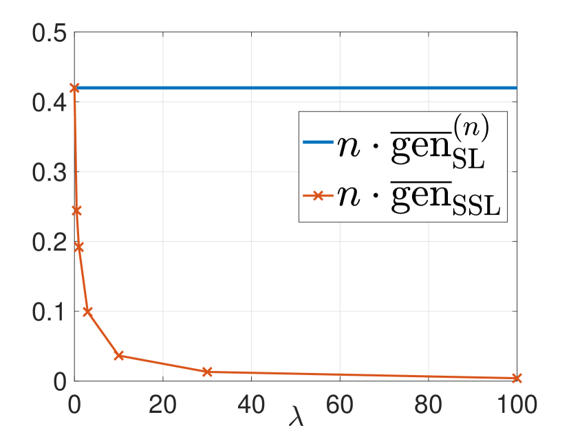
(a) Theoretical gen-error

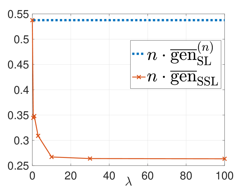
(b) Empirical gen-error

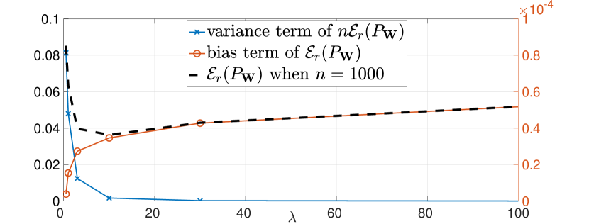
(c) Theoretical excess risk

Figure 3: Theoretical and empirical gen-error and excess risk vs. $\lambda=m/n$ when $\mu=2$ and $\nu=0.001$.

For different values of $\lambda$, we can numerically calculate the hypothesis $\mathbf{w}^{*}_{\lambda}$, the expected gen-error and the excess risk. Consider the example of a dataset which contains two classes of Gaussian samples. Let $P_{\mathbf{X}|Y}=\mathcal{N}(Y\mu\mathbf{1}_{d},\mathbf{I}_{d})$ and $P_{Y}=\mathrm{Unif}(\{-1,+1\})$, where $\mu\in\mathbb{R}_{+}$ and $\mathbf{1}_{d}$ is the all-ones vector in $\mathbb{R}^{d}$. For notational simplicity, let $\overline{\mathrm{gen}}_{\mathrm{SSL}}$ denote $\overline{\mathrm{gen}}(P_{\mathbf{W}|S_{\mathrm{l}},\hat{S}_{\mathrm{u}}}^{\infty},P_{S_{\mathrm{l}},\hat{S}_{\mathrm{u}}})$. In Figure 3, we plot $n\cdot\overline{\mathrm{gen}}_{\mathrm{SSL}}$ and $\mathcal{E}_{\mathrm{r}}(P_{\mathbf{W}})$ versus $\lambda$ when $\mu=2$ and $d=2$. We also implement experiments ($n=1,000$) for $40$ times on synthetic data and plot the average empirical gen-error for $\lambda\in\{0,0.5,1,3,10,30,100\}$. In both theoretical and empirical plots, we observe that as the ratio $\lambda$ increases, the gen-error of SSL decreases and is smaller than that of SL with only $n$ labeled data. We also observe similar behaviours of the empirical gen-error of logistic regression on MNIST dataset (see Appendix L). On the other hand, the variance component of the excess risk behaves similarly as the gen-error while the bias component increases. By taking $n=1,000$, we can see the excess risk first decreases and then increases as $\lambda$ increases. In this setting, our results suggest that when $\lambda$ exceeds some threshold, it may not be beneficial to the performance of the learning algorithm by utilizing any more unlabeled data.

6 Concluding Remarks

To develop a comprehensive understanding of SSL, we present an exact characterization of the expected gen-error of pseudo-labeling-based SSL via the Gibbs algorithm. Our results reveal that the expected gen-error is influenced by the information shared between the labeled and pseudo-labeled data and the ratio of the number of unlabeled data to labeled data. This sheds light in our quest to design good pseudo-labeling methods, which should penalize the dependence between the labeled and pseudo-labeled data, e.g., $I(\hat{S}_{\mathrm{u}};S_{\mathrm{l}})$, so as to improve the generalization performance. To understand the ERM counterpart of pseudo-labeling-based SSL, we also investigate the asymptotic regime, in which the inverse temperature $\alpha\to\infty$. Finally, we present two examples—mean estimation and logistic regression—as applications of our theoretical findings.

Appendix A Motivations for Gibbs Algorithm

There are different motivations for the Gibbs algorithm as discussed in Raginsky et al. (2017); Kuzborskij et al. (2019); Asadi and Abbe (2020); Aminian et al. (2021a). Following are an overview of the most prominent motivations for the Gibbs algorithm:

Empirical Risk Minimization: The $(\alpha,\pi(\mathbf{W}),\bar{L}_{\mathrm{E}}(\mathbf{W},S_{\mathrm{l}},\hat{S}_{\mathrm{u}}))$-Gibbs algorithm can be viewed as a randomized version of empirical risk minimization (ERM). As the inverse temperature $\alpha\to\infty$, then hypothesis generated by the Gibbs algorithm converges to the hypothesis corresponding to standard ERM.

SGLD Algorithm: As discussed in Chiang et al. (1987) and Markowich and Villani (2000), the Stochastic Gradient Langevin Dynamics (SGLD) algorithm can be viewed as the discrete version of the continuous-time Langevin diffusion, and it is defined as follows:

$$\mathbf{W}_{k+1}=\mathbf{W}_{k}-\beta\,\nabla\bar{L}_{\mathrm{E}}(\mathbf{W}_{k},S_{\mathrm{l}},\hat{S}_{\mathrm{u}})+\sqrt{\frac{2\beta}{\gamma}}\,\zeta_{k},\quad k=0,1,\cdots,$$ (20)

where $\zeta_{k}$ is a standard Gaussian random vector and $\beta>0$ is the step size. In Raginsky et al. (2017), it is proved that under some conditions on the loss function, the conditional distribution $P_{\mathbf{W}_{k}|S_{\mathrm{l}},\hat{S}_{\mathrm{u}}}$ induced by SGLD algorithm is close to the $(\gamma,\pi(\mathbf{W}_{0}),\bar{L}_{\mathrm{E}}(\mathbf{W}_{k},S_{\mathrm{l}},\hat{S}_{\mathrm{u}}))$-Gibbs distribution in 2-Wasserstein distance for sufficiently large iterations, $k$.

Appendix B Proof of Theorem 1

Under the $(\alpha,\pi(\mathbf{W}),\bar{L}_{\mathrm{E}}(\mathbf{W},S_{\mathrm{l}},\hat{S}_{\mathrm{u}}))$-Gibbs algorithm, we have

$$I_{\mathrm{SKL}}(\mathbf{W},\hat{S}_{\mathrm{u}};S_{\mathrm{l}})$$

$$=\mathbb{E}_{\mathbf{W},\hat{S}_{\mathrm{u}},S_{\mathrm{l}}}[\log P_{\mathbf{W}|S_{\mathrm{l}},\hat{S}_{\mathrm{u}}}^{\alpha}+\log P_{\hat{S}_{\mathrm{u}}|S_{\mathrm{l}}}]-\mathbb{E}_{\mathbf{W},\hat{S}_{\mathrm{u}}}\mathbb{E}_{S_{\mathrm{l}}}[\log P_{\mathbf{W}|S_{\mathrm{l}},\hat{S}_{\mathrm{u}}}^{\alpha}+\log P_{\hat{S}_{\mathrm{u}}|S_{\mathrm{l}}}]$$ (21)

$$=\mathbb{E}_{\mathbf{W},\hat{S}_{\mathrm{u}},S_{\mathrm{l}}}[-\alpha\bar{L}_{\mathrm{E}}(\mathbf{W},S_{\mathrm{l}},\hat{S}_{\mathrm{u}})-\log\Lambda_{\alpha,\eta}(S_{\mathrm{l}},\hat{S}_{\mathrm{u}})]-\mathbb{E}_{\mathbf{W},\hat{S}_{\mathrm{u}}}\mathbb{E}_{S_{\mathrm{l}}}[-\alpha\bar{L}_{\mathrm{E}}(\mathbf{W},S_{\mathrm{l}},\hat{S}_{\mathrm{u}})-\log\Lambda_{\alpha,\eta}(S_{\mathrm{l}},\hat{S}_{\mathrm{u}})]$$

$$\quad+\mathbb{E}_{\hat{S}_{\mathrm{u}},S_{\mathrm{l}}}[\log P_{\hat{S}_{\mathrm{u}}|S_{\mathrm{l}}}]-\mathbb{E}_{\hat{S}_{\mathrm{u}}}\mathbb{E}_{S_{\mathrm{l}}}[\log P_{\hat{S}_{\mathrm{u}}|S_{\mathrm{l}}}]$$ (22)

$$=\frac{\alpha}{1+\eta}(\mathbb{E}_{\mathbf{W}}[L_{\mathrm{P}}(\mathbf{W},P_{S_{\mathrm{l}}})]-\mathbb{E}_{\mathbf{W},S_{\mathrm{l}}}[L_{\mathrm{E}}(\mathbf{W},S_{\mathrm{l}})])+\mathbb{E}_{\hat{S}_{\mathrm{u}},S_{\mathrm{l}}}[\log P_{\hat{S}_{\mathrm{u}}|S_{\mathrm{l}}}]-\mathbb{E}_{\hat{S}_{\mathrm{u}}}\mathbb{E}_{S_{\mathrm{l}}}[\log P_{\hat{S}_{\mathrm{u}}|S_{\mathrm{l}}}]$$

$$\quad-\mathbb{E}_{\hat{S}_{\mathrm{u}},S_{\mathrm{l}}}[\log\Lambda_{\alpha,\eta}(S_{\mathrm{l}},\hat{S}_{\mathrm{u}})]+\mathbb{E}_{\hat{S}_{\mathrm{u}}}\mathbb{E}_{S_{\mathrm{l}}}[\log\Lambda_{\alpha,\eta}(S_{\mathrm{l}},\hat{S}_{\mathrm{u}})]$$ (23)

$$=\frac{\alpha}{1+\eta}\overline{\mathrm{gen}}(P_{\mathbf{W}|S_{\mathrm{l}},\hat{S}_{\mathrm{u}}},P_{S_{\mathrm{l}},\hat{S}_{\mathrm{u}}})+I_{\mathrm{SKL}}(\hat{S}_{\mathrm{u}};S_{\mathrm{l}})-\mathbb{E}_{\Delta_{S_{\mathrm{l}},\hat{S}_{\mathrm{u}}}}[\log\Lambda_{\alpha,\eta}(S_{\mathrm{l}},\hat{S}_{\mathrm{u}})],$$ (24)

where $\Lambda_{\alpha,\eta}(S_{\mathrm{l}},\hat{S}_{\mathrm{u}})=\int\pi(\mathbf{w})\exp(-\alpha\bar{L}_{\mathrm{E}}(\mathbf{w},S_{\mathrm{l}},\hat{S}_{\mathrm{u}}))\mathrm{d}\mathbf{w}$ and $\mathbb{E}_{\Delta_{S_{\mathrm{l}},\hat{S}_{\mathrm{u}}}}[\cdot]=\mathbb{E}_{S_{\mathrm{l}},\hat{S}_{\mathrm{u}}}[\cdot]-\mathbb{E}_{S_{\mathrm{l}}}\mathbb{E}_{\hat{S}_{\mathrm{u}}}[\cdot]$.

Thus, the expected gen-error is given by

$$\overline{\mathrm{gen}}(P_{\mathbf{W}|S_{\mathrm{l}},\hat{S}_{\mathrm{u}}},P_{S_{\mathrm{l}},\hat{S}_{\mathrm{u}}})=\frac{(1+\eta)(I_{\mathrm{SKL}}(\mathbf{W},\hat{S}_{\mathrm{u}};S_{\mathrm{l}})-I_{\mathrm{SKL}}(\hat{S}_{\mathrm{u}};S_{\mathrm{l}})+\mathbb{E}_{\Delta_{S_{\mathrm{l}},\hat{S}_{\mathrm{u}}}}[\log\Lambda_{\alpha,\eta}(S_{\mathrm{l}},\hat{S}_{\mathrm{u}})])}{\alpha}.$$ (25)

Remark 1.

(Apply Theorem 1 to SL) When $\eta\to 0$ and only the labeled dataset $S_{\mathrm{l}}$ is used for learning the output hypothesis $\mathbf{W}$, the setup recovers back to SL and we have $\mathbb{E}_{\Delta_{S_{\mathrm{l}},\hat{S}_{\mathrm{u}}}}[\log\Lambda_{\alpha,\eta}(S_{\mathrm{l}},\hat{S}_{\mathrm{u}})]=0$. From Theorem 1 and (3.2), the expected gen-error becomes

$$\overline{\mathrm{gen}}(P_{\mathbf{W}|S_{\mathrm{l}},\hat{S}_{\mathrm{u}}}^{\alpha},P_{S_{\mathrm{l}},\hat{S}_{\mathrm{u}}})=\frac{I_{\mathrm{SKL}}(\mathbf{W};S_{\mathrm{l}})}{\alpha},$$ (26)

reducing to SL with $n$ labeled data examples as in Aminian et al. (2021a).

Appendix C Exact Characterization of Expected Gen-Error Under Entropy Minimization

Let us recall SSL by entropy minimization in Amini and Gallinari (2002) and Grandvalet et al. (2005). In these works, by letting the loss function be the negative log-likelihood $P_{Y|X;\mathbf{W}}$ under hypothesis $\mathbf{W}$, the authors considered minimizing the regularized empirical risk as follows:

$$L_{\mathrm{E}}^{\text{EM}}(\mathbf{W};S_{\mathrm{l}},\hat{S}_{\mathrm{u}})=\frac{1}{n+m}\bigg{(}\underbrace{-\sum_{i=1}^{n}\log P_{Y|X;\mathbf{W}}(Y_{i}|X_{i};\mathbf{W})}_{\text{Empirical risk of $S_{\mathrm{l}}$}}\underbrace{-\sum_{i=n+1}^{n+m}\sum_{k=1}^{K}P_{Y|X;\mathbf{W}}(k|X_{i};\mathbf{W})\log P_{Y|X;\mathbf{W}}(k|X_{i};\mathbf{W})}_{\text{Regularizer: empirical entropy of }S_{\mathrm{u}}}\bigg{)}.$$

Under the $(\alpha,\pi(\mathbf{W}),L_{\mathrm{E}}^{\text{EM}}(\mathbf{W};S_{\mathrm{l}},S_{\mathrm{u}}))$-Gibbs algorithm, the posterior distribution of $\mathbf{W}$ can be denoted as $P_{\mathbf{W}|S_{\mathrm{l}},S_{\mathrm{u}}}^{\alpha}$. The output hypothesis $\mathbf{W}$ only depends on the labeled data $S_{\mathrm{l}}$ and unlabeled data $S_{\mathrm{u}}$ instead of pseudo-labeled data $\hat{S}_{\mathrm{u}}$. Since $S_{\mathrm{l}}$ and $S_{\mathrm{u}}$ are independent, according to (8), by replacing $\lambda$ with $\frac{m}{n}$, we can characterize the expected gen-error (cf. (4)) inspired by Theorem 1 in the following corollary.

Corollary 3.

Under the semi-supervised Gibbs algorithm with entropy minimization (namely, the $(\alpha,\pi(\mathbf{W}),L_{\mathrm{E}}^{\text{EM}}(\mathbf{W};S_{\mathrm{l}},S_{\mathrm{u}}))$-Gibbs algorithm), the expected gen-error is

$$\overline{\mathrm{gen}}(P_{\mathbf{W}|S_{\mathrm{l}},S_{\mathrm{u}}}^{\alpha},P_{S_{\mathrm{l}},S_{\mathrm{u}}})=\frac{(n+m)I_{\mathrm{SKL}}(\mathbf{W};S_{\mathrm{l}}|S_{\mathrm{u}})}{n\alpha}.$$

Appendix D Proof of Proposition 1

We provide the proof of Proposition 1 and a novel lower bound on $\overline{\mathrm{gen}}(P_{\mathbf{W}|S_{\mathrm{l}},\hat{S}_{\mathrm{u}}}^{\alpha},P_{S_{\mathrm{l}},\hat{S}_{\mathrm{u}}})$.

Proof.

A $\sigma$-sub-Gaussian random variable $L$ is such that its cumulant generating function $\Lambda_{L}(s):=\mathbb{E}[\exp(s(L-\mathbb{E}[L]))]\leq\exp(s^{2}\sigma^{2}/2)$ for all $s\in\mathbb{R}$ (Vershynin, 2018).

Assume that the loss function $l(\mathbf{W},\mathbf{Z})$ is bounded in $[a,b]\subset\mathbb{R}_{+}$ for any $\mathbf{W}\in\mathcal{W}$ and $\mathbf{Z}\in\mathcal{Z}$. Then we have $\log\Lambda_{\alpha,\eta}(S_{\mathrm{l}},\hat{S}_{\mathrm{u}})\in[-\alpha b,-\alpha a]$. According to Hoeffding’s lemma, the loss function $l(\mathbf{W},\mathbf{Z})$ is $\frac{b-a}{2}$-sub-Gaussian and $\log\Lambda_{\alpha,\eta}(S_{\mathrm{l}},\hat{S}_{\mathrm{u}})$ is $\frac{\alpha(b-a)}{2}$-sub-Gaussian. From the Donsker–Varadhan representation, we have

$$|\mathbb{E}_{\Delta_{S_{\mathrm{l}},\hat{S}_{\mathrm{u}}}}[\log\Lambda_{\alpha,\eta}(S_{\mathrm{l}},\hat{S}_{\mathrm{u}})]|\leq\sqrt{\frac{\alpha^{2}(b-a)^{2}}{2}I(\hat{S}_{\mathrm{u}};S_{\mathrm{l}})},$$ (27)

From Theorem 1, we can directly obtain

$$\bigg{|}\overline{\mathrm{gen}}(P_{\mathbf{W}|S_{\mathrm{l}},\hat{S}_{\mathrm{u}}}^{\alpha},P_{S_{\mathrm{l}},\hat{S}_{\mathrm{u}}})-\frac{(1+\eta)(I_{\mathrm{SKL}}(\mathbf{W},\hat{S}_{\mathrm{u}};S_{\mathrm{l}})-I_{\mathrm{SKL}}(\hat{S}_{\mathrm{u}};S_{\mathrm{l}}))}{\alpha}\bigg{|}\leq\frac{(1+\eta)(b-a)}{\sqrt{2}}\sqrt{I(\hat{S}_{\mathrm{u}};S_{\mathrm{l}})}.$$ (28)

∎

We can also provide another lower bound on $\overline{\mathrm{gen}}(P_{\mathbf{W}|S_{\mathrm{l}},\hat{S}_{\mathrm{u}}}^{\alpha},P_{S_{\mathrm{l}},\hat{S}_{\mathrm{u}}})$. For any random variable $Z$, from the chain rule of the mutual information, we have $I(X;Y,Z)=I(X;Y)+I(X;Z|Y)\geq I(X;Y)$. We can also expand the lautum information $L(X;Y,Z)$ as $L(X;Y,Z)=L(X;Y)+D(P_{Z|Y}\|P_{Z|X,Y}|P_{X}P_{Y})\geq L(X;Y)$. Thus, we have

$$I_{\mathrm{SKL}}(X;Y,Z)\geq I_{\mathrm{SKL}}(X;Y).$$ (29)

Then the gen-error is lower bounded by

$$\overline{\mathrm{gen}}(P_{\mathbf{W}|S_{\mathrm{l}},\hat{S}_{\mathrm{u}}}^{\alpha},P_{S_{\mathrm{l}},\hat{S}_{\mathrm{u}}})\geq\frac{1+\eta}{\alpha}\mathbb{E}_{\Delta_{S_{\mathrm{l}},\hat{S}_{\mathrm{u}}}}[\log\Lambda_{\alpha,\eta}(S_{\mathrm{l}},\hat{S}_{\mathrm{u}})].$$ (30)

The sign of the lower bound depends on the loss function, the prior distribution $\pi(\mathbf{W})$ and the data distributions. As $\eta\to 0$, or $\eta\to\infty$, or $P_{S_{\mathrm{l}},\hat{S}_{\mathrm{u}}}=P_{S_{\mathrm{l}}}\otimes P_{\hat{S}_{\mathrm{u}}}$, the lower bound vanishes to $0$.

Appendix E Proof of Sec. 3.2

From the definition of symmetrized KL information in Section 3.1, we have

$$I_{\mathrm{SKL}}(\mathbf{W},\hat{S}_{\mathrm{u}};S_{\mathrm{l}})-I_{\mathrm{SKL}}(\hat{S}_{\mathrm{u}};S_{\mathrm{l}})$$

$$=I(\mathbf{W},\hat{S}_{\mathrm{u}};S_{\mathrm{l}})-I(\hat{S}_{\mathrm{u}};S_{\mathrm{l}})+L(\mathbf{W},\hat{S}_{\mathrm{u}};S_{\mathrm{l}})-L(\hat{S}_{\mathrm{u}};S_{\mathrm{l}})$$ (31)

$$=I(\mathbf{W};S_{\mathrm{l}}|\hat{S}_{\mathrm{u}})+L(\mathbf{W},\hat{S}_{\mathrm{u}};S_{\mathrm{l}})-L(\hat{S}_{\mathrm{u}};S_{\mathrm{l}})$$ (32)

$$=I(\mathbf{W};S_{\mathrm{l}}|\hat{S}_{\mathrm{u}})+D(P_{\mathbf{W}|\hat{S}_{\mathrm{u}}}\|P_{\mathbf{W}|S_{\mathrm{l}},\hat{S}_{\mathrm{u}}}|P_{S_{\mathrm{l}}}P_{\hat{S}_{\mathrm{u}}}),$$ (33)

where (32) follows from the chain rule of mutual information and (33) follows from the expansion of lautum information (Palomar and Verdú, 2008, Eq. (52)).

Appendix F Proofs for Comparison to SL with $n+m$ Labeled Data

F.1 Proof of Eq. 10

Let $\bar{\mathbf{Z}}$, $\bar{\mathbf{Z}}^{\prime}$ be independent copies of $\mathbf{Z}_{i}$ and $\hat{\mathbf{Z}}_{i}$. Then $\bar{\mathbf{Z}}\sim P_{\mathbf{Z}}$ and $\bar{\mathbf{Z}}^{\prime}\sim P_{\hat{\mathbf{Z}}}$. Recall that with a perfect pseudo-labeling method, $P_{\mathbf{Z}}=P_{\hat{\mathbf{Z}}}$. For $\lambda=\frac{m}{n}$, we have

$$I_{\mathrm{SKL}}(\mathbf{W};S_{\mathrm{l}},\hat{S}_{\mathrm{u}})=\mathbb{E}_{\mathbf{W},S_{\mathrm{l}},\hat{S}_{\mathrm{u}}}[\log P_{\mathbf{W}|S_{\mathrm{l}},\hat{S}_{\mathrm{u}}}^{\alpha}]-\mathbb{E}_{\mathbf{W}}\mathbb{E}_{S_{\mathrm{l}},\hat{S}_{\mathrm{u}}}[\log P_{\mathbf{W}|S_{\mathrm{l}},\hat{S}_{\mathrm{u}}}^{\alpha}]$$ (34)

$$=\frac{\alpha n}{n+m}\big{(}\mathbb{E}_{\mathbf{W}}\mathbb{E}_{S_{\mathrm{l}},\hat{S}_{\mathrm{u}}}[L_{\mathrm{E}}(\mathbf{W},S_{\mathrm{l}})]-\mathbb{E}_{\mathbf{W},S_{\mathrm{l}},\hat{S}_{\mathrm{u}}}[L_{\mathrm{E}}(\mathbf{W},S_{\mathrm{l}})]\big{)}$$

$$\quad+\frac{\alpha m}{n+m}\big{(}\mathbb{E}_{\mathbf{W}}\mathbb{E}_{S_{\mathrm{l}},\hat{S}_{\mathrm{u}}}[L_{\mathrm{E}}(\mathbf{W},\hat{S}_{\mathrm{u}})]-\mathbb{E}_{\mathbf{W},S_{\mathrm{l}}^{n},\hat{S}_{\mathrm{u}}}[L_{\mathrm{E}}(\mathbf{W},\hat{S}_{\mathrm{u}})]\big{)}$$ (35)

$$=\frac{\alpha}{n+m}\sum_{i=1}^{n}\big{(}\mathbb{E}_{\mathbf{W}}\mathbb{E}_{\bar{\mathbf{Z}}}[l(\mathbf{W},\bar{\mathbf{Z}})]-\mathbb{E}_{\mathbf{W},\mathbf{Z}_{i}}[l(\mathbf{W},\mathbf{Z}_{i})]\big{)}$$

$$\quad+\frac{\alpha}{n+m}\sum_{i=n+1}^{n+m}\big{(}\mathbb{E}_{\mathbf{W}}\mathbb{E}_{\bar{\mathbf{Z}}^{\prime}}[l(\mathbf{W},\bar{\mathbf{Z}}^{\prime})]-\mathbb{E}_{\mathbf{W},\hat{\mathbf{Z}}_{i}}[l(\mathbf{W},\hat{\mathbf{Z}}_{i})]\big{)}$$ (36)

$$=\alpha\mathbb{E}_{\mathbf{W}}\mathbb{E}_{\bar{\mathbf{Z}}}[l(\mathbf{W},\bar{\mathbf{Z}})]-\frac{\alpha}{n+m}\bigg{(}\sum_{i=1}^{n}\mathbb{E}_{\mathbf{W},\mathbf{Z}_{i}}[l(\mathbf{W},\mathbf{Z}_{i})]+\sum_{i=n+1}^{n+m}\mathbb{E}_{\mathbf{W},\hat{\mathbf{Z}}_{i}}[l(\mathbf{W},\hat{\mathbf{Z}}_{i})]\bigg{)}$$ (37)

$$=\alpha\overline{\mathrm{gen}}_{\mathrm{all}}(P_{\mathbf{W}|S_{\mathrm{l}},\hat{S}_{\mathrm{u}}}^{\alpha},P_{S_{\mathrm{l}},\hat{S}_{\mathrm{u}}}).$$ (38)

where (37) follows since $P_{\mathbf{Z}}=P_{\hat{\mathbf{Z}}}$. Thus, (10) is proved.

F.2 Proof for $\overline{\mathrm{gen}}_{\mathrm{all}}$ when the pseudo-labeling is close to perfect

Without loss of generality, let $S_{\mathrm{l}}=\mathbf{Z}_{1}=(\mathbf{X}_{1},Y_{1})$ and $\hat{S}_{\mathrm{u}}=\hat{\mathbf{Z}}_{2}=(\mathbf{X}_{2},\hat{Y}_{2})$. With the assumption that $P_{\hat{\mathbf{Z}}}=P_{\mathbf{Z}}+\epsilon\Delta$, the joint distributions $P_{\mathbf{W},\hat{\mathbf{Z}}_{2}}$ and $P_{\mathbf{W},\mathbf{Z}_{1}}$ are given by

$$P_{\mathbf{W},\hat{\mathbf{Z}}_{2}}(\cdot,\ast) =P_{\hat{\mathbf{Z}}}(\ast)\sum_{\mathbf{z}}P_{\mathbf{Z}}(\mathbf{z})P_{\mathbf{W}|\hat{\mathbf{Z}}_{2},\mathbf{Z}_{1}}(\cdot|\ast,\mathbf{z})=(P_{\mathbf{Z}}(\ast)+\epsilon\Delta(\ast))\sum_{\mathbf{z}}P_{\mathbf{Z}}(\mathbf{z})P_{\mathbf{W}|\hat{\mathbf{Z}}_{2},\mathbf{Z}_{1}}(\cdot|\ast,\mathbf{z})$$ (39)

$$P_{\mathbf{W},\mathbf{Z}_{1}}(\cdot,\ast) =P_{\mathbf{Z}}(\ast)\sum_{\mathbf{z}}P_{\hat{\mathbf{Z}}}(\mathbf{z})P_{\mathbf{W}|\hat{\mathbf{Z}}_{2},\mathbf{Z}_{1}}(\cdot|\mathbf{z},\ast)=P_{\mathbf{Z}}(\ast)\sum_{\mathbf{z}}(P_{\mathbf{Z}}(\mathbf{z})+\epsilon\Delta(\mathbf{z}))P_{\mathbf{W}|\hat{\mathbf{Z}}_{2},\mathbf{Z}_{1}}(\cdot|\mathbf{z},\ast)$$ (40)

$$=P_{\mathbf{Z}}(\ast)\sum_{\mathbf{z}}P_{\mathbf{Z}}(\mathbf{z})P_{\mathbf{W}|\hat{\mathbf{Z}}_{2},\mathbf{Z}_{1}}(\cdot|\mathbf{z},\ast)+\epsilon P_{\mathbf{Z}}(\ast)\sum_{\mathbf{z}}\Delta(\mathbf{z})P_{\mathbf{W}|\hat{\mathbf{Z}}_{2},\mathbf{Z}_{1}}(\cdot|\mathbf{z},\ast)$$ (41)

$$=P_{\mathbf{W},\hat{\mathbf{Z}}_{2}}(\cdot,\ast)-\epsilon\Delta(\ast)\sum_{\mathbf{z}}P_{\mathbf{Z}}(\mathbf{z})P_{\mathbf{W}|\hat{\mathbf{Z}}_{2},\mathbf{Z}_{1}}(\cdot|\ast,\mathbf{z})+\epsilon P_{\mathbf{Z}}(\ast)\sum_{\mathbf{z}}\Delta(\mathbf{z})P_{\mathbf{W}|\hat{\mathbf{Z}}_{2},\mathbf{Z}_{1}}(\cdot|\mathbf{z},\ast)$$ (42)

$$=P_{\mathbf{W},\hat{\mathbf{Z}}_{2}}(\cdot,\ast)+\epsilon\Delta^{\prime}(\cdot,\ast),$$ (43)

where (42) follows since $P_{\mathbf{W}|\hat{\mathbf{Z}}_{2},\mathbf{Z}_{1}}(\cdot|\mathbf{z},\ast)=P_{\mathbf{W}|\hat{\mathbf{Z}}_{2},\mathbf{Z}_{1}}(\cdot|\ast,\mathbf{z})$, $\Delta^{\prime}(\cdot,\ast)=-\Delta(\ast)\sum_{\mathbf{z}}P_{\mathbf{Z}}(\mathbf{z})P_{\mathbf{W}|\hat{\mathbf{Z}}_{2},\mathbf{Z}_{1}}(\cdot|\ast,\mathbf{z})+P_{\mathbf{Z}}(\ast)\sum_{\mathbf{z}}\Delta(\mathbf{z})P_{\mathbf{W}|\hat{\mathbf{Z}}_{2},\mathbf{Z}_{1}}(\cdot|\mathbf{z},\ast)$ and $\sum_{\mathbf{w},\mathbf{z}}\Delta^{\prime}(\mathbf{w},\mathbf{z})=0$.

First recall that in the SL setting with $2$ labeled training data samples, the expected gen-error is given by

$$\overline{\mathrm{gen}}(P_{\mathbf{W}_{\mathrm{SL}}^{(2)}|S_{\mathrm{l}}^{(2)}},P_{S_{\mathrm{l}}^{(2)}})=\frac{I_{\mathrm{SKL}}(\mathbf{W}_{\mathrm{SL}}^{(2)};S_{\mathrm{l}}^{(2)})}{\alpha}=\mathbb{E}_{\mathbf{W}}\mathbb{E}_{\mathbf{Z}}[l(\mathbf{W},\mathbf{Z})]-\mathbb{E}_{\mathbf{W},\mathbf{Z}_{1}}[l(\mathbf{W},\mathbf{Z}_{1})].$$ (44)

Next, in the SSL setting with this assumption, the expected gen-error is given by

$$\overline{\mathrm{gen}}_{\mathrm{all}}(P_{\mathbf{W}|S_{\mathrm{l}},\hat{S}_{\mathrm{u}}}^{\alpha},P_{S_{\mathrm{l}},\hat{S}_{\mathrm{u}}})$$

$$=\mathbb{E}_{\mathbf{W}}\mathbb{E}_{\mathbf{Z}}[l(\mathbf{W},\mathbf{Z})]-\frac{1}{2}\big{(}\mathbb{E}_{\mathbf{W},\mathbf{Z}_{1}}[l(\mathbf{W},\mathbf{Z}_{1})]+\mathbb{E}_{\mathbf{W},\hat{\mathbf{Z}}_{2}}[l(\mathbf{W},\hat{\mathbf{Z}}_{2})]\big{)}$$ (45)

$$=\mathbb{E}_{\mathbf{W}}\mathbb{E}_{\mathbf{Z}}[l(\mathbf{W},\mathbf{Z})]-\mathbb{E}_{\mathbf{W},\mathbf{Z}_{1}}[l(\mathbf{W},\mathbf{Z}_{1})]-\frac{\epsilon}{2}\mathbb{E}_{(\mathbf{W},\hat{\mathbf{Z}}_{2})\sim\Delta^{\prime}}[l(\mathbf{W},\hat{\mathbf{Z}}_{2})]$$ (46)

$$=\frac{I_{\mathrm{SKL}}(\mathbf{W}_{\mathrm{SL}}^{(2)};S_{\mathrm{l}}^{(2)})}{\alpha}-\frac{\epsilon}{2}\mathbb{E}_{(\mathbf{W},\hat{\mathbf{Z}}_{2})\sim\Delta^{\prime}}[l(\mathbf{W},\hat{\mathbf{Z}}_{2})]$$ (47)

$$=\overline{\mathrm{gen}}(P_{\mathbf{W}_{\mathrm{SL}}^{(2)}|S_{\mathrm{l}}^{(2)}},P_{S_{\mathrm{l}}^{(2)}})+\tilde{\epsilon},$$ (48)

where $\tilde{\epsilon}$ is proportional to $\epsilon$ and $\tilde{\epsilon}\to 0$ as $\epsilon\to 0$. The result can be directly extended to $S_{\mathrm{l}}$ with $n$ data samples and $\hat{S}_{\mathrm{u}}$ with $m$ data samples.

Appendix G Proof of Proposition 2

The formal version of Proposition 2 is stated as follows.

Proposition 3 (Formal Version).

For any $0<\lambda<\infty$, suppose $(I(\mathbf{W},\hat{S}_{\mathrm{u}};S_{\mathrm{l}})-I(\hat{S}_{\mathrm{u}};S_{\mathrm{l}}))(1+C_{\alpha})\leq I_{\mathrm{SKL}}(\mathbf{W},\hat{S}_{\mathrm{u}};S_{\mathrm{l}})-I_{\mathrm{SKL}}(\hat{S}_{\mathrm{u}};S_{\mathrm{l}})$ for some constant $C_{\alpha}\geq 0$ and $I(\hat{S}_{\mathrm{u}};S_{\mathrm{l}})=\gamma_{\alpha,\lambda}I(\mathbf{W},\hat{S}_{\mathrm{u}};S_{\mathrm{l}})$, where $\gamma_{\alpha,\lambda}$ depends on $\lambda$ and $0\leq\gamma_{\alpha,\lambda}\leq 1$. If $l(\mathbf{W},\mathbf{Z})$ is bounded within $[a,b]\subset\mathbb{R}_{+}$ for any $\mathbf{W}\in\mathcal{W}$ and $\mathbf{Z}\in\mathcal{Z}$, the expected gen-error can be bounded as follows

$$\frac{-\alpha(b-a)^{2}\sqrt{\gamma_{\alpha,\lambda}}}{2(1+C_{\alpha})(1-\gamma_{\alpha,\lambda})}\bigg{(}\frac{1}{\sqrt{n}}+(1+\lambda)\sqrt{\gamma_{\alpha,\lambda}}\bigg{)} \leq\overline{\mathrm{gen}}(P_{\mathbf{W}|S_{\mathrm{l}},\hat{S}_{\mathrm{u}}}^{\alpha},P_{S_{\mathrm{l}},\hat{S}_{\mathrm{u}}})$$

$$\leq\frac{\alpha(b-a)^{2}\sqrt{\gamma_{\alpha,\lambda}}}{2\sqrt{n}(1+C_{\alpha})(1-\gamma_{\alpha,\lambda})}+\frac{\alpha(b-a)^{2}}{2n(1+\lambda)(1+C_{\alpha})(1-\gamma_{\alpha,\lambda})}.$$ (49)

Since $L(\mathbf{W},\hat{S}_{\mathrm{u}};S_{\mathrm{l}})-L(\hat{S}_{\mathrm{u}};S_{\mathrm{l}})=D(P_{\mathbf{W}|\hat{S}_{\mathrm{u}}}\|P_{\mathbf{W}|S_{\mathrm{l}},\hat{S}_{\mathrm{u}}}|P_{S_{\mathrm{l}}}P_{\hat{S}_{\mathrm{u}}})\geq 0$, we always have

$$I(\mathbf{W},\hat{S}_{\mathrm{u}};S_{\mathrm{l}})-I(\hat{S}_{\mathrm{u}};S_{\mathrm{l}})\leq I(\mathbf{W},\hat{S}_{\mathrm{u}};S_{\mathrm{l}})-I(\hat{S}_{\mathrm{u}};S_{\mathrm{l}})+L(\mathbf{W},\hat{S}_{\mathrm{u}};S_{\mathrm{l}})-L(\hat{S}_{\mathrm{u}};S_{\mathrm{l}})=I_{\mathrm{SKL}}(\mathbf{W},\hat{S}_{\mathrm{u}};S_{\mathrm{l}})-I_{\mathrm{SKL}}(\hat{S}_{\mathrm{u}};S_{\mathrm{l}}).$$ (50)

Without loss of generality, we can take $C_{\alpha}=0$. Recall $\lambda=m/n$. Then we have (i.e., the informal version in Proposition 2)

$$\frac{-\alpha(b-a)^{2}\sqrt{\gamma_{\alpha,\lambda}}}{2(1-\gamma_{\alpha,\lambda})}\!\bigg{(}\!\!\frac{1}{\sqrt{n}}\!+\!\frac{n\sqrt{\gamma_{\alpha,\lambda}}}{n+m}\!\bigg{)}\!\!\leq\!\overline{\mathrm{gen}}(P_{\mathbf{W}|S_{\mathrm{l}},\hat{S}_{\mathrm{u}}}^{\alpha},P_{S_{\mathrm{l}},\hat{S}_{\mathrm{u}}})\leq\frac{\alpha(b-a)^{2}\sqrt{\gamma_{\alpha,\lambda}}}{2\sqrt{n}(1-\gamma_{\alpha,\lambda})}+\frac{\alpha(b-a)^{2}}{2(n+m)(1-\gamma_{\alpha,\lambda})}.$$ (51)

Proof.

If $l(\mathbf{W},\mathbf{Z})$ is $\sigma$-sub-Gaussian under $P_{\mathbf{Z}}$ for every $\mathbf{w}\in\mathcal{W}$, from (Xu and Raginsky, 2017, Theorem 1), we have

$$|\overline{\mathrm{gen}}(P_{\mathbf{W}|S_{\mathrm{l}},\hat{S}_{\mathrm{u}}}^{\alpha},P_{S_{\mathrm{l}},\hat{S}_{\mathrm{u}}})| =|\mathbb{E}_{\mathbf{W},S_{\mathrm{l}}}[L_{\rm P}(\mathbf{W},P_{S_{\mathrm{l}}})-L_{\mathrm{E}}(\mathbf{W},S_{\mathrm{l}})]|$$

$$\leq\sqrt{\frac{2\sigma^{2}I(\mathbf{W};S_{\mathrm{l}})}{n}}$$ (52)

$$\leq\sqrt{\frac{2\sigma^{2}I(\mathbf{W},\hat{S}_{\mathrm{u}};S_{\mathrm{l}})}{n}}.$$ (53)

With the assumption that the loss function $l(\mathbf{W},\mathbf{Z})$ is bounded within $[a,b]\subset\mathbb{R}_{+}$ for any $\mathbf{W}\in\mathcal{W}$ and $\mathbf{Z}\in\mathcal{Z}$, we have $\log\Lambda_{\alpha,\lambda}(S_{\mathrm{l}},\hat{S}_{\mathrm{u}})\in[-\alpha b,-\alpha a]$. According to Hoeffding’s lemma, the loss function $l(\mathbf{W},\mathbf{Z})$ is $\frac{b-a}{2}$-sub-Gaussian and $\log\Lambda_{\alpha,\lambda}(S_{\mathrm{l}},\hat{S}_{\mathrm{u}})$ is $\frac{\alpha(b-a)}{2}$-sub-Gaussian. Thus, from Theorem 1, we have

$$\frac{(1+\lambda)(I_{\mathrm{SKL}}(\mathbf{W},\hat{S}_{\mathrm{u}};S_{\mathrm{l}})-I_{\mathrm{SKL}}(\hat{S}_{\mathrm{u}};S_{\mathrm{l}})+\mathbb{E}_{\Delta_{S_{\mathrm{l}},\hat{S}_{\mathrm{u}}}}[\log\Lambda_{\alpha,\lambda}(S_{\mathrm{l}},\hat{S}_{\mathrm{u}})])}{\alpha}\leq\sqrt{\frac{(b-a)^{2}I(\mathbf{W},\hat{S}_{\mathrm{u}};S_{\mathrm{l}})}{2n}}$$ (54)

$$\Longrightarrow \frac{(1+\lambda)(I_{\mathrm{SKL}}(\mathbf{W},\hat{S}_{\mathrm{u}};S_{\mathrm{l}})-I_{\mathrm{SKL}}(\hat{S}_{\mathrm{u}};S_{\mathrm{l}}))}{\alpha}\leq\sqrt{\frac{(b-a)^{2}I(\mathbf{W},\hat{S}_{\mathrm{u}};S_{\mathrm{l}})}{2n}}-\frac{(1+\lambda)\mathbb{E}_{\Delta_{S_{\mathrm{l}},\hat{S}_{\mathrm{u}}}}[\log\Lambda_{\alpha,\lambda}(S_{\mathrm{l}},\hat{S}_{\mathrm{u}})]}{\alpha}.$$ (55)

Furthermore, by Donsker–Varadhan representation, $-\mathbb{E}_{\Delta_{S_{\mathrm{l}},\hat{S}_{\mathrm{u}}}}[\log\Lambda_{\alpha,\lambda}(S_{\mathrm{l}},\hat{S}_{\mathrm{u}})]$ can be upper bounded as follows

$$-\mathbb{E}_{\Delta_{S_{\mathrm{l}},\hat{S}_{\mathrm{u}}}}[\log\Lambda_{\alpha,\lambda}(S_{\mathrm{l}},\hat{S}_{\mathrm{u}})]=\mathbb{E}_{S_{\mathrm{l}}}\mathbb{E}_{\hat{S}_{\mathrm{u}}}[\log\Lambda_{\alpha,\lambda}(S_{\mathrm{l}},\hat{S}_{\mathrm{u}})]-\mathbb{E}_{S_{\mathrm{l}},\hat{S}_{\mathrm{u}}}[\log\Lambda_{\alpha,\lambda}(S_{\mathrm{l}},\hat{S}_{\mathrm{u}})]\leq\sqrt{\frac{\alpha^{2}(b-a)^{2}I(\hat{S}_{\mathrm{u}};S_{\mathrm{l}})}{2}}.$$ (56)

Then (55) can be further upper bounded as

$$\frac{(1+\lambda)(I_{\mathrm{SKL}}(\mathbf{W},\hat{S}_{\mathrm{u}};S_{\mathrm{l}})-I_{\mathrm{SKL}}(\hat{S}_{\mathrm{u}};S_{\mathrm{l}}))}{\alpha}\leq\sqrt{\frac{(b-a)^{2}I(\mathbf{W},\hat{S}_{\mathrm{u}};S_{\mathrm{l}})}{2n}}+\sqrt{\frac{(1+\lambda)^{2}(b-a)^{2}I(\hat{S}_{\mathrm{u}};S_{\mathrm{l}})}{2}}.$$ (57)

Suppose $(I(\mathbf{W},\hat{S}_{\mathrm{u}};S_{\mathrm{l}})-I(\hat{S}_{\mathrm{u}};S_{\mathrm{l}}))(1+C_{\alpha})\leq I_{\mathrm{SKL}}(\mathbf{W},\hat{S}_{\mathrm{u}};S_{\mathrm{l}})-I_{\mathrm{SKL}}(\hat{S}_{\mathrm{u}};S_{\mathrm{l}})$ for some constant $C_{\alpha}\geq 0$ and $I(\hat{S}_{\mathrm{u}};S_{\mathrm{l}})=\gamma_{\alpha,\lambda}I(\mathbf{W},\hat{S}_{\mathrm{u}};S_{\mathrm{l}})$, where $\gamma_{\alpha,\lambda}$ depends on $\lambda$ and $0\leq\gamma_{\alpha,\lambda}\leq 1$. Then we have

$$\frac{(1+\lambda)(1+C_{\alpha})(I(\mathbf{W},\hat{S}_{\mathrm{u}};S_{\mathrm{l}})-I(\hat{S}_{\mathrm{u}};S_{\mathrm{l}}))}{\alpha} \leq\sqrt{\frac{(b-a)^{2}I(\mathbf{W},\hat{S}_{\mathrm{u}};S_{\mathrm{l}})}{2n}}+\sqrt{\frac{(1+\lambda)^{2}(b-a)^{2}I(\hat{S}_{\mathrm{u}};S_{\mathrm{l}})}{2}}$$ (58)

$$\frac{(1+\lambda)(1+C_{\alpha})(1-\gamma_{\alpha,\lambda})I(\mathbf{W},\hat{S}_{\mathrm{u}};S_{\mathrm{l}})}{\alpha} \leq\sqrt{\frac{(b-a)^{2}I(\mathbf{W},\hat{S}_{\mathrm{u}};S_{\mathrm{l}})}{2n}}+\sqrt{\frac{(1+\lambda)^{2}(b-a)^{2}\gamma_{\alpha,\lambda}I(\mathbf{W},\hat{S}_{\mathrm{u}};S_{\mathrm{l}})}{2}}$$ (59)

$$\sqrt{I(\mathbf{W},\hat{S}_{\mathrm{u}};S_{\mathrm{l}})} \leq\frac{\alpha}{(1+\lambda)(1+C_{\alpha})(1-\gamma_{\alpha,\lambda})}\bigg{(}\sqrt{\frac{(b-a)^{2}}{2n}}+\frac{(1+\lambda)(b-a)\sqrt{\gamma_{\alpha,\lambda}}}{\sqrt{2}}\bigg{)}.$$ (60)

Thus, we have

$$\overline{\mathrm{gen}}(P_{\mathbf{W}|S_{\mathrm{l}},\hat{S}_{\mathrm{u}}}^{\alpha},P_{S_{\mathrm{l}},\hat{S}_{\mathrm{u}}})\leq\frac{\alpha(b-a)^{2}\sqrt{\gamma_{\alpha,\lambda}}}{2\sqrt{n}(1+C_{\alpha})(1-\gamma_{\alpha,\lambda})}+\frac{\alpha(b-a)^{2}}{2n(1+\lambda)(1+C_{\alpha})(1-\gamma_{\alpha,\lambda})}.$$ (61)

On the other hand, in (6), since $\text{SKL}\geq 0$, we have

$$\overline{\mathrm{gen}}(P_{\mathbf{W}|S_{\mathrm{l}},\hat{S}_{\mathrm{u}}}^{\alpha},P_{S_{\mathrm{l}},\hat{S}_{\mathrm{u}}}) \geq-\frac{(1+\lambda)(b-a)}{\sqrt{2}}\sqrt{I(\hat{S}_{\mathrm{u}};S_{\mathrm{l}})}$$ (62)

$$=-\frac{(1+\lambda)(b-a)}{\sqrt{2}}\sqrt{\gamma_{\alpha,\lambda}I(\mathbf{W},\hat{S}_{\mathrm{u}};S_{\mathrm{l}})}$$ (63)

$$\geq\frac{-\alpha(b-a)^{2}\gamma_{\alpha,\lambda}}{2(1+C_{\alpha})(1-\gamma_{\alpha,\lambda})}\bigg{(}\sqrt{\frac{1}{n}}+(1+\lambda)\sqrt{\gamma_{\alpha,\lambda}}\bigg{)}.$$ (64)

∎

Appendix H Proofs of Mean Estimation Example

The $(\alpha,\pi(\mathbf{W}),\bar{L}_{\mathrm{E}}(\mathbf{W},S_{\mathrm{l}}^{\prime},\hat{S}_{\mathrm{u}}^{\prime}))$-Gibbs algorithm is given by the following Gibbs posterior distribution

$$P_{\mathbf{W}|S_{\mathrm{l}}^{\prime},\hat{S}_{\mathrm{u}}^{\prime}}^{\alpha}(\mathbf{W}|(Y_{i}\mathbf{X}_{i})_{i=1}^{n},(\hat{Y}_{i}\mathbf{X}_{i})_{i=n+1}^{n+m})$$

$$=\frac{\pi(\mathbf{W})}{\Lambda_{\alpha,\lambda}(S_{\mathrm{l}}^{\prime},\hat{S}_{\mathrm{u}}^{\prime})}\exp\bigg{[}-\frac{\alpha}{(1+\lambda)n}\sum_{i=1}^{n}\big{(}\mathbf{W}^{\top}\mathbf{W}-2\mathbf{W}^{\top}Y_{i}\mathbf{X}_{i}+\mathbf{X}_{i}^{\top}\mathbf{X}_{i}\big{)}$$

$$\quad\quad\quad-\frac{\alpha\lambda}{(1+\lambda)m}\sum_{i=n+1}^{n+m}\big{(}\mathbf{W}^{\top}\mathbf{W}-2\mathbf{W}^{\top}\hat{Y}_{i}\mathbf{X}_{i}+\mathbf{X}_{i}^{\top}\mathbf{X}_{i}\big{)}\bigg{]}$$ (65)

$$=\frac{1}{\sqrt{2\pi}\sigma_{\mathrm{l},\mathrm{u}}}\exp\bigg{(}-\frac{1}{2\sigma^{2}_{\mathrm{l},\mathrm{u}}}\big{\|}\mathbf{W}-\bm{\mu}_{n,m}\big{\|}_{2}^{2}\bigg{)},$$ (66)

where $\sigma^{2}_{\mathrm{l},\mathrm{u}}=\frac{1}{2\alpha}$,

$$\bm{\mu}_{n,m}=\frac{1}{(1+\lambda)n}\sum_{i=1}^{n}Y_{i}\mathbf{X}_{i}+\frac{\lambda}{(1+\lambda)m}\sum_{i=n+1}^{n+m}\hat{Y}_{i}\mathbf{X}_{i},$$ (67)

and

$$\frac{\pi(\mathbf{W})}{\Lambda_{\alpha,\lambda}(S_{\mathrm{l}}^{\prime},\hat{S}_{\mathrm{u}}^{\prime})} =\frac{1}{\sqrt{2\pi}\sigma_{\mathrm{l},\mathrm{u}}}\exp\bigg{(}-\alpha\bigg{(}\bm{\mu}_{n,m}^{\top}\bm{\mu}_{n,m}-\frac{1}{(1+\lambda)n}\sum_{i=1}^{n}\mathbf{X}_{i}^{\top}\mathbf{X}_{i}-\frac{\lambda}{(1+\lambda)m}\sum_{i=n+1}^{n+m}\mathbf{X}_{i}^{\top}\mathbf{X}_{i}\bigg{)}\bigg{)}$$

$$=\frac{1}{\sqrt{2\pi}\sigma_{\mathrm{l},\mathrm{u}}}\exp\bigg{(}-\alpha\bigg{(}\frac{1}{(1+\lambda)^{2}n^{2}}\sum_{i,j\in[n]^{2}}\mathbf{X}_{i}^{\top}\mathbf{X}_{i}+\frac{\lambda^{2}}{(1+\lambda)^{2}m^{2}}\sum_{i,j\in[n+1:n+m]^{2}}\mathbf{X}_{i}^{\top}\mathbf{X}_{i}$$

$$\quad+\frac{2\lambda}{(1+\lambda)^{2}nm}\sum_{i=1}^{n}\sum_{j=n+1}^{n+m}(Y_{i}\mathbf{X}_{i})^{\top}(\hat{Y}_{j}\mathbf{X}_{j})-\frac{1}{(1+\lambda)n}\sum_{i=1}^{n}\mathbf{X}_{i}^{\top}\mathbf{X}_{i}-\frac{\lambda}{(1+\lambda)m}\sum_{i=n+1}^{n+m}\mathbf{X}_{i}^{\top}\mathbf{X}_{i}\bigg{)}\bigg{)}.$$ (68)

It can be seen that $P_{\mathbf{W}|S_{\mathrm{l}}^{\prime},\hat{S}_{\mathrm{u}}^{\prime}}^{\alpha}$ is a Gaussian distribution. Thus, the output hypothesis $\mathbf{W}$ can be written as

$$\mathbf{W} =\frac{1}{(1+\lambda)n}\sum_{i=1}^{n}Y_{i}\mathbf{X}_{i}+\frac{\lambda}{(1+\lambda)m}\sum_{i=n+1}^{n+m}\hat{Y}_{i}\mathbf{X}_{i}+N$$ (69)

$$=\frac{1}{(1+\lambda)n}\sum_{i=1}^{n}(Y_{i}\mathbf{X}_{i}-\bm{\mu})+\frac{\lambda}{(1+\lambda)m}\sum_{i=n+1}^{n+m}(\hat{Y}_{i}\mathbf{X}_{i}-\bm{\mu}^{\prime})+\frac{\bm{\mu}+\lambda\bm{\mu}^{\prime}}{1+\lambda}+N$$ (70)

$$=\mathbf{A}\mathbf{T}(S_{\mathrm{l}}^{\prime})+N_{G}$$ (71)

where $N\sim\mathcal{N}(0,\sigma_{\mathrm{l},\mathrm{u}}^{2}\mathbf{I}_{d})$ is independent of $(S_{\mathrm{l}},\hat{S}_{\mathrm{u}})$, $\mathbf{T}(S_{\mathrm{l}}^{\prime})=[Y_{1}\mathbf{X}_{1}-\bm{\mu};\ldots;Y_{1}\mathbf{X}_{1}-\bm{\mu}]\in\mathbb{R}^{nd\times 1}$, $\mathbf{A}=[\frac{1}{(1+\lambda)n}\mathbf{I}_{d},\ldots,\frac{1}{(1+\lambda)n}\mathbf{I}_{d}]\in\mathbb{R}^{d\times nd}$, $N_{G}|\hat{S}_{\mathrm{u}}\sim\mathcal{N}(\bm{\mu}_{N_{G}},\sigma^{2}_{\mathrm{l},\mathrm{u}}\mathbf{I}_{d})$ and $\bm{\mu}_{N_{G}}=\frac{\lambda}{(1+\lambda)m}\sum_{i=n+1}^{n+m}(\hat{Y}_{i}\mathbf{X}_{i}-\bm{\mu}^{\prime})+\frac{\bm{\mu}+\lambda\bm{\mu}^{\prime}}{1+\lambda}$.

First, let us calculate the expected gen-error according to (5) in Theorem 1. Let $\mathbf{T}=\mathbf{T}(S_{\mathrm{l}}^{\prime})$ for simplicity. We have

$$I_{\mathrm{SKL}}(\mathbf{W},\hat{S}_{\mathrm{u}};S_{\mathrm{l}})-I_{\mathrm{SKL}}(\hat{S}_{\mathrm{u}};S_{\mathrm{l}})$$

$$=I(\mathbf{W};S_{\mathrm{l}}|\hat{S}_{\mathrm{u}})+D(P_{\mathbf{W}|\hat{S}_{\mathrm{u}}}\|P_{\mathbf{W}|S_{\mathrm{l}},\hat{S}_{\mathrm{u}}}|P_{S_{\mathrm{l}}}P_{\hat{S}_{\mathrm{u}}})$$ (72)

$$=\mathbb{E}_{S_{\mathrm{l}},\hat{S}_{\mathrm{u}}}\mathbb{E}_{\mathbf{W}|S_{\mathrm{l}},\hat{S}_{\mathrm{u}}}[\log P_{\mathbf{W}|S_{\mathrm{l}}^{\prime},\hat{S}_{\mathrm{u}}^{\prime}}^{\alpha}]-\mathbb{E}_{S_{\mathrm{l}}}\mathbb{E}_{\hat{S}_{\mathrm{u}}}\mathbb{E}_{\mathbf{W}|\hat{S}_{\mathrm{u}}}[\log P_{\mathbf{W}|S_{\mathrm{l}}^{\prime},\hat{S}_{\mathrm{u}}^{\prime}}^{\alpha}]$$ (73)

$$=\frac{1}{2\sigma_{\mathrm{l},\mathrm{u}}^{2}}\bigg{(}\mathbb{E}_{S_{\mathrm{l}},\hat{S}_{\mathrm{u}}}\mathbb{E}_{\mathbf{W}|S_{\mathrm{l}},\hat{S}_{\mathrm{u}}}[-(\mathbf{W}-\bm{\mu}_{n,m})^{\top}(\mathbf{W}-\bm{\mu}_{n,m})]+\mathbb{E}_{S_{\mathrm{l}}}\mathbb{E}_{\hat{S}_{\mathrm{u}}}\mathbb{E}_{\mathbf{W}|\hat{S}_{\mathrm{u}}}[(\mathbf{W}-\bm{\mu}_{n,m})^{\top}(\mathbf{W}-\bm{\mu}_{n,m})]\bigg{)}$$ (74)

$$=\frac{1}{2\sigma_{\mathrm{l},\mathrm{u}}^{2}}\bigg{(}\mathbb{E}_{S_{\mathrm{l}},\hat{S}_{\mathrm{u}}}\mathbb{E}_{\mathbf{W}|S_{\mathrm{l}},\hat{S}_{\mathrm{u}}}[\bm{\mu}_{n,m}^{\top}\bm{\mu}_{n,m}]+\mathbb{E}_{S_{\mathrm{l}}}\mathbb{E}_{\hat{S}_{\mathrm{u}}}\mathbb{E}_{\mathbf{W}|\hat{S}_{\mathrm{u}}}[-2\mathbf{W}^{\top}\bm{\mu}_{n,m}+\bm{\mu}_{n,m}^{\top}\bm{\mu}_{n,m}]\bigg{)}$$ (75)

$$=\frac{1}{2\sigma_{\mathrm{l},\mathrm{u}}^{2}}\bigg{(}\mathbb{E}_{S_{\mathrm{l}},\hat{S}_{\mathrm{u}}}[(\mathbf{A}\mathbf{T})^{\top}(\mathbf{A}\mathbf{T})+2(\mathbf{A}\mathbf{T})^{\top}\bm{\mu}_{N_{G}}+\bm{\mu}_{N_{G}}^{\top}\bm{\mu}_{N_{G}}]$$ (76)

$$\quad+\mathbb{E}_{S_{\mathrm{l}}}\mathbb{E}_{\hat{S}_{\mathrm{u}}}[-2\mathbb{E}_{S_{\mathrm{l}}|\hat{S}_{\mathrm{u}}}[\mathbf{A}\mathbf{T}]^{\top}(\mathbf{A}\mathbf{T}+\bm{\mu}_{N_{G}})-2\bm{\mu}_{N_{G}}^{\top}(\mathbf{A}\mathbf{T}+\bm{\mu}_{N_{G}})+(\mathbf{A}\mathbf{T}+\bm{\mu}_{N_{G}})^{\top}(\mathbf{A}\mathbf{T}+\bm{\mu}_{N_{G}})]\bigg{)}$$ (77)

$$\overset{\text{(a)}}{=}\frac{1}{\sigma_{\mathrm{l},\mathrm{u}}^{2}}\mathbb{E}[(\mathbf{A}\mathbf{T})^{\top}(\mathbf{A}\mathbf{T})]$$ (78)

$$=\frac{1}{\sigma_{\mathrm{l},\mathrm{u}}^{2}}\operatorname{tr}(\mathbf{A}^{\top}\mathbf{A}\mathbb{E}[\mathbf{T}\mathbf{T}^{\top}])$$ (79)

$$=\frac{2\alpha\sigma^{2}d}{(1+\lambda)^{2}n},$$ (80)

where (a) follows since $\mathbb{E}_{S_{\mathrm{l}}^{\prime}}[\mathbf{A}\mathbf{T}(S_{\mathrm{l}}^{\prime})]=0$, and

$$\mathbb{E}_{\Delta_{S_{\mathrm{l}}^{\prime},\hat{S}_{\mathrm{u}}^{\prime}}}[\log\Lambda_{\alpha,\lambda}(S_{\mathrm{l}}^{\prime},\hat{S}_{\mathrm{u}}^{\prime})]$$

$$=\alpha\mathbb{E}_{\Delta_{S_{\mathrm{l}}^{\prime},\hat{S}_{\mathrm{u}}^{\prime}}}\bigg{[}\frac{1}{(1+\lambda)^{2}n^{2}}\sum_{i,j\in[n]^{2}}\mathbf{X}_{i}^{\top}\mathbf{X}_{i}+\frac{\lambda^{2}}{(1+\lambda)^{2}m^{2}}\sum_{i,j\in[n+1:n+m]^{2}}\mathbf{X}_{i}^{\top}\mathbf{X}_{i}$$

$$\quad+\frac{2\lambda}{(1+\lambda)^{2}nm}\sum_{i=1}^{n}\sum_{j=n+1}^{n+m}(Y_{i}\mathbf{X}_{i})^{\top}(\hat{Y}_{j}\mathbf{X}_{j})-\frac{1}{(1+\lambda)n}\sum_{i=1}^{n}\mathbf{X}_{i}^{\top}\mathbf{X}_{i}-\frac{\lambda}{(1+\lambda)m}\sum_{i=n+1}^{n+m}\mathbf{X}_{i}^{\top}\mathbf{X}_{i}\bigg{]}$$ (81)

$$=\alpha\mathbb{E}_{\Delta_{S_{\mathrm{l}}^{\prime},\hat{S}_{\mathrm{u}}^{\prime}}}\bigg{[}\frac{2\lambda}{(1+\lambda)^{2}nm}\sum_{i=1}^{n}\sum_{j=n+1}^{n+m}(Y_{i}\mathbf{X}_{i})^{\top}(\hat{Y}_{j}\mathbf{X}_{j})\bigg{]}$$ (82)

$$=\frac{2\alpha\lambda}{(1+\lambda)^{2}nm}\sum_{i=1}^{n}\sum_{j=n+1}^{n+m}\big{(}\mathbb{E}_{S_{\mathrm{l}}^{\prime},\hat{S}_{\mathrm{u}}^{\prime}}\big{[}(Y_{i}\mathbf{X}_{i}-\bm{\mu})^{\top}(\hat{Y}_{j}\mathbf{X}_{j}-\bm{\mu}^{\prime})\big{]}+\bm{\mu}^{\top}\bm{\mu}^{\prime}-\bm{\mu}^{\top}\bm{\mu}\big{)}$$ (83)

$$\overset{\text{(b)}}{=}\frac{2\alpha\lambda}{(1+\lambda)^{2}}\mathbb{E}\big{[}(Y_{i}\mathbf{X}_{i}-\bm{\mu})^{\top}(\hat{Y}_{j}\mathbf{X}_{j}-\bm{\mu}^{\prime})\big{]},$$ (84)

where (b) follows since $\mathbb{E}[(Y_{i}\mathbf{X}_{i}-\bm{\mu})^{\top}(\hat{Y}_{j}\mathbf{X}_{j}-\bm{\mu}^{\prime})]$ is symmetric for any $i\in[n]$ and $j\in[n+1:n+m]$. By letting $\lambda=\frac{m}{n}$ and combining (80) and (84), the expected gen-error of this example is given by

$$\overline{\mathrm{gen}}(P_{\mathbf{W}|S_{\mathrm{l}},\hat{S}_{\mathrm{u}}}^{\alpha},P_{S_{\mathrm{l}},\hat{S}_{\mathrm{u}}})=\frac{2\sigma^{2}d}{n+m}+\frac{2m}{n+m}\mathbb{E}\big{[}(Y_{i}\mathbf{X}_{i}-\bm{\mu})^{\top}(\hat{Y}_{j}\mathbf{X}_{j}-\bm{\mu}^{\prime})\big{]}.$$ (85)

From the definition of gen-error in (4), we can also derive the same result as follows. Let $\bar{Y}\bar{\mathbf{X}}$ be an independent copy of $Y_{i}\mathbf{X}_{i}$ for any $i\in[n]$.

$$\overline{\mathrm{gen}}(P_{\mathbf{W}|S_{\mathrm{l}},\hat{S}_{\mathrm{u}}}^{\alpha},P_{S_{\mathrm{l}},\hat{S}_{\mathrm{u}}})$$

$$=\mathbb{E}_{\mathbf{W}}\mathbb{E}_{\bar{Y}\bar{\mathbf{X}}}[\|\bar{Y}\bar{\mathbf{X}}-\mathbf{W}\|_{2}^{2}]-\frac{1}{n}\sum_{i=1}^{n}\mathbb{E}_{\mathbf{W},Y_{i}\mathbf{X}_{i}}[\|Y_{i}\mathbf{X}_{i}-\mathbf{W}\|_{2}^{2}]$$ (86)

$$=\frac{1}{n}\sum_{i=1}^{n}\mathbb{E}[2\mathbf{W}^{\top}(Y_{i}\mathbf{X}_{i}-\bar{Y}\bar{\mathbf{X}})-\mathbf{X}_{i}^{\top}\mathbf{X}_{i}+\bar{\mathbf{X}}^{\top}\bar{\mathbf{X}}]$$ (87)

$$\overset{\text{(c)}}{=}\frac{1}{n}\sum_{i=1}^{n}\mathbb{E}\big{[}2(\bm{\mu}_{n,m}+N)^{\top}(Y_{i}\mathbf{X}_{i}-\bar{Y}\bar{\mathbf{X}})\big{]}$$ (88)

$$=\frac{1}{n}\sum_{i=1}^{n}\mathbb{E}\big{[}2\bm{\mu}_{n,m}^{\top}(Y_{i}\mathbf{X}_{i}-\bar{Y}\bar{\mathbf{X}})\big{]}$$ (89)

$$=\frac{1}{n}\sum_{i=1}^{n}2\mathbb{E}\bigg{[}\bigg{(}\frac{1}{n+m}\sum_{j=1}^{n}(Y_{j}\mathbf{X}_{j}-\bm{\mu})+\frac{1}{n+m}\sum_{j=n+1}^{n+m}(\hat{Y}_{j}\mathbf{X}_{j}-\bm{\mu}^{\prime})+\frac{\bm{\mu}+\lambda\bm{\mu}^{\prime}}{1+\lambda}\bigg{)}^{\top}\!\!\big{(}(Y_{i}\mathbf{X}_{i}-\bm{\mu})-(\bar{Y}\bar{\mathbf{X}}-\bm{\mu})\big{)}\bigg{]}$$ (90)

$$=\frac{1}{n}\sum_{i=1}^{n}\bigg{(}\frac{2}{n+m}\mathbb{E}[(Y_{i}\mathbf{X}_{i}-\bm{\mu})^{\top}(Y_{i}\mathbf{X}_{i}-\bm{\mu})]+\frac{2}{n+m}\sum_{j=n+1}^{n+m}\mathbb{E}[(\hat{Y}_{j}\mathbf{X}_{j}-\bm{\mu}^{\prime})^{\top}(Y_{i}\mathbf{X}_{i}-\bm{\mu})]\bigg{)}$$ (91)

$$=\frac{2\sigma^{2}d}{n+m}+\frac{1}{n}\sum_{i=1}^{n}\frac{2}{n+m}\sum_{j=n+1}^{n+m}\mathbb{E}[(\hat{Y}_{j}\mathbf{X}_{j}-\bm{\mu}^{\prime})^{\top}(Y_{i}\mathbf{X}_{i}-\bm{\mu})]$$ (92)

$$\overset{\text{(d)}}{=}\frac{2\sigma^{2}d}{n+m}+\frac{2m}{n+m}\mathbb{E}[(\hat{Y}_{j}\mathbf{X}_{j}-\bm{\mu}^{\prime})^{\top}(Y_{i}\mathbf{X}_{i}-\bm{\mu})],$$ (93)

where (c) follows from (69), (d) follows since $\mathbb{E}[(\hat{Y}_{j}\mathbf{X}_{j}-\bm{\mu}^{\prime})^{\top}(Y_{i}\mathbf{X}_{i}-\bm{\mu})]$ is symmetric for any $i\in[n]$ and $j\in[n+1:n+m]$.

H.1 Mean Estimation under Supervised Learning

Under the supervised $(\alpha,\pi(\mathbf{W}_{\mathrm{SL}}^{(n)}),L_{\mathrm{E}}(\mathbf{W}_{\mathrm{SL}}^{(n)},S_{\mathrm{l}}^{\prime}))$-Gibbs algorithm, the posterior distribution $P_{\mathbf{W}_{\mathrm{SL}}^{(n)}|S_{\mathrm{l}}^{\prime}}$ is given by

$$P_{\mathbf{W}_{\mathrm{SL}}^{(n)}|S_{\mathrm{l}}^{\prime}}=\mathcal{N}\bigg{(}\frac{1}{n}\sum_{i=1}^{n}Y_{i}\mathbf{X}_{i},\sigma_{\mathrm{l},\mathrm{u}}^{2}\mathbf{I}_{d}\bigg{)}.$$ (94)

According to (Aminian et al., 2021a, Theorem 1), with the similar techniques of obtaining (80), the expected gen-error is given by

$$\overline{\mathrm{gen}}(P_{\mathbf{W}_{\mathrm{SL}}^{(n)}|S_{\mathrm{l}}^{\prime}}^{\alpha},P_{S_{\mathrm{l}}^{\prime}})=\frac{I_{\mathrm{SKL}}(\mathbf{W}_{\mathrm{SL}}^{(n)};S_{\mathrm{l}}^{\prime})}{\alpha}=2\operatorname{tr}(\mathbf{A}_{1}\mathbb{E}[\mathbf{T}(S_{\mathrm{l}}^{\prime})\mathbf{T}(S_{\mathrm{l}}^{\prime})^{\top}]\mathbf{A}_{1}^{\top})=\frac{2\sigma^{2}d}{n}.$$ (95)

where $\mathbf{T}(S_{\mathrm{l}}^{\prime})=[Y_{1}\mathbf{X}_{1}-\bm{\mu};\ldots;Y_{1}\mathbf{X}_{1}-\bm{\mu}]\in\mathbb{R}^{nd\times 1}$ and $\mathbf{A}_{1}=[\frac{1}{n}\mathbf{I}_{d},\ldots,\frac{1}{n}\mathbf{I}_{d}]\in\mathbb{R}^{d\times nd}$.

Similarly, under the supervised $(\alpha,\pi(\mathbf{W}_{\mathrm{SL}}^{(n+m)}),L_{\mathrm{E}}(\mathbf{W}_{\mathrm{SL}}^{(n+m)},S_{\mathrm{l}}^{\prime(n+m)}))$-Gibbs algorithm, where $S_{\mathrm{l}}^{\prime(n+m)}$ contains $n+m$ i.i.d. $Y_{i}\mathbf{X}_{i}$ samples and $L_{\mathrm{E}}(\mathbf{W}_{\mathrm{SL}}^{(n+m)},S_{\mathrm{l}}^{\prime(n+m)})=\frac{1}{n+m}\sum_{i=1}^{n+m}l(\mathbf{W}_{\mathrm{SL}}^{(n+m)},\mathbf{Z}^{\prime}_{i})$, the expected gen-error (cf. (3.2.2)) is given by

$$\overline{\mathrm{gen}}(P_{\mathbf{W}_{\mathrm{SL}}^{(n+m)}|S_{\mathrm{l}}^{\prime(n+m)}}^{\alpha},P_{S_{\mathrm{l}}^{\prime(n+m)}})=\frac{I_{\mathrm{SKL}}(\mathbf{W}_{\mathrm{SL}}^{(n+m)};S_{\mathrm{l}}^{\prime(n+m)})}{\alpha}=\frac{2\sigma^{2}d}{n+m}.$$ (96)

H.2 Proofs for Eq. 13

Let us rewrite the gen-error in (12) as follows: for any $i\in[n]$ and $j\in[n+1:n+m]$.

$$\overline{\mathrm{gen}}(P_{\mathbf{W}|S_{\mathrm{l}},\hat{S}_{\mathrm{u}}}^{\alpha},P_{S_{\mathrm{l}},\hat{S}_{\mathrm{u}}})=\frac{2\sigma^{2}d}{n+m}+\frac{2m}{n+m}\mathbb{E}\big{[}(Y_{i}\mathbf{X}_{i}-\bm{\mu})^{\top}(\hat{Y}_{j}\mathbf{X}_{j}-\bm{\mu}^{\prime})\big{]}$$

$$=\frac{2\sigma^{2}d}{n+m}+\frac{2m}{n+m}\mathbb{E}\big{[}(Y_{i}\mathbf{X}_{i}-\bm{\mu})^{\top}(\operatorname{sgn}(\mathbf{W}_{0}^{\top}\mathbf{X}_{j})\mathbf{X}_{j}-\bm{\mu}^{\prime})\big{]}$$ (97)

$$=\frac{2\sigma^{2}d}{n+m}+\frac{2m}{n+m}\big{(}\mathbb{E}\big{[}(\operatorname{sgn}(\mathbf{W}_{0}^{\top}\mathbf{X}_{j})\mathbf{X}_{j}^{\top}Y_{i}\mathbf{X}_{i})\big{]}-\mathbb{E}\big{[}(\operatorname{sgn}(\mathbf{W}_{0}^{\top}\mathbf{X}_{j})\mathbf{X}_{j}^{\top})\big{]}\bm{\mu}\big{)}.$$ (98)

Let $\mathbf{W}_{0}=\frac{1}{n}\sum_{i=1}^{n}Y_{i}\mathbf{X}_{i}\sim\mathcal{N}(\bm{\mu},\frac{\sigma^{2}}{n}\mathbf{I}_{d})$. Using the proof idea from (He et al., 2022), we can decompose it as

$$\mathbf{W}_{0}=\bm{\mu}+\frac{\sigma}{\sqrt{n}}\bm{\xi}=\bigg{(}1+\frac{\sigma}{\sqrt{n}}\xi_{0}\bigg{)}\bm{\mu}+\frac{\sigma}{\sqrt{n}}\bm{\mu}^{\perp},$$ (99)

where $\bm{\xi}\sim\mathcal{N}(\textbf{0},\mathbf{I}_{d})$, $\xi_{0}\sim\mathcal{N}(0,1)$, $\bm{\mu}^{\perp}\sim\mathcal{N}(\textbf{0},\mathbf{I}_{d}-\bm{\mu}\bm{\mu}^{\top})$ and $\bm{\mu}^{\perp}$ is perpendicular to $\bm{\mu}$ and independent of $\xi_{0}$. The normalized $\mathbf{W}_{0}$ can be written as

$$\overline{\mathbf{W}}_{0}=\frac{\mathbf{W}_{0}}{\|\mathbf{W}_{0}\|_{2}}=\gamma_{n}\bm{\mu}+\bar{\gamma}_{n}\bm{\upsilon}$$ (100)

where $\bm{\upsilon}=\bm{\mu}^{\perp}/\|\bm{\mu}^{\perp}\|_{2}$, $\gamma_{n}^{2}+\bar{\gamma}_{n}^{2}=1$ and

$$\gamma_{n}=\gamma_{n}(\xi_{0},\bm{\mu}^{\perp}):=\frac{1+\frac{\sigma}{\sqrt{n}}\xi_{0}}{\sqrt{(1+\frac{\sigma}{\sqrt{n}}\xi_{0})^{2}+\frac{\sigma^{2}}{n}\|\bm{\mu}^{\perp}\|_{2}^{2}}}.$$ (101)

For any $i\in[n+m]$, since $Y_{i}\mathbf{X}_{i}\sim\mathcal{N}(\bm{\mu},\sigma^{2}\mathbf{I}_{d})$, we have

$$Y_{i}\mathbf{X}_{i}=\bm{\mu}+\sigma\mathbf{g}_{i}=\bm{\mu}+\tilde{g}_{i}\bm{\mu}+\bm{\mu}_{i}^{\perp},$$ (102)

where $\mathbf{g}_{i}\sim\mathcal{N}(\textbf{0},\mathbf{I}_{d})$, $\tilde{g}_{i}\sim\mathcal{N}(0,1)$, $\bm{\mu}_{i}^{\perp}\sim\mathcal{N}(\textbf{0},\mathbf{I}_{d}-\bm{\mu}\bm{\mu}^{\top})$ and $\tilde{g}_{i}$ is independent of $\bm{\mu}_{i}^{\perp}$. Given any $Y_{i}\mathbf{X}_{i}$ for $i\in[1:n]$, we have

$$\mathbf{W}_{0}|Y_{i}\mathbf{X}_{i} =\frac{1}{n}Y_{i}\mathbf{X}_{i}+\frac{n-1}{n}\bm{\mu}+\frac{\sqrt{n-1}}{n}\sigma\bm{\xi}^{\prime}$$ (103)

$$=\frac{1}{n}(\bm{\mu}+\sigma\mathbf{g}_{i})+\frac{n-1}{n}\bm{\mu}+\frac{\sqrt{n-1}}{n}\sigma(\xi_{0}^{\prime}\bm{\mu}+\bm{\mu}^{\prime\perp})$$ (104)

$$=\bigg{(}1+\frac{\sqrt{n-1}}{n}\sigma\xi_{0}^{\prime}+\frac{\sigma}{n}\tilde{g}_{i}\bigg{)}\bm{\mu}+\bigg{(}\frac{\sqrt{n-1}}{n}\sigma\|\bm{\mu}^{\prime\perp}\|_{2}+\frac{\sigma}{n}\|\bm{\mu}_{i}^{\perp}\|_{2}\bigg{)}\bm{\upsilon},$$ (105)

where $\bm{\xi}^{\prime}\sim\mathcal{N}(\textbf{0},\mathbf{I}_{d})$, $\xi_{0}^{\prime}\sim\mathcal{N}(0,1)$, $\bm{\mu}^{\prime\perp}\sim\mathcal{N}(\textbf{0},\mathbf{I}_{d}-\bm{\mu}\bm{\mu}^{\top})$ and $\bm{\mu}^{\prime\perp}$ is perpendicular to $\bm{\mu}$ and independent of $\xi_{0}^{\prime}$. The normalized version is given by

$$\overline{\mathbf{W}}_{0}|Y_{i}\mathbf{X}_{i}=\frac{\mathbf{W}_{0}}{\|\mathbf{W}_{0}\|_{2}}\big{|}Y_{i}\mathbf{X}_{i}=\gamma_{n}^{\prime}\bm{\mu}+\bar{\gamma}_{n}^{\prime}\bm{\upsilon}$$ (106)

where $\gamma_{n}^{\prime 2}+\bar{\gamma}_{n}^{\prime 2}=1$ and

$$\gamma_{n}^{\prime}=\gamma_{n}^{\prime}(\xi_{0}^{\prime},\bm{\mu}^{\prime\perp},\tilde{g}_{i},\bm{\mu}_{i}^{\perp}):=\frac{1+\frac{\sqrt{n-1}}{n}\sigma\xi_{0}^{\prime}+\frac{\sigma}{n}\tilde{g}_{i}}{\sqrt{(1+\frac{\sqrt{n-1}}{n}\sigma\xi_{0}^{\prime}+\frac{\sigma}{n}\tilde{g}_{i})^{2}+(\frac{\sqrt{n-1}}{n}\sigma\|\bm{\mu}^{\prime\perp}\|_{2}+\frac{\sigma}{n}\|\bm{\mu}_{i}^{\perp}\|_{2})^{2}}}.$$ (107)

Define the correlation evolution function $F_{\sigma}:[-1,1]\to[-1,1]$:

$$F_{\sigma}(x):=J_{\sigma}(x)/\sqrt{J_{\sigma}(x)^{2}+K_{\sigma}(x)^{2}},$$ (108)

where $J_{\sigma}(x):=1-2Q(\frac{x}{\sigma})+\frac{2\sigma x}{\sqrt{2\pi}}\exp(-\frac{x^{2}}{2\sigma^{2}})$ and $K_{\sigma}:=\frac{2\sigma\sqrt{1-x^{2}}}{\sqrt{2\pi}}\exp(-\frac{x^{2}}{2\sigma^{2}})$.

For any $j\in[n+1:n+m]$, we decompose the Gaussian random vector $\mathbf{g}_{j}\sim\mathcal{N}(0,\mathbf{I}_{d})$ in another way

$$\mathbf{g}_{j}=\tilde{g}_{j}\overline{\mathbf{W}}_{0}+\tilde{\mathbf{g}}_{j}^{\bot},$$ (109)

where $\tilde{g}_{j}\sim\mathcal{N}(0,1)$, $\tilde{\mathbf{g}}_{j}^{\bot}\sim\mathcal{N}(0,\mathbf{I}_{d}-\bar{\mathbf{W}}_{0}\bar{\mathbf{W}}_{0}^{\top})$, $\tilde{g}_{j}$ and $\tilde{\mathbf{g}}_{j}^{\bot}$ are mutually independent and $\tilde{\mathbf{g}}_{j}^{\bot}\perp\bar{\mathbf{W}}_{0}$. Then we decompose $\mathbf{X}_{j}$ and $\bar{\mathbf{W}}_{0}^{\top}\mathbf{X}_{j}$ as

$$\mathbf{X}_{j} =Y_{j}\bm{\mu}+\sigma\tilde{g}_{j}\overline{\mathbf{W}}_{0}+\sigma\tilde{\mathbf{g}}_{j}^{\bot},\text{~{}and}$$ (110)

$$\overline{\mathbf{W}}_{0}^{\top}\mathbf{X}_{j} =Y_{j}\gamma_{n}+\sigma\tilde{g}_{j}.$$ (111)

Then we have

$$\mathbb{E}[\operatorname{sgn}(\bar{\mathbf{W}}_{0}^{\top}\mathbf{X}_{j})\mathbf{X}_{j}~{}|~{}\xi_{0},\bm{\mu}^{\bot},Y_{j}=-1]$$

$$=-\mathbb{E}[\operatorname{sgn}(-\gamma_{n}+\sigma\tilde{g}_{j})|\xi_{0},\bm{\mu}^{\bot}]\bm{\mu}+\sigma\mathbb{E}[\operatorname{sgn}(-\gamma_{n}+\sigma\tilde{g}_{j})\tilde{g}_{j}|\xi_{0},\bm{\mu}^{\bot}]\overline{\mathbf{W}}_{0},$$ (112)

where (112) follows since $\tilde{\mathbf{g}}^{\bot}$ is independent of $\tilde{g}_{j}$ and $\mathbb{E}[\tilde{\mathbf{g}}^{\bot}]=0$. Since $\tilde{g}_{j}\sim\mathcal{N}(0,1)$, we have

$$\mathbb{E}\big{[}\operatorname{sgn}\big{(}\overline{\mathbf{W}}_{0}^{\top}\mathbf{X}^{\prime}_{j}\big{)}\mathbf{X}^{\prime}_{j}~{}|~{}\xi_{0},\bm{\mu}^{\bot},Y_{j}^{\prime}=-1\big{]} =\bigg{(}1-2\mathrm{Q}\bigg{(}\frac{\gamma_{n}}{\sigma}\bigg{)}\bigg{)}\bm{\mu}+\frac{2\sigma}{\sqrt{2\pi}}\exp\bigg{(}-\frac{\gamma_{n}^{2}}{2\sigma^{2}}\bigg{)}\overline{\mathbf{W}}_{0},$$ (113)

and similarly,

$$\mathbb{E}\big{[}\operatorname{sgn}\big{(}\overline{\mathbf{W}}_{0}^{\top}\mathbf{X}^{\prime}_{j}\big{)}\mathbf{X}^{\prime}_{j}~{}|~{}\xi_{0},\bm{\mu}^{\bot},Y_{j}^{\prime}=1\big{]} =\bigg{(}2\mathrm{Q}\bigg{(}-\frac{\gamma_{n}}{\sigma}\bigg{)}-1\bigg{)}\bm{\mu}+\frac{2\sigma}{\sqrt{2\pi}}\exp\bigg{(}-\frac{\gamma_{n}^{2}}{2\sigma^{2}}\bigg{)}\overline{\mathbf{W}}_{0}.$$ (114)

Recall the definitions of $J_{\sigma}$ and $K_{\sigma}$. Then we have

$$\mathbb{E}[\operatorname{sgn}(\mathbf{W}_{0}^{\top}\mathbf{X}_{j})\mathbf{X}_{j}^{\top}]\bm{\mu}=\mathbb{E}[\operatorname{sgn}(\overline{\mathbf{W}}_{0}^{\top}\mathbf{X}_{j})\mathbf{X}_{j}^{\top}]\bm{\mu}=\mathbb{E}_{\xi_{0},\bm{\mu}^{\perp}}[J_{\sigma}(\gamma_{n}(\xi_{0},\bm{\mu}^{\perp}))]$$ (115)

and similarly

$$\mathbb{E}[\operatorname{sgn}(\mathbf{W}_{0}^{\top}\mathbf{X}_{j})\mathbf{X}_{j}^{\top}Y_{i}\mathbf{X}_{i}]=\mathbb{E}[\operatorname{sgn}(\overline{\mathbf{W}}_{0}^{\top}\mathbf{X}_{j})\mathbf{X}_{j}^{\top}Y_{i}\mathbf{X}_{i}]$$

$$=\mathbb{E}\big{[}\mathbb{E}[\operatorname{sgn}(\overline{\mathbf{W}}_{0}^{\top}\mathbf{X}_{j})\mathbf{X}_{j}^{\top}|Y_{i}\mathbf{X}_{i}]Y_{i}\mathbf{X}_{i}\big{]}$$ (116)

$$=\mathbb{E}_{\tilde{g}_{i},\bm{\mu}_{i}^{\perp}}\big{[}((1+\tilde{g}_{i})\bm{\mu}+\bm{\mu}_{i}^{\perp})^{\top}\mathbb{E}_{\xi_{0}^{\prime},\bm{\mu}^{\prime\perp}}[J_{\sigma}(\gamma_{n}^{\prime}(\xi_{0}^{\prime},\bm{\mu}^{\prime\perp},\tilde{g}_{i},\bm{\mu}_{i}^{\perp}))\bm{\mu}+K_{\sigma}(\gamma_{n}^{\prime}(\xi_{0}^{\prime},\bm{\mu}^{\prime\perp},\tilde{g}_{i},\bm{\mu}_{i}^{\perp}))\bm{\upsilon}|\tilde{g}_{i},\bm{\mu}_{i}^{\perp}]\big{]}$$ (117)

$$=\mathbb{E}_{\tilde{g}_{i},\bm{\mu}_{i}^{\perp}}\Big{[}(1+\tilde{g}_{i})\mathbb{E}_{\xi_{0}^{\prime},\bm{\mu}^{\prime\perp}}\big{[}J_{\sigma}(\gamma_{n}^{\prime}(\xi_{0}^{\prime},\bm{\mu}^{\prime\perp},\tilde{g}_{i},\bm{\mu}_{i}^{\perp}))|\tilde{g}_{i},\bm{\mu}_{i}^{\perp}\big{]}+\|\bm{\mu}_{i}^{\perp}\|_{2}\mathbb{E}_{\xi_{0}^{\prime},\bm{\mu}^{\prime\perp}}\big{[}K_{\sigma}(\gamma_{n}^{\prime}(\xi_{0}^{\prime},\bm{\mu}^{\prime\perp},\tilde{g}_{i},\bm{\mu}_{i}^{\perp}))|\tilde{g}_{i},\bm{\mu}_{i}^{\perp}\big{]}\Big{]}$$ (118)

$$=\mathbb{E}\Big{[}(1+\tilde{g}_{i})J_{\sigma}(\gamma_{n}^{\prime}(\xi_{0}^{\prime},\bm{\mu}^{\prime\perp},\tilde{g}_{i},\bm{\mu}_{i}^{\perp}))+\|\bm{\mu}_{i}^{\perp}\|_{2}K_{\sigma}(\gamma_{n}^{\prime}(\xi_{0}^{\prime},\bm{\mu}^{\prime\perp},\tilde{g}_{i},\bm{\mu}_{i}^{\perp}))\Big{]}.$$ (119)

By plugging (115) and (119) back to (98), we have

$$\overline{\mathrm{gen}}(P_{\mathbf{W}|S_{\mathrm{l}},\hat{S}_{\mathrm{u}}}^{\alpha},P_{S_{\mathrm{l}},\hat{S}_{\mathrm{u}}})$$

$$=\frac{2\sigma^{2}d}{n+m}+\frac{2m}{n+m}\bigg{(}\mathbb{E}\Big{[}(1+\tilde{g}_{i})J_{\sigma}(\gamma_{n}^{\prime}(\xi_{0}^{\prime},\bm{\mu}^{\prime\perp},\tilde{g}_{i},\bm{\mu}_{i}^{\perp}))+\|\bm{\mu}_{i}^{\perp}\|_{2}K_{\sigma}(\gamma_{n}^{\prime}(\xi_{0}^{\prime},\bm{\mu}^{\prime\perp},\tilde{g}_{i},\bm{\mu}_{i}^{\perp}))\Big{]}-\mathbb{E}\big{[}J_{\sigma}(\gamma_{n}(\xi_{0},\bm{\mu}^{\perp}))\big{]}\bigg{)}$$ (120)

$$=\frac{2\sigma^{2}d}{n+m}+\frac{2m}{n+m}\bigg{(}\underbrace{\mathbb{E}\Big{[}\tilde{g}_{i}J_{\sigma}(\gamma_{n}^{\prime}(\xi_{0}^{\prime},\bm{\mu}^{\prime\perp},\tilde{g}_{i},\bm{\mu}_{i}^{\perp}))+\|\bm{\mu}_{i}^{\perp}\|_{2}K_{\sigma}(\gamma_{n}^{\prime}(\xi_{0}^{\prime},\bm{\mu}^{\prime\perp},\tilde{g}_{i},\bm{\mu}_{i}^{\perp}))\Big{]}}_{E_{n}}\bigg{)},$$ (121)

where (121) follows since $\mathbb{E}[J_{\sigma}(\gamma_{n}^{\prime}(\xi_{0}^{\prime},\bm{\mu}^{\prime\perp},\tilde{g}_{i},\bm{\mu}_{i}^{\perp}))]=\mathbb{E}[J_{\sigma}(\gamma_{n}(\xi_{0},\bm{\mu}^{\perp}))]$. Since $J_{\sigma}(x)\in[J_{\sigma}(-1),J_{\sigma}(1)]$ and $K_{\sigma}(x)\in[0,\frac{2\sigma}{\sqrt{2\pi}}]$ for any $x\in[-1,1]$, we have that $E_{n}=O(d)$.

Remark 2 (Sign of $E_{n}$).

First, since $\|\mu_{i}^{\bot}\|_{2}\geq 0$ and $K_{\sigma}(\gamma_{n}^{\prime}(\xi_{0}^{\prime},\bm{\mu}^{\prime\perp},\tilde{g}_{i},\bm{\mu}_{i}^{\perp})\geq 0$, we have

$$\mathbb{E}\big{[}\|\bm{\mu}_{i}^{\perp}\|_{2}K_{\sigma}(\gamma_{n}^{\prime}(\xi_{0}^{\prime},\bm{\mu}^{\prime\perp},\tilde{g}_{i},\bm{\mu}_{i}^{\perp}))\big{]}\geq 0.$$ (122)

Next, for some constant $g\geq 0$, by fixing $\xi_{0}^{\prime},\bm{\mu}^{\prime\perp},\bm{\mu}_{i}^{\perp}$, we have

$$\gamma_{n}^{\prime}(\xi_{0}^{\prime},\bm{\mu}^{\prime\perp},g,\bm{\mu}_{i}^{\perp})\geq\gamma_{n}^{\prime}(\xi_{0}^{\prime},\bm{\mu}^{\prime\perp},-g,\bm{\mu}_{i}^{\perp}).$$ (123)

Since $J_{\sigma}(x)$ is an odd increasing function on $[-1,1]$, we have

$$J_{\sigma}(\gamma_{n}^{\prime}(\xi_{0}^{\prime},\bm{\mu}^{\prime\perp},g,\bm{\mu}_{i}^{\perp}))\geq J_{\sigma}(\gamma_{n}^{\prime}(\xi_{0}^{\prime},\bm{\mu}^{\prime\perp},-g,\bm{\mu}_{i}^{\perp}))$$ (124)

and

$$\mathbb{E}_{\xi_{0}^{\prime},\bm{\mu}^{\prime\perp},\bm{\mu}_{i}^{\perp}}[J_{\sigma}(\gamma_{n}^{\prime}(\xi_{0}^{\prime},\bm{\mu}^{\prime\perp},g,\bm{\mu}_{i}^{\perp}))]\geq\mathbb{E}_{\xi_{0}^{\prime},\bm{\mu}^{\prime\perp},\bm{\mu}_{i}^{\perp}}[J_{\sigma}(\gamma_{n}^{\prime}(\xi_{0}^{\prime},\bm{\mu}^{\prime\perp},-g,\bm{\mu}_{i}^{\perp}))].$$ (125)

Thus, by recalling that $\tilde{g}_{i}\sim\mathcal{N}(0,1)$, we can deduce that

$$\mathbb{E}[\tilde{g}_{i}J_{\sigma}(\gamma_{n}^{\prime}(\xi_{0}^{\prime},\bm{\mu}^{\prime\perp},\tilde{g}_{i},\bm{\mu}_{i}^{\perp}))]\geq 0.$$ (126)

In conclusion, $E_{n}\geq 0$.

Appendix I Proof of Theorem 2

In this case, there exists a unique minimizer of the empirical risk, i.e.,

$$\mathbf{W}^{*}(S_{\mathrm{l}},\hat{S}_{\mathrm{u}})=\operatorname*{arg\,min}_{\mathbf{w}\in\mathcal{W}}\bigg{(}\frac{1}{1+\lambda}L_{\mathrm{E}}(\mathbf{w},S_{\mathrm{l}})+\frac{\lambda}{1+\lambda}L_{\mathrm{E}}(\mathbf{w},\hat{S}_{\mathrm{u}})\bigg{)}.$$ (127)

According to (Athreya and Hwang, 2010), if the following Hessian matrix

$$H^{*}(S_{\mathrm{l}},\hat{S}_{u})=\nabla_{\mathbf{w}}^{2}\bigg{(}\frac{1}{1+\lambda}L_{\mathrm{E}}(\mathbf{w},S_{\mathrm{l}})+\frac{\lambda}{1+\lambda}L_{\mathrm{E}}(\mathbf{w},\hat{S}_{\mathrm{u}})\bigg{)}\bigg{|}_{\mathbf{w}=\mathbf{W}^{*}(S_{\mathrm{l}},\hat{S}_{\mathrm{u}})}$$ (128)

is not singular, then as $\alpha\to\infty$

$$P_{\mathbf{W}|S_{\mathrm{l}},\hat{S}_{\mathrm{u}}}^{\alpha}\xrightarrow{\mathrm{d}}\mathcal{N}\bigg{(}\mathbf{W}^{*}(S_{\mathrm{l}},\hat{S}_{\mathrm{u}}),\frac{1}{\alpha}H^{*}(S_{\mathrm{l}},\hat{S}_{u})^{-1}\bigg{)}$$ (129)

and

$$\sqrt{\det\bigg{(}\frac{\alpha H^{*}(S_{\mathrm{l}},\hat{S}_{\mathrm{u}})}{2}\bigg{)}}e^{\alpha\bar{L}_{\mathrm{E}}(\mathbf{W}^{*}(S_{\mathrm{l}},\hat{S}_{\mathrm{u}}),S_{\mathrm{l}},\hat{S}_{\mathrm{u}})}\Lambda_{\alpha,\lambda}(S_{\mathrm{l}},\hat{S}_{\mathrm{u}})\to\sqrt{\pi^{d}}.$$ (130)

Then we have

$$\mathbb{E}_{\mathbf{W}|S_{\mathrm{l}},\hat{S}_{\mathrm{u}}}[\mathbf{W}]=\mathbf{W}^{*}(S_{\mathrm{l}},\hat{S}_{\mathrm{u}})\text{~{}and~{}}\mathbb{E}_{\mathbf{W}|\hat{S}_{\mathrm{u}}}[\mathbf{W}]=\mathbb{E}_{S_{\mathrm{l}}|\hat{S}_{\mathrm{u}}}[\mathbf{W}^{*}(S_{\mathrm{l}},\hat{S}_{\mathrm{u}})].$$ (131)

By applying Theorem 1, we use the Gaussian approximation to simplify the symmetrized KL information as follows

$$I_{\mathrm{SKL}}(\mathbf{W},\hat{S}_{\mathrm{u}};S_{\mathrm{l}})-I_{\mathrm{SKL}}(\hat{S}_{\mathrm{u}};S_{\mathrm{l}})$$

$$=\mathbb{E}_{\mathbf{W},\hat{S}_{\mathrm{u}},S_{\mathrm{l}}}[\log P_{\mathbf{W}|S_{\mathrm{l}},\hat{S}_{\mathrm{u}}}^{\alpha}]-\mathbb{E}_{\mathbf{W},\hat{S}_{\mathrm{u}}}\mathbb{E}_{S_{\mathrm{l}}}[\log P_{\mathbf{W}|S_{\mathrm{l}},\hat{S}_{\mathrm{u}}}^{\alpha}]$$ (132)

$$=\mathbb{E}_{\mathbf{W},\hat{S}_{\mathrm{u}},S_{\mathrm{l}}}\bigg{[}-\frac{\alpha}{2}(\mathbf{W}-\mathbf{W}^{*}(S_{\mathrm{l}},\hat{S}_{\mathrm{u}}))^{\top}H^{*}(S_{\mathrm{l}},\hat{S}_{\mathrm{u}})(\mathbf{W}-\mathbf{W}^{*}(S_{\mathrm{l}},\hat{S}_{\mathrm{u}}))\bigg{]}$$

$$\quad-\mathbb{E}_{\mathbf{W},\hat{S}_{\mathrm{u}}}\mathbb{E}_{S_{\mathrm{l}}}\bigg{[}-\frac{\alpha}{2}(\mathbf{W}-\mathbf{W}^{*}(S_{\mathrm{l}},\hat{S}_{\mathrm{u}}))^{\top}H^{*}(S_{\mathrm{l}},\hat{S}_{\mathrm{u}})(\mathbf{W}-\mathbf{W}^{*}(S_{\mathrm{l}},\hat{S}_{\mathrm{u}}))\bigg{]}$$

$$\quad+\mathbb{E}_{S_{\mathrm{l}},\hat{S}_{\mathrm{u}}}\bigg{[}\log\frac{\sqrt{\det(\alpha H^{*}(S_{\mathrm{l}},\hat{S}_{\mathrm{u}}))}}{\sqrt{2\pi}}\bigg{]}-\mathbb{E}_{S_{\mathrm{l}}}\mathbb{E}_{\hat{S}_{\mathrm{u}}}\bigg{[}\log\frac{\sqrt{\det(\alpha H^{*}(S_{\mathrm{l}},\hat{S}_{\mathrm{u}}))}}{\sqrt{2\pi}}\bigg{]}$$ (133)

$$=\mathbb{E}_{\mathbf{W},\hat{S}_{\mathrm{u}},S_{\mathrm{l}}}\bigg{[}-\frac{\alpha}{2}\mathbf{W}^{\top}H^{*}(S_{\mathrm{l}},\hat{S}_{\mathrm{u}})\mathbf{W}\bigg{]}+\mathbb{E}_{\mathbf{W},\hat{S}_{\mathrm{u}}}\mathbb{E}_{S_{\mathrm{l}}}\bigg{[}\frac{\alpha}{2}\mathbf{W}^{\top}H^{*}(S_{\mathrm{l}},\hat{S}_{\mathrm{u}})\mathbf{W}\bigg{]}$$

$$\quad+\mathbb{E}_{\mathbf{W},\hat{S}_{\mathrm{u}},S_{\mathrm{l}}}\bigg{[}\frac{\alpha}{2}\operatorname{tr}\Big{(}H^{*}(S_{\mathrm{l}},\hat{S}_{\mathrm{u}})(\mathbf{W}^{*}(S_{\mathrm{l}},\hat{S}_{\mathrm{u}})\mathbf{W}^{\top}+\mathbf{W}\mathbf{W}^{*}(S_{\mathrm{l}},\hat{S}_{\mathrm{u}})^{\top}-\mathbf{W}^{*}(S_{\mathrm{l}},\hat{S}_{\mathrm{u}})\mathbf{W}^{*}(S_{\mathrm{l}},\hat{S}_{\mathrm{u}})^{\top})\Big{)}\bigg{]}$$

$$\quad-\mathbb{E}_{\mathbf{W},\hat{S}_{\mathrm{u}}}\mathbb{E}_{S_{\mathrm{l}}}\bigg{[}\frac{\alpha}{2}\operatorname{tr}\Big{(}H^{*}(S_{\mathrm{l}},\hat{S}_{\mathrm{u}})(\mathbf{W}^{*}(S_{\mathrm{l}},\hat{S}_{\mathrm{u}})\mathbf{W}^{\top}+\mathbf{W}\mathbf{W}^{*}(S_{\mathrm{l}},\hat{S}_{\mathrm{u}})^{\top}-\mathbf{W}^{*}(S_{\mathrm{l}},\hat{S}_{\mathrm{u}})\mathbf{W}^{*}(S_{\mathrm{l}},\hat{S}_{\mathrm{u}})^{\top})\Big{)}\bigg{]}$$

$$\quad+\mathbb{E}_{S_{\mathrm{l}},\hat{S}_{\mathrm{u}}}\big{[}\log\sqrt{\det(H^{*}(S_{\mathrm{l}},\hat{S}_{\mathrm{u}}))}\big{]}-\mathbb{E}_{S_{\mathrm{l}}}\mathbb{E}_{\hat{S}_{\mathrm{u}}}\big{[}\log\sqrt{\det(H^{*}(S_{\mathrm{l}},\hat{S}_{\mathrm{u}}))}\big{]}$$ (134)

$$=\mathbb{E}_{\mathbf{W},\hat{S}_{\mathrm{u}},S_{\mathrm{l}}}\bigg{[}-\frac{\alpha}{2}\mathbf{W}^{\top}H^{*}(S_{\mathrm{l}},\hat{S}_{\mathrm{u}})\mathbf{W}\bigg{]}+\mathbb{E}_{\mathbf{W},\hat{S}_{\mathrm{u}}}\mathbb{E}_{S_{\mathrm{l}}}\bigg{[}\frac{\alpha}{2}\mathbf{W}^{\top}H^{*}(S_{\mathrm{l}},\hat{S}_{\mathrm{u}})\mathbf{W}\bigg{]}$$

$$\quad+\mathbb{E}_{\hat{S}_{\mathrm{u}},S_{\mathrm{l}}}\bigg{[}\frac{\alpha}{2}\operatorname{tr}\Big{(}H^{*}(S_{\mathrm{l}},\hat{S}_{\mathrm{u}})(\mathbf{W}^{*}(S_{\mathrm{l}},\hat{S}_{\mathrm{u}})\mathbf{W}^{*}(S_{\mathrm{l}},\hat{S}_{\mathrm{u}})^{\top})\Big{)}\bigg{]}$$

$$\quad-\mathbb{E}_{\hat{S}_{\mathrm{u}}}\mathbb{E}_{S_{\mathrm{l}}}\bigg{[}\frac{\alpha}{2}\operatorname{tr}\Big{(}H^{*}(S_{\mathrm{l}},\hat{S}_{\mathrm{u}})\big{(}\mathbf{W}^{*}(S_{\mathrm{l}},\hat{S}_{\mathrm{u}})\mathbb{E}_{S_{\mathrm{l}}|\hat{S}_{\mathrm{u}}}[\mathbf{W}^{*}(S_{\mathrm{l}},\hat{S}_{\mathrm{u}})]^{\top}+\mathbb{E}_{S_{\mathrm{l}}|\hat{S}_{\mathrm{u}}}[\mathbf{W}^{*}(S_{\mathrm{l}},\hat{S}_{\mathrm{u}})]\mathbf{W}^{*}(S_{\mathrm{l}},\hat{S}_{\mathrm{u}})^{\top}$$

$$\quad-\mathbf{W}^{*}(S_{\mathrm{l}},\hat{S}_{\mathrm{u}})\mathbf{W}^{*}(S_{\mathrm{l}},\hat{S}_{\mathrm{u}})^{\top}\big{)}\Big{)}\bigg{]}$$

$$\quad+\mathbb{E}_{S_{\mathrm{l}},\hat{S}_{\mathrm{u}}}\big{[}\log\sqrt{\det(H^{*}(S_{\mathrm{l}},\hat{S}_{\mathrm{u}}))}\big{]}-\mathbb{E}_{S_{\mathrm{l}}}\mathbb{E}_{\hat{S}_{\mathrm{u}}}\big{[}\log\sqrt{\det(H^{*}(S_{\mathrm{l}},\hat{S}_{\mathrm{u}}))}\big{]}$$ (135)

$$=\mathbb{E}_{\mathbf{W},\hat{S}_{\mathrm{u}},S_{\mathrm{l}}}\bigg{[}-\frac{\alpha}{2}\mathbf{W}^{\top}H^{*}(S_{\mathrm{l}},\hat{S}_{\mathrm{u}})\mathbf{W}\bigg{]}+\mathbb{E}_{\mathbf{W},\hat{S}_{\mathrm{u}}}\mathbb{E}_{S_{\mathrm{l}}}\bigg{[}\frac{\alpha}{2}\mathbf{W}^{\top}H^{*}(S_{\mathrm{l}},\hat{S}_{\mathrm{u}})\mathbf{W}\bigg{]}$$

$$\quad+\mathbb{E}_{\hat{S}_{\mathrm{u}},S_{\mathrm{l}}}\bigg{[}\frac{\alpha}{2}\mathbf{W}^{*}(S_{\mathrm{l}},\hat{S}_{\mathrm{u}})^{\top}H^{*}(S_{\mathrm{l}},\hat{S}_{\mathrm{u}})\mathbf{W}^{*}(S_{\mathrm{l}},\hat{S}_{\mathrm{u}})\bigg{]}$$

$$\quad+\mathbb{E}_{\hat{S}_{\mathrm{u}}}\mathbb{E}_{S_{\mathrm{l}}}\bigg{[}\alpha\Big{(}\frac{1}{2}\mathbf{W}^{*}(S_{\mathrm{l}},\hat{S}_{\mathrm{u}})-\mathbb{E}_{S_{\mathrm{l}}|\hat{S}_{\mathrm{u}}}[\mathbf{W}^{*}(S_{\mathrm{l}},\hat{S}_{\mathrm{u}})]\Big{)}^{\top}H^{*}(S_{\mathrm{l}},\hat{S}_{\mathrm{u}})\mathbf{W}^{*}(S_{\mathrm{l}},\hat{S}_{\mathrm{u}})\bigg{]}$$

$$\quad+\mathbb{E}_{S_{\mathrm{l}},\hat{S}_{\mathrm{u}}}\big{[}\log\sqrt{\det(H^{*}(S_{\mathrm{l}},\hat{S}_{\mathrm{u}}))}\big{]}-\mathbb{E}_{S_{\mathrm{l}}}\mathbb{E}_{\hat{S}_{\mathrm{u}}}\big{[}\log\sqrt{\det(H^{*}(S_{\mathrm{l}},\hat{S}_{\mathrm{u}}))}\big{]}.$$ (136)

From (130), we have

$$0 =\mathbb{E}_{\Delta(S_{\mathrm{l}},\hat{S}_{\mathrm{u}})}\bigg{[}\log\sqrt{\det\bigg{(}\frac{\alpha H^{*}(S_{\mathrm{l}},\hat{S}_{\mathrm{u}})}{2}\bigg{)}}+\alpha\bar{L}_{\mathrm{E}}(\mathbf{W}^{*}(S_{\mathrm{l}},\hat{S}_{\mathrm{u}})),S_{\mathrm{l}},\hat{S}_{\mathrm{u}})+\log\Lambda_{\alpha,\lambda}(S_{\mathrm{l}},\hat{S}_{\mathrm{u}})\bigg{]}$$

$$=\mathbb{E}_{\Delta(S_{\mathrm{l}},\hat{S}_{\mathrm{u}})}\big{[}\log\sqrt{\det(H^{*}(S_{\mathrm{l}},\hat{S}_{\mathrm{u}})}+\alpha\bar{L}_{\mathrm{E}}(\mathbf{W}^{*}(S_{\mathrm{l}},\hat{S}_{\mathrm{u}}),S_{\mathrm{l}},\hat{S}_{\mathrm{u}})+\log\Lambda_{\alpha,\lambda}(S_{\mathrm{l}},\hat{S}_{\mathrm{u}})\big{]},$$ (137)

which means

$$\mathbb{E}_{\Delta(S_{\mathrm{l}},\hat{S}_{\mathrm{u}})}\big{[}\log\Lambda_{\alpha,\lambda}(S_{\mathrm{l}},\hat{S}_{\mathrm{u}})\big{]}=-\mathbb{E}_{\Delta(S_{\mathrm{l}},\hat{S}_{\mathrm{u}})}\Big{[}\log\sqrt{\det(H^{*}(S_{\mathrm{l}},\hat{S}_{\mathrm{u}})}\Big{]}-\mathbb{E}_{\Delta(S_{\mathrm{l}},\hat{S}_{\mathrm{u}})}\big{[}\alpha\bar{L}_{\mathrm{E}}(\mathbf{W}^{*}(S_{\mathrm{l}},\hat{S}_{\mathrm{u}}),S_{\mathrm{l}},\hat{S}_{\mathrm{u}})\big{]}.$$ (138)

Therefore, by applying Theorem 1, the expected gen-error can be rewritten as

$$\overline{\mathrm{gen}}(P_{\mathbf{W}|S_{\mathrm{l}},\hat{S}_{\mathrm{u}}}^{\alpha},P_{S_{\mathrm{l}},\hat{S}_{\mathrm{u}}}) =\frac{1+\lambda}{2}\bigg{(}\mathbb{E}_{\mathbf{W},\hat{S}_{\mathrm{u}},S_{\mathrm{l}}}\bigg{[}-\mathbf{W}^{\top}H^{*}(S_{\mathrm{l}},\hat{S}_{\mathrm{u}})\mathbf{W}\bigg{]}+\mathbb{E}_{\mathbf{W},\hat{S}_{\mathrm{u}}}\mathbb{E}_{S_{\mathrm{l}}}\bigg{[}\mathbf{W}^{\top}H^{*}(S_{\mathrm{l}},\hat{S}_{\mathrm{u}})\mathbf{W}\bigg{]}$$

$$\quad+\mathbb{E}_{\hat{S}_{\mathrm{u}},S_{\mathrm{l}}}\bigg{[}\mathbf{W}^{*}(S_{\mathrm{l}},\hat{S}_{\mathrm{u}})^{\top}H^{*}(S_{\mathrm{l}},\hat{S}_{\mathrm{u}})\mathbf{W}^{*}(S_{\mathrm{l}},\hat{S}_{\mathrm{u}})\bigg{]}$$

$$\quad+\mathbb{E}_{\hat{S}_{\mathrm{u}}}\mathbb{E}_{S_{\mathrm{l}}}\bigg{[}\Big{(}\mathbf{W}^{*}(S_{\mathrm{l}},\hat{S}_{\mathrm{u}})-2\mathbb{E}_{S_{\mathrm{l}}|\hat{S}_{\mathrm{u}}}[\mathbf{W}^{*}(S_{\mathrm{l}},\hat{S}_{\mathrm{u}})]\Big{)}^{\top}H^{*}(S_{\mathrm{l}},\hat{S}_{\mathrm{u}})\mathbf{W}^{*}(S_{\mathrm{l}},\hat{S}_{\mathrm{u}})\bigg{]}$$

$$\quad-\mathbb{E}_{\Delta(S_{\mathrm{l}},\hat{S}_{\mathrm{u}})}\big{[}\bar{L}_{\mathrm{E}}(\mathbf{W}^{*}(S_{\mathrm{l}},\hat{S}_{\mathrm{u}}),S_{\mathrm{l}},\hat{S}_{\mathrm{u}})\big{]}\bigg{)}.$$ (139)

Appendix J Proof of Corollary 1

When $S_{\mathrm{l}}$ and $\hat{S}_{\mathrm{u}}$ are independent, we can simplify the asymptotic gen-error as

$$\overline{\mathrm{gen}}(P_{\mathbf{W}|S_{\mathrm{l}},\hat{S}_{\mathrm{u}}}^{\infty},P_{S_{\mathrm{l}},\hat{S}_{\mathrm{u}}})$$

$$=\frac{1+\lambda}{2}\bigg{(}\mathbb{E}_{\mathbf{W},\hat{S}_{\mathrm{u}},S_{\mathrm{l}}}\bigg{[}-\mathbf{W}^{\top}H^{*}(S_{\mathrm{l}},\hat{S}_{\mathrm{u}})\mathbf{W}\bigg{]}+\mathbb{E}_{\mathbf{W},\hat{S}_{\mathrm{u}}}\mathbb{E}_{S_{\mathrm{l}}}\bigg{[}\mathbf{W}^{\top}H^{*}(S_{\mathrm{l}},\hat{S}_{\mathrm{u}})\mathbf{W}\bigg{]}$$

$$\quad+2\mathbb{E}_{\hat{S}_{\mathrm{u}}}\mathbb{E}_{S_{\mathrm{l}}}\bigg{[}\Big{(}\mathbf{W}^{*}(S_{\mathrm{l}},\hat{S}_{\mathrm{u}})-\mathbb{E}_{S_{\mathrm{l}}}[\mathbf{W}^{*}(S_{\mathrm{l}},\hat{S}_{\mathrm{u}})]\Big{)}^{\top}H^{*}(S_{\mathrm{l}},\hat{S}_{\mathrm{u}})\mathbf{W}^{*}(S_{\mathrm{l}},\hat{S}_{\mathrm{u}})\bigg{]}\bigg{)}.$$ (140)

Let the MLE optimizer be denoted as $\hat{\mathbf{W}}_{\mathrm{ML}}(S_{\mathrm{l}},\hat{S}_{\mathrm{u}})=\mathbf{W}^{*}(S_{\mathrm{l}},\hat{S}_{\mathrm{u}})$. Recall the definition

$$\mathbf{w}^{*}_{\lambda}=\operatorname*{arg\,min}_{\mathbf{w}\in\mathcal{W}}\bigg{(}\frac{n}{n+m}D\big{(}P_{\mathbf{Z}}\|p(\cdot|\mathbf{w})\big{)}+\frac{m}{n+m}D\big{(}P_{\hat{\mathbf{Z}}|\mathbf{w}^{*}_{P_{\mathbf{Z}}}}\|p(\cdot|\mathbf{w})\big{)}\bigg{)}$$ (141)

and then we have

$$\mathbb{E}_{\mathbf{Z}\sim P_{\mathbf{Z}}}\mathbb{E}_{\hat{\mathbf{Z}}\sim P_{\hat{\mathbf{Z}}|\mathbf{w}^{*}_{P_{\mathbf{Z}}}}}\bigg{[}\nabla_{\mathbf{w}}\bigg{(}-\frac{n}{n+m}\log p(\mathbf{Z}|\mathbf{w})-\frac{m}{n+m}\log p(\hat{\mathbf{Z}}|\mathbf{w})\bigg{)}\bigg{|}_{\mathbf{w}=\mathbf{w}^{*}_{\lambda}}\bigg{]}=0.$$ (142)

According to Theorem 2 and (140), the asymptotic gen-error of MLE is given by

$$\overline{\mathrm{gen}}(P_{\mathbf{W}|S_{\mathrm{l}},\hat{S}_{\mathrm{u}}}^{\infty},P_{S_{\mathrm{l}},\hat{S}_{\mathrm{u}}})$$

$$=\frac{n+m}{2n}\bigg{(}\mathbb{E}_{\mathbf{W},\hat{S}_{\mathrm{u}},S_{\mathrm{l}}}\bigg{[}-\mathbf{W}^{\top}J(\mathbf{w}^{*}_{\lambda})\mathbf{W}\bigg{]}+\mathbb{E}_{\mathbf{W},\hat{S}_{\mathrm{u}}}\mathbb{E}_{S_{\mathrm{l}}}\bigg{[}\mathbf{W}^{\top}J(\mathbf{w}^{*}_{\lambda})\mathbf{W}\bigg{]}$$

$$\quad+2\mathbb{E}_{\hat{S}_{\mathrm{u}}}\mathbb{E}_{S_{\mathrm{l}}}\bigg{[}\big{(}\hat{\mathbf{W}}_{\mathrm{ML}}(S_{\mathrm{l}},\hat{S}_{\mathrm{u}})-\mathbb{E}_{S_{\mathrm{l}}}[\hat{\mathbf{W}}_{\mathrm{ML}}(S_{\mathrm{l}},\hat{S}_{\mathrm{u}})]\big{)}^{\top}J(\mathbf{w}^{*}_{\lambda})\hat{\mathbf{W}}_{\mathrm{ML}}(S_{\mathrm{l}},\hat{S}_{\mathrm{u}})\bigg{]}\bigg{)}$$ (143)

$$=\frac{n+m}{2n}\bigg{(}\mathbb{E}_{\mathbf{W}}\bigg{[}-\mathbf{W}^{\top}J(\mathbf{w}^{*}_{\lambda})\mathbf{W}\bigg{]}+\mathbb{E}_{\mathbf{W}}\bigg{[}\mathbf{W}^{\top}J(\mathbf{w}^{*}_{\lambda})\mathbf{W}\bigg{]}$$

$$\quad+2\operatorname{tr}\bigg{(}\mathbb{E}_{\hat{S}_{\mathrm{u}}}\mathbb{E}_{S_{\mathrm{l}}}\bigg{[}\big{(}\hat{\mathbf{W}}_{\mathrm{ML}}(S_{\mathrm{l}},\hat{S}_{\mathrm{u}})-\mathbb{E}_{S_{\mathrm{l}}}[\hat{\mathbf{W}}_{\mathrm{ML}}(S_{\mathrm{l}},\hat{S}_{\mathrm{u}})]\big{)}\big{(}\hat{\mathbf{W}}_{\mathrm{ML}}(S_{\mathrm{l}},\hat{S}_{\mathrm{u}})-\mathbb{E}_{S_{\mathrm{l}}}[\hat{\mathbf{W}}_{\mathrm{ML}}(S_{\mathrm{l}},\hat{S}_{\mathrm{u}})]\big{)}^{\top}J(\mathbf{w}^{*}_{\lambda})\bigg{]}\bigg{)}\bigg{)}$$ (144)

$$=\frac{n+m}{n}\operatorname{tr}\bigg{(}\mathbb{E}_{\hat{S}_{\mathrm{u}}}\mathbb{E}_{S_{\mathrm{l}}}\bigg{[}\big{(}\hat{\mathbf{W}}_{\mathrm{ML}}(S_{\mathrm{l}},\hat{S}_{\mathrm{u}})-\mathbb{E}_{S_{\mathrm{l}}}[\hat{\mathbf{W}}_{\mathrm{ML}}(S_{\mathrm{l}},\hat{S}_{\mathrm{u}})]\big{)}\big{(}\hat{\mathbf{W}}_{\mathrm{ML}}(S_{\mathrm{l}},\hat{S}_{\mathrm{u}})-\mathbb{E}_{S_{\mathrm{l}}}[\hat{\mathbf{W}}_{\mathrm{ML}}(S_{\mathrm{l}},\hat{S}_{\mathrm{u}})]\big{)}^{\top}\bigg{]}J(\mathbf{w}^{*}_{\lambda})\bigg{)}.$$ (145)

Fix any pseudo-labeled data set $\hat{s}_{\mathrm{u}}$ and let

$$\hat{\mathbf{W}}(\hat{s}_{\mathrm{u}})=\operatorname*{arg\,min}_{\mathbf{w}\in\mathcal{W}}\bigg{(}\frac{n}{n+m}D\big{(}P_{\mathbf{Z}}\|p(\cdot|\mathbf{w})\big{)}-\frac{1}{n+m}\sum_{i=n+1}^{n+m}\log p(\hat{\mathbf{z}}_{i}|\mathbf{w})\bigg{)}.$$ (146)

Then we have given any ratio $m/n>0$, as $m\to\infty$,

$$\hat{\mathbf{W}}(\hat{S}_{\mathrm{u}})\xrightarrow{\mathrm{p}}\mathbf{w}^{*}_{\lambda},$$ (147)

and

$$\mathbb{E}_{\mathbf{Z}\sim P_{\mathbf{Z}}}\bigg{[}\nabla_{\mathbf{w}}\bigg{(}-\frac{n}{n+m}\log p(\mathbf{Z}|\mathbf{w})-\frac{1}{n+m}\sum_{i=m+1}^{n+m}\log p(\hat{\mathbf{z}}_{i}|\mathbf{w})\bigg{)}\bigg{|}_{\mathbf{w}=\hat{\mathbf{W}}(\hat{s}_{\mathrm{u}})}\bigg{]}=0.$$ (148)

As $n\to\infty$, by central limit theorem, $\mathbb{E}_{S_{\mathrm{l}}}[\hat{\mathbf{W}}_{\mathrm{ML}}(S_{\mathrm{l}},\hat{s}_{\mathrm{u}})]=\hat{\mathbf{W}}(\hat{s}_{\mathrm{u}})$ (cf. (15) and (146)).

By applying Taylor expansion to $\nabla_{\mathbf{w}}\bar{L}_{\mathrm{E}}(\mathbf{w},S_{\mathrm{l}},\hat{s}_{\mathrm{u}})|_{\mathbf{w}=\hat{\mathbf{W}}_{\mathrm{ML}}(S_{\mathrm{l}},\hat{s}_{\mathrm{u}})}$ around $\hat{\mathbf{W}}_{\mathrm{ML}}(S_{\mathrm{l}},\hat{s}_{\mathrm{u}})=\hat{\mathbf{W}}(\hat{s}_{\mathrm{u}})$, we have

$$0 =\nabla_{\mathbf{w}}\bigg{(}-\frac{1}{n+m}\sum_{i=1}^{n}\log p(\mathbf{Z}_{i}|\mathbf{w})-\frac{1}{n+m}\sum_{i=m+1}^{n+m}\log p(\hat{\mathbf{z}}_{i}|\mathbf{w})\bigg{)}\bigg{|}_{\mathbf{w}=\hat{\mathbf{W}}_{\mathrm{ML}}(S_{\mathrm{l}},\hat{s}_{\mathrm{u}})}$$

$$\approx\nabla_{\mathbf{w}}\bigg{(}-\frac{1}{n+m}\sum_{i=1}^{n}\log p(\mathbf{Z}_{i}|\mathbf{w})-\frac{1}{n+m}\sum_{i=m+1}^{n+m}\log p(\hat{\mathbf{z}}_{i}|\mathbf{w})\bigg{)}\bigg{|}_{\mathbf{w}=\hat{\mathbf{W}}(\hat{s}_{\mathrm{u}})}$$

$$\quad+\nabla^{2}_{\mathbf{w}}\bigg{(}-\frac{1}{n+m}\sum_{i=1}^{n}\log p(\mathbf{Z}_{i}|\mathbf{w})-\frac{1}{n+m}\sum_{i=m+1}^{n+m}\log p(\hat{\mathbf{z}}_{i}|\mathbf{w})\bigg{)}\bigg{|}_{\mathbf{w}=\hat{\mathbf{W}}(\hat{s}_{\mathrm{u}})}(\hat{\mathbf{W}}_{\mathrm{ML}}(S_{\mathrm{l}},\hat{s}_{\mathrm{u}})-\hat{\mathbf{W}}(\hat{s}_{\mathrm{u}})).$$ (149)

By multivariate central limit theorem, as $n\to\infty$, the first term in (149) converges as follows

$$\nabla_{\mathbf{w}}\bigg{(}-\frac{1}{n+m}\sum_{i=1}^{n}\log p(\mathbf{Z}_{i}|\mathbf{w})-\frac{1}{n+m}\sum_{i=m+1}^{n+m}\log p(\hat{\mathbf{z}}_{i}|\mathbf{w})\bigg{)}\bigg{|}_{\mathbf{w}=\hat{\mathbf{W}}(\hat{s}_{\mathrm{u}})}\xrightarrow{\mathrm{d}}\mathcal{N}\bigg{(}0,\frac{n}{(n+m)^{2}}\mathcal{I}_{\mathrm{l}}(\hat{\mathbf{W}}(\hat{s}_{\mathrm{u}}))\bigg{)}.$$ (150)

By the law of large numbers, as $n\to\infty$, the second term in (149) converges as follows

$$\nabla^{2}_{\mathbf{w}}\bigg{(}-\frac{1}{n+m}\sum_{i=1}^{n}\log p(\mathbf{Z}_{i}|\mathbf{w})-\frac{1}{n+m}\sum_{i=m+1}^{n+m}\log p(\hat{\mathbf{z}}_{i}|\mathbf{w})\bigg{)}\bigg{|}_{\mathbf{w}=\hat{\mathbf{W}}(\hat{s}_{\mathrm{u}})}$$

$$\xrightarrow{\text{p}}\frac{n}{n+m}J_{\mathrm{l}}(\hat{\mathbf{W}}(\hat{s}_{\mathrm{u}}))-\nabla^{2}_{\mathbf{w}}\bigg{(}\frac{1}{n+m}\sum_{i=m+1}^{n+m}\log p(\hat{\mathbf{z}}_{i}|\mathbf{w})\bigg{)}\bigg{|}_{\mathbf{w}=\hat{\mathbf{W}}(\hat{s}_{\mathrm{u}})}:=\tilde{J}(\hat{\mathbf{W}}(\hat{s}_{\mathrm{u}})).$$ (151)

Given any ratio $m/n>0$, as $n,m\to\infty$, according to (147),

$$\mathcal{I}_{\mathrm{l}}(\hat{\mathbf{W}}(\hat{S}_{\mathrm{u}}))\xrightarrow{\mathrm{p}}\mathcal{I}_{\mathrm{l}}(\mathbf{w}^{*}_{\lambda})~{}\text{~{}and~{}}~{}\tilde{J}(\hat{\mathbf{W}}(\hat{S}_{\mathrm{u}}))\xrightarrow{\mathrm{p}}J(\mathbf{w}^{*}_{\lambda}).$$ (152)

Thus, we have

$$\hat{\mathbf{W}}_{\mathrm{ML}}(S_{\mathrm{l}},\hat{S}_{\mathrm{u}}) \xrightarrow{\mathrm{d}}\mathcal{N}\bigg{(}\mathbf{w}^{*}_{\lambda},\frac{nJ(\mathbf{w}^{*}_{\lambda})^{-1}\mathcal{I}_{\mathrm{l}}(\mathbf{w}^{*}_{\lambda})J(\mathbf{w}^{*}_{\lambda})^{-1}}{(n+m)^{2}}\bigg{)}.$$ (153)

Finally, the expected gen-error in (145) can be rewritten as

$$\overline{\mathrm{gen}}(P_{\mathbf{W}|S_{\mathrm{l}},\hat{S}_{\mathrm{u}}}^{\infty},P_{S_{\mathrm{l}},\hat{S}_{\mathrm{u}}}) =\frac{n+m}{n}\operatorname{tr}\bigg{(}\frac{n}{(n+m)^{2}}J(\mathbf{w}^{*}_{\lambda})^{-1}\mathcal{I}_{\mathrm{l}}(\mathbf{w}^{*}_{\lambda})\bigg{)}$$ (154)

$$=\frac{\operatorname{tr}(J(\mathbf{w}^{*}_{\lambda})^{-1}\mathcal{I}_{\mathrm{l}}(\mathbf{w}^{*}_{\lambda}))}{n+m}.$$ (155)

Appendix K Proof of Corollary 2

By applying Taylor expansion of $L_{\mathrm{P}}(\mathbf{W},P_{S_{\mathrm{l}}})$ around $\mathbf{W}=\mathbf{w}_{\mathrm{l}}^{*}$, we have the following approximation

$$L_{\mathrm{P}}(\mathbf{W},P_{S_{\mathrm{l}}})$$

$$\approx L_{\mathrm{P}}(\mathbf{w}_{\mathrm{l}}^{*},P_{S_{\mathrm{l}}})+(\mathbf{W}-\mathbf{w}_{\mathrm{l}}^{*})^{\top}\nabla_{\mathbf{W}}L_{\mathrm{P}}(\mathbf{W},P_{S_{\mathrm{l}}})|_{\mathbf{W}=\mathbf{w}_{\mathrm{l}}^{*}}+\frac{1}{2}(\mathbf{W}-\mathbf{w}_{\mathrm{l}}^{*})^{\top}\nabla_{\mathbf{W}}^{2}L_{\mathrm{P}}(\mathbf{W},P_{S_{\mathrm{l}}})|_{\mathbf{W}=\mathbf{w}_{\mathrm{l}}^{*}}(\mathbf{W}-\mathbf{w}_{\mathrm{l}}^{*})$$ (156)

$$=L_{\mathrm{P}}(\mathbf{w}_{\mathrm{l}}^{*},P_{S_{\mathrm{l}}})+\frac{1}{2}\operatorname{tr}\big{(}(\mathbf{W}-\mathbf{w}_{\mathrm{l}}^{*})(\mathbf{W}-\mathbf{w}_{\mathrm{l}}^{*})^{\top}J_{\mathrm{l}}(\mathbf{w}_{\mathrm{l}}^{*})\big{)}.$$ (157)

Thus, the excess risk can be approximated as follows:

$$\mathcal{E}_{\mathrm{r}}(P_{\mathbf{W}})=\mathbb{E}_{\mathbf{W}}[L_{\mathrm{P}}(\mathbf{W},P_{S_{\mathrm{l}}})]-L_{\mathrm{P}}(\mathbf{w}_{\mathrm{l}}^{*},P_{S_{\mathrm{l}}})$$

$$\approx\frac{1}{2}\operatorname{tr}\big{(}\mathbb{E}_{\mathbf{W}}[(\mathbf{W}-\mathbf{w}_{\mathrm{l}}^{*})(\mathbf{W}-\mathbf{w}_{\mathrm{l}}^{*})^{\top}]J_{\mathrm{l}}(\mathbf{w}_{\mathrm{l}}^{*})\big{)}$$ (158)

$$=\frac{1}{2}\operatorname{tr}\big{(}\mathbb{E}_{S_{\mathrm{l}},\hat{S}_{\mathrm{u}}}[(\hat{\mathbf{W}}(S_{\mathrm{l}},\hat{S}_{\mathrm{u}})-\mathbf{w}_{\mathrm{l}}^{*})(\hat{\mathbf{W}}(S_{\mathrm{l}},\hat{S}_{\mathrm{u}})-\mathbf{w}_{\mathrm{l}}^{*})^{\top}]J_{\mathrm{l}}(\mathbf{w}_{\mathrm{l}}^{*})\big{)}+\frac{\operatorname{tr}(J_{\mathrm{l}}(\mathbf{w}_{\mathrm{l}}^{*})\mathbb{E}_{S_{\mathrm{l}},S_{\mathrm{u}}}[\operatorname{Cov}(\mathbf{W}|S_{\mathrm{l}},\hat{S}_{\mathrm{u}})])}{2}$$ (159)

$$=\frac{1}{2}\operatorname{tr}((\mathbf{w}^{*}_{\lambda}-\mathbf{w}^{*}_{\mathrm{l}})(\mathbf{w}^{*}_{\lambda}-\mathbf{w}^{*}_{\mathrm{l}})^{\top}J_{\mathrm{l}}(\mathbf{w}_{\mathrm{l}}^{*}))+\frac{\operatorname{tr}(J_{\mathrm{l}}(\mathbf{w}_{\mathrm{l}}^{*})\operatorname{Cov}(\hat{\mathbf{W}}_{\mathrm{ML}}(S_{\mathrm{l}},\hat{S}_{\mathrm{u}})))}{2}$$ (160)

$$=\frac{1}{2}\operatorname{tr}((\mathbf{w}^{*}_{\lambda}-\mathbf{w}^{*}_{\mathrm{l}})(\mathbf{w}^{*}_{\lambda}-\mathbf{w}^{*}_{\mathrm{l}})^{\top}J_{\mathrm{l}}(\mathbf{w}_{\mathrm{l}}^{*}))+\frac{\operatorname{tr}(J_{\mathrm{l}}(\mathbf{w}_{\mathrm{l}}^{*})J(\mathbf{w}^{*}_{\lambda})^{-1}\mathcal{I}_{\mathrm{l}}(\mathbf{w}^{*}_{\lambda})J(\mathbf{w}^{*}_{\lambda})^{-1})}{2(1+\lambda)(n+m)}$$ (161)

where (160) follows since when $\alpha\to\infty$, $\operatorname{Cov}(\mathbf{W}|S_{\mathrm{l}},\hat{S}_{\mathrm{u}})=\frac{1}{\alpha}H^{*}(S_{\mathrm{l}},\hat{S}_{\mathrm{u}})^{-1}\to 0$ and from (153).

Appendix L Proof of Logistic Regression Example

The first and second derivatives of the loss function are as follows

$$\nabla_{\mathbf{w}}l(\mathbf{w},\mathbf{z}) =\nabla_{\mathbf{w}}\log(1+\exp(-y\mathbf{w}^{\top}\mathbf{x}))+\nu\mathbf{w}=\frac{-y\mathbf{x}e^{-y\mathbf{w}^{\top}\mathbf{x}}}{1+e^{-y\mathbf{w}^{\top}\mathbf{x}}}+\nu\mathbf{w},\text{~{}and~{}}$$ (162)

$$\nabla_{\mathbf{w}}^{2}l(\mathbf{w},\mathbf{z}) =\nabla_{\mathbf{w}}^{2}\log(1+\exp(-y\mathbf{w}^{\top}\mathbf{x}))+\nu\mathbf{I}_{d}=\frac{\mathbf{x}\mathbf{x}^{\top}e^{-y\mathbf{w}^{\top}\mathbf{x}}}{(1+e^{-y\mathbf{w}^{\top}\mathbf{x}})^{2}}+\nu\mathbf{I}_{d}.$$ (163)

The expected Hessian matrices $J_{\mathrm{l}},J_{\mathrm{u}}$ and expected product of the first derivative $\mathcal{I}_{\mathrm{l}}$ are given as follows:

$$J_{\mathrm{l}}(\mathbf{w})=\mathbb{E}_{\mathbf{Z}\sim P_{\mathbf{Z}}}\bigg{[}\frac{\mathbf{X}\mathbf{X}^{\top}e^{-Y\mathbf{w}^{\top}\mathbf{X}}}{(1+e^{-Y\mathbf{w}^{\top}\mathbf{X}})^{2}}\bigg{]}=\mathbb{E}_{\mathbf{X}\sim P_{\mathbf{X}}}\bigg{[}\frac{\mathbf{X}\mathbf{X}^{\top}}{e^{-\mathbf{w}^{\top}\mathbf{X}}+e^{\mathbf{w}^{\top}\mathbf{X}}+2}\bigg{]},$$ (164)

$$J_{\mathrm{u}}(\mathbf{w}) =\mathbb{E}_{\mathbf{X}\sim P_{\mathbf{X}}}\bigg{[}\frac{\mathbf{X}\mathbf{X}^{\top}e^{-\operatorname{sgn}(\mathbf{X}^{\top}\mathbf{w}_{0}^{*})\mathbf{w}^{\top}\mathbf{X}}}{(1+e^{-\operatorname{sgn}(\mathbf{X}^{\top}\mathbf{w}_{0}^{*})\mathbf{w}^{\top}\mathbf{X}})^{2}}\bigg{]}=\mathbb{E}_{\mathbf{X}\sim P_{\mathbf{X}}}\bigg{[}\frac{\mathbf{X}\mathbf{X}^{\top}}{e^{-\mathbf{w}^{\top}\mathbf{X}}+e^{\mathbf{w}^{\top}\mathbf{X}}+2}\bigg{]},$$ (165)

$$\mathcal{I}_{\mathrm{l}}(\mathbf{w})=\mathbb{E}_{\mathbf{Z}\sim P_{\mathbf{Z}}}\bigg{[}\frac{\mathbf{X}\mathbf{X}^{\top}e^{-2Y\mathbf{w}^{\top}\mathbf{X}}}{(1+e^{-Y\mathbf{w}^{\top}\mathbf{X}})^{2}}\bigg{]}.$$ (166)

We can see that $J(\mathbf{w})=J_{\mathrm{l}}(\mathbf{w})=J_{\mathrm{u}}(\mathbf{w})$.

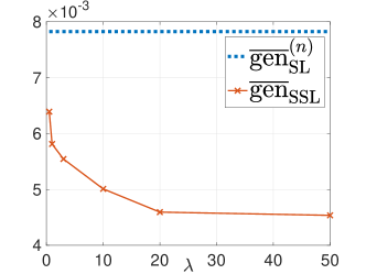
Figure 4: Empirical gen-error of logistic regression on MNIST dataset.

Recall the proof of Corollary 1 in Appendix J. In the logistic regression with $l_{2}$ regularization, the unique minimizer of the empirical risk in (15) is rewritten as

$$\hat{\mathbf{W}}_{\mathrm{ML}}(S_{\mathrm{l}},\hat{S}_{\mathrm{u}})=\operatorname*{arg\,min}_{\mathbf{w}\in\mathcal{W}}\bigg{(}-\frac{1}{1+\lambda}\frac{1}{n}\sum_{i=1}^{n}\log p(\mathbf{Z}_{i}|\mathbf{w})-\frac{\lambda}{1+\lambda}\frac{1}{m}\sum_{i=n+1}^{n+m}\log p(\hat{\mathbf{Z}}_{i}|\mathbf{w})+\frac{\nu}{2}\|\mathbf{w}\|_{2}^{2}\bigg{)}$$ (167)

and the Hessian matrix of the empirical risk at $\mathbf{w}=\hat{\mathbf{W}}_{\mathrm{ML}}(S_{\mathrm{l}},\hat{S}_{\mathrm{u}})$ is rewritten as

$$H^{*}(S_{\mathrm{l}},\hat{S}_{\mathrm{u}})=\nabla_{\mathbf{w}}^{2}\bigg{(}-\frac{1}{1+\lambda}\frac{1}{n}\sum_{i=1}^{n}\log p(\mathbf{Z}_{i}|\mathbf{w})-\frac{\lambda}{1+\lambda}\frac{1}{m}\sum_{i=n+1}^{n+m}\log p(\hat{\mathbf{Z}}_{i}|\mathbf{w})\bigg{)}\bigg{|}_{\mathbf{w}=\hat{\mathbf{W}}_{\mathrm{ML}}(S_{\mathrm{l}},\hat{S}_{\mathrm{u}})}+\nu\mathbf{I}_{d}.$$ (168)

Recall the definition of $\mathbf{w}^{*}_{\lambda}$ with regularization

$$\mathbf{w}^{*}_{\lambda}= \operatorname*{arg\,min}_{\mathbf{w}\in\mathcal{W}}\bigg{(}\frac{n}{n+m}D\big{(}P_{\mathbf{Z}}\|p(\cdot|\mathbf{w})\big{)}+\frac{m}{n+m}D\big{(}P_{\hat{\mathbf{Z}}|\mathbf{w}^{*}_{0}}\|p(\cdot|\mathbf{w})\big{)}+\frac{\nu}{2}\|\mathbf{w}\|_{2}^{2}\bigg{)}.$$ (169)

Given any ratio $\lambda>0$, as $n,m\to\infty$, the Hessian matrix converges as follows

$$H^{*}(S_{\mathrm{l}},\hat{S}_{\mathrm{u}})\xrightarrow{\mathrm{p}}J(\mathbf{w}^{*}_{\lambda})+\nu\mathbf{I}_{d}.$$ (170)

Then the asymptotic expected gen-error in (145) is rewritten as

$$\overline{\mathrm{gen}}(P_{\mathbf{W}|S_{\mathrm{l}},\hat{S}_{\mathrm{u}}}^{\infty},P_{S_{\mathrm{l}},\hat{S}_{\mathrm{u}}})$$

$$=\frac{n+m}{n}\operatorname{tr}\bigg{(}\!\mathbb{E}_{\hat{S}_{\mathrm{u}}}\mathbb{E}_{S_{\mathrm{l}}}\!\bigg{[}\big{(}\hat{\mathbf{W}}_{\mathrm{ML}}(S_{\mathrm{l}},\hat{S}_{\mathrm{u}})-\mathbb{E}_{S_{\mathrm{l}}}[\hat{\mathbf{W}}_{\mathrm{ML}}(S_{\mathrm{l}},\hat{S}_{\mathrm{u}})]\big{)}\big{(}\hat{\mathbf{W}}_{\mathrm{ML}}(S_{\mathrm{l}},\hat{S}_{\mathrm{u}})-\mathbb{E}_{S_{\mathrm{l}}}[\hat{\mathbf{W}}_{\mathrm{ML}}(S_{\mathrm{l}},\hat{S}_{\mathrm{u}})]\big{)}^{\top}\!\bigg{]}(J(\mathbf{w}^{*}_{\lambda})+\nu\mathbf{I}_{d})\!\bigg{)}.$$ (171)

By redefining $\hat{\mathbf{W}}(\hat{s}_{\mathrm{u}})$ in (146) with the $l_{2}$ regularization term $\frac{\nu}{2}\|\mathbf{w}\|_{2}^{2}$, we can similarly obtain

$$\hat{\mathbf{W}}_{\mathrm{ML}}(S_{\mathrm{l}},\hat{S}_{\mathrm{u}}) \xrightarrow{\mathrm{d}}\mathcal{N}\bigg{(}\mathbf{w}^{*}_{\lambda},\frac{n(J(\mathbf{w}^{*}_{\lambda})+\nu\mathbf{I}_{d})^{-1}\mathcal{I}_{\mathrm{l}}(\mathbf{w}^{*}_{\lambda})(J(\mathbf{w}^{*}_{\lambda})+\nu\mathbf{I}_{d})^{-1}}{(n+m)^{2}}\bigg{)}.$$ (172)

Then the expected gen-error in (145) can be rewritten as

$$\overline{\mathrm{gen}}(P_{\mathbf{W}|S_{\mathrm{l}},\hat{S}_{\mathrm{u}}}^{\infty},P_{S_{\mathrm{l}},\hat{S}_{\mathrm{u}}}) =\frac{\operatorname{tr}((J(\mathbf{w}^{*}_{\lambda})+\nu\mathbf{I}_{d})^{-1}\mathcal{I}_{\mathrm{l}}(\mathbf{w}^{*}_{\lambda}))}{n+m}.$$ (173)

Similarly, the excess risk in (19) can be rewritten as

$$\mathcal{E}_{\mathrm{r}}(P_{\mathbf{W}})=\frac{1}{2}\operatorname{tr}((\mathbf{w}^{*}_{\lambda}-\mathbf{w}^{*}_{\mathrm{l}})(\mathbf{w}^{*}_{\lambda}-\mathbf{w}^{*}_{\mathrm{l}})^{\top}J_{\mathrm{l}}(\mathbf{w}_{\mathrm{l}}^{*}))+\frac{\operatorname{tr}(J_{\mathrm{l}}(\mathbf{w}_{\mathrm{l}}^{*})(J(\mathbf{w}^{*}_{\lambda})+\nu\mathbf{I}_{d})^{-1}\mathcal{I}_{\mathrm{l}}(\mathbf{w}^{*}_{\lambda})(J(\mathbf{w}^{*}_{\lambda})+\nu\mathbf{I}_{d})^{-1})}{2(1+\lambda)(n+m)},$$ (174)

where $\mathbf{w}_{\mathrm{l}}^{*}=\operatorname*{arg\,min}_{\mathbf{w}\in\mathcal{W}}L_{\mathrm{P}}(\mathbf{W},P_{S_{\mathrm{l}}})$.

In addition to the experiments on the synthetic datasets, we implement an logistic regression experiment on “0–1” digit pair in MNIST dataset by setting $n=200$, $\lambda\in\{0.5,1,3,10,20,50\}$ and $\nu=5$. In Figure 4, we observe that the gen-error decreases as $\lambda$ increases.

References

- Amini and Gallinari (2002) Massih-Reza Amini and Patrick Gallinari. Semi-supervised logistic regression. In ECAI, volume 2, page 11, 2002.
- Aminian et al. (2015) Gholamali Aminian, Hamidreza Arjmandi, Amin Gohari, Masoumeh Nasiri-Kenari, and Urbashi Mitra. Capacity of diffusion-based molecular communication networks over LTI-Poisson channels. IEEE Transactions on Molecular, Biological and Multi-Scale Communications, 1(2):188–201, 2015.
- Aminian et al. (2021a) Gholamali Aminian, Yuheng Bu, Laura Toni, Miguel Rodrigues, and Gregory Wornell. An exact characterization of the generalization error for the Gibbs algorithm. Advances in Neural Information Processing Systems, 34, 2021a.
- Aminian et al. (2021b) Gholamali Aminian, Laura Toni, and Miguel RD Rodrigues. Information-theoretic bounds on the moments of the generalization error of learning algorithms. In IEEE International Symposium on Information Theory (ISIT), 2021b.
- Aminian et al. (2022a) Gholamali Aminian, Mahed Abroshan, Mohammad Mahdi Khalili, Laura Toni, and Miguel Rodrigues. An information-theoretical approach to semi-supervised learning under covariate-shift. In International Conference on Artificial Intelligence and Statistics, pages 7433–7449. PMLR, 2022a.
- Aminian et al. (2022b) Gholamali Aminian, Saeed Masiha, Laura Toni, and Miguel RD Rodrigues. Learning algorithm generalization error bounds via auxiliary distributions. arXiv preprint arXiv:2210.00483, 2022b.
- Arazo et al. (2020) Eric Arazo, Diego Ortego, Paul Albert, Noel E O’Connor, and Kevin McGuinness. Pseudo-labeling and confirmation bias in deep semi-supervised learning. In 2020 International Joint Conference on Neural Networks (IJCNN), pages 1–8. IEEE, 2020.
- Asadi et al. (2018) Amir Asadi, Emmanuel Abbe, and Sergio Verdú. Chaining mutual information and tightening generalization bounds. In Advances in Neural Information Processing Systems, pages 7234–7243, 2018.
- Asadi and Abbe (2020) Amir R Asadi and Emmanuel Abbe. Chaining meets chain rule: Multilevel entropic regularization and training of neural networks. Journal of Machine Learning Research, 21(139):1–32, 2020.
- Athreya and Hwang (2010) KB Athreya and Chii-Ruey Hwang. Gibbs measures asymptotics. Sankhya A, 72(1):191–207, 2010.
- Berthelot et al. (2019) David Berthelot, Nicholas Carlini, Ian Goodfellow, Nicolas Papernot, Avital Oliver, and Colin A Raffel. Mixmatch: A holistic approach to semi-supervised learning. Advances in neural information processing systems, 32, 2019.
- Bu et al. (2020) Yuheng Bu, Shaofeng Zou, and Venugopal V Veeravalli. Tightening mutual information-based bounds on generalization error. IEEE Journal on Selected Areas in Information Theory, 1(1):121–130, 2020.
- Bu et al. (2022) Yuheng Bu, Gholamali Aminian, Laura Toni, Gregory W Wornell, and Miguel Rodrigues. Characterizing and understanding the generalization error of transfer learning with gibbs algorithm. In International Conference on Artificial Intelligence and Statistics, pages 8673–8699. PMLR, 2022.
- Castelli and Cover (1996) Vittorio Castelli and Thomas M Cover. The relative value of labeled and unlabeled samples in pattern recognition with an unknown mixing parameter. IEEE Transactions on Information Theory, 42(6):2102–2117, 1996.
- Catoni (2007) Olivier Catoni. PAC-Bayesian supervised classification: the thermodynamics of statistical learning. arXiv preprint arXiv:0712.0248, 2007.
- Chapelle et al. (2003) Olivier Chapelle, Jason Weston, and Bernhard Scholkopf. Cluster kernels for semi-supervised learning. Advances in neural information processing systems, pages 601–608, 2003.
- Chapelle et al. (2006) Olivier Chapelle, Bernhard Schölkopf, and Alexander Zien, editors. Semi-Supervised Learning. The MIT Press, 2006.
- Chiang et al. (1987) Tzuu-Shuh Chiang, Chii-Ruey Hwang, and Shuenn Jyi Sheu. Diffusion for global optimization in . SIAM Journal on Control and Optimization, 25(3):737–753, 1987.
- Cover (1999) Thomas M Cover. Elements of information theory. John Wiley & Sons, 1999.
- Dupre et al. (2019) Robert Dupre, Jiri Fajtl, Vasileios Argyriou, and Paolo Remagnino. Improving dataset volumes and model accuracy with semi-supervised iterative self-learning. IEEE Transactions on Image Processing, 29:4337–4348, 2019.
- Esposito et al. (2021) Amedeo Roberto Esposito, Michael Gastpar, and Ibrahim Issa. Generalization error bounds via Rényi-, f-divergences and maximal leakage. IEEE Transactions on Information Theory, 2021.
- Gibbs (1902) Josiah Willard Gibbs. Elementary principles of statistical mechanics. Compare, 289:314, 1902.
- Göpfert et al. (2019) Christina Göpfert, Shai Ben-David, Olivier Bousquet, Sylvain Gelly, Ilya Tolstikhin, and Ruth Urner. When can unlabeled data improve the learning rate? In Conference on Learning Theory, pages 1500–1518. PMLR, 2019.
- Grandvalet et al. (2005) Yves Grandvalet, Yoshua Bengio, et al. Semi-supervised learning by entropy minimization. CAP, 367:281–296, 2005.
- Hafez-Kolahi et al. (2020) Hassan Hafez-Kolahi, Zeinab Golgooni, Shohreh Kasaei, and Mahdieh Soleymani. Conditioning and processing: Techniques to improve information-theoretic generalization bounds. Advances in Neural Information Processing Systems, 33, 2020.
- Haghifam et al. (2020) Mahdi Haghifam, Jeffrey Negrea, Ashish Khisti, Daniel M Roy, and Gintare Karolina Dziugaite. Sharpened generalization bounds based on conditional mutual information and an application to noisy, iterative algorithms. Advances in Neural Information Processing Systems, 2020.
- He et al. (2022) Haiyun He, Hanshu Yan, and Vincent YF Tan. Information-theoretic characterization of the generalization error for iterative semi-supervised learning. Journal of Machine Learning Research, 23:1–52, 2022.
- Iscen et al. (2019) Ahmet Iscen, Giorgos Tolias, Yannis Avrithis, and Ondrej Chum. Label propagation for deep semi-supervised learning. In Proceedings of the IEEE/CVF Conference on Computer Vision and Pattern Recognition, pages 5070–5079, 2019.
- Jaynes (1957) Edwin T Jaynes. Information theory and statistical mechanics. Physical review, 106(4):620, 1957.
- Jeffreys (1946) Harold Jeffreys. An invariant form for the prior probability in estimation problems. Proceedings of the Royal Society of London. Series A. Mathematical and Physical Sciences, 186(1007):453–461, 1946.
- Ji et al. (2012) Ming Ji, Tianbao Yang, Binbin Lin, Rong Jin, and Jiawei Han. A simple algorithm for semi-supervised learning with improved generalization error bound. In Proceedings of the 29th International Coference on International Conference on Machine Learning, pages 835–842, 2012.
- Kuzborskij et al. (2019) Ilja Kuzborskij, Nicolò Cesa-Bianchi, and Csaba Szepesvári. Distribution-dependent analysis of Gibbs-ERM principle. In Conference on Learning Theory, pages 2028–2054. PMLR, 2019.
- Lee et al. (2013) Dong-Hyun Lee et al. Pseudo-label: The simple and efficient semi-supervised learning method for deep neural networks. In Workshop on Challenges in Representation Learning, ICML, 2013.
- Li et al. (2019) Jian Li, Yong Liu, Rong Yin, and Weiping Wang. Multi-class learning using unlabeled samples: Theory and algorithm. In International Joint Conference on Artificial Intelligence (IJCAI), pages 2880–2886, 2019.
- Markowich and Villani (2000) Peter A Markowich and Cédric Villani. On the trend to equilibrium for the Fokker-Planck equation: an interplay between physics and functional analysis. Mat. Contemp, 19:1–29, 2000.
- McLachlan (2005) Geoffrey J McLachlan. Discriminant Analysis and Statistical Pattern Recognition. John Wiley & Sons, 2005.
- Moon (1996) Todd K Moon. The expectation-maximization algorithm. IEEE Signal processing magazine, 13(6):47–60, 1996.
- Niu et al. (2013) Gang Niu, Wittawat Jitkrittum, Bo Dai, Hirotaka Hachiya, and Masashi Sugiyama. Squared-loss mutual information regularization: A novel information-theoretic approach to semi-supervised learning. In International Conference on Machine Learning, pages 10–18. PMLR, 2013.
- Ouali et al. (2020) Yassine Ouali, Céline Hudelot, and Myriam Tami. An overview of deep semi-supervised learning. arXiv preprint arXiv:2006.05278, 2020.
- Palomar and Verdú (2008) Daniel P Palomar and Sergio Verdú. Lautum information. IEEE transactions on information theory, 54(3):964–975, 2008.
- Raginsky et al. (2017) Maxim Raginsky, Alexander Rakhlin, and Matus Telgarsky. Non-convex learning via stochastic gradient Langevin dynamics: a nonasymptotic analysis. In Conference on Learning Theory, pages 1674–1703. PMLR, 2017.
- Rigollet (2007) Philippe Rigollet. Generalization error bounds in semi-supervised classification under the cluster assumption. Journal of Machine Learning Research, 8(7), 2007.
- Rizve et al. (2020) Mamshad Nayeem Rizve, Kevin Duarte, Yogesh S Rawat, and Mubarak Shah. In defense of pseudo-labeling: An uncertainty-aware pseudo-label selection framework for semi-supervised learning. In International Conference on Learning Representations, 2020.
- Russo and Zou (2019) Daniel Russo and James Zou. How much does your data exploration overfit? controlling bias via information usage. IEEE Transactions on Information Theory, 66(1):302–323, 2019.
- Seeger (2000) Matthias Seeger. Learning with labeled and unlabeled data. 2000. URL http://infoscience.epfl.ch/record/161327.
- Singh et al. (2008) Aarti Singh, Robert Nowak, and Jerry Zhu. Unlabeled data: Now it helps, now it doesn’t. Advances in Neural Information Processing Systems, 21:1513–1520, 2008.
- Sohn et al. (2020) Kihyuk Sohn, David Berthelot, Nicholas Carlini, Zizhao Zhang, Han Zhang, Colin A Raffel, Ekin Dogus Cubuk, Alexey Kurakin, and Chun-Liang Li. Fixmatch: Simplifying semi-supervised learning with consistency and confidence. Advances in neural information processing systems, 33:596–608, 2020.
- Steinke and Zakynthinou (2020) Thomas Steinke and Lydia Zakynthinou. Reasoning about generalization via conditional mutual information. In Conference on Learning Theory, pages 3437–3452. PMLR, 2020.
- Szummer and Jaakkola (2002) Martin Szummer and Tommi Jaakkola. Information regularization with partially labeled data. Advances in Neural Information processing systems, 15, 2002.
- Vershynin (2018) Roman Vershynin. High-dimensional probability: An introduction with applications in data science, volume 47. Cambridge university press, 2018.
- Wei et al. (2020) Colin Wei, Kendrick Shen, Yining Chen, and Tengyu Ma. Theoretical analysis of self-training with deep networks on unlabeled data. In International Conference on Learning Representations, 2020.
- Xu and Raginsky (2017) Aolin Xu and Maxim Raginsky. Information-theoretic analysis of generalization capability of learning algorithms. In Advances in Neural Information Processing Systems, pages 2524–2533, 2017.
- Zhu (2020) Jingge Zhu. Semi-supervised learning: the case when unlabeled data is equally useful. In Conference on Uncertainty in Artificial Intelligence, pages 709–718. PMLR, 2020.
- Zhu and Goldberg (2009) Xiaojin Zhu and Andrew B Goldberg. Introduction to semi-supervised learning. Synthesis Lectures on Artificial Intelligence and Machine Learning, 3(1):1–130, 2009.
- Zhu (2008) Xiaojin Jerry Zhu. Semi-supervised learning literature survey. Technical report, University of Wisconsin-Madison Department of Computer Sciences, 2008.