Panchromatic and Multispectral Image Fusion via Alternating Reverse Filtering Network

Abstract

Panchromatic (PAN) and multi-spectral (MS) image fusion, named Pan-sharpening, refers to super-resolve the low-resolution (LR) multi-spectral (MS) images in the spatial domain to generate the expected high-resolution (HR) MS images, conditioning on the corresponding high-resolution PAN images. In this paper, we present a simple yet effective alternating reverse filtering network for pan-sharpening. Inspired by the classical reverse filtering that reverses images to the status before filtering, we formulate pan-sharpening as an alternately iterative reverse filtering process, which fuses LR MS and HR MS in an interpretable manner. Different from existing model-driven methods that require well-designed priors and degradation assumptions, the reverse filtering process avoids the dependency on pre-defined exact priors. To guarantee the stability and convergence of the iterative process via contraction mapping on a metric space, we develop the learnable multi-scale Gaussian kernel module, instead of using specific filters. We demonstrate the theoretical feasibility of such formulations. Extensive experiments on diverse scenes to thoroughly verify the performance of our method, significantly outperforming the state of the arts.

1 Introduction

Multispectral images are widely used in various fields such as resource monitoring [1], environmental protection [2, 3] and ecological monitoring [4]. However, due to the hardware limitations of multispectral sensors, multispectral images usually lack high spatial resolution [5, 6]. In contrast, high-resolution panchromatic (PAN) images that contain rich spatial details of the same scene are easy to obtain. Therefore, pan-sharpening, generating high-resolution multispectral images by fusing panchromatic images with low-resolution multispectral images, has become an important issue in the field of remote sensing [7, 8].

Many efforts have been made to solve the pan-sharpening problem, which can be generally divided into two large groups: traditional pan-sharpening methods and deep learning-based methods [9, 10]. Traditional pan-sharpening methods usually require strict assumptions of multispectral image degradation via prior knowledge. Otherwise, the inexact assumptions may cause system model error. For example, both the assumptions established by component substitution methods [11, 12] and multi-resolution analysis methods [13, 14] focus on the relationship between PAN and HR MS, which is destined to make these methods prone to spectral distortion. Unlike the above-mentioned traditional approaches, variational optimization approaches consider the relationship among HR MS, LR MS and PAN, and then construct the energy function based on well-designed priors [15, 16]. However, the methods of this kind inflict high computational burden, restricting their practical applications.

Most recently, deep learning exhibited outstanding performance in the field of remote sensing images [17, 18]. Undoubtedly, the deep learning-based (DL) methods become a newly developed category to solve pan-sharpening [19, 20, 21, 22]. Unfortunately, the pan-sharpening networks commonly lack the interpretability in theirs designs, which limits their performance. To solve this issue, the model-based deep learning methods build the network by unrolling the specific optimization algorithm [23, 24]. However, the optimization algorithms of model-based deep learning methods still require well-designed priors or assumptions. Additionally, the convergence of the optimization algorithms is not taken into account in the design of the unrolling networks.

To address these problems, we propose a novel pan-sharpening approach called alternating reverse filtering network, which combines classical reverse filtering [25] and deep learning. Unlike previous methods, we formulate pan-sharpening as a reverse filtering process, thus avoiding the dependency on pre-defined priors or assumption. In addition, we tailor the classical reverse filtering in an alternating iteration manner for the pan-sharpening problem. The process of alternating iterations is unrolled into a network. We demonstrate such formulations is theoretical feasibility. To guarantee the stability and convergence of the iterative process on the basis of contraction mapping in a metric space, we introduce the learnable multi-scale Gaussian kernel module in the network. Such a key issue is commonly neglected in previous unrolling-based deep learning methods.

The main contributions of this paper can be summarized as follows: 1) We introduce a new perspective for pan-sharpening by formulating it as a reverse filtering process. To the best of our knowledge, this is the first effort to solve multispectral image fusion problem using the method of this kind. 2) In contrast to existing model-driven methods, our iterative network can obtain HR MS without the need for pre-defined exact priors or assumptions. 3) Instead of using specific filters in reverse filtering, we constrain their formulation in a more compact learnable multi-scale Gaussian kernel module, which guarantees the stability and convergence of the iterative process. In addition, extensive experimental results on simulated and real-world scenes show that the proposed network significantly outperforms the state of the arts.

2 Related Work

Pan-sharpening. Traditional pan-sharpening methods are classified into three types: component substitution (CS)-, multi-resolution analysis (MRA)-, and variational optimization (VO)-based methods [26, 16, 27, 28, 29]. The main idea of CS-based methods is to separate spatial and spectral information of the MS image in a suitable space and further fuse them with the PAN image. The representative CS-based methods include intensity hue-saturation (IHS) fusion [30], the principal component analysis (PCA) methods [11, 31], Brovey transforms [32], and Gram-Schmidt (GS) orthogonalization method [33]. MRA-based methods decompose MS and PAN images into multi-scale space via decimated wavelet transform (DWT) [34], high-pass filter fusion (HPF) [35], indusion method [13] and atrous wavelet transform (ATWT) [36]. Then, the decomposed version PAN images are injected into the corresponding MS images for information fusion. VO-based methods regard the pan-sharpening tasks as an ill-posed problem by minimizing a loss function, including dynamic gradient sparsity property (SIRF) [37], local gradient constraint (LGC) [15], group low-rank constraint for texture similarity (ADMM) [16]. However, the performance of these methods is limited due to the shallow non-linear expression in these models. Since then, deep learning-based pan-sharpening algorithms have dominated this field [9, 38, 39]. Masi et al. [9] are the first to use CNN to deal with the issue of pan-sharpening. Although the structure is simple, the effect is much better than the traditional methods. Then, Yang et al. [38] designed a deeper CNN by relying on resblock in [40]. Meanwhile, Yuan et al. [41] introduced multi-scale module into the basic CNN architecture.

Unrolling-based deep learning method. In recent years, many researchers [42, 43, 44, 45, 46, 47] attempt to combine domain knowledge with deep neural networks to propose deep unrolling networks which take advantages of the model-based methods’ interpretability and learning-based methods’ strong mapping ability. Specifically, the deep unrolling network firstly unrolls certain optimization algorithms [48, 49, 50, 23, 51, 52, 53, 54, 55, 56, 57] and utilizes deep neural network to parameterize the unrolling model, then minimizes the loss function and optimizes the parameters in an end-to-end manner. For example, Xu et al. [24] developed two separate priors of PAN and MS modality to design the unrolling structure for pan-sharpening. The model-driven methods have better interpretability and clearer physical meaning. Cao et al. [46] unrolled an alternate optimization algorithm into CNN. However, the optimization of model-based deep methods also require well-designed priors and exact degradation assumptions.

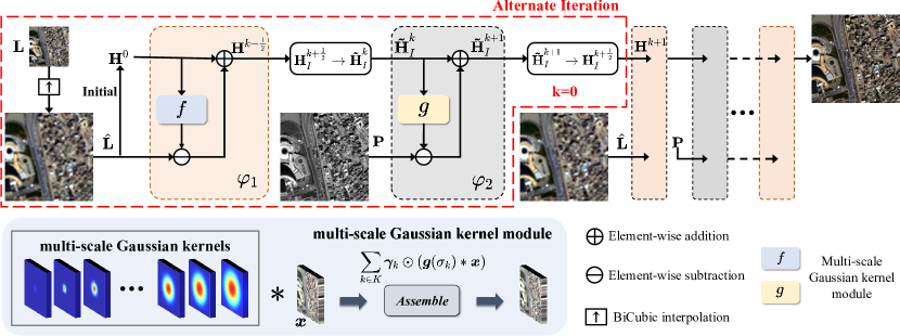
Figure 1: The overall architecture of alternating reverse filtering network.

3 Proposed Method

In this section, we provide a detailed introduction to our proposed alternating reverse filtering network for pan-sharpening. For convenience, we first define some notations. Concretely, $\mathbf{L}\in\mathbb{R}^{w\times h\times B}$ denotes the low-resolution (LR) multispectral image, $\mathbf{H}\in\mathbb{R}^{W\times H\times B}$ represents the corresponding high-resolution (HR) multispectral image, and $\mathbf{P}\in\mathbb{R}^{W\times H\times b}$ is the PAN image.

3.1 Problem Formulation

For multispectral image restoration, the degradation model is commonly formulated as

$$\mathbf{L}=(\mathbf{H}\ast\mathbf{k})\downarrow_{\mathbf{s}}+\bm{\epsilon},$$ (1)

where $\ast$, $\mathbf{k}$, ${\downarrow_{\mathbf{s}}}$ and $\bm{\epsilon}$ denote the convolution operation, blurring kernel, down-sampling operator and the measurement noise, respectively. To restore high quality $\mathbf{H}$ from $\mathbf{L}$, high-resolution PAN image $\mathbf{P}$ is introduced to help enhance structural detail. In CS-based models, the intensity component $\mathbf{I}$, a generalized IHS concept [58], is usually replaced by $\mathbf{P}$ but the discrepancy between $\mathbf{P}$ and $\mathbf{I}$ can cause spectral distortion in the fused image. The VO-based models solve the problem by explicitly constructing many well-designed priors among $\mathbf{H}$, $\mathbf{L}$ and $\mathbf{P}$. However, hand-crafted priors don’t work well in practical complex situations. Inspired by classical reverse filtering [25], we propose alternating reverse filtering method to estimate $\mathbf{H}$ by the more general multispectral image priors:

$$\mathbf{L} = f(\mathbf{H}),$$ (2)

$$\mathbf{P} = g(\mathbf{H}_{I}),$$ (3)

where $f(\cdot)$ and $g(\cdot)$ denote the degradation processes, and $\mathbf{H}_{I}$ is the intensity component of $\mathbf{H}$.

3.2 Model Optimization

Definition 3.2

Suppose $(\mathcal{H},d)$ is a metric space and $T:\mathcal{H}\rightarrow\mathcal{H}$ is a mapping function. For all $x,y\in\mathcal{H}$, if there exists a constant $c\in[0,1)$ that makes the following formula

$$d(T(x),T(y))\leq cd(x,y),$$ (4)

mapping $T:\mathcal{H}\rightarrow\mathcal{H}$ is called Contraction Mapping[59].

In the image space, the metric space $(\mathcal{H},d)$ can be expressed as

$$\mathcal{H}=R^{w\times h},\\ d(x,y)=\|x-y\|,$$ (5)

where $w\times h$ is the number of image pixels and $d(x,y)$ is the Euclidean distance.

Theorem 3.2

A variable $x^{*}$ is a fixed point for a given function $\Phi$ if $\Phi(x^{*})=x^{*}$. When mapping $\Phi:\mathcal{H}\rightarrow\mathcal{H}$ is a contraction mapping, $\Phi$ admits a unique fixed-point $x^{*}$ in $\mathcal{H}$. Further, $x^{*}$ can be found in the following way. Let the initial guess be $x_{0}$ and define a sequence $\left\{x_{n}\right\}$ as $x_{n}=\Phi(x_{n-1})$. When the iterative process converges, $\lim_{n\rightarrow\infty}x_{n}=x^{*}$.

Reverse Filtering

Without loss of generality, the degenerate processes $f(\cdot)$ and $g(\cdot)$ can be considered as broadly defined filters $F(\cdot)$ that smooth images, texture removal or other properties. Filtering process can be described as

$$\bm{y}=F(\bm{x}),$$ (6)

where $\bm{x}$ and $\bm{y}$ are the input image and the filtering result. When $F(\cdot)$ is unknown, it’s difficult to apply well-designed image priors to obtain the $\bm{x}$. However, reverse filtering can estimate $\bm{x}$ without needing to compute $F^{-1}(\cdot)$ and update restored images according to the filtering effect as

$$\bm{x}^{k+1}=\bm{x}^{k}+\bm{y}-F(\bm{x}^{k}),$$ (7)

where $\bm{x}^{k}$ is the current estimate of $\bm{x}$ in the k-th iteration. The iteration starts from $\bm{x}^{0}=\bm{y}$ and $\bm{x}^{k}$ gets closer and closer to $\bm{x}$ with the increasing ${k}$. We make auxiliary function $\varphi(\cdot)$ as

$$\varphi(\bm{x})=\bm{x}+\bm{y}-F(\bm{x}).$$ (8)

Therefore, the above iterative process can be regarded as a fixed point iteration

$$\bm{x}^{k+1}=\varphi(\bm{x}^{k}).$$ (9)

With the above analysis, we take the filtering function $F(\cdot)$ in Equation 8 as $f(\cdot)$ and $g(\cdot)$ in Equation 2 to obtain two reverse filtering:

$$\left\{\begin{array}[]{lcl}\varphi_{1}(\mathbf{H})&=&\mathbf{H}+\mathbf{\hat{L}}-f(\mathbf{H})\\ \varphi_{2}(\mathbf{H}_{I})&=&\mathbf{H}_{I}+\mathbf{P}-g(\mathbf{H}_{I}),\end{array}\right.$$ (12)

and hence our alternating reverse filtering method can be written by following

$$\left\{\begin{array}[]{lcl}\mathbf{H}^{k+\frac{1}{2}}&=&\mathbf{H}^{k}+\mathbf{\hat{L}}-f(\mathbf{H}^{k})\\ \mathbf{\tilde{H}}_{I}^{k}&=&\mathbf{H}_{I}^{k+\frac{1}{2}}\\ \mathbf{\tilde{H}}_{I}^{k+1}&=&\mathbf{\tilde{H}}_{I}^{k}+\mathbf{P}-g(\mathbf{\tilde{H}}_{I}^{k})\\ \mathbf{H}^{k+1}&\Leftarrow&(\mathbf{H}_{I}^{k+\frac{1}{2}}\leftarrow\mathbf{\tilde{H}}_{I}^{k+1}),\end{array}\right.$$ (17)

where $\mathbf{\hat{L}}$ is the upsampled LR multispectral image $\mathbf{L}$ and $\mathbf{\tilde{H}}_{I}^{k}$ is an approximate estimate of $\mathbf{H}_{I}$. Equation 17 starts with initial state $\mathbf{H}^{0}=\mathbf{\hat{L}}$. Note that the calculated $\mathbf{H}^{k+\frac{1}{2}}$ is used as input in the next iteration, the intensity component $\mathbf{H}_{I}^{k+\frac{1}{2}}$ is then sent into another iteration $\mathbf{\tilde{H}}_{I}^{k+1}=\mathbf{\tilde{H}}_{I}^{k}+\mathbf{P}-g(\mathbf{\tilde{H}}_{I}^{k})$ to enhance the structural details with the help of $\mathbf{P}$ image. After that, the enhanced intensity component replaces the original component $\mathbf{H}_{I}^{k+\frac{1}{2}}\leftarrow\mathbf{\tilde{H}}_{I}^{k+1}$ and the new $\mathbf{H}^{k+1}$ is used as input in the next iteration.

3.3 Alternating Reverse Filtering Network

The end-to-end model we construct for GMIR, named as ARFNet (Alternating Reverse Filtering Network), is based on two fixed point iterations in Equation 17 with multi-scale Gaussian convolution module acting as filters. See Figure 1 for the overview of the proposed method. If reverse filtering satisfies the sufficient condition for definition  3.2, ARFNet will converge $\lim_{k\rightarrow\infty}\mathbf{H}^{k}=\mathbf{H}^{*}$ and finally reaches $f\left(\mathbf{H}^{*}\right)\approx\mathbf{\hat{L}}$. Take the $\varphi_{1}(\cdot)$ for instance, the sufficient condition that theorem  3.2 holds is that $\varphi_{1}(\mathbf{H})$ forms a contraction mapping

$$\begin{aligned} \left\|\varphi_{1}\left(\mathbf{H}_{a}\right)-\varphi_{1}\left(\mathbf{H}_{b}\right)\right\|&=\left\|\left[\mathbf{H}_{a}+\mathbf{\hat{L}}-f\left(\mathbf{H}_{a}\right)\right]-\left[\mathbf{H}_{b}+\mathbf{\hat{L}}-f\left(\mathbf{H}_{b}\right)\right]\right\|\\ &=\left\|\left[\mathbf{H}_{a}-f\left(\mathbf{H}_{a}\right)\right]-\left[\mathbf{H}_{b}-f\left(\mathbf{H}_{b}\right)\right]\right\|\leq c\cdot\left\|\mathbf{H}_{a}-\mathbf{H}_{b}\right\|,\quad c\in[0,1)\end{aligned}$$ (18)

For linear filters, the condition is further simplified as

$$\|\mathbf{H}-f(\mathbf{H})\|\leq c\cdot\|\mathbf{H}\|.\quad c\in[0,1)$$ (19)

In our case, the degenerate processes $f(\cdot)$ and $g(\cdot)$ are implemented by multi-scale Gaussian convolution modules.

Multi-scale Gaussian Convolution Module

Given an input image $\bm{x}$, the output $\bm{y}$ of Gaussian convolution [60] can be expressed as

$$\bm{y}=\bm{g}(\sigma_{k})*\bm{x},$$ (20)

where $\sigma_{k}$ denotes the variance of 2D Gaussian kernels. In particular, we define $\sigma_{1}=0$ and $\bm{g}(\sigma_{1})={\bm{\delta}}$ which is Dirac delta. Therefore,

$$\|\mathbf{H}*(\bm{g}(\sigma_{1})-\bm{g}(\sigma))\|=\|\widehat{\mathbf{H}}\odot(\mathbf{1}-\bm{\widehat{g}(\sigma)})\|\leq c\cdot\|\widehat{\mathbf{H}}\|=c\cdot\|\mathbf{H}\|,$$ (21)

where $\widehat{\bm{H}}$ denotes Fourier transform, $\odot$ denotes point-wised product and $\bm{1}$ denotes all-one matrix. Thus, the inequality holds true when $\bm{g}(\sigma_{k})$ is a normalized Gaussian kernel that means these filters can be strictly reversed using fixed-point iteration. In our model, normalized Gaussian kernel is used for initialization and its parameters can be further learned from the data in an end-to-end manner. Although the learned convolution kernels may not completely satisfy the condition, fixed point iteration can be split into two independent sequences:

$$\mathbf{H}^{k+1}=\mathbf{H}_{c}^{k+1}+\mathbf{H}_{o}^{k+1}=\varphi_{1}\left(\mathbf{H}_{c}^{k}\right)+\varphi_{1}\left(\mathbf{H}_{o}^{k}\right),$$ (22)

where $\{\mathbf{H}_{c}^{k}\}$ is guaranteed to converge to the unique solution and $\{\mathbf{H}_{o}^{k}\}$ could oscillate. Fortunately, after the first few epochs, the learned convolution kernels are close to the kernels we initialize, which makes $\{\mathbf{H}_{c}^{k}\}$ the majority and dominates the convergence of the whole process. In the implementation of the algorithm, we adopt multi-scale Gaussian convolution module to obtain better filtering effect. Compared to Gaussian convolution, the multi-scale Gaussian convolution module integrates Gaussian kernels with different kernel sizes, expressed as

$$\bm{y}=\sum_{k\in K}\bm{\gamma}_{k}\odot(\bm{g}(\sigma_{k})*\bm{x}),K=\{1,3,5,\cdot\cdot\cdot,M\},$$ (23)

where $\gamma_{k}$ is the learnable mixing coefficient and $k$ denotes different kernel sizes $1\times 1,3\times 3,5\times 5,\cdot\cdot\cdot,M\times M$. The multi-scale Gaussian convolution is a series simple group convolutional layers defined by initialized 2D Gaussian kernels. Clearly, the form of weighted summation still conforms to the above analysis about sufficient condition.

Taken together, the forward process of alternating reverse filtering network can be described as Algorithm  1.

Algorithm 1 Proposed algorithm.

The upsampled low-resolution multispectral image $\mathbf{\hat{L}}$, panchromatic image $\mathbf{P}$ and maximum iteration number $K$.

initial $\mathbf{H}^{0}=\mathbf{\hat{L}}$;

for $k=0,1,2,3,\cdot\cdot\cdot,K$ do

     compute $\mathbf{H}^{k+\frac{1}{2}}=\mathbf{H}^{k}+\mathbf{\hat{L}}-f(\mathbf{H}^{k})$;

     fetch the intensity component $\mathbf{\tilde{H}}_{I}^{k}=\mathbf{H}_{I}^{k+\frac{1}{2}}$;

     compute $\mathbf{\tilde{H}}_{I}^{k+1}=\mathbf{\tilde{H}}_{I}^{k}+\mathbf{P}-g(\mathbf{\tilde{H}}_{I}^{k})$;

     replace the intensity component $\mathbf{H}_{I}^{k+\frac{1}{2}}\leftarrow\mathbf{\tilde{H}}_{I}^{k+1}$ to get $\mathbf{H}^{k+1}$;

end for

fused high-resolution multispectral image $\mathbf{H}^{K}$ and estimated intensity component $\mathbf{\tilde{H}}_{I}^{K}$.

Loss Function

We utilize two loss functions, there are the reconstruction loss $\mathcal{L}_{r}$ and the structure loss $\mathcal{L}_{s}$, as following

$$\mathcal{L}_{\mathrm{sum}}=\mathcal{L}_{\mathrm{r}}+\lambda\mathcal{L}_{\mathrm{s}},$$ (24)

where $\lambda$ is the hyperparameter which determines the balance between the overall performance and the structure texture details. Specifically, reconstruction loss $\mathcal{L}_{r}$ is a common pixel-wise L2 loss and structure loss $\mathcal{L}_{s}$ is based on structural similarity (SSIM). Thus, the corresponding losses are defined as follows:

$$\mathcal{L}_{\mathrm{r}}=\|\mathbf{H}^{K}-\mathbf{H}\|_{2},$$ (25)

$$\mathcal{L}_{\mathrm{s}}=1-SSIM(\mathbf{\tilde{H}}_{I}^{K},\mathbf{H}_{I}),$$ (26)

where $\mathbf{H}$, $\mathbf{H}_{I}$, $\mathbf{H}^{K}$ and $\mathbf{\tilde{H}}_{I}^{K}$ are the ground truth, intensity component of $\mathbf{H}$, the output of alternating reverse filtering network $\varphi_{1}(\cdot)$ and $\varphi_{2}(\cdot)$ respectively.

Table 1: Quantitative comparison with the state-of-the-art methods. The best results are highlighted by bold. The $\uparrow$ or $\downarrow$ indicates higher or lower values correspond to better results.

Method	WordView II				GaoFen2				WordView III
	PSNR$\uparrow$	SSIM$\uparrow$	SAM$\downarrow$	ERGAS$\downarrow$	PSNR$\uparrow$	SSIM$\uparrow$	SAM$\downarrow$	ERGAS$\downarrow$	PSNR$\uparrow$	SSIM$\uparrow$	SAM$\downarrow$	ERGAS$\downarrow$
SFIM	34.1297	0.8975	0.0439	2.3449	36.9060	0.8882	0.0318	1.7398	21.8212	0.5457	0.1208	8.9730
Brovey	35.8646	0.9216	0.0403	1.8238	37.7974	0.9026	0.0218	1.3720	22.506	0.5466	0.1159	8.2331
GS	35.6376	0.9176	0.0423	1.8774	37.2260	0.9034	0.0309	1.6736	22.5608	0.5470	0.1217	8.2433
IHS	35.2962	0.9027	0.0461	2.0278	38.1754	0.9100	0.0243	1.5336	22.5579	0.5354	0.1266	8.3616
GFPCA	34.5581	0.9038	0.0488	2.1411	37.9443	0.9204	0.0314	1.5604	22.3344	0.4826	0.1294	8.3964
PNN	40.7550	0.9624	0.0259	1.0646	43.1208	0.9704	0.0172	0.8528	29.9418	0.9121	0.0824	3.3206
PANNet	40.8176	0.9626	0.0257	1.0557	43.0659	0.9685	0.0178	0.8577	29.684	0.9072	0.0851	3.4263
MSDCNN	41.3355	0.9664	0.0242	0.9940	45.6874	0.9827	0.0135	0.6389	30.3038	0.9184	0.0782	3.1884
SRPPNN	41.4538	0.9679	0.0233	0.9899	47.1998	0.9877	0.0106	0.5586	30.4346	0.9202	0.0770	3.1553
GPPNN	41.1622	0.9684	0.0244	1.0315	44.2145	0.9815	0.0137	0.7361	30.1785	0.9175	0.0776	3.2596
Ours	41.7587	0.9691	0.0229	0.9540	47.2238	0.9892	0.0102	0.5495	30.5425	0.9216	0.0768	3.1049

4 Experiments

In this section, the datasets and experimental settings are firstly described. Then, we evaluate the effectiveness of our proposed alternating reverse filtering network (ARFNet) on simulated and real-world full-resolution scenes. Additionally, we conduct an ablation study to gain insight into the respective effect of different parameter configurations. More experimental results are included in the supplemental material.

4.1 Datasets and Experimental Settings

In order to verify the effectiveness of our models for GMIR, multispectral and panchromatic images obtained on three commercial satellites that widely are used, including WorldViewII (WV2), WorldViewIII (WV3), and GaoFen2 (GF2). Each database contains thousands of image pairs, and they are divided into training, validation and testing sets that follow the prior works to generate the training set by employing the Wald protocol tool [61]. In the training set, each training pair contains one guided PAN image with the size of $128\times 128$, one LR MS patch with the size of $32\times 32$, and one ground truth HR MS patch with the size of $128\times 128$.

Models are implemented via PyTorch and one NVIDIA GTX 3090 GPU is used for training. In the experiments, the SGD algorithm with a momentum equals to 0.9 is adopted to train the models and the minibatch size is set to 4. The initial learning rate is set to $1\times 10^{-2}$. When reaching 1000 and 1500 epochs, the learning rate is decayed by multiplying 0.5, and training ends after 2000 epochs. Through all experiments, We set the hyperparameter $\lambda$ in loss function 24 to 0.1, the number $K$ of alternate iteration to 5 and the maximum size $M$ of Gaussian kernels to 17. The sigma of the Gaussian function is set to one fourth of the kernel size.

4.2 Comparison with SOTAs

We conduct several experiments on the benchmark datasets compared with several representative guided multispectral image restoration methods: five promising traditional methods, including smoothing filter-based intensity modulation ((SFIM) [62], Brovey [32], GS [33], intensity hue-saturation fusion (IHS) [63], and PCA guided filter (GFPCA) [64]; five commonly-recognized state-of-the-art deep-learning based methods, including PNN [9], PANNET [38], multiscale and multidepth network (MSDCNN) [41], super-resolution-guided progressive network (SRPPNN) [65], and deep gradient projection network (GPPNN) [66].

In our experiments, we select the widely-used image quality assessment (IQA) metrics for evaluation such as the peak signal-to-noise ratio (PSNR), the structural similarity (SSIM), the relative dimensionless global error in synthesis (ERGAS) [67], the correlation coefficient (SCC), the four-band extension of Q, the spectral angle mapper (SAM) [68], the spectral distortion index $D_{\lambda}$, the spatial distortion index $D_{S}$, the quality without reference (QNR) [69]. The last three indicators are non-reference metrics.

Results on Simulated Scene

To quantitatively compare the fused multispectral images with the paired reference ground truth images offered on the simulated datasets, we conduct repeated experiments on three datasets. The average performance of representative GMIR methods is tabled in Table 1. The higher values of PSNR and SSIM, the more similar structure between fused multispectral images and ground truth images. ERGAS takes into account the relative errors of all channels. SAM, Q and SCC focus on measuring spectral distortion. More experimental metric results are included in the supplemental material. The qualitative comparison of the visual results over the representative sample from the WorldView-III dataset is in Figure 2. To highlight the differences in detail, we show the error map between fused image and ground truth image in the last row. Similarly, more qualitative comparisons are shown in the supplemental material.

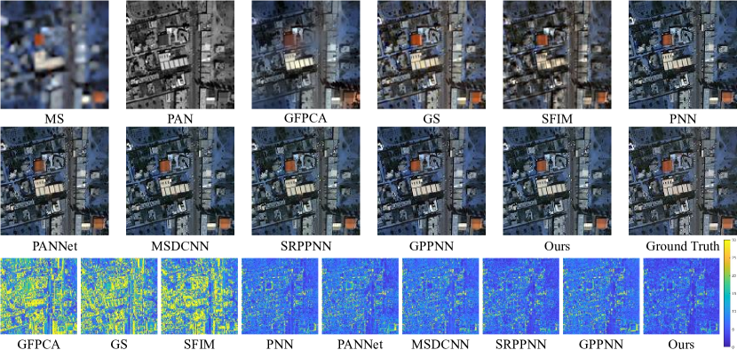
Figure 2: Qualitative visualization comparison of our method with other representative counterparts on a typical satellite image pair from the WordView-III dataset. Images in the last row visualizes the MSE between the fused images and the ground truth.

Results on Real-world Full-resolution Scene

To assess the generalization performance of models in real-world scene, we apply models trained on the GF2 dataset to additional 200 paired GaoFen2 satellite images which are constructed using the full-resolution setting as the real scene. Lacking available ground-truth at full-resolution scene, we employ three widely-used non-reference metrics for assessing the performance: $D_{\lambda}$, $D_{S}$ and QNR. The quantitative and qualitative results are summarized in Table 2 and Figure 3 that clearly demonstrate the higher generalization capacity of the proposed alternating reverse filtering network.

Table 2: The average quantitative results on the GaoFen2 datasets on the real-world full-resolution scene. The best results are highlighted by bold.

Metrics	SFIM	GS	Brovey	IHS	GFPCA	PNN	PANNET	MSDCNN	SRPPNN	GPPNN	Ours
$D_{\lambda}\downarrow$	0.0822	0.0696	0.1378	0.0770	0.0914	0.0746	0.0737	0.0734	0.0767	0.0782	0.0635
$D_{s}\downarrow$	0.1087	0.2456	0.2605	0.2985	0.1635	0.1164	0.1224	0.1151	0.1162	0.1253	0.1156
$QNR\uparrow$	0.8214	0.7025	0.6390	0.6485	0.7615	0.8191	0.8143	0.8215	0.8173	0.8073	0.8237

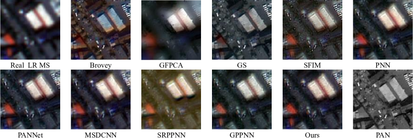
Figure 3: Qualitative visualization comparison of our method with other representative methods over real-world full-resolution scenes.

4.3 Ablation Study

Ablation studies are implemented on the WordView-II dataset to explore the effect of different parameters and components on the performance of models. We use the ARFNet in subsection 4.1 as the baseline for comparison by changing parameters and components, and all comparison models are trained in the same way. Firstly, to balance the overall performance and the structure details, we fix the other components and change only the value of the hyperparameter $\lambda$. The results in Table 3 show that the larger the value of $\lambda$ is within a certain range, the higher the structure similarity between the fused image and ground truth will be. Note that if the reverse filtering network $\varphi_{2}(\cdot)$ lack the supervision $\mathcal{L}_{s}$ that the performance of the entire network will be a significant decrease.

Table 3: The effect of hyperparameter $\lambda$ in loss function $\mathcal{L}_{sum}$.

$\lambda$	0	0.001	0.01	0.1	0.5	1	2
PSNR$\uparrow$	40.1274	40.8279	41.3267	41.7587	41.6932	41.2736	41.0746
SSIM$\uparrow$	0.9598	0.9630	0.9673	0.9691	0.9694	0.9664	0.9653
SAM$\downarrow$	0.0264	0.0256	0.0242	0.0229	0.0232	0.247	0.0260
ERGAS$\downarrow$	1.0677	1.0561	0.9943	0.9540	0.9564	1.0037	1.0491

Furthermore, we compare the results of different initialization methods. In Table 4, (I) represents the kernels that are randomly initialized by Kaiming [70], (II) and (III) represents the kernels that are initialized by Gaussian kernels, but the kernels in (III) are fixed. From Table 4 and Figure 4, one could see that: 1) The kernels learned by the randomly initialized network cannot satisfy the sufficient condition, which leads to poor performance. 2) The learned kernels initialized by Gaussian kernels are close to the kernels we initialize, that makes $\{\mathbf{H}_{c}^{k}\}$ the majority and dominates the convergence of the whole process. 3) Although the learned kernels are close to the initialized Gaussian kernels, a large number of multi-scale Gaussian kernels can still bring performance improvements.

Table 4: Quantitative comparison of different initialization methods on the WorldView-II dataset.

Methods	PSNR$\uparrow$	SSIM$\uparrow$	SAM$\downarrow$	ERGAS$\downarrow$	SCC$\uparrow$	Q$\uparrow$	$D_{\lambda}\downarrow$	$D_{S}\downarrow$	QNR$\uparrow$
(I)	40.3297	0.9601	0.0262	1.0672	0.9663	0.7310	0.0698	0.1277	0.8097
(II)	41.7587	0.9691	0.0229	0.9540	0.9749	0.7731	0.0631	0.1184	0.8285
(III)	40.4161	0.9612	0.0261	1.0668	0.9667	0.7316	0.0684	0.1275	0.8123

Initialized random kernels				Learned kernels (initialized by random kernels)
$3\times 3$	$7\times 7$	$13\times 13$	$17\times 17$	$3\times 3$	$7\times 7$	$13\times 13$	$17\times 17$
Initialized Gaussian kernels				Learned kernels (initialized by Gaussian kernels)
$3\times 3$	$7\times 7$	$13\times 13$	$17\times 17$	$3\times 3$	$7\times 7$	$13\times 13$	$17\times 17$

Figure 4: Visualization of initialized kernels and learned kernels.

As can be seen from Table 5, the ablation studies about maximum kernel size $M$ show that the multi-scale Gaussian convolution module can bring better performance improvement. To explore the impact of the number of iterations $K$ on the performance, we experiment with varying numbers of $K$. Table 6 shows the results of different $K$ from 1 to 7. It can be seen that the PSNR performance increases as the number of stages increases. We choose $K=5$ in our implementation to balance the performance and computational complexity.

Table 5: The comparison results of ablation study about maximum kernel size $M$.

$M$	1	3	5	7	9	11	13	15	17	19	21
PSNR$\uparrow$	39.7820	40.6804	41.0634	41.4371	41.5297	41.6445	41.6910	41.7252	41.7587	41.7126	41.6982
SSIM$\uparrow$	0.9584	0.9603	0.9657	0.9665	0.9679	0.9684	0.9688	0.9690	0.9691	0.9689	0.9683

Table 6: The comparison results of ablation study about the number of iterations $K$.

$K$	1	2	3	4	5	6	7
PSNR$\uparrow$	40.7130	41.056	41.3927	41.6869	41.7587	41.7614	41.7603
SSIM$\uparrow$	0.9611	0.9654	0.9667	0.9684	0.9691	0.9690	0.9688

4.4 Limitations and Discussions

First, we evaluate the effectiveness of the proposed framework over panchromatic and multispectral image fusion and we will extend the framework to other multispectral fusion tasks, such as RGB and multispectral image fusion. Second, although we develop the multi-scale Gaussian kernel module to ensure the convergence of the alternating reverse filtering, there is still a large room to explore a learnable filter function that can strictly satisfy sufficient conditions.

5 Conclusion

In this paper, we presented a simple yet effective alternating reverse filtering network for pan-sharpening. The proposed approach formulates pan-sharpening as a reverse filtering process and combines classical reverse filtering and deep learning. The classical reverse filtering is unrolled to a network without pre-defined exact priors in an alternating iteration manner. Besides, multi-scale Gaussian kernel module is developed to ensure the convergence of the iterative process. Furthermore, the ablation studies verified the effectiveness of the multi-scale Gaussian kernel module. Extensive experimental results on simulated and real-world scenes show that the proposed network significantly outperforms the state of the arts. In the future, we will study the extension to other image fusion problems such as RGB and multispectral image fusion.

Broader Impact

This research aims to address the problem of panchromatic and multispectral image fusion, which is a key pre-processing technology overcoming the constraints of hardware before using high-resolution multispectral image. The fused multispectral images are needed as a reference in the field of resource monitoring, such as land use planning, ocean development, and urban management, and in the field of ecological and environmental protection areas, such as pollution monitoring, vegetation biology and precision agriculture research. Despite the many benefits of fused multispectral images, negative consequences can still occur in several special environments. When there is a case of algorithm failure, artifacts generated on the fusion image may affect subsequent use and lead to misjudgments.

References

Checklist

1. For all authors…

   1. Do the main claims made in the abstract and introduction accurately reflect the paper’s contributions and scope? [Yes]

   2. Did you describe the limitations of your work? [Yes] , see Section 4.4.

   3. Did you discuss any potential negative societal impacts of your work? [Yes] , see Section Broader Impact.

   4. Have you read the ethics review guidelines and ensured that your paper conforms to them? [Yes]

2. If you are including theoretical results…

   1. Did you state the full set of assumptions of all theoretical results? [Yes] , See Section 3.2 and Section 3.3.

   2. Did you include complete proofs of all theoretical results? [Yes] , See Section 3.2 and Section 3.3.

3. If you ran experiments…

   1. Did you include the code, data, and instructions needed to reproduce the main experimental results (either in the supplemental material or as a URL)? [Yes] , Instructions about experimental settings are in Section 4.1, and the URL of the project will be released after the paper is accepted.

   2. Did you specify all the training details (e.g., data splits, hyperparameters, how they were chosen)? [Yes]

   3. Did you report error bars (e.g., with respect to the random seed after running experiments multiple times)? [No] , the effect of random seed could almost be negligible since we set the same initiation seed during experiments. Reproducibility can be guaranteed.

   4. Did you include the total amount of compute and the type of resources used (e.g., type of GPUs, internal cluster, or cloud provider)? [Yes]

4. If you are using existing assets (e.g., code, data, models) or curating/releasing new assets…

   1. If your work uses existing assets, did you cite the creators? [Yes]

   2. Did you mention the license of the assets? [Yes]

   3. Did you include any new assets either in the supplemental material or as a URL? [Yes]

   4. Did you discuss whether and how consent was obtained from people whose data you’re using/curating? [Yes] , the data creators claim that they allow and encourage the data for scientific research.

   5. Did you discuss whether the data you are using/curating contains personally identifiable information or offensive content? [N/A] , We train and test the framework using the datasets following the prior works.

5. If you used crowdsourcing or conducted research with human subjects…

   1. Did you include the full text of instructions given to participants and screenshots, if applicable? [N/A]

   2. Did you describe any potential participant risks, with links to Institutional Review Board (IRB) approvals, if applicable? [N/A]

   3. Did you include the estimated hourly wage paid to participants and the total amount spent on participant compensation? [N/A]

References

- [1] Xiangchao Meng, Huanfeng Shen, Huifang Li, Liangpei Zhang, and Randi Fu. Review of the pansharpening methods for remote sensing images based on the idea of meta-analysis: Practical discussion and challenges. Information Fusion, 46:102–113, 2019.
- [2] Farzaneh Dadrass Javan, Farhad Samadzadegan, Soroosh Mehravar, Ahmad Toosi, Reza Khatami, and Alfred Stein. A review of image fusion techniques for pan-sharpening of high-resolution satellite imagery. ISPRS Journal of Photogrammetry and Remote Sensing, 171:101–117, 2021.
- [3] Yong Yang, Hangyuan Lu, Shuying Huang, and Wei Tu. Remote sensing image fusion based on fuzzy logic and salience measure. IEEE Geoscience and Remote Sensing Letters, 17(11):1943–1947, 2020.
- [4] Yanfeng Gu, Tianzhu Liu, Guoming Gao, Guangbo Ren, Yi Ma, Jocelyn Chanussot, and Xiuping Jia. Multimodal hyperspectral remote sensing: an overview and perspective. Science China Information Sciences, 64, 02 2021.
- [5] Gemine Vivone, Stefano Marano, and Jocelyn Chanussot. Pansharpening: Context-based generalized laplacian pyramids by robust regression. IEEE Transactions on Geoscience and Remote Sensing, 58(9):6152–6167, 2020.
- [6] Yuxuan Zheng, Jiaojiao Li, Yunsong Li, Jie Guo, Xianyun Wu, and Jocelyn Chanussot. Hyperspectral pansharpening using deep prior and dual attention residual network. IEEE Transactions on Geoscience and Remote Sensing, 58(11):8059–8076, 2020.
- [7] Lin He, Jiawei Zhu, Jun Li, Deyu Meng, Jocelyn Chanussot, and Antonio Plaza. Spectral-fidelity convolutional neural networks for hyperspectral pansharpening. IEEE Journal of Selected Topics in Applied Earth Observations and Remote Sensing, 13:5898–5914, 2020.
- [8] Liang-Jian Deng, Gemine Vivone, Cheng Jin, and Jocelyn Chanussot. Detail injection-based deep convolutional neural networks for pansharpening. IEEE Transactions on Geoscience and Remote Sensing, 59(8):6995–7010, 2021.
- [9] Giuseppe Masi, Davide Cozzolino, Luisa Verdoliva, and Giuseppe Scarpa. Pansharpening by convolutional neural networks. Remote Sensing, 8(7), 2016.
- [10] Peng Wang, Lei Zhang, Gong Zhang, Hui Bi, Mauro Dalla Mura, and Jocelyn Chanussot. Superresolution land cover mapping based on pixel-, subpixel-, and superpixel-scale spatial dependence with pansharpening technique. IEEE Journal of Selected Topics in Applied Earth Observations and Remote Sensing, 12(10):4082–4098, 2019.
- [11] P Kwarteng and A Chavez. Extracting spectral contrast in landsat thematic mapper image data using selective principal component analysis. Photogrammetric Engineering and remote sensing, 55(339-348):1, 1989.
- [12] Sheida Rahmani, Melissa Strait, Daria Merkurjev, Michael Moeller, and Todd Wittman. An adaptive ihs pan-sharpening method. IEEE Geoscience and Remote Sensing Letters, 7(4):746–750, 2010.
- [13] Muhammad Murtaza Khan, Jocelyn Chanussot, Laurent Condat, and Annick Montanvert. Indusion: Fusion of multispectral and panchromatic images using the induction scaling technique. IEEE Geoscience and Remote Sensing Letters, 5(1):98–102, 2008.
- [14] Gemine Vivone, Luciano Alparone, Jocelyn Chanussot, Mauro Dalla Mura, Andrea Garzelli, Giorgio A. Licciardi, Rocco Restaino, and Lucien Wald. A critical comparison among pansharpening algorithms. IEEE Transactions on Geoscience and Remote Sensing, 53(5):2565–2586, 2015.
- [15] Xueyang Fu, Zihuang Lin, Yue Huang, and Xinghao Ding. A variational pan-sharpening with local gradient constraints. In Proceedings of the IEEE/CVF Conference on Computer Vision and Pattern Recognition, pages 10265–10274, 2019.
- [16] Xin Tian, Yuerong Chen, Changcai Yang, and Jiayi Ma. Variational pansharpening by exploiting cartoon-texture similarities. IEEE Transactions on Geoscience and Remote Sensing, pages 1–16, 2021.
- [17] Theo Bodrito, Alexandre Zouaoui, Jocelyn Chanussot, and Julien Mairal. A trainable spectral-spatial sparse coding model for hyperspectral image restoration. Adv. in Neural Information Processing Systems (NeurIPS), 2021.
- [18] Keiller Nogueira, Mauro Dalla Mura, Jocelyn Chanussot, William Robson Schwartz, and Jefersson Alex dos Santos. Dynamic multicontext segmentation of remote sensing images based on convolutional networks. IEEE Transactions on Geoscience and Remote Sensing, 57(10):7503–7520, 2019.
- [19] Gemine Vivone, Paolo Addesso, Rocco Restaino, Mauro Dalla Mura, and Jocelyn Chanussot. Pansharpening based on deconvolution for multiband filter estimation. IEEE Transactions on Geoscience and Remote Sensing, 57(1):540–553, 2019.
- [20] Lin He, Jiawei Zhu, Jun Li, Antonio Plaza, Jocelyn Chanussot, and Bo Li. Hyperpnn: Hyperspectral pansharpening via spectrally predictive convolutional neural networks. IEEE Journal of Selected Topics in Applied Earth Observations and Remote Sensing, 12(8):3092–3100, 2019.
- [21] Man Zhou, Xueyang Fu, Jie Huang, Feng Zhao, Aiping Liu, and Rujing Wang. Effective pan-sharpening with transformer and invertible neural network. IEEE Transactions on Geoscience and Remote Sensing, 60:1–15, 2022.
- [22] Man Zhou, Keyu Yan, Jie Huang, Zihe Yang, Xueyang Fu, and Feng Zhao. Mutual information-driven pan-sharpening. In 2022 IEEE/CVF Conference on Computer Vision and Pattern Recognition, pages 1788–1798, 2022.
- [23] Kai Zhang, Luc Van Gool, and Radu Timofte. Deep unfolding network for image super-resolution. In Proceedings of the IEEE/CVF Conference on Computer Vision and Pattern Recognition, pages 3217–3226, 2020.
- [24] Shuang Xu, Jiangshe Zhang, Zixiang Zhao, Kai Sun, Junmin Liu, and Chunxia Zhang. Deep gradient projection networks for pan-sharpening. In IEEE Conference on Computer Vision and Pattern Recognition, pages 1366–1375, June 2021.
- [25] Xin Tao, Chao Zhou, Xiaoyong Shen, Jue Wang, and Jiaya Jia. Zero-order reverse filtering. In 2017 IEEE International Conference on Computer Vision (ICCV), pages 222–230, 2017.
- [26] Xin Tian, Yuerong Chen, Changcai Yang, Xun Gao, and Jiayi Ma. A variational pansharpening method based on gradient sparse representation. IEEE Signal Processing Letters, 27:1180–1184, 2020.
- [27] Behnood Rasti, Pedram Ghamisi, and Richard Gloaguen. Hyperspectral and lidar fusion using extinction profiles and total variation component analysis. IEEE Transactions on Geoscience and Remote Sensing, 55(7):3997–4007, 2017.
- [28] Behnood Rasti, Magnus Orn Ulfarsson, and Johannes R. Sveinsson. Hyperspectral feature extraction using total variation component analysis. IEEE Transactions on Geoscience and Remote Sensing, 54(12):6976–6985, 2016.
- [29] Behnood Rasti, Johannes R. Sveinsson, and Magnus O. Ulfarsson. Total variation based hyperspectral feature extraction. In 2014 IEEE Geoscience and Remote Sensing Symposium, pages 4644–4647, 2014.
- [30] Wjoseph Carper, Thomasm Lillesand, and Ralphw Kiefer. The use of intensity-hue-saturation transformations for merging spot panchromatic and multispectral image data. Photogrammetric Engineering and remote sensing, 56(4):459–467, 1990.
- [31] Vijay P. Shah, Nicolas H. Younan, and Roger L. King. An efficient pan-sharpening method via a combined adaptive pca approach and contourlets. IEEE Transactions on Geoscience and Remote Sensing, 46(5):1323–1335, 2008.
- [32] Alan R Gillespie, Anne B Kahle, and Richard E Walker. Color enhancement of highly correlated images. ii. channel ratio and "chromaticity" transformation techniques. Remote Sensing of Environment, 22(3):343–365, 1987.
- [33] Craig A Laben and Bernard V Brower. Process for enhancing the spatial resolution of multispectral imagery using pan-sharpening, 2000. US Patent 6,011,875.
- [34] SG Mallat. A theory for multiresolution signal decomposition: The wavelet representation. IEEE Transactions on Pattern Analysis and Machine Intelligence, 11(7):674–693, 1989.
- [35] Robert A Schowengerdt. Reconstruction of multispatial, multispectral image data using spatial frequency content. Photogrammetric Engineering and Remote Sensing, 46(10):1325–1334, 1980.
- [36] Jorge Nunez, Xavier Otazu, Octavi Fors, Albert Prades, Vicenc Pala, and Roman Arbiol. Multiresolution-based image fusion with additive wavelet decomposition. IEEE Transactions on Geoscience and Remote sensing, 37(3):1204–1211, 1999.
- [37] Chen Chen, Yeqing Li, Wei Liu, and Junzhou Huang. Sirf: Simultaneous satellite image registration and fusion in a unified framework. IEEE Transactions on Image Processing, 24(11):4213–4224, 2015.
- [38] Junfeng Yang, Xueyang Fu, Yuwen Hu, Yue Huang, Xinghao Ding, and John Paisley. Pannet: A deep network architecture for pan-sharpening. In IEEE International Conference on Computer Vision, pages 5449–5457, 2017.
- [39] Man Zhou, Xueyang Fu, Jie Huang, Feng Zhao, Aiping Liu, and Rujing Wang. Effective pan-sharpening with transformer and invertible neural network. IEEE Transactions on Geoscience and Remote Sensing, 60:1–15, 2022.
- [40] Kaiming He, Xiangyu Zhang, Shaoqing Ren, and Jian Sun. Deep residual learning for image recognition. In IEEE Conference on Computer Vision and Pattern Recognition, pages 770–778, 2016.
- [41] Qiangqiang Yuan, Yancong Wei, Xiangchao Meng, Huanfeng Shen, and Liangpei Zhang. A multiscale and multidepth convolutional neural network for remote sensing imagery pan-sharpening. IEEE Journal of Selected Topics in Applied Earth Observations and Remote Sensing, 11(3):978–989, 2018.
- [42] Weisheng Dong, Peiyao Wang, Wotao Yin, Guangming Shi, Fangfang Wu, and Xiaotong Lu. Denoising prior driven deep neural network for image restoration. IEEE transactions on pattern analysis and machine intelligence, 41(10):2305–2318, 2018.
- [43] Risheng Liu, Zhiying Jiang, Xin Fan, and Zhongxuan Luo. Knowledge-driven deep unrolling for robust image layer separation. IEEE transactions on neural networks and learning systems, 31(5):1653–1666, 2019.
- [44] Risheng Liu, Long Ma, Yuxi Zhang, Xin Fan, and Zhongxuan Luo. Underexposed image correction via hybrid priors navigated deep propagation. IEEE Transactions on Neural Networks and Learning Systems, 2021.
- [45] Kai Zhang, Wangmeng Zuo, Shuhang Gu, and Lei Zhang. Learning deep cnn denoiser prior for image restoration. In Proceedings of the IEEE conference on computer vision and pattern recognition, pages 3929–3938, 2017.
- [46] Xiangyong Cao, Xueyang Fu, Danfeng Hong, Zongben Xu, and Deyu Meng. Pancsc-net: A model-driven deep unfolding method for pansharpening. IEEE Transactions on Geoscience and Remote Sensing, pages 1–13, 2021.
- [47] Jian Zhang Jiechong Song, Bin Chen. Memory-augmented deep unfolding network for compressive sensing. In ACM International Conference on Multimedia (ACM MM), 2021.
- [48] Manya V Afonso, José M Bioucas-Dias, and Mário AT Figueiredo. Fast image recovery using variable splitting and constrained optimization. IEEE transactions on image processing, 19(9):2345–2356, 2010.
- [49] Xueyang Fu, Zheng-Jun Zha, Feng Wu, Xinghao Ding, and John Paisley. Jpeg artifacts reduction via deep convolutional sparse coding. In Proceedings of the IEEE/CVF International Conference on Computer Vision, pages 2501–2510, 2019.
- [50] Dror Simon and Michael Elad. Rethinking the CSC model for natural images. In NeurIPS, pages 2271–2281, 2019.
- [51] Liang Chen, Jiawei Zhang, Jinshan Pan, Songnan Lin, Faming Fang, and Jimmy S. Ren. Learning a non-blind deblurring network for night blurry images. In Proceedings of the IEEE/CVF Conference on Computer Vision and Pattern Recognition (CVPR), pages 10542–10550, June 2021.
- [52] Shuang Xu, Ouafa Amira, Junmin Liu, Chun-Xia Zhang, Jiangshe Zhang, and Guanghai Li. Ham-mfn: Hyperspectral and multispectral image multiscale fusion network with rap loss. IEEE Transactions on Geoscience and Remote Sensing, 58(7):4618–4628, 2020.
- [53] Shuang Xu, Lizhen Ji, Zhe Wang, Pengfei Li, Kai Sun, Chunxia Zhang, and Jiangshe Zhang. Towards reducing severe defocus spread effects for multi-focus image fusion via an optimization based strategy. IEEE Transactions on Computational Imaging, 6:1561–1570, 2020.
- [54] Risheng Liu, Long Ma, Jiaao Zhang, Xin Fan, and Zhongxuan Luo. Retinex-inspired unrolling with cooperative prior architecture search for low-light image enhancement. In Proceedings of the IEEE/CVF Conference on Computer Vision and Pattern Recognition (CVPR), pages 10561–10570, June 2021.
- [55] Risheng Liu, Yuxi Zhang, Shichao Cheng, Zhongxuan Luo, and Xin Fan. A deep framework assembling principled modules for cs-mri: Unrolling perspective, convergence behaviors, and practical modeling. IEEE Transactions on Medical Imaging, 39(12):4150–4163, 2020.
- [56] Risheng Liu, Zhiying Jiang, Xin Fan, and Zhongxuan Luo. Knowledge-driven deep unrolling for robust image layer separation. IEEE Trans. Neural Networks Learn. Syst., 31(5):1653–1666, 2020.
- [57] Yang Liu, Jinshan Pan, Jimmy S. J. Ren, and Zhixun Su. Learning deep priors for image dehazing. In 2019 IEEE/CVF International Conference on Computer Vision, ICCV 2019, Seoul, Korea (South), October 27 - November 2, 2019, pages 2492–2500. IEEE, 2019.
- [58] Wen Dou, Yunhao Chen, Xiaobing Li, and Daniel Z. Sui. A general framework for component substitution image fusion: An implementation using the fast image fusion method. Computers & Geosciences, 33(2):219–228, 2007.
- [59] S Banach. Surles operation dans ensembles abstraits etleur application aux equations integrals, fund, 1922.
- [60] Yuhui Quan, Zicong Wu, and Hui Ji. Gaussian kernel mixture network for single image defocus deblurring. In M. Ranzato, A. Beygelzimer, Y. Dauphin, P.S. Liang, and J. Wortman Vaughan, editors, Advances in Neural Information Processing Systems, volume 34, pages 20812–20824. Curran Associates, Inc., 2021.
- [61] Lucien Wald, Thierry Ranchin, and Marc Mangolini. Fusion of satellite images of different spatial resolutions: Assessing the quality of resulting images. Photogrammetric Engineering and Remote Sensing, 63:691–699, 11 1997.
- [62] J. G. Liu. Smoothing filter-based intensity modulation: A spectral preserve image fusion technique for improving spatial details. International Journal of Remote Sensing, 21(18):3461–3472, 2000.
- [63] R. Haydn, G. W. Dalke, J. Henkel, and J. E. Bare. Application of the ihs color transform to the processing of multisensor data and image enhancement. National Academy of Sciences of the United States of America, 79(13):571–577, 1982.
- [64] W. Liao, H. Xin, F. V. Coillie, G. Thoonen, and W. Philips. Two-stage fusion of thermal hyperspectral and visible rgb image by pca and guided filter. In Workshop on Hyperspectral Image and Signal Processing: Evolution in Remote Sensing, 2017.
- [65] Jiajun Cai and Bo Huang. Super-resolution-guided progressive pansharpening based on a deep convolutional neural network. IEEE Transactions on Geoscience and Remote Sensing, 59(6):5206–5220, 2021.
- [66] Shuang Xu, Jiangshe Zhang, Zixiang Zhao, Kai Sun, Junmin Liu, and Chunxia Zhang. Deep gradient projection networks for pan-sharpening. In CVPR, pages 1366–1375, June 2021.
- [67] L. Alparone, L. Wald, J. Chanussot, C. Thomas, P. Gamba, and L. M. Bruce. Comparison of pansharpening algorithms: Outcome of the 2006 grs-s data fusion contest. IEEE Transactions on Geoscience and Remote Sensing, 45(10):3012–3021, 2007.
- [68] Roberta H. Yuhas, Alexander F. H. Goetz, and Joseph W. Boardman. Discrimination among semi-arid landscape endmembers using the spectral angle mapper (sam) algorithm. Proc. Summaries Annu. JPL Airborne Geosci. Workshop, pages 147–149, 1992.
- [69] Luciano Alparone, Bruno Aiazzi, Stefano Baronti, Andrea Garzelli, Filippo Nencini, and Massimo Selva. Multispectral and panchromatic data fusion assessment without reference. Photogrammetric Engineering & Remote Sensing, 74(2):193–200, 2008.
- [70] Kaiming He, Xiangyu Zhang, Shaoqing Ren, and Jian Sun. Delving deep into rectifiers: Surpassing human-level performance on imagenet classification. In 2015 IEEE International Conference on Computer Vision (ICCV), pages 1026–1034, 2015.