Attention Regularized Laplace Graph for Domain Adaptation

Abstract

In leveraging manifold learning in domain adaptation (DA), graph embedding-based DA methods have shown their effectiveness in preserving data manifold through the Laplace graph. However, current graph embedding DA methods suffer from two issues: 1). they are only concerned with preservation of the underlying data structures in the embedding and ignore sub-domain adaptation, which requires taking into account intra-class similarity and inter-class dissimilarity, thereby leading to negative transfer; 2). manifold learning is proposed across different feature/label spaces separately, thereby hindering unified comprehensive manifold learning. In this paper, starting from our previous DGA-DA, we propose a novel DA method, namely Attention Regularized Laplace Graph-based Domain Adaptation (ARG-DA), to remedy the aforementioned issues. Specifically, by weighting the importance across different sub-domain adaptation tasks, we propose the Attention Regularized Laplace Graph for class aware DA, thereby generating the attention regularized DA. Furthermore, using a specifically designed FEEL strategy, our approach dynamically unifies alignment of the manifold structures across different feature/label spaces, thus leading to comprehensive manifold learning. Comprehensive experiments are carried out to verify the effectiveness of the proposed DA method, which consistently outperforms the state of the art DA methods on 7 standard DA benchmarks, i.e., 37 cross-domain image classification tasks including object, face, and digit images. An in-depth analysis of the proposed DA method is also discussed, including sensitivity, convergence, and robustness.

I Introduction

Supervised learning was at the forefront of increasing real-world applications within the big data era [61, 63, 71, 54]. However, its success relied greatly on the availability of large amounts of high-quality labeled data and assumed that training and testing data share the same distribution for the effectiveness of the learned model. Unfortunately, in real-life applications, data distribution shifts, due to factors as diverse as environment variations, e.g., lighting, temperature, differences in data capture devices, etc., frequently (though not always) occur. It is thus of capital importance to guarantee that a learned model using a given set of training data, namely the source domain, remains effective on a set of testing data, namely the target domain, despite data distribution shifts. This is precisely the objective of the research field of domain adaptation (DA), which aims to develop theories and techniques for effective learning algorithms, while making use of previously labeled data (source domain) and unlabeled data in the current task (target domain), despite the distribution divergence.

While DA can be semi-supervised by assuming a certain amount of labeled data are available in the target domain, in this paper we are interested in unsupervised DA where we assume that the target domain has no labels. While there also exists an increasing number of deep learning-based unsupervised DA methods, here we focus on shallow DA methods as they are easier to train and can provide insights into the design decisions of deep DA methods. The relationships between shallow and deep DA methods will be further discussed in depth in Sect.II on related works.

State-of-the-art shallow DA methods can be categorized into instance-based [61, 12], feature-based [62, 50, 88], or classifier-based. Classifier-based DA is widely applied in semi-supervised DA as it aims to fit a classifier trained on the source domain data to target domain data through adaptation of its parameters, thereby requiring some labels in the target domain [77]. The instance-based approach generally assumes that 1) the conditional distributions of the source and target domains are identical [91], and 2) a certain portion of the data in the source domain can be reused [61] for learning in the target domain through re-weighting. Feature-based adaptation [75, 25, 16, 78, 55] relaxes such a strict assumption and only requires that there exists a mapping from the input data space to a latent shared feature representation space. This latent shared feature space captures the information necessary for training classifiers for both source and target tasks. In this paper, we propose a novel feature-based DA method, which searches a latent feature space using the Laplace graph, but which is regularized by class aware attention along with a unified manifold alignment framework for an effective DA.

A common method for approaching feature adaptation is to seek a shared latent subspace between the source and target domains via optimization [63, 62]. State-of-the-art features three main lines of approach, namely, data geometric structure alignment-based (DGSA), data distribution centered (DDC) or their hybridization. DDC methods [55, 52, 45, 53] aim to search a latent subspace where the discrepancy between the source and target data distributions is minimized, via various distances, e.g., Bregman divergence [74], Geodesic distance [18], Wasserstein distance [7, 8] or Maximum Mean Discrepancy [22] (MMD). DGSA-based methods seek to align the underlying data geometric structures and can be further categorized into subspace alignment-based DA (DGSA-SA DA) and graph embedding-based DA (DGSA-GE DA). DGSA-SA methods, e.g., [75, 72, 88], aim to align different feature spaces under the reconstruction framework using the low rank constraint and/or sparse representation, while DGSA-GE methods explicitly model the underlying data geometric structure by using Laplace graph representation-based manifold learning, thereby seeking a subspace where the source and target data can be well aligned and interleaved by preserving inherent hidden geometric data structures. By hybridizing the DGSA-GE and DDC approaches, our proposed method, namely ARG-DA, strives to leverage the merits of simultaneous alignment of both data distributions and the underlying data geometric structures between the source and target domains.

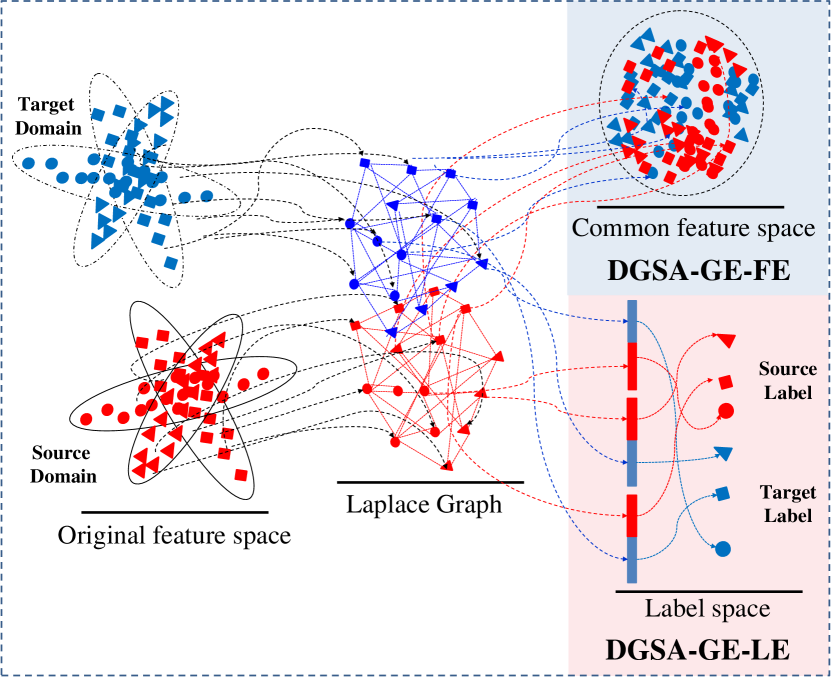
Figure 1: Illustration of difference across the Feature space Embedding-based DA (DGSA-GE-FE) and the Label space Embedding-based DA (DGSA-GE-LE).

Popular DGSA-GE methods align different feature/label spaces using graph embedding techniques and can be further summarized into two main research lines, namely feature space embedding-based DA (DGSA-GE-FE), e.g., [33, 92], and label space embedding-based DA (DGSA-GE-LE), e.g., [93, 44, 55]. As shown in Fig.1, DGSA-GE-FE methods seek a common feature space between the source and the target domain by preserving the underlying data geometric structure, while DGSA-GE-LE methods enforce the alignment of manifold structures across the feature space and the label space.

To gain insights into both DGSA-GE-FE and DGSA-GE-LE methods, we review the cornerstone theoretical result in DA [2, 34], which estimates an error bound of a learned hypothesis $h$ on a target domain as follows:

where ${e_{\cal S}}(h)$ denotes the classification error on the source domain, and ${{d_{\cal H}}({{\cal D}_{\cal S}},{{\cal D}_{\cal T}})}$ measures the $\mathcal{H}$-divergence [34] between two distributions ($\mathcal{D_{S}}$, $\mathcal{D_{T}}$) of the source and target domain. The last term of Eq.(1) represents the difference in labeling functions across the two domains. Following Eq.(1), both the DGSA-GE-FE and DGSA-GE-LE methods are concerned with manifold structure preservation, which potentially shrinks the divergence between different labeling functions proposed on the two domains, thereby reducing term.3 of Eq.(1). Different from DGSA-GE-FE, DGSA-GE-LE methods further leverage the discriminative power induced by the labels available on the source domain data by aligning the underlying data geometric structure in accordance with the data labels, thereby reducing the classification error on the source domain ${e_{\cal S}}(h)$ (term.1). However, despite interesting performance enabled DGSA-GE methods, they still suffer from the following two issues:

Lack of Attention: The attention mechanism refers to pooling a sequence or a set of features with different weights in order to compute proper representation of the whole sequence or set [81, 29], thereby making it possible to deal differently with different data features while aggregating. However, by enforcing the maintenance of the geometric structure of the underlying data manifold while searching a joint feature subspace between the source and target domains, Laplace graph-based embedding DA methods, i.e., DGSA-GE methods, treat equally all the sub-domain adaptations and can lead to cross-domain misalignment as shown in Fig.2. As can be seen, Fig.2.(b,d) depicts the two-dimensional embeddings from their original three-dimensional feature space as shown in Fig.2.(a,c), respectively.

• P1: Fig.2.(b) preserves the data geometric structure of the original data space as in Fig.2.(a) but as a result fails to close adaptatively the corresponding sub-domains, e.g., ’1’, since the two sub-domains (’1’) are distant in the original data manifold as depicted in Fig.2.(a).

• P2: Fig.2.(d) succeeds in aligning the data manifold structures with respect to their original data space as in Fig.2.(c), but as a result fails to separate the two sub-domains, namely, ’1’ and ’3’, which are geometrically close in the original data space.

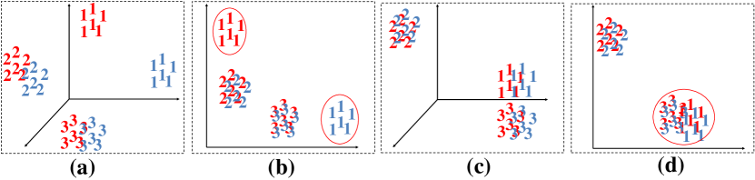
Figure 2: Fig.2.(a,c) represents the feature representation in its original three-dimensional feature space; Fig.2.(b,d) represents the feature representation in its two-dimensional common feature space by DGSA-GE; red and blue samples represent the source and target domains, while the numbers ’1’, ’2’, and ’3’ denote three different classes or sub-domains, respectively.

The failures of P1 and P2 are due to the fact that traditional graph embedding-based manifold learning only seeks to preserve the relative distances across different feature spaces. However, solving a DA task requires bringing closer intra sub-domains across domains, while increasing the relative distances of inter sub-domains in the novel projected feature space. As a result, in this paper we propose a novel discriminativeness aware graph embedding, namely, Attention Regularized Graph (ARG), to remedy the aforementioned issues as highlighted by P1 and P2.

Incomplete Unification: by aligning the manifold structures across different feature spaces, DGSA-GE-FE methods harness the geometric knowledge transferred across feature spaces, but fail to leverage the discriminative power induced by the labels available in the source domain data. On the other hand, DGSA-GE-LE remedies the previous issue and unifies the manifold structure across the feature space and the label space for label inference, but fails to align the geometric structures across different feature spaces [19] to ensure smooth transfer learning between the source and target domains. Therefore, a hybridization of both DGSA-GE-FE and DGSA-GE-LE can be appealing for comprehensive manifold learning enhanced DA to leverage the advantages of both approaches.

In this paper, we propose a novel DA method, namely, Attention Regularized Laplace Graph-based Domain Adaptation (ARG-DA), to address the aforementioned ’Lack of Attention’ and ’Incomplete Unification’ issues. Specifically, the proposed (ARG-DA), 1) optimizes the Attention Regularized Laplace Graph guided by MMD-based distribution measurements over cross-domain sub-tasks, thereby enforcing the attention regularized manifold learning and 2) implements a hybridization strategy, namely, ’FEEL’, to unify the manifold structure across the feature/label spaces for comprehensive manifold alignment.

To conclude, the contributions of this paper are summarized as follows:

• The Attention Regularized Laplace Graph is designed to enable discriminative manifold embedding, guided by MMD-based distribution measurements over cross-domain sub-tasks, thereby reducing negative transfer.

• A comprehensive manifold unification strategy, namely, FEEL, is proposed for comprehensive manifold learning, which aligns the manifold structure across different feature spaces to minimize term.3 of Eq.(1), while enforcing the alignment across feature space and label space so as to reduce term.1 of Eq.(1).

• We carry out extensive experiments on 37 image classification DA tasks through 7 popular DA benchmarks and verify the effectiveness of the proposed method, which consistently outperforms thirty-three state-of-the-art DA algorithms by a significant margin. Moreover, we also carry out an in-depth analysis of the proposed DA methods, in particular, w.r.t. their hyper-parameters and convergence speed. In addition, using real data, we also provide insights into the proposed DA model by analyzing the robustness of our proposed ARG term and FEEL strategy.

The paper is organized as follows. Sect.II discusses the related work. Sect.III presents the method. Sect.IV benchmarks the proposed DA method and provides an in-depth analysis. Sect.V draws the conclusion.

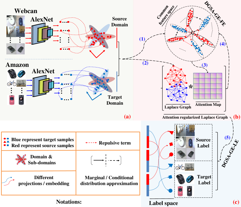
Figure 3: Illustration of the proposed ARG-DA method. Fig.3 (a): source data and target data, e.g., mouse, bike, smartphone images, with different distributions and inherent hidden data geometric structures between the source in red and the target in blue. Samples of different class labels are represented by different geometric shapes, e.g., circle, triangle, and square; Fig.3 (b).(1) illustrates ARG-DA, which optimizes data distributions closely yet distinctively by making use of the nonparametric distance, i.e., Maximum Mean Discrepancy (MMD); Fig.3 (b).(2) designs the Laplace graph based on the original feature representation; Fig.3 (b).(3) calculates the Attention Map for weighting the varying degrees of importance across the differently labeled sub-domains; Fig.3 (b).(4) aligns the manifold structure across different feature spaces using the Attention Regularized Laplace graph; Fig.3 (b).(5) aligns the manifold structure across the feature space and the label space using the Attention Regularized Laplace Graph; Fig.3 (c): the achieved classification results in the discriminative label space.

II Related Work

State-of-the-art DA techniques feature two main research lines: 1) Shallow DA; 2) Deep DA. These are overviewed in Sect.II-A and Sect.II-B, respectively, and discussed in comparison with the proposed ARG-DA simultaneously.

II-A Shallow Domain Adaptation

II-A1 Geometric Alignment-based DA

The rationale of geometric alignment-based DA argues that the domain divergence can be reduced by aligning the hidden geometric structure across different domains, while the theoretical explanation is to minimize term.3 of Eq.(1). Recent research in geometric alignment-based DA can be distinguished based on whether it incorporates the graph embedding techniques or embraces the subspace alignment approaches.

Graph Embedding-based Domain Adaptation (DGSA-GE):

By using the graph embedding techniques, DGSA-GE explicitly aligns the hidden manifold across different feature/label spaces for better function learning. To be specific, DGSA-GE can be categorized into DGSA-GE-FE and DGSA-GE-LE groups by aligning the manifold structure among different feature/label spaces.

(a). Feature Space Embedding-based DA (DGSA-GE-FE): DGSA-GE-FE methods [33, 92] aim to search the newly projected common feature space for cross-domain alignment through aligning the manifold structure in the original feature space. For instance, ARTL [49] uses the GE strategy to align the different feature spaces and to optimize the MMD distance in the unified framework. Jingjing Li et al. [40, 41] proposes cosine similarity to weight the diversity among different samples for local consistency preservation-based DA. To avoid the geometric structure distortion that existed in the original space, MEDA [84] specifically learns the Grassmann manifold to remedy the raised issue. Different from traditional methods, ACE [33] argues that the previous research significantly ignores the discriminative effectiveness, thus, proposes to improve the discriminativeness of the graph model by increasing the within-class distance and reducing the between-class distance across different sub-domains. LGA-DA [94] assumes that the source and target domains can share the same separation structure and ensures effective DA, by aligning their corresponding Laplace graphs’ eigenspaces. In RHGM [9], hyper-graphs are used to find matches between samples of the source and target domains using similarities of different orders between graphs and achieve a hyper-graph matching based DA.

However, despite huge progress achieved by DGSA-GE-FE methods, DGSA-GE-FE methods only make use of the manifold alignment across different feature spaces to reduce term.3 of Eq.(1), which fails to uniformly align the label space for a comprehensive manifold unification-based DA, thereby preventing it from harnessing the discriminative effectiveness of label space for shrinking of term.1 in Eq.(1).

(b). Label Space Embedding-based DA (DGSA-GE-LE):

Different from DGSA-GE-FE, DGSA-GE-LE explores better usage of the discriminative label space for proper functional learning on the source domain, thereby additionally reducing term.1 of Eq.(1). For this purpose, EDA [93] and DTLC [44] enforce the manifold structure alignment across the feature space and the label space, thereby generating the discriminative conditional distribution adaptation. By incorporating the label smoothness consistency (LSmC), UDA-LSC [27] well accounts for the geometric structures of the underlying data manifold of the label space on the target domain, while DGA-DA [55] further improves UDA-LSC by additionally dealing with manifold regularization on the source domain simultaneously. DAS-GA [65] unifies the cross-domain graph bases to align the feature space and the label space for a spectrum transfer guided DA.

Unfortunately, DGSA-GE-LE ignores the unification across different feature spaces as proposed in DGSA-GE-FE, thereby sacrificing smooth adaptation and resulting in incomplete manifold unification. More importantly, both the DGSA-GE-LE and DGSA-GE-FE methods fail to weigh the importance across the different sub-tasks corresponding to different sub-domains for Attention Regularized DA, thereby increasing the risk of negative transfer.

Subspace Alignment-based Domain Adaptation (DGSA-SA): Apart from DGSA-GE, an increasing number of DA methods, e.g., [56, 72, 88, 75, 11, 14], emphasize the importance of aligning the underlying data subspace rather than the graph model between the source and target domains for effective DA. In these methods, low-rank and sparse constraints are introduced into DA to extract a low-dimension feature subspace where target samples can be sparsely reconstructed from source samples [72], or interleaved by source samples [88], thereby aligning the geometric structures of the underlying data manifolds. A few recent DA methods, e.g., RSA-CDDA [56], JGSA [91], further propose unified frameworks to reduce the shift between domains both statistically and geometrically. HCA [47] improves JGSA using a homologous constraint on the two transformations for the source and target domains, respectively, to make the transformed domains related and hence alleviate negative domain adaptation. Despite the enormous progress achieved by DGSA-SA, we can see that merely aligning the data subspace across domains is also unable to ensure the theoretical effectiveness of DGSA-SA for shrinking the data distributions as required in term.2 of Eq.(1).

Our proposed ARG-DA improves both DGSA-GE and DGSA-SA by jointly aligning the data distributions discriminatively and embracing the attention mechanism for Attention Regularized manifold learning-based DA. Moreover, ARG-DA embraces the proposed FEEL strategy to align the manifold structure across the whole feature/label spaces for the comprehensive manifold unification aware DA.

II-A2 Statistic Alignment-based DA (STA-DA)

The rationale of STA-DA is to assume that the existing domain divergence among the source and target domains can be significantly reduced by searching the newly optimized common feature space using the statistic measurements. Therefore, the learned knowledge from the source domain can be seamlessly applied to the target domain in the optimized common feature space.

For this purpose, recent research embraces a series of statistic measurements, e.g., Bregman Divergence [73], Wasserstein distance [7, 8], and Maximum Mean Discrepancy (MMD) measurement [60], to enforce the cross domain divergence reduced common feature space, thus subsequently reducing term.2 of Eq.(1). Specifically, by embracing the dimensionality reduction techniques, TCA [60] explicitly minimizes the mismatch between source and target in terms of marginal distribution [73] [60]. JDA [50] builds upon TCA’s framework and further exploits the conditional distribution alignment for effective sub-domain adaptation. Apart from previous STA-DA methods, ILS [24] learns the discriminative latent space using Mahalanobis metric to match statistical properties across different domains. Meanwhile, [53] also explores the discriminative effectiveness as in DA by borrowing the merits of linear discriminant analysis (LDA) to optimize the common feature space.

However, despite this, great success has been achieved by STA-DA methods in reducing term.2 of Eq.(1), which significantly fails to use manifold regularization for additionally dealing with term.3 of Eq.(1). Our proposed ARG-DA hybridizes the effectiveness of both DGSA-GE and STA-DA, and aims to develop an effective DA method to account for both the statistic and geometric aspects.

II-B Deep Domain Adaptation

Recently, deep learning techniques shed new light on UDA by borrowing the merits of high discriminative feature representations enabled by deep learning. They featured the following two main approaches.

II-B1 Statistic Matching-based DA

These approaches share similar spirits to STA-DA by reducing the domain shift via different statistic measurements. However, this domain shift reduction is achieved by incorporating the DL paradigm rather than the shallow functional learning as proposed in STA-DA. The popular DAN [48] reduces the marginal distribution divergence by incorporating the multi-kernel MMD loss on the fully connected layers of AlexNet. JAN [52] improves DAN by jointly decreasing the divergence of both the marginal and conditional distributions. D-CORAL [76] further introduces the second-order statistics into the AlexNet [36] framework for a more effective DA strategy. Different from previous research, FDA [89] and MSDA [23] provide novel insight into shrinking the domain shift. FDA argues that the dissimilarities across domains can be measured by the low-frequency spectrum, while MSDA insists on aligning different domains by narrowing the LAB feature space representation, thereby swapping the contents of different low-frequency spectrum [89], while LAB feature space representation [23] among cross-domains enables qualified domain shift reduction. ATM [38] introduces an original distance loss, namely, maximum density divergence (MDD) to quantify distribution divergence for effective DA, and combines adversarial deep learning with metric learning. BOS [32] projects the cross-domain samples onto a hyper-spherical latent space to implement the angular distance measured distribution alignment within the open set domain adaptation experimental scenarios. CDCL [66] proposes a generic cross-domain collaborative learning framework to collaboratively learn a shared feature representation for an effective cross-domain data analysis. ETD [42] designed an enhanced transport distance to quantify the divergence between the cross-domain samples for attention aware DA. Both SHOT [46] and MA-UDA [43] aim to solve a novel DA setting, namely, source-free domain adaptation (SFDA). SHOT hybridizes the mutual information and self-supervised pseudo-labeling techniques for effective SFDA, while MA-UDA develops a novel generative model to produce target-style training samples for SFDA.

II-B2 Adversarial Loss-based DA

These methods make use of GAN [21] and propose to align data distributions across domains by making sample features indistinguishable w.r.t the domain labels through an adversarial loss on a domain classifier [16, 78, 64]. DANN [16] and ADDA [78] learn a domain-invariant feature subspace by reducing the marginal distribution divergence. MADA [64] additionally makes use of multiple domain discriminators, thereby aligning conditional data distributions. Different from the previous approaches, DSN [4] achieves domain-invariant representations by explicitly separating the similarities and dissimilarities in the source and target domains. MADAN [95] explores knowledge from different multi-source domains to fulfill DA tasks. CyCADA [26] addresses the distribution divergence using a bi-directional GAN-based training framework. UDA-GCN [86] facilitates knowledge transfer across domains based on the specifically designed dual graph convolutional network. DAGNN [87] designs the domain-adversarial graph neural network to comprehensively capture the semantic knowledge for effective text classification. MDDA [90] hybridizes the multimodal disentangled representation learning and UDA techniques within a unified framework for prompt rumor detection of the newly emerged events.

The main advantage of these DL-based DA methods is that they jointly shrink the divergence of data distributions across domains and achieve a discriminative feature representation of data through a single unified end-to-end learning framework. Therefore, the optimized model naturally benefits from the merits similar to those in META learning [85], which argues that the model can be reinforced by harnessing different tasks so as to receive the best candidate hyper-parameters. However, they generally suffer from the ’batch learning’ [20] strategy in contrast to ’global modeling’ [1] based optimization. As a result, the manifold alignment of DL-based DA is generally implemented locally within the randomly selected batch samples rather than the global view enforced graph model [96]. In this research work, our proposed ARG-DA is global manifold structure alignment-based optimization, while the rationale can also be easily explained, thereby enabling insights into further improving DA methods.

III The proposed method

In Sect.III, we first define the notations. We set out the DA problem in Sect.III-A, after which Sect.III-B formulates our DA model. Sect.III-C presents the method for solving the proposed DA model and derives the algorithm of ARG-DA. Sect.III-D extends ARG-DA to non-linear problems through kernel mapping.

III-A Notations and Problem Statement

Matrices are written as boldface uppercase letters. Vectors are written as boldface lowercase letters. For matrix ${\bf{M}}=({m_{ij}})$, its $i$-th row is denoted by ${{\bf{m}}^{i}}$, and its $j$-th column by ${{\bf{m}}_{j}}$. We define the Frobenius norm ${\left\|.\right\|_{F}}$ as: ${\left\|{\bf{M}}\right\|_{F}}=\sqrt{\sum{{}_{i=1}^{n}}\sum{{}_{j=1}^{l}}m_{ij}^{2}}$. A domain $D$ is defined as an l-dimensional feature space $\chi$ and a marginal probability distribution $P(x)$, i.e., $\mathcal{D}=\{\chi,P(x)\}$ with $x\in\chi$. Given a specific domain $D$, a task $T$ is composed of a C-cardinality label set $\mathcal{Y}$ and a classifier $f(x)$, i.e., $T=\{\mathcal{Y},f(x)\}$, where $f({x})=\mathcal{Q}(y|x)$ can be interpreted as the class conditional probability distribution for each input sample $x$.

In unsupervised domain adaptation, we are given a source domain $\mathcal{D_{S}}=\{x_{i}^{s},y_{i}^{s}\}_{i=1}^{n_{s}}$ with $n_{s}$ labeled samples ${{\bf{X}}_{\cal S}}=[x_{1}^{s}...x_{{n_{s}}}^{s}]$, which are associated with their class labels ${{\bf{Y}}_{S}}={\{{y_{1}},...,{y_{{n_{s}}}}\}^{T}}\in{{\bf{\mathbb{R}}}^{{n_{s}}\times C}}$, and an unlabeled target domain $\mathcal{D_{T}}=\{x_{j}^{t}\}_{j=1}^{n_{t}}$ with $n_{t}$ unlabeled samples ${{\bf{X}}_{\cal T}}=[x_{1}^{t}...x_{{n_{t}}}^{t}]$, whose labels ${{\bf{Y}}_{T}}={\{{y_{{n_{s}}+1}},...,{y_{{n_{s}}+{n_{t}}}}\}^{T}}\in{{\bf{\mathbb{R}}}^{{n_{t}}\times C}}$ are unknown. Here, ${y_{i}}\in{{\bf{\mathbb{R}}}^{c}}(1\leq i\leq{n_{s}}+{n_{t}})$ is a one-vs-all label hot vector in which $y_{i}^{j}=1$ if ${x_{i}}$ belongs to the $j$-th class, and $0$ otherwise. We define the data matrix ${\bf{X}}=[{{\bf{X}}_{S}},{{\bf{X}}_{T}}]\in{R^{l*n}}$ ($l$ = feature dimension; $n={n_{s}}+{n_{t}}$ ) in packing both the source and target data. The source domain $\mathcal{D_{S}}$ and target domain $\mathcal{D_{T}}$ are assumed to be different, i.e., $\mathcal{\chi}_{S}=\mathcal{{\chi}_{T}}$, $\mathcal{Y_{S}}=\mathcal{Y_{T}}$, $\mathcal{P}(\mathcal{\chi_{S}})\neq\mathcal{P}(\mathcal{\chi_{T}})$, $\mathcal{Q}(\mathcal{Y_{S}}|\mathcal{\chi_{S}})\neq\mathcal{Q}(\mathcal{Y_{T}}|\mathcal{\chi_{T}})$. We also define the notion of sub-domain, i.e., class, denoted as ${\cal D}_{\cal S}^{(c)}$, representing the set of samples in ${{\cal D}_{\cal S}}$ with the class label $c$. It is worth noting that the definition of sub-domains in the target domain, namely ${\cal D}_{\cal T}^{(c)}$, requires a base classifier, e.g., Nearest Neighbor (NN), to attribute pseudo labels for the samples in ${{\cal D}_{\cal T}}$.

Maximum Mean Discrepancy (MMD) is an effective non-parametric distance-measurement that compares the distributions of two datasets by mapping the data into Reproducing Kernel Hilbert Space [3] (RKHS). Given two distributions $\mathcal{P}$ and $\mathcal{Q}$, the MMD between $\mathcal{P}$ and $\mathcal{Q}$ is defined as:

$$Dist(P,Q)=\parallel\frac{1}{n_{1}}\sum^{n_{1}}_{i=1}\phi(p_{i})-\frac{1}{n_{2}}\sum^{n_{2}}_{i=1}\phi(q_{i})\parallel_{\mathcal{H}}$$ (2)

where $P=\{p_{1},\ldots,p_{n_{1}}\}$ and $Q=\{q_{1},\ldots,q_{n_{2}}\}$ are two random variable sets from distributions $\mathcal{P}$ and $\mathcal{Q}$, respectively, and $\mathcal{H}$ is a universal RKHS with the Reproducing Kernel Mapping $\phi$: $f(x)=\langle\phi(x),f\rangle$, $\phi:\mathcal{X}\to\mathcal{H}$.

III-B Formulation

As shown in Fig.3, our proposed model (Sect.III-B4) starts from Close yet Discriminative Domain Adaptation (CDDA) [57, 55] (Sect.III-B1) to seek a common feature space in which both term.1 and term.2 of Eq.(1) are minimized. Then, we propose in Sect.III-B2 the Attention Regularized Laplace Graph (ARG)-based DA, guided by similarity and discriminativeness when adapting each sub-domain in both the source and target domains, thereby improving the traditional Laplace graph. Sect.III-B3 implements the proposed ’FEEL’ strategy and makes use of the proposed ARG to align the manifold structures across different feature/label spaces for comprehensive manifold unification, thus reducing term.1 and term.3 of Eq.(1) simultaneously. By integrating CDDA and ARG-based manifold learning, Sect.III-B4 formalizes our final model (ARG-DA) and thereby optimizes at the same time the three terms of the right-hand of Eq.(1).

III-B1 Discriminative Statistic Alignment

Given the fact that the main issue significantly affecting model transferability is the cross-domain distribution divergence, a discriminative approach, i.e., CDDA [57, 55], is first implemented here to reduce the mismatch of the marginal distribution and the conditional distribution between the source and target domains.

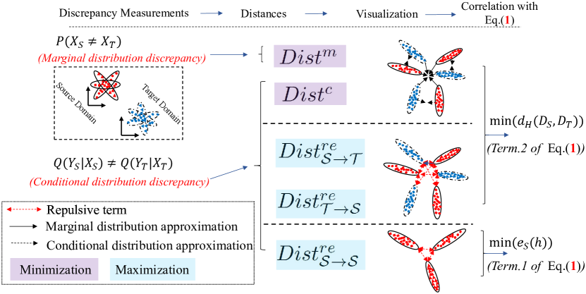
Figure 4: Purple parts represent distribution approximations across the source and target domains, w.r.t, marginal and conditional distribution divergence minimization. Blue parts denote discriminative distribution approximations across and within the source and target domains, respectively.

Matching Marginal and Conditional Distributions: As shown in Fig.4, our model starts from JDA [50], which makes use of MMD in RKHS to measure the distances between the expectations of the source domain/sub-domain and target domain/sub-domain. Specifically, 1) the empirical distance of the source and target domains is defined as $Dis{t^{m}}$; 2) the conditional distance $Dis{t^{c}}$ is defined as the sum of the empirical distances between pairs of sub-domains in ${{\cal D}_{\cal S}}$ and ${{\cal D}_{\cal T}}$ with the same label; 3) $Dis{t_{Clo}}$ is defined as the sum of $Dis{t^{m}}$ and $Dis{t^{c}}$, which will be optimized to bring closer both data distributions and class conditional data distributions across domains.

• $Dis{t^{m}}({{\cal D}_{\cal S}},{{\cal D}_{\cal T}})$: where ${{\bf{M}}_{0}}$ is the MMD matrix between ${{\cal D}_{\cal S}}$ and ${{\cal D}_{\cal T}}$ with ${{{({{\bf{M}}_{0}})}_{ij}}=\frac{1}{{{n_{s}}{n_{s}}}}}$ if $({{\bf{x}_{i}},{\bf{x}_{j}}\in{D_{S}}})$, ${{{({{\bf{M}}_{0}})}_{ij}}=\frac{1}{{{n_{t}}{n_{t}}}}}$ if $({{\bf{x}_{i}},{\bf{x}_{j}}\in{D_{T}}})$ and ${({{\bf{M}}_{0}})_{ij}}=\frac{{-1}}{{{n_{s}}{n_{t}}}}$ otherwise. Thus, the difference between the marginal distributions $\mathcal{P}(\mathcal{X_{S}})$ and $\mathcal{P}(\mathcal{X_{T}})$ is reduced when minimizing $Dis{t^{m}}({{\cal D}_{\cal S}},{{\cal D}_{\cal T}})$.

• $Dis{t^{c}}({{\cal D}_{\cal S}},{{\cal D}_{\cal T}})$: where $C$ is the number of classes, $\mathcal{D_{S}}^{(c)}=\{{\bf{x}_{i}}:{\bf{x}_{i}}\in\mathcal{D_{S}}\wedge y({\bf{x}_{i}})=c\}$ represents the ${c^{th}}$ sub-domain in the source domain, in which $n_{s}^{(c)}={\left\|{\mathcal{D_{S}}^{(c)}}\right\|_{0}}$ is the number of samples in the ${c^{th}}$ source sub-domain. $\mathcal{D_{T}}^{(c)}$ and $n_{t}^{(c)}$ are defined similarly for the target domain but using pseudo labels. Finally, $\bf M_{c}$ denotes the MMD matrix between the sub-domains with labels $c$ in ${{\cal D}_{\cal S}}$ and ${{\cal D}_{\cal T}}$ with ${{{({{\bf{M}}_{c}})}_{ij}}=\frac{1}{{n_{s}^{(c)}n_{s}^{(c)}}}}$ if $({{\bf{x}_{i}},{\bf{x}_{j}}\in{D_{S}}^{(c)}})$, ${{{({{\bf{M}}_{c}})}_{ij}}=\frac{1}{{n_{t}^{(c)}n_{t}^{(c)}}}}$ if $({{\bf{x}_{i}},{\bf{x}_{j}}\in{D_{T}}^{(c)}})$, ${{{({{\bf{M}}_{c}})}_{ij}}=\frac{{-1}}{{n_{s}^{(c)}n_{t}^{(c)}}}}$ if $({{\bf{x}_{i}}\in{D_{S}}^{(c)},{\bf{x}_{j}}\in{D_{T}}^{(c)}\;or\;\;{\bf{x}_{i}}\in{D_{T}}^{(c)},{\bf{x}_{j}}\in{D_{S}}^{(c)}})$ and ${{{({{\bf{M}}_{c}})}_{ij}}=0}$ otherwise. Consequently, the mismatch of conditional distributions between ${{D_{\cal S}}^{c}}$ and ${{D_{\cal T}}^{c}}$ is reduced by minimizing ${Dis{t^{c}}}$.

• Finally, the original data $\bm{X}$ are projected into the optimal common feature space using the mapping ${\bf{A}}$ through ${{\bf{A}}^{T}}{\bf{X}}$.

Repulsive Force (RF) Across/Within Domains: As shown in Fig.4, JDA is merely concerned with shrinking the MMD distances in order to reduce the cross-domain distribution divergence and ignores discriminative knowledge within data. Therefore, we directly borrow the idea from CDDA and DGA-DA [57, 55] and introduce the Repulsive Force(RF) term $Dis{t^{re}}{\text{ = }}Dist_{S\to T}^{re}+Dist_{T\to S}^{re}$ to further explore the discriminativeness of data. While JDA and DGA-DA have so far endeavored to minimize term.2 of Eq.(1), in this paper we additionally optimize term.1 of Eq.(1) as shown in Fig.4 and introduce a novel RF term $Dist_{{\cal S}\to{\cal S}}^{re}$ as in Fig.4, so as to increase the discriminative power of the labeled source domain data, thereby allowing a better predictive model on the source domain and a decreasing term.1 of Eq.(1). Subsequently, we use ${{\cal S}\to{\cal T}}$, ${{\cal T}\to{\cal S}}$ and ${{\cal S}\to{\cal S}}$ to index the distances computed from ${D_{\cal S}}$ to ${D_{\cal T}}$, ${D_{\cal T}}$ to ${D_{\cal S}}$ and ${D_{\cal S}}$ to ${D_{\cal S}}$, respectively, and $Dist_{{\cal S}\to{\cal T}}^{re}$ as the sum of the distances between each source sub-domain ${D_{\cal S}}^{(c)}$ and all the target sub-domains ${D_{\cal T}}^{(r);\;r\in\{\{1...C\}-\{c\}\}}$ excluding the $c$-th target sub-domain. Symmetrically, $Dist_{{\cal T}\to{\cal S}}^{re}$ and $Dist_{{\cal S}\to{\cal S}}^{re}$ are defined similarly to $Dist_{{\cal S}\to{\cal T}}^{re}$. Consequently, the final Repulsive Force term $Dis{t^{re}}$ is formalized as:

Where

• ${{\bf{M}}_{{\cal S}\to{\cal T}}}$ is defined as: ${{{({{\bf{M}}_{{\bf{S}}\to{\bf{T}}}})}_{ij}}=\frac{1}{{n_{s}^{(c)}n_{s}^{(c)}}}}$ if $({{\bf{x}_{i}},{\bf{x}_{j}}\in{D_{S}}^{(c)}})$, ${\frac{1}{{n_{t}^{(r)}n_{t}^{(r)}}}}$ if $({{\bf{x}_{i}},{\bf{x}_{j}}\in{D_{T}}^{(r)}})$, ${\frac{{-1}}{{n_{s}^{(c)}n_{t}^{(r)}}}}$ if $({{\bf{x}_{i}}\in{D_{S}}^{(c)},{\bf{x}_{j}}\in{D_{T}}^{(r)}\;or\;{\bf{x}_{i}}\in{D_{T}}^{(r)},{\bf{x}_{j}}\in{D_{S}}^{(c)}})$ and ${0}$ otherwise.

• ${{\bf{M}}_{{\cal T}\to{\cal S}}}$ is defined as: ${{{({{\bf{M}}_{{\bf{T}}\to{\bf{S}}}})}_{ij}}=\frac{1}{{n_{t}^{(c)}n_{t}^{(c)}}}}$ if ${({\bf{x}_{i}},{\bf{x}_{j}}\in{D_{T}}^{(c)})}$, ${\frac{1}{{n_{s}^{(r)}n_{s}^{(r)}}}}$ if ${({\bf{x}_{i}},{\bf{x}_{j}}\in{D_{S}}^{(r)})}$, ${\frac{{-1}}{{n_{t}^{(c)}n_{s}^{(r)}}}}$ if ${({\bf{x}_{i}}\in{D_{T}}^{(c)},{\bf{x}_{j}}\in{D_{S}}^{(r)}\;or\;{\bf{x}_{i}}\in{D_{S}}^{(r)},{\bf{x}_{j}}\in{D_{T}}^{(c)})}$ and ${0}$ otherwise.

• ${{\bf{M}}_{{\cal S}\to{\cal S}}}$ is defined as: ${{{({{\bf{M}}_{{\bf{S}}\to{\bf{S}}}})}_{ij}}=\frac{1}{{n_{s}^{(c)}n_{s}^{(c)}}}}$ if ${({x_{i}},{x_{j}}\in{D_{S}}^{(c)})}$, ${\frac{1}{{n_{s}^{(r)}n_{s}^{(r)}}}}$ if ${({x_{i}},{x_{j}}\in{D_{S}}^{(r)})}$, ${\frac{{-1}}{{n_{s}^{(c)}n_{s}^{(r)}}}}$ if ${({x_{i}}\in{D_{S}}^{(c)},{x_{j}}\in{D_{S}}^{(r)}\;or\;{x_{i}}\in{D_{S}}^{(r)},{x_{j}}\in{D_{S}}^{(c)})}$ and ${0}$ otherwise.

Therefore, maximizing $Dist_{{\cal S}\to{\cal T}}^{re}$ and $Dist_{{\cal T}\to{\cal S}}^{re}$ increases the distances of each sub-domain with the other remaining sub-domains across domains, i.e., the between-class distances across domains, thereby reducing term.2 of Eq.(1). On the other hand, maximizing $Dist_{{\cal S}\to{\cal S}}^{re}$ increases the between-class distances in the source domain, thereby optimizing term.1 in Eq.(1) on classification errors on the source domain. In our model, the RF term is proposed within the source domain and across the different domains simultaneously for optimizing the first and second terms of the right-hand in Eq.(1) simultaneously.

III-B2 Attention Regularized Laplace Graph

Although Sect.III-B1 improves CDDA and DGA-DA to optimize Term.1 and Term.2 of Eq.(1), minimization of Term.3 in Eq.(1) is not addressed and further requires manifold regularization in order to decrease the divergence between the classifiers on the source and target domains. However, as discussed in Sect.I, traditional manifold learning-based DA is not concerned with data class information and suffers from the so-called issue of ’Lack of Attention’. To remedy this issue, we introduce here an Attention Regularized Laplace Graph (ARG) term to explicitly address the issues of P1 and P2 as highlighted in Sect.I and to achieve discriminativeness aware manifold learning. Specifically, the proposed ARG aims to achieve the following two goals:

• Goal.1: To avoid the injudicious separation of data from the same sub-domain as shown in Fig.2.(b), the proposed ARG needs to bring closer those cross sub-domains with the same label but with large domain divergence.

• Goal.2: To prevent the brute force data geometric structure alignment as highlighted in Fig.2.(d), the designed ARG needs to enable separation of those differently labeled yet closely aligned sub-domains.

Mathematical Formalization: To meet Goal.1 and Goal.2, the ARG term is mathematically formalized through the following steps:

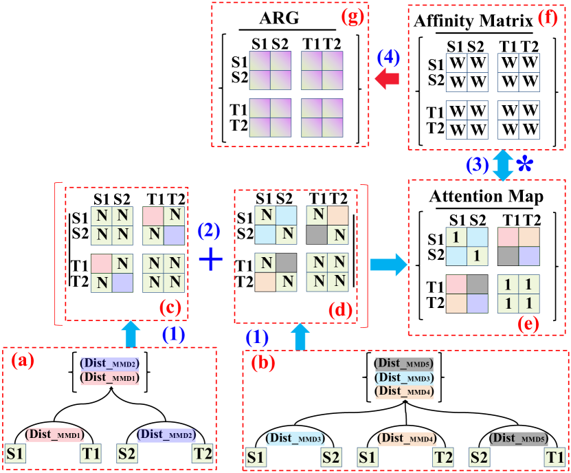
Figure 5: Detailed illustration of the proposed Attention Regularized Laplace Graph. Fig.5.(a,b). Cross sub-domain divergence; Fig.5.(c). Intra-Class Attraction Aware Attention Map; Fig.5.(d). Inter-Class Repulsion Aware Attention Map; Fig.5.(e). Attention Map; Fig.5.(g). Attention Regularized Laplace Graph.

• Step.1 - Design of an Affinity Matrix: Initially, an affinity matrix ${\bf{W}}$ is defined to capture the relative relationship of each sample across the whole database, which is also the fundamental framework of the ARG term. Formally, we denote the pair-wise affinity matrix as:

  where ${\bf{W}}={[{w_{ij}}]_{({n_{s}}+{n_{t}})\times({n_{s}}+{n_{t}})}}$ is a symmetric matrix [59], with ${w_{ij}}$ giving the affinity between two data samples $i$ and $j$ and defined as ${sim({x_{i}},{x_{j}})}=\exp(-\frac{{{{\left\|{{\bf{x}_{i}}-{\bf{x}_{j}}}\right\|}^{2}}}}{{2{\sigma^{2}}}})$ if $i\neq j$ and ${w_{ii}}=0$ otherwise. Similar to DGA-DA, the greater the distance between a pair of samples ${dist({x_{i}},{x_{j}})}$, the less their similarity ${sim({x_{i}},{x_{j}})}$, and vice versa.

• Step.2 - Computation of Cross Domain Intra-class Conditional Distribution Divergence: given the labels ranging from $1\to C$, leading to C pairs of sub-domains ${({D_{S}}^{c},{D_{T}}^{c})_{c\in(1...C)}}$ over the source and target domains, the cross domain intra sub-domain divergence is computed as $Dist_{c\in(1...C)}^{c}({D_{S}}^{c},{D_{T}}^{c})$, using the MMD measurement:

  Using Eq.(6), C cross sub-domain distances can be computed as illustrated in Fig.5.(a).

• Step.3 (Intra-Class Attraction Aware Attention Map): to meet Goal.1, we aim to decrease the dissimilarities of sub-domain pairs of the same label but with large distances, thereby bringing closer these cross sub-domains for class aware data geometric alignment. For this purpose, as illustrated in Fig.5.(c), we define the Intra-Class Attraction Aware Attention (A.Atten) as:

  By dot multiplication of Eq.(5) and Eq.(7), the affinity matrix receives an attention regularization, ${{\mathbf{W}}_{A.Atten}}{\text{ = }}{\mathbf{W}}\bullet A.Atten$, which amplifies the similarity of cross-domain data pairs when they belong to the same sub-domain.

• Step.4 (RF - Inter-class Conditional Distribution Divergence): We also calculate the conditional distribution divergence between differently labeled sub-domains in the source domain using MMD measurement.

  Similar to Eq.(6), Eq.(8) captures the distance between the differently labeled sub-domains in the source domain in terms of conditional distributions. Inspired by the Repulsive Force(RF) term as defined in Eq.(4), we name the distance of Eq.(8) as $RF.Dist$ to distinguish it from the class attraction distance in Eq.(6).

  As shown in Fig.5.(b), we also propose Eq.(9) to capture the distance between the differently labeled sub-domains across the source and target domains.

• Step.5 (Inter-Class Repulsion Aware Attention Map) To meet Goal.2, we need to decrease the similarities of closely confounded yet differently labeled sub-domain data. As shown in Fig.5.(d), Inter-Class Repulsion Aware Attention (R.Atten) is defined as:

  Using Eq.(10), the affinity matrix can be improved by attention regularization again, using the Inter-Class Repulsion Aware Attention Map (R.AM), through dot multiplication ${{\mathbf{W}}_{R.Atten}}{\text{ = }}{\mathbf{W}}\bullet R.Atten$, which decreases the affinities of sub-domain data that are differently labeled but very confounded in terms of data distributions.

• Step.6 (Attention Map): As shown in Fig.5.(c), by unifying the Intra-Class Attraction Attention Map A.AM and the Inter-Class Repulsion Attention Map R.AM, we obtain our final Attention Map (AM), where the empty position is embedded with ’1’ to preserve the original manifold structures.

• Step.7 (Attention Regularized Laplace Graph): Finally, the previous Attention Map is used to improve the traditional Laplace graph (${\mathbf{L}}$) in order to obtain the Attention Regularized Laplace Graph (ARG), which is mathematically formulated as:

  where ${{\mathbf{D}}_{AM}}=diag\{{d_{A{M_{11}}}}...{d_{A{M_{({n_{s}}+{n_{t}}),({n_{s}}+{n_{t}})}}}}\}$ is the degree matrix with ${d_{A{M_{ii}}}}=\sum\nolimits_{j}{{w_{A{M_{ij}}}}}$. The proposed ARG not only enables preservation of data manifold structures by following the standard spectral graph theory, but also modulates it by taking into account intra-class attraction and inter-class repulsion over the source and target domains, thereby leading to discriminative attention aware manifold embedding.

III-B3 FEEL-Based Manifold Alignment

to deal with the second issue (’Incomplete Unification’) as highlighted in Sect.I, we also propose a novel manifold learning strategy, which hybridizes the DGSA-GE-FE and DGSA-GE-LE approaches into a unified optimization framework and integrates seamlessly ARG-based embeddings, and formulate our final FEEL strategy for dynamic alignment of the manifold structures across different feature/label spaces as illustrated in Fig.6. Specifically, the proposed FEEL strategy aims to achieve the following three goals:

• Goal.3: Alignment of the manifold structures between the original feature space and the common feature space as enabled in the DGSA-GE-FE approach, thereby reducing term.3 of Eq.(1).

• Goal.4: Alignment of the common feature space and the label space as proposed in the DGSA-GE-LE techniques in order to decrease term.1 of Eq.(1).

• Goal.5: Seamless integration of the Attention Regularized Laplace Graph ARG for data distribution modulated graph-based embeddings.

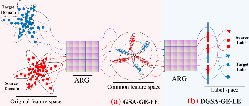
Figure 6: The proposed FEEL strategy is composed of DGSA-GE-FE and DGSA-GE-LE.

Implementation details: To meet Goal.3 through Goal.5, FEEL hybridizes (a). DGSA-GE-FE and (b). DGSA-GE-LE. Furthermore, inspired by DGA-DA [55], we also introduce the (c) Label Smoothness Consistency term (LSmC), to ensure robust functional learning.

(a). Feature Space Embedding: as shown in Fig.6.(a), FEEL starts by searching a common feature space $\mathcal{(C)}$ from the original feature space $\mathcal{(X)}$ using matrix transformation ($\mathop{\mathbf{X}}\limits_{\in\mathcal{X}}\to\mathop{{\mathbf{AX}}}\limits_{\in\mathcal{C}}$), while respecting the underlying data manifold geometric structure, and minimizes the following objective function:

where ${{\mathbf{W}}^{O}}$ denotes the affinity matrix which is based on the Original feature space, and ${{\mathbf{D}}^{O}}=diag\{d_{(1,1)}^{O}...d_{(({n_{s}}+{n_{t}}),({n_{s}}+{n_{t}}))}^{O}\}$ is the degree matrix with $d_{(i,i)}^{O}=\sum\nolimits_{j}{w_{(ij)}^{O}}$. Optimizing Eq.(12) merely deals with Goal.3. Therefore, we propose Eq.(13) to improve Eq.(12) via attention regularization to partially meet Goal.5.

Eq.(13) differs from Eq.(12) by reformulating ${{{\mathbf{W}}^{O}}}$ as ${{\mathbf{W}}_{AM}^{O}}$, thereby generating the attention aware DGSA-GE-FE.

(b). Label Space Embedding: as shown in Fig.6.(b), in order to meet Goal.4 and Goal.5, we further align the manifold structure across the common feature space $\mathcal{(C)}$ and the label space $\mathcal{(Y)}$ via ${\mathbf{AR}}{{\mathbf{G}}^{C}}$ regularized functional learning:

in which ${{\mathbf{W}}^{C}}$ is computed in the Common feature space.

(c). Label Smoothness Consistency: to enhance the robustness of dynamic functional learning across DGSA-GE-FE and DGSA-GE-LE, we borrow the merits of the label smoothness consistency (LSmC) term [28, 44] as proposed in DGA-DA:

$$\begin{array}[]{c}Dis{t^{lable}}=\sum\limits_{j=1}^{C}{\mathop{\sum}\limits_{i=1}^{{n_{s}}+{n_{t}}}}\left\|{\bf{Y}}^{(F)}_{i,j}-{\bf{Y}}^{(0)}_{i,j}\right\|\end{array}$$ (15)

in which ${\bf{Y}}={{\bf{Y}}_{\cal S}}\cup{{\bf{Y}}_{\cal T}}$, ${\bf{Y}}_{i,j}^{(F)}$ denotes the probability of ${i_{th}}$ data belonging to ${j_{th}}$ class, and each piece of data ${x_{i}}$ has a predicted label ${y_{i}}=\arg{\max_{j\leq c}}{\bf{Y}}_{ij}^{F}$. Indeed, the (LSmC) term is a constraint designed to prevent too many changes from the initial label assignment ${{\bf{Y}}_{\cal S}}$. By exploring the discriminative properties, we follow the experimental settings of DGA-DA and define the initial prediction ${{\bf{Y}}^{(0)}}$ as:

where $D_{\cal T}^{(c)}$ is defined as pseudo labels, generated via a base classifier, e.g., NN. Therefore, jointly optimizing Eq.(13), Eq.(14) and Eq.(15) ensures Goal.4 through Goal.5 and guarantees robust optimization simultaneously.

III-B4 The final model

To sum up, our final model (ARG-DA) jointly optimizes Eq.(3), Eq.(4), Eq.(13), Eq.(14), and Eq.(15) within a unified framework, which comprehensively minimizes the error bound as defined in Eq.(1) and simultaneously addresses the two issues highlighted in Sect.I, namely (’Lack of Attention’ and ’Incomplete Unification’). Specifically, it can be written mathematically as:

where ${{\mathbf{M}}^{*}}$ synthesizes the MMD matrices of both Eq.(3) and Eq.(4) to ensure a discriminative statistic alignment as discussed in Sect.III-B1. The constraint ${{{\bf{A}}^{T}}{\bf{XH}}{{\bf{X}}^{T}}{\bf{A}}={\bf{I}}}$ removes an arbitrary scaling factor in the embedding and prevents the above optimization from collapse onto a subspace of dimensions less than the required dimensions. On the other hand, $\lambda$ is a regularization parameter guaranteeing that the optimization problem is well-defined, and $\mu$ is a trade-off parameter which balances LSmC and label space embedding.

Fig.7 highlights the contribution of each component in Eq.(17) to decreasing the three terms of the error bound defined in Eq.(1):

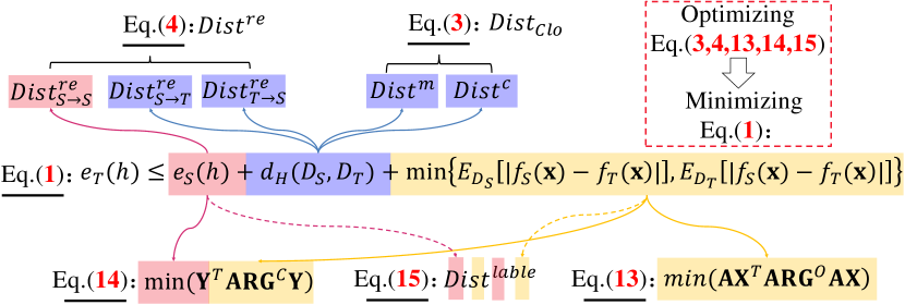
Figure 7: Highlight of Eq.(17) where the red, purple, and yellow parts denote the impact of various equations on Term.1, Term.2, and Term.3 in the error bound (Eq.(1)) limitation, respectively.

• Term.1: leveraging the labels available in the source domain, both Eq.(4) and Eq.(14) minimize Term.1 of Eq.(1) via distribution alignment and manifold regularization, respectively, while Eq.(15) enforces minimization of Term.1 through label propagation.

• Term.2: in line with the statistic alignment approach, joint optimization of $Dis{t^{m}}+Dis{t^{c}}$ in Eq.(3) and $Dist_{S\to T}^{re}+Dist_{T\to S}^{re}$ in Eq.(4) decreases the marginal and conditional distribution divergences, respectively, thereby enforcing minimization of Term.2 of Eq.(1);

• Term.3: optimizing Eq.(13) and Eq.(14) theoretically shrinks the divergence between different labeling functions, thereby reducing Term.3 of Eq.(1). Meanwhile, Eq.(15) partially shrinks Term.3 of Eq.(1) thanks to the joint optimization of Eq.(14) and Eq.(15).

III-C Solving the model

Optimization of our final model Eq.(17) is based on the following three key factors:

• F.1: Discriminative statistic alignment (Eq.(3), Eq.(4));

• F.2: ARG-based DGSA-GE-FE, which aligns the manifold structure across different feature spaces, (Eq.(13));

• F.3: ARG-based DGSA-GE-LE, which aligns the manifold structure across feature and label spaces, (Eq.(14), Eq.(15)).

These three key factors can be categorized into two sub-problems (SPs) for the dynamic functional learning:

• SP.1: in SP.1, both F.1 and F.2 enforce the domain alignment across the original feature space and the common feature space. Mathematically, SP.1 can be formalized as:

• SP.2: using the updated feature representation ${{{\mathbf{A}}^{T}}{\mathbf{X}}}$ of SP.1, SP.2 aligns the manifold structure across the common feature space and the label space to achieve F.3.

As a result, our final model Eq.(17) can thus be naturally divided into two sub-optimization problems (Eq.(18) and Eq.(19)), each of which has a closed form solution and can be optimized alternatively.

Optimization of SP.1: Eq.(18) amounts to solving the generalized eigendecomposition problem in order to obtain the best matrix projection $\bm{A}$. By using the Augmented Lagrangian method [15, 50], we obtain the best candidate matrix projection through setting its partial derivation w.r.t. $\bm{A}$ equal to zero:

where $\Phi{\rm{=diagram}}({\varphi_{1}},...{\varphi_{k}})\in{R^{k*k}}$ is the Lagrange multiplier, and ${\mathbf{AR}}{{\mathbf{G}}^{O}}$ is calculated using the original feature representation. The optimal subspace $\bm{A}$ is reduced to solving Eq.(20) for the k smallest eigenvectors. Then, we obtain the projection matrix $\bm{A}$ and the updated feature representation in the newly searched common feature space ${\bf{Z}}={{\bf{A}}^{T}}{\bf{X}}$.

Optimization of SP.2: using ${\bf{Z}}$ obtained in SP.1, we formulate ${\mathbf{AR}}{{\mathbf{G}}^{C}}$ to further explore the discriminative power of the label space ${\bf{Y}}$ by optimizing Eq.(19). Inspired by previous research [96] [35], the minimum of Eq.(19) is approached where the derivative of the function is zero. Therefore, the approximate solution can be formulated as:

where $\textbf{Y}^{\star}$ is the probability of prediction of the target domain corresponding to different class labels, ${\mathbf{W}}_{AM}^{C}$ is the affinity matrix based on the feature representation in the optimized common feature space, and ${\mathbf{D}}_{AM}^{C}$ is the diagonal matrix.

For simplicity’s sake, we define $\alpha{\rm{=}}\frac{1}{{1+\mu}}$, then Eq.(21) is reformulated as Eq.(22):

$${{\mathbf{Y}}^{\star}}={({\mathbf{D}}_{AM}^{C}-\alpha{\mathbf{W}}_{AM}^{C})^{-1}}{{\mathbf{Y}}^{(0)}}$$ (22)

To sum up, at a given iteration, SP.1 and SP.2 can be dynamically optimized to search the optimal solution and ensure the Attention Regularized Laplace Graph-based-DA.

The complete learning algorithm is summarized in Algorithm 1 - ARG-DA.

Input: Data $\bf{X}$, Source domain labels ${\bf{Y}}_{\cal S}$, subspace dimension $k$, number of iterations $T$, regularization parameters $\lambda$ and $\alpha$

1

2Step 1: Initialize the iteration counter t=0 and compute ${{\bf{M}}_{0}}$ as in Eq.(3).

3

4Step 2: Initialize pseudo target labels ${{\bf{Y}}_{\cal T}}$ and projection space A:

5

6Step 3: Initialize pseudo target labels ${{\bf{Y}}_{\cal T}}$ via a base classifier, e.g., 1-NN, based on source domain labels ${{\bf{Y}}_{\cal S}}$.

7Stage.1: while  Definition of Stage.1: do

8       (1) Initialize ${{\mathbf{AR}}{{\mathbf{G}}^{O}}}$ based on the pseudo target labels and the original feature representation $\bf{X}$ via Eq.(11).

9      (2) Solve the generalized eigendecomposition problem [15, 50] as in Eq.(20) (replace ${\mathbf{M}}^{*}$ by ${{\bf{M}}_{0}}$ ) and obtain adaptation matrix $\bf A$, then embed data via the transformation, $\bf{Z}={{\bf{A}}^{T}}{\bf{X}}$;

10      

11

12Stage.2: while  Definition of Stage.2: do

13       (1) Initialize ${{\mathbf{AR}}{{\mathbf{G}}^{O}}}$ based on the pseudo target labels and the common feature representation $\bf{Z}$ via Eq.(11).

14      (2) Solve the generalized eigendecomposition problem [15, 50] as in Eq.(20) (replace ${\mathbf{M}}^{*}$ by ${{\bf{M}}_{0}}$ ) and obtain adaptation matrix $\bf A$, then embed data via the transformation, $\bf{Z}={{\bf{A}}^{T}}{\bf{X}}$;

15      

16      (3) construct the label matrix ${{\bf{Y}}^{(0)}}$ as in Eq.(16), then obtain ${{\rm{{\bf{Y}}}}_{final}}$ by solving Eq.(21);

17      

18      (4) update pseudo target labels $\{{\bf{Y}}_{\cal T}^{(F)}={{\bf{Y}}_{final}}\left[{:,({n_{s}}+1):({n_{s}}+{n_{t}})}\right]\}$;

19      

20

21while not converged and $t<T$  do

22       Step 4: Update projection space A

23      

24      (i) Compute ${\bf{M}}_{c}$ as in Eq.(3)

25      (ii) Compute ${\mathbf{M}}^{*}$ as defined in Eq.(17) via updated ${{\bf{Y}}_{\cal T}}$.

26      Step 5: Stage.1:

27      Step 6: Stage.2:

28      Step 7: $t=t+1$; Return to Step 3;

29      

Output: Adaptation matrix ${\bf{A}}$, embedding ${\bf{Z}}$, Target domain labels ${\bf{Y}}_{\cal T}^{(F)}$

Algorithm 1 Attention Regularized Laplace Graph for Domain Adaptation (ARG-DA)

III-D Kernelization

The proposed ARG-DA method is extended to nonlinear problems in a Reproducing Kernel Hilbert Space via the kernel mapping $\phi:x\to\phi(x)$, or $\phi({\bf{X}}):[\phi({{\bf{x}}_{1}}),...,\phi({{\bf{x}}_{n}})]$, and the kernel matrix ${\bf{K}}=\phi{({\bf{X}})^{T}}\phi({\bf{X}})\in{R^{n*n}}$. We utilize the representer theorem to formulate the Kernel ARG-DA as:

IV Experiments

IV-A Benchmarks and Features

In this paper, as shown in Fig.8, we evaluate the proposed ARG-DA using standard benchmarks, i.e., USPS [30]+MINIST [37], COIL20 [50], PIE [50], office+Caltech [50], and SVHN-MNIST [4], and compare it with state-of-the-art DA methods. Following the experimental settings as reported in the previous works [17, 10, 56, 4, 45], we construct 37 datasets for different image classification tasks.

Office+Caltech consists of 2533 images of 10 categories (8 to 151 images per category per domain) [17]. These images come from four domains: (A) AMAZON, (D) DSLR, (W) WEBCAM, and (C) CALTECH. AMAZON images were acquired in a controlled environment with studio lighting. DSLR consists of high-resolution images captured by a digital SLR camera in a home environment under natural lighting. WEBCAM images were acquired in a similar environment to DSLR but with a low-resolution webcam. CALTECH images were collected from Google Images.

We use two types of image features extracted from these datasets, i.e., SURF and DeCAF6, which are publicly available. The SURF [18] features are shallow features extracted and quantized into an 800-bin histogram using a codebook computed with K-means on a subset of images from Amazon. The resultant histograms are further standardized by z-score. The Deep Convolutional Activation Features (DeCAF6) [13] are deep features computed as in AELM [80], which makes use of the VLFeat MatConvNet library with different pretrained CNN models, including in particular the Caffe implementation of AlexNet [36] trained on the ImageNet dataset. The outputs from the 6th layer are used as deep features, leading to 4096 dimensional DeCAF6 features. In this experiment, we denote the dataset Amazon, Webcam, DSLR, and Caltech-256 as A, W, D, and C, respectively. The arrow ”$\rightarrow$” is proposed to denote the direction from ”source” to ”target”. For example, ”W $\rightarrow$ D” means the Webcam image dataset is considered as the labeled source domain, whereas the DSLR image dataset is the unlabeled target domain.

USPS+MNIST shares 10 common digit categories from two subsets, namely USPS and MNIST, which have very different data distributions (see Fig.8). We construct a first DA task USPS vs MNIST by randomly sampling the first 1,800 images in USPS to form the source data, followed by 2,000 images in MNIST to form the target data. Then, we switch the source/target pair to get another DA task, i.e., MNIST vs USPS. We uniformly rescale all images to size $16\times 16$ and represent each one by a feature vector encoding the gray-scale pixel values. We also extract deep features from the softmax layer [67] of the LeNet [37] architecture, leading to a 10-dimensional feature. Thus, the source and target domain data share the same feature space. As a result, we have defined two cross-domain DA tasks, namely USPS $\rightarrow$ MNIST and MNIST $\rightarrow$ USPS.

COIL20 contains 20 objects with 1,440 images (Fig.8). The images of each object were taken by varying its pose by about 5 degrees, resulting in 72 poses per object. Each image has a resolution of 32*32 pixels and 256 gray levels per pixel. In this experiment, we partition the dataset into two subsets, namely COIL 1 and COIL 2 [88]. COIL 1 contains all images taken within the directions in $[{0^{0}},{85^{0}}]\cup[{180^{0}},{265^{0}}]$ (quadrants 1 and 3), resulting in 720 images. COIL 2 contains all images taken in the directions within $[{90^{0}},{175^{0}}]\cup[{270^{0}},{355^{0}}]$ (quadrants 2 and 4) and thus the number of images is also 720. In this way, we construct two subsets with relatively different distributions. In this experiment, the COIL20 dataset with 20 classes is split into two DA tasks, i.e., COIL1 $\rightarrow$ COIL2 and COIL2 $\rightarrow$ COIL1.

The PIE face database consists of 68 subjects, each under 21 various illumination conditions [10, 50]. We adopt five pose subsets: C05, C07, C09, C27, C29, which provide a rich basis for domain adaptation, that is, we can choose one pose as the source and any remaining one as the target. Therefore, we obtain $5\times 4=20$ different source/target combinations. Finally, we combine all five poses to form a single dataset for a large-scale transfer learning experiment. We crop all images to $32\times 32$ and only adopt the pixel values as the input. We denote the five subsets with different face poses as PIE1, PIE2, etc., and generate $5\times 4=20$ DA tasks, i.e., PIE1 vs PIE 2 $\dots$ PIE5 vs PIE 4, respectively.

SVHN-MNIST contains the MNIST dataset as introduced in USPS-MNIST but also the Street View House Numbers (SVHN), which is a collection of house numbers collected from Google street view images (see Fig.8). SVHN is quite distinct from the dataset of handwriting digits, i.e., digits in MNIST. Moreover, both domains are quite large, each having at least 60k samples over 10 classes. We propose to make use of the LeNet architecture [37] and domain classifier as introduced in [67] to extract features for our DA tasks.

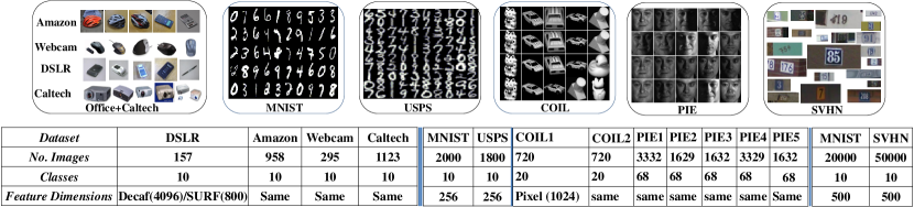
Figure 8: Sample images from seven datasets used in our experiments. Each dataset represents a different domain. The Office dataset in Office+Caltech contains three sub-datasets, namely DSLR, Amazon, and Webcam.

IV-B Baseline Methods

The proposed ARG-DA method is compared with thirty-three methods from the literature, which can be differentiated according to whether they are built on the deep learning-based framework:

• Shallow methods: (1) 1-Nearest Neighbor Classifier(NN); (2) Principal Component Analysis (PCA); (3) GFK [18]; (4) TCA [60]; (5) TSL [73]; (6) JDA [50]; (7) ELM [80]; (8) AELM [80]; (9) SA [14]; (10) mSDA [5]; (11) TJM [51]; (12) RTML [10]; (13) SCA [17]; (14) CDML [83]; (15) LTSL [72]; (16) LRSR [88]; (17) KPCA [69]; (18) JGSA [91]; (19) CORAL [75]; (20) RVDLR [31]; (21) LPJT [39]; (22) DGA-DA [55]; (23) GEF through its different variants, GEF-PCA,GEF-LDA, GEF-LMNN, and GEF-MFA [6].

• Deep methods: (24) AlexNet [36]; (25) DAH [82]; (26) DANN [16]; (27) ADDA [78]; (28) LTRU) [70]; (29) ATU [68]; (30) BSWD [67]; (31) DSN [4]; (32) DDC [79]; (33) DAN [48].

A direct comparison of the proposed ARG-DA using shallow features against DL-based DA methods could be unfair. To address this issue, in this paper, following the previous experimental settings as reported in DGA-DA, JGSA and BSWD, we make use of a deep feature, namely DeCAF6, as the input feature for a fair comparison with the DL-based DA methods. Whenever possible, the reported performance scores of the thirty-three methods from the literature are directly collected from their original papers or previous research [78, 80, 39, 17, 67, 91, 55, 6]. They are assumed to be their best performance.

IV-C Experimental Setup

Given the fact that the target domain has no labeled data under the experimental setting of UDA, it is not possible to tune a set of optimal hyper-parameters. In this paper, following the setting of previous research [55, 50, 88], we also evaluate the proposed ARG-DA by empirically searching the parameter space for the optimal settings. Specifically, the proposed ARG-DA method has three hyper-parameters, i.e., the subspace dimension $k$, and regularization parameters $\lambda$ and $\alpha$. In our experiments, we set $k=200$ and 1) $\lambda=0.1$, and $\alpha=0.9$ for USPS, MNIST, COIL20, and PIE, 2) $\lambda=1$, $\alpha=0.9$ for Office+Caltech, and SVHN-MNIST.

In our experiment, accuracy on the test dataset as defined by Eq.(24) is used as the performance measurement. It is widely applied in a series of previous research work, e.g., [48, 56, 50, 88], etc.

$$\begin{array}[]{c}Accuracy=\frac{{\left|{x:x\in{D_{T}}\wedge\hat{y}(x)=y(x)}\right|}}{{\left|{x:x\in{D_{T}}}\right|}}\end{array}$$ (24)

where ${\cal{D_{T}}}$ is the target domain treated as test data, ${\hat{y}(x)}$ is the predicted label, and ${y(x)}$ is the ground truth label for the test data $x$.

As discussed in Sect.III-B, the core model of the proposed ARG-DA method is originated from DGA-DA but combines two optimization strategies, namely the Attention Regularized Laplace Graph (ARG) term as defined in Eq.(11), and the Joint Manifold Alignment Strategy (’FEEL’) as introduced in Sect.III-B3. To gain insight into the proposed ARG-DA and the rationale w.r.t the ARG term and the FEEL strategy, we derive from Eq.(17) one intermediate partial model, namely DGA+A, to highlight the contribution of each optimization strategy to the final proposed ARG-DA:

• DGA+A: in this setting, we remove ${{\mathbf{AR}}{{\mathbf{G}}^{O}}}$ from Eq.(17) and derive the DGA+A model, which only makes use of the ARG mechanism as defined in Eq.(11) but without the ’FEEL’ strategy as defined in Sect.III-B3. This setting makes it possible to understand the contribution of the proposed ARG mechanism when the different sub-domain adaptation is properly regularized to remedy one of the raised issues, namely ’Lack of Attention’, by comparing it with its baseline DA model DGA-DA. Specifically, the mathematical formulations of both DGA+A and DGA-DA are depicted in Fig.18 for better clarity.

• ARG-DA: now our proposed ARG-DA improves DGA+A by further implementing the ’FEEL’ strategy to additionally align the original feature manifold for comprehensive manifold unification. With ARG+A as baseline, it is now possible to highlight the contribution of the ’FEEL’ strategy when all the manifold structures are further aligned.

IV-D Experimental Results and Discussion

IV-D1 Experiments on the CMU PIE Data Set

The CMU PIE database is a large face dataset containing 68 people with different pose, illumination, and expression variations. Fig.9 synthesizes the experimental results for DA using this dataset, where the best results are highlighted in red. The following observations can be drawn from Fig.9:

• by implementing the Attention Regularized Laplace Graph Enforced Adaptation model, DGA+A enhances discriminativeness across different sub-domains, thereby improving its baseline DGA-DA by 16 points, and achieves $81.25\%$ accuracy. By making use of the FEEL strategy, ARG-DA additionally improves DGA+A by roughly 1 point and highlights the interest of unifying the alignment of different feature/label manifolds.

• Interestingly, the second best performing methods are GEF-PCA and GEF-LDA, respectively. They are both variants of GEF [6]. GEF-PCA, formalized as Eq.(25), improves the baseline JDA by 15 points by incorporating a specifically designed revision graph ${\Delta{\mathbf{G}}}$ in order to increase within-class compactness.

• On the other hand, GEF-LDA draws inspiration from Linear Discriminant Analysis (LDA) [58], and replaces the constraint ${{{\mathbf{A}}^{T}}{\mathbf{XH}}{{\mathbf{X}}^{T}}{\mathbf{A}}={\mathbf{I}}}$ in GEF-PCA by ${{{\mathbf{A}}^{T}}{\mathbf{XP}}{{\mathbf{X}}^{T}}{\mathbf{A}}={\mathbf{I}}}$. Also, it further leverages the supervised knowledge embedded in the graph matrix $\mathbf{P}$ in order to minimize within-class scatter and maximize inter-class scatter, thereby further improving GEF-PCA by 1 point.

• The proposed ARG-DA is different from GEF-LDA. ARG-DA explicitly enhances inter-class discriminativeness through the designed repulsive force term as in Eq.(4), while the effectiveness of within-class compactness as highlighted in GEF-PCA is potentially enforced by dynamically regressing the common feature representation to the discriminative label space through the proposed ARG term (Sect.III-B2) regularized DGA+A. Finally, ARG-DA improves DGA+A by additionally enabling the smooth manifold alignment across different feature spaces and thus achieves the best accuracy of $81.18\%$.

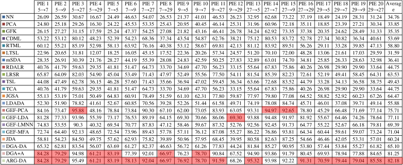
Figure 9: Accuracy${\rm{\%}}$ on the PIE Images Dataset.

IV-D2 Experiments on the USPS+MNIST Dataset

Figure 10: Accuracy${\rm{\%}}$ on the USPS+MNIST Image Dataset.

The USPS+MNIST dataset displays different writing styles between the source and target domains. In Fig.10, the left-hand columns of the red vertical bar report the experimental results using shallow features, whereas the right-hand columns of the red bar display the results of the methods using deep features.

• Using shallow features, DGA-DA outperforms both GEF-PCA and GEF-LDA by a large margin on the USPS+MNIST dataset. This is in contrast with the previous results in Sect.IV-D1 where GEF-PCA and GEF-LDA achieve higher accuracy than DGA-DA. We suspect that the main reason is due to the random writing styles of the USPS+MNIST dataset, which generates a more sophisticated data manifold structure than the one by predefined pose variations of the PIE dataset. As a result, by explicitly capturing the underlying geometric structures through the Laplace graph and leveraging manifold learning (${{\mathbf{Y}}^{T}}{\mathbf{LY}}$), as well as the label smoothness consistency (Eq.(15)) for robust label propagation, DGA-DA seems better armed to solve the complex manifold structure induced by DA tasks.

• By re-weighting the corresponding distances across different sub-domains for intra-class and inter-class aware DA, DGA+A improves DGA-DA by 1 point and achieves $77.70\%$ accuracy. By taking advantage of the ’FELL’ strategy for comprehensive manifold learning, ARG-DA further improves DGA+A and achieves $79.94\%$ accuracy.

• In the right-hand part of the red vertical bar in Fig.10, we also compare our approach with deep network-based methods, i.e., ADDA and DANN, which search a common latent subspace by shrinking the domain divergence using the adversarial learning strategy, and improve the performance of traditional DA methods by a large margin. Using deep features [67], ARG-DA demonstrates its effectiveness and outperforms deep learning-based DA methods, e.g., ADDA and DANN, by a margin of 16 and 2 points, respectively.

IV-D3 Experiments on the Office+Caltech-256 Datasets

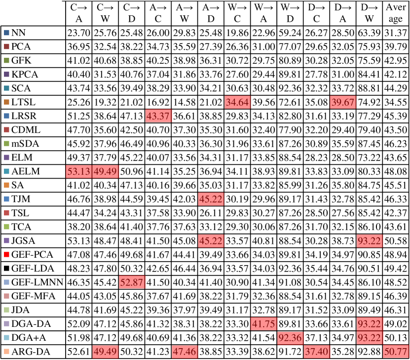
Figure 11: Accuracy${\rm{\%}}$ on the Office+Caltech Images with SURF-BoW Features.

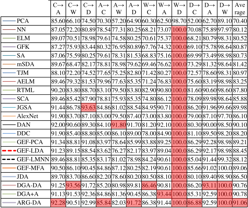
Figure 12: Accuracy${\rm{\%}}$ on the Office+Caltech Images with DeCAF6 Features.

Fig.11 and Fig.12 synthesize the experimental results in comparison with the state-of-the-art when classic shallow features (i.e., SURF features) and deep features (i.e., DeCAF6 features) are used, respectively. From Fig.11 and Fig.12, the following observations can be drawn:

• In both Fig.11 and Fig.12, DGA+A outperforms DGA-DA, which suggests the effectiveness of ARG enforced attention aware DA w.r.t. different feature representations. Meanwhile, it can be observed that ARG-DA improves DGA+A in both Fig.11 and Fig.12, thereby further demonstrating the contribution of the ’FEEL’ strategy to comprehensive manifold learning.

• In Fig.12 using deep features, both DGA+A and ARG-DA improve their performance as reported in Fig.11 by a very large margin. These results demonstrate that deep features can be seamlessly embedded into the proposed DA models for improved performance.

IV-D4 Large-Scale Experiments on the SVHN-MNIST Dataset

Different from the other datasets, SVHN-MNIST is composed of 50k and 20k real-world images from two very different domains, respectively, thereby generating a large-scale DA benchmark. Following the same experimental setting of previous research [55], Fig.13 reports the final experimental results. As shown in Fig.13, thanks to the effectiveness of the ARG term enforced manifold embeddings, DGA+A improves DGA-DA by 1 point. Furthermore, by additionally embracing the FEEL strategy ensured comprehensive manifold learning techniques, ARG-DA further improves DGA+AA by an accuracy of 1 point. In Fig.13, ARG-DA achieves the best performance, even in comparison with a series of state-of-the-art deep learning-based DA methods, thereby further demonstrating its effectiveness.

Figure 13: Accuracy${\rm{\%}}$ on the SVHN-MNIST Images Dataset.

IV-D5 Experiments on the COIL 20 Dataset

The COIL dataset (see fig.8) features the challenge of pose variations between the source and target domains. Even though DGA-DA already achieves $100.00\%$ accuracy on the COIL dataset, we still benchmark our proposed ARG-DA in order to see how the proposed ARG term and FEEL strategy impact the best baseline performance. Fortunately, both DGA+A and ARG-DA achieve $100.00\%$ accuracy and verify the robustness of the proposed ARG term and FEEL strategy.

IV-E Empirical Analysis

Although the proposed ARG-DA achieves state-of-the-art performance over 37 DA tasks through 7 datasets, an interesting question is how fast the proposed method converges (sect.IV-E2), as well as its sensitivity w.r.t. its hyper-parameters (Sect.IV-E1). Additionally, in Sect.IV-E3, we also aim to explore the robustness of the proposed FEEL strategy (Sect.III-B3) without the collaboration of the ARG term.

IV-E1 Sensitivity of the proposed ARG-DA w.r.t. hyper-parameters

Three hyper-parameters, namely $k$, $\lambda$ and $\alpha$, are used in the proposed DA method.

• $k$ denotes the dimension of the searched shared latent feature subspace, which determines the structure of low-dimension embedding. Obviously, the larger $k$, the more the shared subspace can afford complex data distributions, but at the cost of increased computation complexity.

• $\lambda$ defined in Eq.(23) aims to regularize the projection matrix $A$ to avoid over-fitting the chosen shared feature subspace w.r.t. both the source and the target domain. Increasing $\lambda$ reduces the risk of model over-fitting but shrinks the diversity of the functional learning representations.

• $\alpha{\rm{=}}\frac{1}{{1+\mu}}$ as defined in Eq.(23) is a trade-off parameter, which balances LSmC term (Eq.(15)) and label space embedding (Eq.(14)). Thus, increasing $\alpha$ improves the effectiveness of label space embedding, while reducing the contribution of label smoothness regularization.

Sensitivity of $k$: in Fig.16, we plot the classification accuracies of the proposed DA method w.r.t different values of $k$ on the PIE dataset. As shown in Fig.16, the subspace dimensionality $k$ varies with $k\in\{20,40,60,80,100,150,200,300,400\}$. The proposed two DA variants, namely, DGA+A and ARG-DA, remain stable w.r.t. a wide range of $k\in\{60\leq k\leq 400\}$. Finally, in this paper, we set $k=200$ to balance efficiency and accuracy.

Sensitivity of $\lambda$ and $\alpha$: we also study the sensitivity of the proposed DGA+A and ARG-DA methods with a wide range of hyper-parameter values, i.e., $\alpha=(0.01,0.05,0.1,0.5,0.9,0.95,0.99)$ and $\lambda=(0.001,0.002,0.005,0.1,1,5,10)$. We plot in Fig.17 the results on COIL1 $\rightarrow$ COIL2 $and$ MNIST $\rightarrow$ USPS datasets on both methods with $k$ held fixed at $200$. As shown in Fig.17, the proposed DGA+A and ARG-DA display their stability as the resultant classification accuracy remains roughly the same despite a wide range of $\lambda$ and $\alpha$ values, thereby suggesting that the proposed methods can easily search the proper candidate for these hyper-parameters.

IV-E2 Convergence analysis

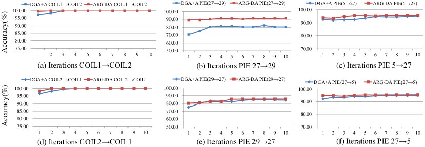
Figure 14: Convergence analysis using 6 cross-domain image classification tasks on COIL and PIE datasets. (accuracy w.r.t $\#$iterations)

Another interesting question is to see when the proposed methods achieve their best performance w.r.t. the number of iterations $T$. For this purpose, in Fig.14, we carry out a convergence analysis of the proposed DGA+A and ARG-DA models, using the pixel value features on both the PIE and COIL datasets. Subsequently, Fig.14 reports 6 cross DA experiments ( COIL1 $\rightarrow$ 2, COIL2 $\rightarrow$ COIL1 … PIE-27 $\rightarrow$ PIE-5 ) with the number of iterations $T=(1,2,3,4,5,6,7,8,9,10)$. As can be seen in Fig.14, both DGA+A and ARG-DA converge within 3$\sim$5 iterations when performing optimization over the two datasets. On the other hand, ARG-DA requires slightly more computational time per iteration than DGA+A, due to the computation of the additionally designed ${{\mathbf{AR}}{{\mathbf{G}}^{O}}}$, which discriminatively aligns different feature spaces. However, thanks to the FEEL strategy, the convergence curve displayed by ARG-DA is flatter in comparison with DGA+A.

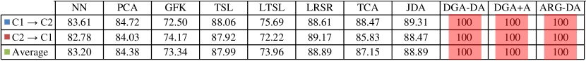
Figure 15: Accuracy${\rm{\%}}$ on the COIL Images Dataset.

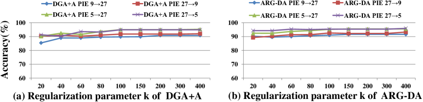
Figure 16: Sensitivity analysis of the proposed methods using the PIE dataset: (a) accuracy w.r.t. subspace dimension $k$ of DGA+A; (b) accuracy w.r.t. subspace dimension $k$ of ARG-DA.

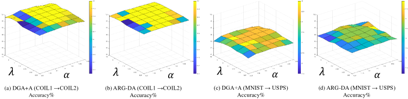
Figure 17: The classification accuracies of the proposed ARG-DA and DGA+A methods vs.the parameters $\alpha$ and $\lambda$ on the selected three cross-domain datasets.

IV-E3 Robustness of the FEEL-based comprehensive manifold learning

The FEEL strategy proposed in the ARG-DA model consists in aligning the manifold structures (MS) across the following groups of feature/label spaces:

• (G1). manifold structure across the original feature space (${\mathcal{X}}$) and the optimized common feature space (${\mathbf{A}}*{\mathcal{X}}$);

• (G2). manifold structure across the optimized feature space (${\mathbf{A}}*{\mathcal{X}}$) and the label space (${\mathcal{Y}}$);

Alignment of G1 or G2 in DA has already shown their effectiveness in a series of current research work, thereby encouraging hybridization of the previous two approaches by aligning jointly G1 and G2 within a unified optimization framework, as is the case in the proposed FEEL strategy. Even though the contribution of the FEEL strategy has already been highlighted by contrasting ARG-DA with its baseline model, DGA+A, over various datasets, we are still curious about the effectiveness of the FEEL strategy when it is disentangled from ARG regularization as in our previously proposed DGA-DA model. For this purpose, we derive a novel partial model, namely, DGA+F, which is formulated in Eq.(26)

Where ${{\mathbf{L^{\prime}}}}$ and ${\mathbf{L}}$ intend to align the manifold structures of G1 and G2, respectively. To gain insight into the proposed FEEL strategy, we draw the general optimization framework in Fig.18, where four different experimental settings, e.g., DGA-DA, DGA+F, DGA+A, and ARG-DA, are clearly distinguished by varying Term.1 and Term.2 of the optimization framework.

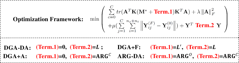
Figure 18: Detailed discussion of the differences across the DGA-DA, DGA+F, DGA+A, and ARG-DA algorithms.

Fig.19 shows the performance of the four experimental settings using the pixel value features on both the USPS+MNIST and COIL datasets. As shown in Fig.19, the following can be observed:

• Mathematically, DGA+F is different from DGA-DA by updating Term.1 as ${\mathbf{L^{\prime}}}$, which intends to additionally align the manifold structure across G1. However, DGA+F underperforms in comparison with its baseline, DGA-DA, both on the USPS+MNIST and COIL datasets.

• Under the condition of using the ARG term-based regularization, ARG-DA improves DGA+A by incorporating the FEEL strategy, which can be seen on both the USPS+MNIST and COIL datasets, in line with the results analyzed in Sect.IV-D1 through Sect.IV-D4.

To conclude, the FEEL strategy cannot be simply incorporated into the DGA-DA model. Due to the manifold structure divergence caused by domain shift , brutally aligning the manifold structure across G1 hurts the final DA performance. In this paper, by collaborating with the ARG term, the FEEL strategy is seamlessly embedded into the DGA+A model to dynamically align the manifold structure across different feature/label spaces and eventually achieve comprehensive manifold learning.

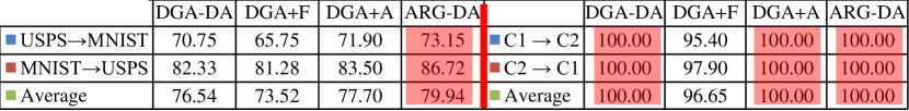
Figure 19: Accuracy${\rm{\%}}$ on the USPS+MNIST Images Dataset using different experimental settings.

V Conclusion

In this paper, we proposed a novel unsupervised DA method, namely Attention Regularized Laplace Graph-based Domain Adaptation (ARG-DA), which provides new perspectives, i.e., class aware attention and manifold alignment, to further explore Laplace graph-based DA methods. By weighting the importance of different sub-domain adaptations, we designed the Attention Regularized Laplace Graph to enforce the attention aware DA model DGA+A. Moreover, by unifying knowledge across different feature/label spaces, we improved DGA+A by incorporating the FEEL strategy for comprehensive manifold learning, thereby providing our final ARG-DA. Comprehensive experiments using the standard benchmark in DA showed the effectiveness of the proposed method, which consistently outperforms state-of-the-art DA methods. Future work includes embedding of the proposed ARG-DA into the paradigm of deep learning in order to improve the real computer vision applications, e.g., detection, segmentation, and tracking, etc.

Lingkun Luo was awarded his Ph.D degree at the Shanghai Jiao Tong University. He served as research assistant and postdoc in the Ecole Centrale de Lyon, Department of Mathematics and Computer Science, and was a member of the LIRIS laboratory. Today, he is a research fellow of the Shanghai Jiao Tong University. He has authored more than 20 research papers. His research interests include machine learning, pattern recognition, and computer vision.

Liming Chen was awarded a joint B.Sc. degree in mathematics and computer science from the University of Nantes, Nantes, France in 1984, as well as M.Sc. and Ph.D. degrees in computer science from the University of Paris 6, Paris, France, in 1986 and 1989, respectively. He first served as an Associate Professor with the Université de Technologie de Compiègne, before joining the École Centrale de Lyon, Écully, France, as a Professor in 1998, where he leads an advanced research team on Computer Vision, Machine Learning, and Multimedia. From 2001 to 2003, he also served as Chief Scientific Officer in a Paris-based company, Avivias, specializing in media asset management. In 2005, he served as Scientific Multimedia Expert for France Telecom R&D China, Beijing, China. He was the Head of the Department of Mathematics and Computer Science in the École Centrale de Lyon from 2007 through 2016. His current research interests include computer vision, machine learning, image and multimedia, with a particular focus on robot vision and learning since 2016. Liming has authored over 300 publications and has successfully supervised more than 40 Ph.D students. He has been a grant holder for a number of research grants from the EU FP program, French research funding bodies, and local government departments. Liming has so far guest-edited 5 journal special issues. He is an associate editor for the Eurasip Journal on Image and Video Processing and a senior IEEE member.

Shiqiang Hu was awarded his Ph.D degree at the Beijing Institute of Technology. He has authored over 150 publications and has successfully supervised more than 15 Ph.D students. Today, he is a full professor at the Shanghai Jiao Tong University. His research interests include data fusion technology, image understanding, and nonlinear filter.

References

- [1] Mikhail Belkin and Partha Niyogi. Laplacian eigenmaps for dimensionality reduction and data representation. Neural computation, 15(6):1373–1396, 2003.
- [2] Shai Ben-David, John Blitzer, Koby Crammer, Alex Kulesza, Fernando Pereira, and Jennifer Wortman Vaughan. A theory of learning from different domains. Machine learning, 79(1):151–175, 2010.
- [3] Karsten M Borgwardt, Arthur Gretton, Malte J Rasch, Hans-Peter Kriegel, Bernhard Schölkopf, and Alex J Smola. Integrating structured biological data by kernel maximum mean discrepancy. Bioinformatics, 22(14):e49–e57, 2006.
- [4] Konstantinos Bousmalis, George Trigeorgis, Nathan Silberman, Dilip Krishnan, and Dumitru Erhan. Domain separation networks. In Advances in Neural Information Processing Systems, pages 343–351, 2016.
- [5] Minmin Chen, Zhixiang Eddie Xu, Kilian Q. Weinberger, and Fei Sha. Marginalized denoising autoencoders for domain adaptation. CoRR, abs/1206.4683, 2012.
- [6] Yiming Chen, Shiji Song, Shuang Li, and Cheng Wu. A graph embedding framework for maximum mean discrepancy-based domain adaptation algorithms. IEEE Trans. Image Process., 29:199–213, 2020.
- [7] Nicolas Courty, Rémi Flamary, Amaury Habrard, and Alain Rakotomamonjy. Joint distribution optimal transportation for domain adaptation. In Advances in Neural Information Processing Systems, pages 3733–3742, 2017.
- [8] Nicolas Courty, Rémi Flamary, Devis Tuia, and Alain Rakotomamonjy. Optimal transport for domain adaptation. IEEE transactions on pattern analysis and machine intelligence, 39(9):1853–1865, 2017.
- [9] Debasmit Das and CS George Lee. Unsupervised domain adaptation using regularized hyper-graph matching. In 2018 25th IEEE International Conference on Image Processing (ICIP), pages 3758–3762. IEEE, 2018.
- [10] Zhengming Ding and Yun Fu. Robust transfer metric learning for image classification. IEEE Trans. Image Processing, 26(2):660–670, 2017.
- [11] Zhengming Ding and Yun Fu. Robust multiview data analysis through collective low-rank subspace. IEEE Trans. Neural Netw. Learning Syst., 29(5):1986–1997, 2018.
- [12] Jeff Donahue, Judy Hoffman, Erik Rodner, Kate Saenko, and Trevor Darrell. Semi-supervised domain adaptation with instance constraints. In Proceedings of the IEEE conference on computer vision and pattern recognition, pages 668–675, 2013.
- [13] Jeff Donahue, Yangqing Jia, Oriol Vinyals, Judy Hoffman, Ning Zhang, Eric Tzeng, and Trevor Darrell. Decaf: A deep convolutional activation feature for generic visual recognition. In Proceedings of the 31th International Conference on Machine Learning, ICML 2014, Beijing, China, 21-26 June 2014, pages 647–655, 2014.
- [14] Basura Fernando, Amaury Habrard, Marc Sebban, and Tinne Tuytelaars. Unsupervised visual domain adaptation using subspace alignment. In IEEE International Conference on Computer Vision, ICCV 2013, Sydney, Australia, December 1-8, 2013, pages 2960–2967, 2013.
- [15] Michel Fortin and Roland Glowinski. Augmented Lagrangian methods: applications to the numerical solution of boundary-value problems, volume 15. Elsevier, 2000.
- [16] Yaroslav Ganin, Evgeniya Ustinova, Hana Ajakan, Pascal Germain, Hugo Larochelle, François Laviolette, Mario Marchand, and Victor Lempitsky. Domain-adversarial training of neural networks. The Journal of Machine Learning Research, 17(1):2096–2030, 2016.
- [17] Muhammad Ghifary, David Balduzzi, W. Bastiaan Kleijn, and Mengjie Zhang. Scatter component analysis: A unified framework for domain adaptation and domain generalization. IEEE Trans. Pattern Anal. Mach. Intell., 39(7):1414–1430, 2017.
- [18] Boqing Gong, Yuan Shi, Fei Sha, and Kristen Grauman. Geodesic flow kernel for unsupervised domain adaptation. In Computer Vision and Pattern Recognition (CVPR), 2012 IEEE Conference on, pages 2066–2073. IEEE, 2012.
- [19] Rui Gong, Wen Li, Yuhua Chen, and Luc Van Gool. DLOW: domain flow for adaptation and generalization. In IEEE Conference on Computer Vision and Pattern Recognition, CVPR 2019, Long Beach, CA, USA, June 16-20, 2019, pages 2477–2486. Computer Vision Foundation / IEEE, 2019.
- [20] Ian Goodfellow, Yoshua Bengio, and Aaron Courville. Deep learning. MIT press, 2016.
- [21] Ian Goodfellow, Jean Pouget-Abadie, Mehdi Mirza, Bing Xu, David Warde-Farley, Sherjil Ozair, Aaron Courville, and Yoshua Bengio. Generative adversarial nets. In Advances in neural information processing systems, pages 2672–2680, 2014.
- [22] Arthur Gretton, Karsten M Borgwardt, Malte Rasch, Bernhard Schölkopf, and Alex J Smola. A kernel method for the two-sample-problem. In Advances in neural information processing systems, pages 513–520, 2007.
- [23] Jianzhong He, Xu Jia, Shuaijun Chen, and Jianzhuang Liu. Multi-source domain adaptation with collaborative learning for semantic segmentation. In Proceedings of the IEEE/CVF Conference on Computer Vision and Pattern Recognition, pages 11008–11017, 2021.
- [24] Samitha Herath, Mehrtash Harandi, and Fatih Porikli. Learning an invariant hilbert space for domain adaptation. In Proceedings of the IEEE Conference on Computer Vision and Pattern Recognition, pages 3845–3854, 2017.
- [25] Samitha Herath, Mehrtash Tafazzoli Harandi, and Fatih Porikli. Learning an invariant hilbert space for domain adaptation. In 2017 IEEE Conference on Computer Vision and Pattern Recognition, CVPR 2017, Honolulu, HI, USA, July 21-26, 2017, pages 3956–3965, 2017.
- [26] Judy Hoffman, Eric Tzeng, Taesung Park, Jun-Yan Zhu, Phillip Isola, Kate Saenko, Alexei Efros, and Trevor Darrell. CyCADA: Cycle-consistent adversarial domain adaptation. In Jennifer Dy and Andreas Krause, editors, Proceedings of the 35th International Conference on Machine Learning, volume 80 of Proceedings of Machine Learning Research, pages 1989–1998, Stockholmsmässan, Stockholm Sweden, 10–15 Jul 2018. PMLR.
- [27] Cheng-An Hou, Yao-Hung Hubert Tsai, Yi-Ren Yeh, and Yu-Chiang Frank Wang. Unsupervised domain adaptation with label and structural consistency. IEEE Trans. Image Processing, 25(12):5552–5562, 2016.
- [28] Cheng-An Hou, Yao-Hung Hubert Tsai, Yi-Ren Yeh, and Yu-Chiang Frank Wang. Unsupervised domain adaptation with label and structural consistency. IEEE Transactions on Image Processing, 25(12):5552–5562, 2016.
- [29] Jie Hu, Li Shen, and Gang Sun. Squeeze-and-excitation networks. In Proceedings of the IEEE conference on computer vision and pattern recognition, pages 7132–7141, 2018.
- [30] Jonathan J. Hull. A database for handwritten text recognition research. IEEE Trans. Pattern Anal. Mach. Intell., 16(5):550–554, 1994.
- [31] I-Hong Jhuo, Dong Liu, DT Lee, and Shih-Fu Chang. Robust visual domain adaptation with low-rank reconstruction. In Computer Vision and Pattern Recognition (CVPR), 2012 IEEE Conference on, pages 2168–2175. IEEE, 2012.
- [32] Mengmeng Jing, Jingjing Li, Lei Zhu, Zhengming Ding, Ke Lu, and Yang Yang. Balanced open set domain adaptation via centroid alignment. In Proceedings of the AAAI Conference on Artificial Intelligence, volume 35, pages 8013–8020, 2021.
- [33] Mengmeng Jing, Jidong Zhao, Jingjing Li, Lei Zhu, Yang Yang, and Heng Tao Shen. Adaptive component embedding for domain adaptation. IEEE Transactions on Cybernetics, 2020.
- [34] Daniel Kifer, Shai Ben-David, and Johannes Gehrke. Detecting change in data streams. In Proceedings of the Thirtieth international conference on Very large data bases-Volume 30, pages 180–191. VLDB Endowment, 2004.
- [35] T. H. Kim, K. M. Lee, and S. U. Lee. Learning full pairwise affinities for spectral segmentation. IEEE Transactions on Pattern Analysis and Machine Intelligence, 35(7):1690–1703, July 2013.
- [36] Alex Krizhevsky, Ilya Sutskever, and Geoffrey E Hinton. Imagenet classification with deep convolutional neural networks. In Advances in neural information processing systems, pages 1097–1105, 2012.
- [37] Yann LeCun, Léon Bottou, Yoshua Bengio, and Patrick Haffner. Gradient-based learning applied to document recognition. Proceedings of the IEEE, 86(11):2278–2324, 1998.
- [38] Jingjing Li, Erpeng Chen, Zhengming Ding, Lei Zhu, Ke Lu, and Heng Tao Shen. Maximum density divergence for domain adaptation. IEEE transactions on pattern analysis and machine intelligence, 43(11):3918–3930, 2020.
- [39] Jingjing Li, Mengmeng Jing, Ke Lu, Lei Zhu, and Heng Tao Shen. Locality preserving joint transfer for domain adaptation. IEEE Transactions on Image Processing, 28(12):6103–6115, 2019.
- [40] Jingjing Li, Ke Lu, Zi Huang, Lei Zhu, and Heng Tao Shen. Heterogeneous domain adaptation through progressive alignment. IEEE transactions on neural networks and learning systems, 30(5):1381–1391, 2018.
- [41] Jingjing Li, Ke Lu, Zi Huang, Lei Zhu, and Heng Tao Shen. Transfer independently together: A generalized framework for domain adaptation. IEEE transactions on cybernetics, 49(6):2144–2155, 2018.
- [42] Mengxue Li, Yi-Ming Zhai, You-Wei Luo, Peng-Fei Ge, and Chuan-Xian Ren. Enhanced transport distance for unsupervised domain adaptation. In Proceedings of the IEEE/CVF Conference on Computer Vision and Pattern Recognition, pages 13936–13944, 2020.
- [43] Rui Li, Qianfen Jiao, Wenming Cao, Hau-San Wong, and Si Wu. Model adaptation: Unsupervised domain adaptation without source data. In Proceedings of the IEEE/CVF Conference on Computer Vision and Pattern Recognition, pages 9641–9650, 2020.
- [44] Shuang Li, Chi Harold Liu, Limin Su, Binhui Xie, Zhengming Ding, CL Philip Chen, and Dapeng Wu. Discriminative transfer feature and label consistency for cross-domain image classification. IEEE Transactions on Neural Networks and Learning Systems, 2020.
- [45] Jian Liang, Ran He, Zhenan Sun, and Tieniu Tan. Aggregating randomized clustering-promoting invariant projections for domain adaptation. IEEE Transactions on Pattern Analysis and Machine Intelligence, 2018.
- [46] Jian Liang, Dapeng Hu, and Jiashi Feng. Do we really need to access the source data? source hypothesis transfer for unsupervised domain adaptation. In International Conference on Machine Learning, pages 6028–6039. PMLR, 2020.
- [47] Youfa Liu, Weiping Tu, Bo Du, Lefei Zhang, and Dacheng Tao. Homologous component analysis for domain adaptation. IEEE Transactions on Image Processing, 29:1074–1089, 2019.
- [48] Mingsheng Long, Yue Cao, Jianmin Wang, and Michael I Jordan. Learning transferable features with deep adaptation networks. In ICML, pages 97–105, 2015.
- [49] Mingsheng Long, Jianmin Wang, Guiguang Ding, Sinno Jialin Pan, and S Yu Philip. Adaptation regularization: A general framework for transfer learning. IEEE Transactions on Knowledge and Data Engineering, 26(5):1076–1089, 2013.
- [50] Mingsheng Long, Jianmin Wang, Guiguang Ding, Jiaguang Sun, and Philip S Yu. Transfer feature learning with joint distribution adaptation. In Proceedings of the IEEE International Conference on Computer Vision, pages 2200–2207, 2013.
- [51] Mingsheng Long, Jianmin Wang, Guiguang Ding, Jiaguang Sun, and Philip S. Yu. Transfer joint matching for unsupervised domain adaptation. In 2014 IEEE Conference on Computer Vision and Pattern Recognition, CVPR 2014, Columbus, OH, USA, June 23-28, 2014, pages 1410–1417, 2014.
- [52] Mingsheng Long, Han Zhu, Jianmin Wang, and Michael I. Jordan. Deep transfer learning with joint adaptation networks. In Proceedings of the 34th International Conference on Machine Learning, ICML 2017, Sydney, NSW, Australia, 6-11 August 2017, pages 2208–2217, 2017.
- [53] Hao Lu, Chunhua Shen, Zhiguo Cao, Yang Xiao, and Anton van den Hengel. An embarrassingly simple approach to visual domain adaptation. IEEE Transactions on Image Processing, 2018.
- [54] Ying Lu, Lingkun Luo, Di Huang, Yunhong Wang, and Liming Chen. Knowledge transfer in vision recognition: A survey. ACM Comput. Surv., 53(2):37:1–37:35, 2020.
- [55] Lingkun Luo, Liming Chen, Shiqiang Hu, Ying Lu, and Xiaofang Wang. Discriminative and geometry-aware unsupervised domain adaptation. IEEE Transactions on Cybernetics, 2020.
- [56] Lingkun Luo, Xiaofang Wang, Shiqiang Hu, and Liming Chen. Robust data geometric structure aligned close yet discriminative domain adaptation. CoRR, abs/1705.08620, 2017.
- [57] Lingkun Luo, Xiaofang Wang, Shiqiang Hu, Chao Wang, Yuxing Tang, and Liming Chen. Close yet distinctive domain adaptation, 2017.
- [58] Aleix M. Martínez and Avinash C. Kak. PCA versus LDA. IEEE Trans. Pattern Anal. Mach. Intell., 23(2):228–233, 2001.
- [59] Andrew Y. Ng, Michael I. Jordan, and Yair Weiss. On spectral clustering: Analysis and an algorithm. In T. G. Dietterich, S. Becker, and Z. Ghahramani, editors, Advances in Neural Information Processing Systems 14, pages 849–856. MIT Press, 2002.
- [60] Sinno Jialin Pan, Ivor W Tsang, James T Kwok, and Qiang Yang. Domain adaptation via transfer component analysis. IEEE Transactions on Neural Networks, 22(2):199–210, 2011.
- [61] Sinno Jialin Pan and Qiang Yang. A survey on transfer learning. IEEE Transactions on knowledge and data engineering, 22(10):1345–1359, 2010.
- [62] Pau Panareda Busto and Juergen Gall. Open set domain adaptation. In The IEEE International Conference on Computer Vision (ICCV), Oct 2017.
- [63] V. M. Patel, R. Gopalan, R. Li, and R. Chellappa. Visual domain adaptation: A survey of recent advances. IEEE Signal Processing Magazine, 32(3):53–69, May 2015.
- [64] Zhongyi Pei, Zhangjie Cao, Mingsheng Long, and Jianmin Wang. Multi-adversarial domain adaptation. In Thirty-Second AAAI Conference on Artificial Intelligence, 2018.
- [65] Mehmet Pilanci and Elif Vural. Domain adaptation on graphs by learning aligned graph bases. IEEE Transactions on Knowledge and Data Engineering, 2020.
- [66] Shengsheng Qian, Tianzhu Zhang, Richang Hong, and Changsheng Xu. Cross-domain collaborative learning in social multimedia. In Proceedings of the 23rd ACM international conference on Multimedia, pages 99–108, 2015.
- [67] Artem Rozantsev, Mathieu Salzmann, and Pascal Fua. Beyond sharing weights for deep domain adaptation. IEEE Transactions on Pattern Analysis and Machine Intelligence, 2018.
- [68] Kuniaki Saito, Yoshitaka Ushiku, and Tatsuya Harada. Asymmetric tri-training for unsupervised domain adaptation. In Proceedings of the 34th International Conference on Machine Learning, ICML 2017, Sydney, NSW, Australia, 6-11 August 2017, pages 2988–2997, 2017.
- [69] Bernhard Schölkopf, Alexander J. Smola, and Klaus-Robert Müller. Nonlinear component analysis as a kernel eigenvalue problem. Neural Computation, 10(5):1299–1319, 1998.
- [70] Ozan Sener, Hyun Oh Song, Ashutosh Saxena, and Silvio Savarese. Learning transferrable representations for unsupervised domain adaptation. In Advances in Neural Information Processing Systems, pages 2110–2118, 2016.
- [71] Ling Shao, Fan Zhu, and Xuelong Li. Transfer learning for visual categorization: A survey. IEEE Trans. Neural Netw. Learning Syst., 26(5):1019–1034, 2015.
- [72] Ming Shao, Dmitry Kit, and Yun Fu. Generalized transfer subspace learning through low-rank constraint. International Journal of Computer Vision, 109(1-2):74–93, 2014.
- [73] S. Si, D. Tao, and B. Geng. Bregman divergence-based regularization for transfer subspace learning. IEEE Transactions on Knowledge and Data Engineering, 22(7):929–942, July 2010.
- [74] Si Si, Dacheng Tao, and Bo Geng. Bregman divergence-based regularization for transfer subspace learning. IEEE Transactions on Knowledge and Data Engineering, 22(7):929–942, 2010.
- [75] Baochen Sun, Jiashi Feng, and Kate Saenko. Return of frustratingly easy domain adaptation. In AAAI, volume 6, page 8, 2016.
- [76] Baochen Sun and Kate Saenko. Deep coral: Correlation alignment for deep domain adaptation. In European Conference on Computer Vision, pages 443–450. Springer, 2016.
- [77] Yuxing Tang, Josiah Wang, Xiaofang Wang, Boyang Gao, Emmanuel Dellandrea, Robert Gaizauskas, and Liming Chen. Visual and semantic knowledge transfer for large scale semi-supervised object detection. IEEE Transactions on Pattern Analysis and Machine Intelligence, 2017.
- [78] Eric Tzeng, Judy Hoffman, Kate Saenko, and Trevor Darrell. Adversarial discriminative domain adaptation. In Computer Vision and Pattern Recognition (CVPR), volume 1, page 4, 2017.
- [79] Eric Tzeng, Judy Hoffman, Ning Zhang, Kate Saenko, and Trevor Darrell. Deep domain confusion: Maximizing for domain invariance. CoRR, abs/1412.3474, 2014.
- [80] Muhammad Uzair and Ajmal S. Mian. Blind domain adaptation with augmented extreme learning machine features. IEEE Trans. Cybernetics, 47(3):651–660, 2017.
- [81] Ashish Vaswani, Noam Shazeer, Niki Parmar, Jakob Uszkoreit, Llion Jones, Aidan N Gomez, Łukasz Kaiser, and Illia Polosukhin. Attention is all you need. Advances in neural information processing systems, 30, 2017.
- [82] Hemanth Venkateswara, Jose Eusebio, Shayok Chakraborty, and Sethuraman Panchanathan. Deep hashing network for unsupervised domain adaptation. arXiv preprint arXiv:1706.07522, 2017.
- [83] Hao Wang, Wei Wang, Chen Zhang, and Fanjiang Xu. Cross-domain metric learning based on information theory. In Proceedings of the Twenty-Eighth AAAI Conference on Artificial Intelligence, July 27 -31, 2014, Québec City, Québec, Canada., pages 2099–2105, 2014.
- [84] Jindong Wang, Wenjie Feng, Yiqiang Chen, Han Yu, Meiyu Huang, and Philip S Yu. Visual domain adaptation with manifold embedded distribution alignment. In 2018 ACM Multimedia Conference on Multimedia Conference, pages 402–410. ACM, 2018.
- [85] Guoqiang Wei, Cuiling Lan, Wenjun Zeng, and Zhibo Chen. Metaalign: Coordinating domain alignment and classification for unsupervised domain adaptation. In Proceedings of the IEEE/CVF Conference on Computer Vision and Pattern Recognition, pages 16643–16653, 2021.
- [86] Man Wu, Shirui Pan, Chuan Zhou, Xiaojun Chang, and Xingquan Zhu. Unsupervised domain adaptive graph convolutional networks. In Proceedings of The Web Conference 2020, pages 1457–1467, 2020.
- [87] Man Wu, Shirui Pan, Xingquan Zhu, Chuan Zhou, and Lei Pan. Domain-adversarial graph neural networks for text classification. In 2019 IEEE International Conference on Data Mining (ICDM), pages 648–657. IEEE, 2019.
- [88] Yong Xu, Xiaozhao Fang, Jian Wu, Xuelong Li, and David Zhang. Discriminative transfer subspace learning via low-rank and sparse representation. IEEE Trans. Image Processing, 25(2):850–863, 2016.
- [89] Yanchao Yang and Stefano Soatto. Fda: Fourier domain adaptation for semantic segmentation. In Proceedings of the IEEE/CVF Conference on Computer Vision and Pattern Recognition, pages 4085–4095, 2020.
- [90] Huaiwen Zhang, Shengsheng Qian, Quan Fang, and Changsheng Xu. Multimodal disentangled domain adaption for social media event rumor detection. IEEE Transactions on Multimedia, 23:4441–4454, 2020.
- [91] Jing Zhang, Wanqing Li, and Philip Ogunbona. Joint geometrical and statistical alignment for visual domain adaptation. In The IEEE Conference on Computer Vision and Pattern Recognition (CVPR), July 2017.
- [92] Lei Zhang, Shanshan Wang, Guang-Bin Huang, Wangmeng Zuo, Jian Yang, and David Zhang. Manifold criterion guided transfer learning via intermediate domain generation. IEEE Transactions on Neural Networks and Learning Systems, 30(12):3759–3773, 2019.
- [93] Lei Zhang and David Zhang. Robust visual knowledge transfer via extreme learning machine-based domain adaptation. IEEE Transactions on Image Processing, 25(10):4959–4973, 2016.
- [94] Yue Zhang, Shun Miao, and Rui Liao. Structural domain adaptation with latent graph alignment. In 2018 25th IEEE International Conference on Image Processing (ICIP), pages 3753–3757. IEEE, 2018.
- [95] Sicheng Zhao, Bo Li, Xiangyu Yue, Yang Gu, Pengfei Xu, Runbo Hu, Hua Chai, and Kurt Keutzer. Multi-source domain adaptation for semantic segmentation. In Advances in Neural Information Processing Systems, pages 7285–7298, 2019.
- [96] Dengyong Zhou, Olivier Bousquet, Thomas Navin Lal, Jason Weston, and Bernhard Schölkopf. Learning with local and global consistency. In Advances in Neural Information Processing Systems 16, pages 321–328. MIT Press, 2004.