A New Method for Generating Random Correlation Matrices

Abstract

We propose a new method for generating random correlation matrices that makes it simple to control both location and dispersion. The method is based on a vector parameterization, $\gamma=g(C)$, which maps any distribution on $\mathbb{R}^{n(n-1)/2}$ to a distribution on the space of non-singular $n\times n$ correlation matrices. Correlation matrices with certain properties, such as being well-conditioned, having block structures, and having strictly positive elements, are simple to generate. We compare the new method with existing methods.

Keywords: Random Correlation Matrix, Fisher Transformation, Covariance Modeling.

JEL Classification: C10; C15; C58

1 Introduction

The correlation matrix plays a central role in many multivariate models. Random correlation matrices are commonly used in Bayesian analysis to specify priors, in multivariate probit models, and to investigate the properties of estimators and hypotheses tests. Generating random $n\times n$ correlation matrices can become onerous if the correlation matrix is required to have certain features, such as non-negative correlations or a block structure. Several distinct methods were proposed in the literature to serve different needs, see Pourahmadi (2011) for a review. In this paper, we propose a novel method for generating random correlation matrices, which is well-suited for a wide range of objectives. The new method can, in principle, be used to generate random correlation matrices with any distribution on the set on non-singular correlation matrices. Positive definite correlation matrices are guaranteed, and it is simple to control both the location and dispersion of the correlation matrix. It is also simple to generate random correlation matrices in the vicinity of a particular correlation matrix. We characterize a way to generate a broad class of homogeneous distributions. This refers to the case where the distribution is invariant to reordering of the variables, and one implication of this invariance is that the marginal distributions for the individual correlations are identical. We also show how a heterogeneous random correlation matrix can be generated, which refers to the the case where some correlation coefficients are more disburse than other coefficients. An inequality makes it straight forward to bound the smallest eigenvalue of the random correlation matrix. The new method also makes it simple to generate random correlation matrices with some special structures, such as block structures or with strictly positive coefficients.

The rest of this paper is organized as follows. We introduce the new method for generating random correlation matrices in Section 2 and discuss several features and structures that can be generated with the new method in Section 3. In Section 4, we review some existing methods for generating random correlation matrices and discuss their properties. We summarize in Section 5, present proofs in Appendix A, and some auxiliary results in Appendix B.

2 Random Correlation Matrices: A New Method

The proposed method for generating random correlation matrices is based on the following vector parameterization of non-singular correlation matrices,

$$\gamma=g(C):=\mathrm{vecl}(\log C),$$ (1)

where the operator $\mathrm{vecl}(\cdot)$ vectorizes the lower off-diagonal elements and $\log C$ is the matrix logarithm of $C$. The mapping, $g$, is a one-to-one correspondence between the set of $n\times n$ non-singular correlation matrices, denoted $\mathcal{C}_{n\times n}$, and $\mathbb{R}^{d}$, where $d=n(n-1)/2$, see Archakov & Hansen (2021a). So, any vector, $\gamma\in\mathbb{R}^{d}$, corresponds to a unique correlation matrix $C(\gamma)\equiv g^{-1}(\gamma)$, and vice versa.

The new method for generating a random correlation matrix is simple: it only requires computing $C(\gamma)$ from a random vector, $\gamma\in\mathbb{R}^{d}$. The mapping, $\gamma\mapsto C(\gamma)$, will induce a distribution on $\mathcal{C}_{n\times n}$ from any distribution on $\mathbb{R}^{d}$. For instance, the density, $f_{\gamma}(\gamma)$, on $\mathbb{R}^{d}$, will translate to the density

$$f_{C}(C)=f_{\gamma}(g(C))|\psi(C)|,\qquad\text{on }\mathcal{C}_{n\times n},$$ (2)

where $\psi(C)$ is the determinant of $\mathrm{d}\gamma/\mathrm{d}\varrho$ and $\varrho=\mathrm{vecl}C$ is the vector with the correlation coefficients in $C$. An algorithm for computing $C(\gamma)$ and the determinant, $\psi(C)$, is given in Archakov & Hansen (2021a). A simple example, for the case $n=2$, is the logistic density, $f_{\gamma}(\gamma)=2e^{-2\gamma}/(1+e^{-2\gamma})^{2}$, which translates to a random $2\times 2$ correlation matrix where the correlation coefficient is uniformly distributed on $[-1,1]$. This is a special case of Theorem 4, which is presented in Section 3.2.

2.1 Correlation Coefficients with Identical Marginal Distributions

Some existing methods for generating random correlation matrices are carefully crafted to generate correlation coefficients with identical marginal distributions. Joe (2006) derived a method that yields Beta distributed correlation coefficients on $[-1,1]$, and Pourahmadi & Wang (2015) arrived at the same result using a different approach. The new method makes it possible to generate identically distributed coefficients with a wide range of distributions beyond Beta distributions. For instance, the correlations coefficients, $C_{ij}$, are identically distributed whenever $\gamma_{i}$, $i=1,\ldots,d$, are independent and identically distributed. Identically distributed correlations can also be obtained with a common component and index-specific components in the elements of $\gamma$.

Theorem 1 (Permutation invariance).

Let $\gamma=\mathrm{vecl}(G)$, where $G_{ij}=h(\zeta,\xi_{i},\xi_{j},\varepsilon_{ij})$, $1\leq j<i\leq n$, for some $h:\mathbb{R}^{4}\curvearrowright\text{$\mathbb{R}$}$. If the three sets of variables, $\zeta$, $(\xi_{1},\ldots,\xi_{n})$, and $\{\varepsilon_{ij}\}_{1\leq j<i\leq n}$, are mutually independent, with $\varepsilon_{ij}$ independent and identically distributed, and $\xi_{1},\ldots,\xi_{n}$ independent and identically distributed, then $C(\gamma)$ and $\tilde{C}=PC(\gamma)P^{\prime}$ are identically distributed on $\mathcal{C}_{n\times n}$ for any permutation matrix, $P\in\mathbb{R}^{n\times n}$.

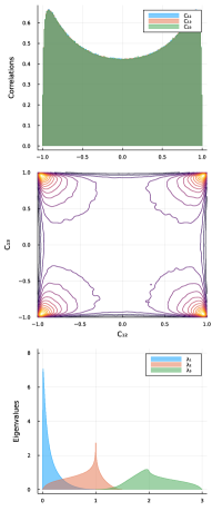
(a) $\gamma\sim N_{3}(0,I)$

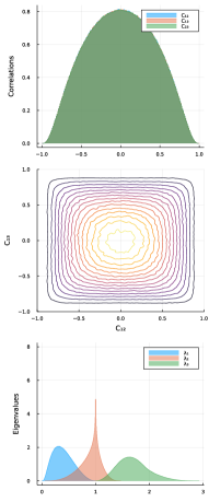
(b) $\gamma\sim N_{3}(0,\tfrac{1}{4}I)$

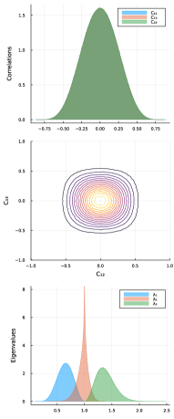
(c) $\gamma\sim N_{3}(0,\tfrac{1}{16}I)$

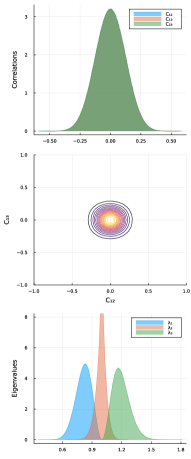
(d) $\gamma\sim N_{3}(0,\tfrac{1}{64}I)$

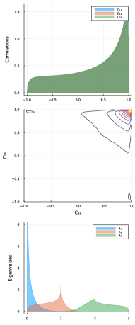
(e) $\gamma\sim N_{3}(\gamma_{0},I)$

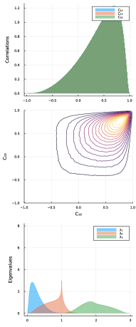
(f) $\gamma\sim N_{3}(\gamma_{0},\tfrac{1}{4}I)$

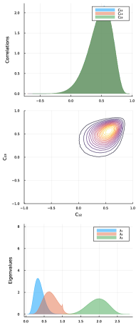
(g) $\gamma\sim N_{3}(\gamma_{0},\tfrac{1}{16}I)$

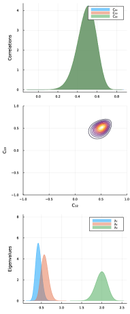
(h) $\gamma\sim N_{3}(\gamma_{0},\tfrac{1}{64}I)$

Figure 1: Properties of random $3\times 3$ correlation matrices generated from $\gamma\sim N_{3}(\gamma_{0},\omega^{2}I)$ with $\gamma_{0}=(\mu,\mu,\mu)^{\prime}$. Upper panels have $\mu=0$ and lower panels have $\mu=\tfrac{1}{3}\log 4$. Panels from left to right have $\omega^{2}=1,\tfrac{1}{4},\tfrac{1}{16}$, and $\tfrac{1}{64}$ respectively. Each panel displays: the marginal distribution of $C_{ij}$; contour plot for the bivariate distribution of $(C_{12},C_{13})$; and the densities of ordered eigenvalues of $C$.

An immediate implication of Theorem 1 is that all of the marginal distributions of the correlations, $C_{ij}$, $i\neq j$ are identical under the stated assumptions. More generally, the vector of correlations in the upper left $m\times m$ principal submatrix, $\varrho=\mathrm{vecl}([C(\gamma)]_{i,j=1,\ldots,m})\in\mathbb{R}^{m(m-1)/2}$, $m\leq n$, has the same distribution as the vector of correlations corresponding to any other principal submatrix, $\tilde{\varrho}=\mathrm{vecl}([C(\gamma)]_{i,j\in\mathcal{I}})$, for some $\mathcal{I}=\{i_{1},\ldots,i_{m}\}\subset\{1,\ldots,n\}$. Under the conditions of Theorem 1, the pairs, $(C_{12},C_{23})$, $(C_{12},C_{13})$, and $(C_{13},C_{23})$, have the same bivariate distribution, but their bivariate distribution need not be identical to that of $(C_{12},C_{34})$, because this pair does not share a common index.

The simplest case to consider in Theorem 1 is $\zeta=\xi_{1}=\cdots=\xi_{n}=0$, such that the element of $\gamma$ are independent and identically distributed. We illustrate the new method for generating random correlation matrices by using this design with independent and Gaussian distributed elements of $\gamma$. Some features of the resulting random correlation matrices are shown in Figure 1 for the case where $n=3$. Panels (a)-(d) correspond to the case where $\gamma_{i}\sim iidN(0,\omega^{2})$, $i=1,2,3$, such that the random correlation matrices are located about $C=I_{3}$. Panels (e)-(h) are based on $\gamma_{i}\sim iidN(\tfrac{1}{3}\log 4,\omega^{2})$. This leads to random correlation matrices in the vicinity of

$$C(\gamma^{\ast})=\left[\begin{array}[]{ccc}1&0.5&0.5\\ 0.5&1&0.5\\ 0.5&0.5&1\end{array}\right],\qquad\text{where}\quad\gamma^{\ast}=\tfrac{\log 4}{3}\left[\begin{array}[]{c}1\\ 1\\ 1\end{array}\right].$$

In each panel of Figure 1, we display (from top to bottom) the marginal distributions for the correlation coefficients, contour plots for bivariate distributions, and the densities for the three eigenvalues. The panels in Figure 1 correspond to the cases where $\omega^{2}=1$, $\tfrac{1}{4}$, $\tfrac{1}{16}$, and $\tfrac{1}{64}$, respectively. From Theorem 1 we know that the marginal distributions are identical when the elements of $\gamma$ are independent, and this can be seen from the simulated densities for $C_{12}$, $C_{13}$, and $C_{23}$, that are indistinguishable in all cases. The contour plots are for the bivariate distribution of $(C_{12},C_{13})$, which are identical to the distributions for any of pair of correlation coefficients as a consequence of Theorem 1.

When the variance of the elements of $\gamma$ is relatively large, $\omega^{2}=1$, then $C(\gamma)$ tends to produce near-singular correlation matrices. This is evident from the distribution of the smallest eigenvalue in Panels (a) and (e), and it can also be seen from the contour plots where the mass in concentrated near the corners of the support for $(C_{12},C_{13})$. As the variance of $\gamma_{i}$ becomes smaller, so does the variance of the resulting correlation coefficients. In Panels (a)-(d), the random correlation matrices become more concentrated about $C(0)=I_{3}$ and in Panels (e)-(h) the random correlations are more concentrated about $\frac{1}{2}$ as $\omega\rightarrow 0$.

2.2 Random Perturbation of Target Correlation Matrix

The new method makes it easy to generate random correlation matrices in the vicinity of a particular correlation matrix. Let $\gamma_{0}=g(C_{0})$ be the vector that corresponds to $C_{0}$ and generate random correlation matrices using $C(\gamma_{0}+\epsilon)$, where $\epsilon$ is a random vector centered about the zero-vector. The dispersion of the random correlation matrices about $C_{0}$ is controlled by the dispersion of $\varepsilon$. We will make use of this property below.

It is important to note that the random correlation matrices are unlikely to have $\mathbb{E}(C)=C_{0}$, because the mapping $C(\gamma)$ is non-linear. However, the discrepancy will be small if the variance of $\varepsilon$ is small.

2.3 Heterogenous Marginal Distributions

In some applications it can be desirable to generate random correlation matrices where the dispersion of the correlation coefficients is heterogeneous. This situation will arise in a Bayesian context if there is stronger prior knowledge about some correlation coefficients than other correlations. The new method can accommodate this situation by using different variances for different elements in $\gamma$. The mapping in (1) is such that its Jacobian, $J_{0}=\mathrm{d}\varrho/\mathrm{d}\gamma\Bigl{|}_{\gamma=\gamma_{0}}$, is approximately a diagonal matrix. Its diagonal elements are all positive and have similar magnitudes, whereas the off-diagonal elements tend to be close to zero. So, increased variance in a particular element of $\gamma$ will primarily induce increased dispersion of the corresponding elements of $\varrho$. For instance, increasing the variance of $\gamma_{1}=[\log C]_{1,2}$ will primarily increase the variance in $\varrho_{1}=C_{1,2}$. There will also be an impact on other correlation coefficients for two reasons. First, the Jacobian only captures a local linear approximation of the mapping, $\gamma\mapsto\varrho=\mathrm{vecl}C(\gamma)$, and second, $J_{0}$ is not perfectly diagonal. This is illustrated in the upper panels of Figure 2. Random correlation matrices were obtained with $\gamma\sim N_{3}(\gamma_{0},\Omega)$, where $\gamma_{0}=\Bigl{(}\frac{1}{4},\frac{1}{4},\frac{1}{4}\Bigl{)}^{\prime}$ and $\Omega=\text{diag}(\tfrac{\omega}{100},\tfrac{1}{100},\tfrac{\omega}{100})$. The resulting contour plots for $(C_{12},C_{13})$, $(C_{12},C_{23})$, and $(C_{13},C_{23})$ are show in the upper panels of Figure 2, where blue solid contour lines correspond to the homogeneous dispersion $(\omega=1)$ and red dashed contour lines represent the heterogeneous case, $\omega=10$, where $\gamma_{1}$ and $\gamma_{2}$ have increased dispersion. In the homogeneous cases the elements of $\gamma$ are independent and identically distributed, which leads to correlations with identical marginal distributions. The three bivariate distributions are also identical because the pair of correlations always have one index in common. We amplified the variance of $\gamma_{1}=G_{12}$ and $\gamma_{3}=G_{23}$ in the heterogeneous case. From the contour plots it is evident that the increased variance of the two elements of $\gamma$ primarily increases the variance of the corresponding correlations $C_{12}$ and $C_{23}$, whereas the effect on $C_{13}$ is modest.

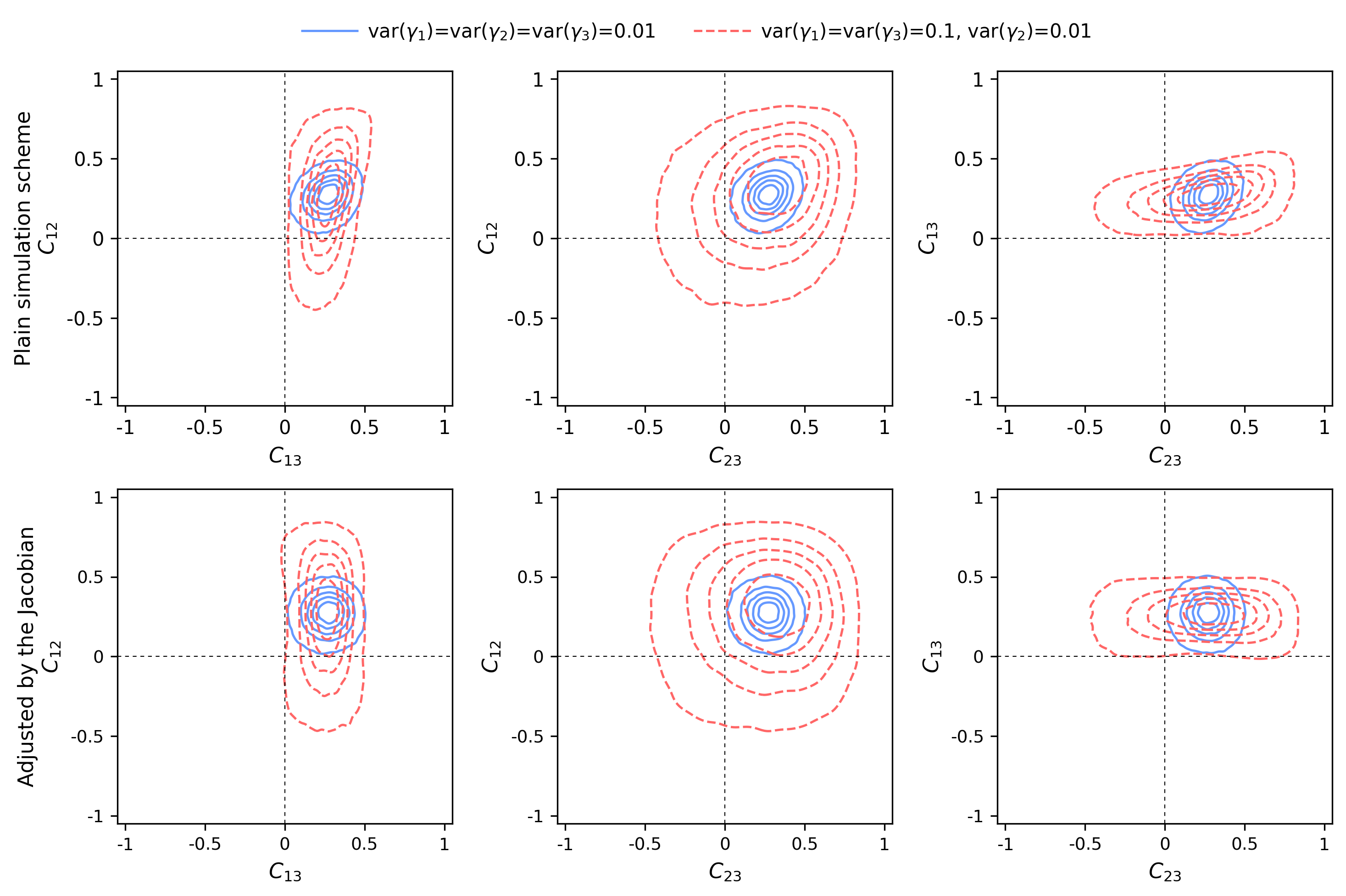
Figure 2: Contour plots for the bivariate distributions for $(C_{12},C_{13})$, $(C_{12},C_{23})$, and $(C_{13},C_{23})$, where $C(\gamma)$ is generated from $\gamma\sim N_{3}(\gamma_{0},\Sigma)$, with $\gamma_{0}=\tfrac{1}{4}(1,1,1)^{\prime}$. Upper panels are with $\Sigma=\Lambda_{\omega}=\text{diag}(\tfrac{\omega}{100},\tfrac{1}{100},\tfrac{\omega}{100})$ and lower panels have $\Sigma=J_{0}^{-1}\Lambda_{\omega}J_{0}^{-1}$ where $J_{0}=\left.\mathrm{d}\varrho/\mathrm{d}\gamma\right|_{\gamma=\gamma_{0}}$ is the Jacobian. Solid blue contour lines are for the homogeneous design with $\omega=1$ and red dashed contour lines are for the heterogeneous case $\omega=10$.

2.4 Additional Dependence Reduction

The Jacobian is not perfectly diagonal and this partly explains the dependence between the correlations, which can be seen in the contour plots in the upper panels of Figure 2. We can account for the structure in $J_{0}$ to reduce the dependence between individual random correlations. From the Taylor expansion, $\varrho(\gamma)\approx\varrho(\gamma_{0})+J_{0}\cdot(\gamma-\gamma_{0}),$ it follows that $\mathrm{var}(\varrho(\gamma))\approx J_{0}\mathrm{var}(\gamma)J_{0}{}^{\prime}$. Therefore, if we set $\mathrm{var}(\gamma)=\Sigma=J_{0}^{-1}\Lambda_{\omega}J_{0}^{-1}$, then $\mathrm{var}(\varrho(\gamma))\approx\Lambda_{\omega}$. This first-order approximation is reliable when $\Sigma=\mathrm{var}(\gamma)$ is small, whereas the nonlinearities in $C(\gamma)$ becomes important if $\Sigma$ is large.

The results based on $\gamma\sim N_{3}(\gamma_{0},J_{0}^{-1}\Lambda_{\omega}J_{0}^{-1})$, with $\gamma_{0}=(\tfrac{1}{4},\tfrac{1}{4},\tfrac{1}{4})^{\prime}$ and $\Lambda_{\omega}=\text{diag}(\tfrac{\omega}{100},\tfrac{1}{100},\tfrac{\omega}{100})$ are presented in the lower panels of Figure 2. The Jacobian and its inverse are (for this $\gamma_{0}$) given by,

$$J_{0}=\left(\begin{array}[]{ccc}0.920&{\color[rgb]{0,.5,.5}0.102}&{\color[rgb]{0,.5,.5}0.102}\\ {\color[rgb]{0,.5,.5}0.102}&0.920&{\color[rgb]{0,.5,.5}0.102}\\ {\color[rgb]{0,.5,.5}0.102}&{\color[rgb]{0,.5,.5}0.102}&0.920\end{array}\right),\qquad\text{and}\quad J_{0}^{-1}=\left(\begin{array}[]{ccc}1.111&{\color[rgb]{.75,0,.25}-0.111}&{\color[rgb]{.75,0,.25}-0.111}\\ {\color[rgb]{.75,0,.25}-0.111}&1.111&{\color[rgb]{.75,0,.25}-0.111}\\ {\color[rgb]{.75,0,.25}-0.111}&{\color[rgb]{.75,0,.25}-0.111}&1.111\end{array}\right),$$

respectively. The solid blue contour lines correspond to the homogeneous case ($\omega=1$) and the red dashed contour lines correspond to the heterogeneous case ($\omega=10$), as in the upper panels. It is not possible to eliminate the dependence between the random correlations entirely. However, the simple Jacobian-based adjustment does reduce the linear dependence, which can be seen by comparing the contour lines in the lower panels with those in the upper panels.

2.5 A Bound for Smallest Eigenvalue of $C(\gamma)$

The new method also makes it simple to bound the smallest eigenvalue of the random correlation matrix, which avoids ill-conditioned matrices. This can be done by bounding the range for the elements of $\gamma$.

Theorem 2.

Let $\gamma_{\max}=\max_{k}|\gamma_{k}|$ be the largest element of $\gamma$ in absolute value. Then,

$$e^{-K\gamma_{\max}}\leq\lambda_{\min}\leq e^{-\gamma_{\max}},$$

for some $K<\infty$.

The first inequality in Theorem 2 shows that the smallest eigenvalue of $C(\gamma)$ is bounded away from zero by placing a bound on $\max_{k}|\gamma_{k}|$, and we conjecture that $K=n$. Interestingly, we note that $\exp(\text{\textminus}n\gamma_{\max})\simeq\tfrac{ne^{-n\gamma_{\max}}}{n-1+e^{-n\gamma_{\max}}}$ for large values of $\gamma_{\max}$, where the latter is the smallest eigenvalue of an equicorrelation matrix with a common negative correlation.

In Figure 3 we have plotted $\log\lambda_{\min}$ against $-\gamma_{\max}$ for one million random correlation matrices with dimension $n=5$ along with the conjectured upper and lower bound for $\log\lambda_{\min}$. The lower bound appears to be binding for very large values of $\gamma_{\max}$, whereas the upper bound only becomes binding for $\gamma_{\max}\simeq 0$. The latter corresponds to the case where $C\simeq I$.

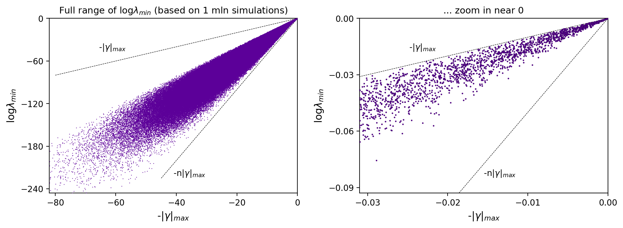
Figure 3: Scatter plots of $\log\lambda_{\min}$ against $-\gamma_{\max}$ for one million random $5\times 5$ correlation matrices.

2.6 Resembling the Distribution of Empirical Correlation Matrices

The method can be used to approximate the distribution of empirical correlation matrices. Let $\hat{C}$ be an empirical correlation matrix computed from $T$ observations and consider $\hat{\gamma}=g(\hat{C})$. Under suitable regularity conditions, Archakov & Hansen (2021a) showed that $\sqrt{T}(\hat{\gamma}-\gamma)\overset{d}{\rightarrow}N(0,V_{\gamma})$ and derived an expression for $V_{\gamma}$. This asymptotic approximation works well in finite samples and the off-diagonal elements of $V_{\gamma}$ tend to be close to zero, especially for high-dimensional correlation matrices, see Archakov & Hansen (2020). This suggests that the new method can be used to resemble the distributions of empirical correlation matrices by drawing $\gamma$ from a suitable Gaussian distribution.

3 Random Correlation Matrices with Special Structures

3.1 Non-Negative and Positive Random Correlation Matrices

In this section, we show that non-negative correlations are guaranteed if all elements of $\gamma$ are non-negative, and strictly positive correlation are guaranteed if the elements of $\gamma$ are strictly positive. The latter would, by the Perron-Frobenius theorem, ensure that the eigenvector associated with the largest eigenvalue of $C$ had strictly positive elements.

We borrow some terminology from the Markov chain literature for the purpose of generating non-negative and positive correlation matrices.

Definition 1.

An $n\times n$ matrix, $A$, is reducible if there exists a permutation matrix, $P$, such that $B=PAP^{\prime}=\left[\begin{array}[]{cc}B_{[1,1]}&B_{[1,2]}\\ B_{[2,1]}&B_{[2,2]}\end{array}\right]$ has $B_{[2,1]}=0_{n_{2}\times n_{1}}$, where $n_{1},n_{2}\geq 1$ and $n_{1}+n_{2}=n$, otherwise $A$ is said to be irreducible.

Because a correlation matrix is symmetric, it follows that $C=\mathrm{corr}(X)$ is reducible if and only if the variables can be reordered, $\tilde{X}=PX$, such that $\tilde{C}=\mathrm{corr}(\tilde{X})$ is a block diagonal matrix, i.e.

$$\tilde{C}=PCP^{\prime}=\left[\begin{array}[]{cc}\tilde{C}_{[1,1]}&0\\ 0&\tilde{C}_{[2,2]}\end{array}\right],$$

in which case we observe that

$$\tilde{G}=\log\tilde{C}=\left[\begin{array}[]{cc}\log\tilde{C}_{[1,1]}&0\\ 0&\log\tilde{C}_{[2,2]}\end{array}\right],$$

has the same block diagonal structure. This shows that $C$ is reducible if and only if $G$ is reducible.

Theorem 3.

If $\gamma_{k}\geq 0$ for all $k=1,\ldots,d$, then all elements of $C(\gamma)$ are non-negative. Moreover, if $G(\gamma)=\log C(\gamma)$ is irreducible then all elements of $C(\gamma)$ are strictly positive.

An implication of Theorem 3 is that $\gamma_{k}>0$ for all $k$ will translate to a $C(\gamma)$ with strictly positive elements, because $G(\gamma)$ is irreducible in this case.

It is worth mentioning that $\tilde{\gamma}\geq\gamma\geq 0$ $\centernot\implies$ $C(\tilde{\gamma})\geq C(\gamma)$, as illustrated with the following counterexample:

$$C(\left[\begin{array}[]{c}0.60\\ 1.50\\ 0.05\end{array}\right])=\left[\begin{array}[]{ccc}1&0.507&0.897\\ 0.507&1&0.325\\ 0.897&0.325&1\end{array}\right],\qquad C(\left[\begin{array}[]{c}0.59\\ 0.50\\ 0.04\end{array}\right])=\left[\begin{array}[]{ccc}1&0.528&0.460\\ 0.528&1&0.166\\ 0.460&0.166&1\end{array}\right].$$

3.2 Equicorrelation Matrices

An equicorrelation matrix, $C$, is a correlation matrix where all the correlations are identical. The corresponding $\gamma=g(C)$ is a vector whose elements have the same value. Let $r$ denoted the common correlation coefficient in $C$ and let $z$ be the corresponding common element of $\gamma$, then the relationship between the two is given by,

$$z(r)=\frac{1}{n}\log\left(1+n\tfrac{r}{1-r}\right),$$ (3)

and the inverse transformation is $r(z)=\frac{1-e^{-nz}}{1+(n-1)e^{-nz}}$, see e.g. Archakov & Hansen (2021a). An equicorrelation matrix has two eigenvalues, $1+r(n-1)$ and $1-r$, where the latter has multiplicity $n-1$, see Olkin & Pratt (1958). Thus, the $n\times n$ equicorrelation matrix is positive definite if and only if $r\in(-\tfrac{1}{n-1},1)$.

The following theorem establishes a relationship between the Beta distribution for $r$ and a generalized logistic distribution for $z$.

Theorem 4.

Let $\gamma=(z,\ldots,z)^{\prime}\in\mathbb{R}^{d}$ with $d=n(n-1)/2$. Then $C(\gamma)$ is an equicorrelation matrix, where the common correlation coefficient, $r$, is confined to the interval $(-\tfrac{1}{n-1},1)$ for all $z\in\mathbb{R}$. Moreover, if $z$ has density,

$$f_{z}(z)=\frac{1}{B(\alpha,\beta)}\frac{e^{-\beta\tfrac{z-\mu}{s}}}{s\left(1+e^{-\tfrac{z-\mu}{s}}\right)^{\alpha+\beta}},\qquad z\in\mathbb{R},$$ (4)

where $\mu=\tfrac{\log(n-1)}{n}$ and $s=\tfrac{1}{n}$, then $r$ is Beta distributed, $B(\alpha,\beta)$, on the interval $(-\tfrac{1}{n-1},1)$.

The density (4) was introduced in Prentice (1975) and is known as the Generalized Logistic Distribution of Type IV. This distribution is also referred to as the Exponential Generalized Beta distribution of the second type, see e.g. Caivano & Harvey (2014).

If we set $\alpha=\beta=1$, it follows immediately that $r$ is uniformly distributed on $(-\tfrac{1}{n-1},1)$.

Corollary 1.

Let $\gamma=(z,\ldots,z)^{\prime}\in\mathbb{R}^{d}$ with $d=n(n-1)/2$, and suppose that $z$ is logistically distributed,

$$f_{z}(z)=\frac{e^{-\tfrac{z-\mu}{s}}}{s\left(1+e^{-\tfrac{z-\mu}{s}}\right)^{2}},\qquad z\in\mathbb{R},$$ (5)

where $\mu=\tfrac{\log(n-1)}{n}$ and $s=\tfrac{1}{n}$, then $r$ is uniformly distributed on the interval $(-\tfrac{1}{n-1},1)$.

In the special case where $n=2$, we have $\mu=0$ and $s=1/2$ and the logistic distribution in (5) is also known as a Fisher $z$-distribution with $(d_{1},d_{2})=(2,2)$ degrees of freedom.

Theorem 4 provides valuable insight about the dispersion of the elements of $\gamma$ as the dimension of the correlation matrix, $n$, increases. The variance for the density in (5) is $\mathrm{var}(z)=\frac{\pi^{2}}{3}n^{-2}$. This suggests that a scaling factor of $1/n$ should be used on the elements of $\gamma$ to preserve similar dispersion for the correlation coefficients in $C(\gamma)$ as $n$ increases.

3.3 Block Correlation Matrices

If $C$ has a block structure then $\log C$ and $C^{-1}$ has the same block structure, see Archakov & Hansen (2022). This can be used to generate random correlation matrices with block structures, as well as random precision matrices, $C^{-1}$, with block structures, while positive definiteness is guaranteed. A correlation matrix has a block structure if

$$C=\left[\begin{array}[]{cccc}C_{[1,1]}&C_{[1,2]}&\cdots&C_{[1,K]}\\ C_{[2,1]}&C_{[2,2]}\\ \vdots&&\ddots\\ C_{[K,1]}&&&C_{[K,K]}\end{array}\right]\in\mathbb{R}^{n\times n},$$

where the diagonal blocks, $C_{[i,i]}\in\mathbb{R}^{n_{i}\times n_{i}}$, where $i=1,...,K$, have ones along the diagonal and $\rho_{i,i}\in(-1,1)$ in all off-diagonal elements (i.e., equicorrelation structure), and the off-diagonal blocks, $C_{[i,j]}\in\mathbb{R}^{n_{i}\times n_{j}}$, where $i,j=1,\ldots,K$ and $i\neq j$, $n_{1}+\cdots+n_{K}=n$ have all elements equal to $\rho_{i,j}\in(-1,1)$. Symmetry is guaranteed with $\rho_{i,j}=\rho_{j,i}$.The values $\rho_{i,j}$ must also be such that $C$ is a positive definite matrix.

A useful property of this structure is that the matrix logarithm, $G=\log C$, is also a block matrix with the same block structure as $C$. Thus,

$$G_{[k,k]}=\left[\begin{array}[]{cccc}y_{k}&\gamma_{k,k}&\cdots&\gamma_{k,k}\\ \gamma_{k,k}&y_{k}&\ddots&\vdots\\ \vdots&\ddots&\ddots&\gamma_{k,k}\\ \gamma_{k,k}&\cdots&\gamma_{k,k}&y_{k}\end{array}\right]\in\mathbb{R}^{n_{k}\times n_{k}}\qquad G_{[k,l]}=\left[\begin{array}[]{ccc}\gamma_{k,l}&\cdots&\gamma_{k,l}\\ \vdots&\ddots&\vdots\\ \gamma_{k,l}&\cdots&\gamma_{k,l}\end{array}\right]\in\mathbb{R}^{n_{k}\times n_{l}},\quad k\neq l,$$ (6)

with $\gamma_{k,l}\in\mathbb{R}$ and $\gamma_{k,l}=\gamma_{l,k}$ for $i,j=1,\ldots,K$. Matrix $C$ is uniquely determined from the off-diagonal elements of $G$, and the inverse mapping can be obtained with the algorithm in Archakov & Hansen (2021a). The problem is to determine a $n\times 1$ diagonal vector for $G$ such that $\exp\{G\}$ is a correlation matrix. Generally, it requires the matrix exponential to be evaluated for an $n\times n$ matrix (several times) and the computational burden of this is of order $\mathcal{O}(n^{3}\log n)$. For block matrices, the entries on the main diagonal are identical within each diagonal block, so we have to determine only $K$ diagonal elements, $y=(y_{1},...,y_{K})^{\prime}$, which greatly simplifies the computational burden.

The matrix $G$ can be represented as $G=QDQ^{\prime}$, where $Q$ is an orthonormal matrix, $Q^{\prime}Q=I_{n}$, which does not depend on the elements of $C$ (nor $G$). The corresponding closed-form expression for $D$ is

$$D=\left[\begin{array}[]{cccc}A+\mathrm{diag}(y)&0&\cdots&0\\ 0&(y_{1}-\gamma_{1,1})I_{n_{1}-1}&&\vdots\\ \vdots&&\ddots&0\\ 0&\cdots&0&(y_{K}-\gamma_{K,K})I_{n_{K}-1}\end{array}\right],$$ (7)

where $A$ is a $K\times K$ matrix with elements,

$$A_{k,l}=\begin{cases}\gamma_{k,k}(n_{k}-1)&\text{for }k=l,\\ \gamma_{k,l}\sqrt{n_{k}n_{l}}&\text{for }k\neq l,\end{cases}$$

and $\mathrm{diag}(y)$ is the $K\times K$ diagonal matrix with the elements of $y$ along the diagonal, see Archakov & Hansen (2022) for details. In this representation, all distinct off-diagonal entries of $G$ appear in $K\times K$ upper left diagonal block of $D$. This is convenient, as it can be shown that to restore the original matrix $C$ from given values $\gamma_{k,l}$, we only need to find a proper vector $y$ which determines the diagonal of this block as well as the entire main diagonal of $D$.

Theorem 5.

Let $G$ be of the form (6) for some $n_{1},\ldots,n_{K}\in\mathbb{N}$. Given any constants, $\gamma_{k,l}\in\mathbb{R}$, $1\leq k,l\leq K$, with $\gamma_{k,l}=\gamma_{l,k}$, there exist unique constants, $y_{1}^{\ast},\ldots,y_{K}^{\ast}\leq 0$, such that $\exp G[y]$ is a block correlation matrix. The unique $y^{\ast}$ can be determined by iterating on,

$$y_{k}^{(N+1)}=y_{k}^{(N)}+\log n_{k}-\log\left([\exp\{A+\mathrm{diag}(y^{(N)})\}]_{kk}+(n_{k}-1)\,e^{y_{k}^{(N)}-\gamma_{k,k}}\right),$$

until convergence from an arbitrary starting value, $y^{(0)}\in\mathbb{R}^{K}$.

The computational burden of this algorithm is of order $\mathcal{O}(K^{3}\log K)$, which is a substantial simplification relative to the generic algorithm in Archakov & Hansen (2021a) whenever $K$ is smaller than $n$. Theorem 5 shows that in order to generate a random block correlation matrix, it suffices to generate the off-diagonal entries of $G$, $\gamma_{k,l}\in\mathbb{R}$, and then recover the unique vector $y^{\ast}\in\mathbb{R}^{K}$. The algorithm in Theorem 5 ensures that $\exp G[y^{*}]$ has ones along the main diagonal and is a valid block-correlation matrix. Moreover, all elements of $C=\exp G[y^{*}]$ are available in a closed-form as functions of $\gamma_{k,l}$ and $y^{*}$. An evaluation of matrix exponential for the $n\times n$ matrix $G[y^{*}]$ is not needed.

It is straight forward to generate random block correlation matrices in the vicinity of a particular block correlation matrix using the method described here, and it is obviously also possible to generate random correlation matrices (without a block structure) in the vicinity of a particular block correlation matrix using the standard algorithm proposed in Archakov & Hansen (2021a).

3.3.1 Random correlation matrices of (very) large dimensions

The canonical representation of block matrices can also be used to efficiently generate high-dimensional correlation matrices by taking convex combinations of permutated random block matrices, i.e.,

$$C=\sum_{m=1}^{M}\omega_{m}P_{m}Q\exp\{D_{m}\}Q^{\prime}P_{m}^{\prime},\qquad\sum_{m}\omega_{m}=1,\quad\omega_{m}\geq 0,$$

where $D_{m}$, $m=1,\ldots,M$ are constructed from random $\gamma_{k,l}$, $1\leq k\leq l\leq K$ with the block structure (7) and $P_{m}$ are perturbation matrices. Figure 4 presents random $250\times 250$ correlation matrices, which are constructed from $M=1$ (upper plots), $M=2$ (middle plots) and $M=10$ (bottom plots) random block correlation matrices, each having $5\times 5$ blocks (each block is of size $50\times 50$), such that each block correlation matrix has 15 distinct correlation coefficients. Before averaging the matrices, the rows (and columns) are shuffled with random perturbations. The resulting matrices are guaranteed to be positive definite, and the corresponding smallest eigenvalues are also reported in the Figure. As we can observe, the generated random matrix fastly departs from the block structure as $M$ increases, which is manifested by the diversity of the corresponding correlation elements rising quickly with $M$.

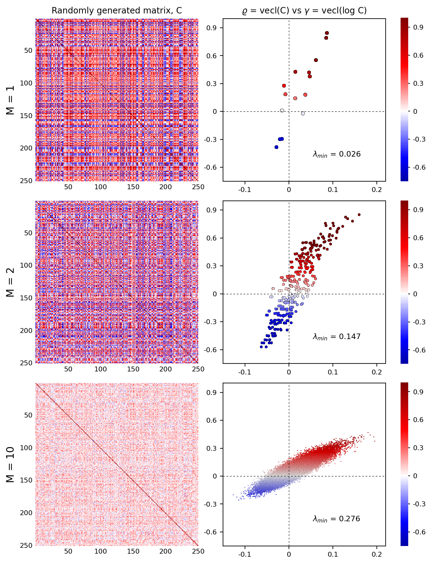
Figure 4: The left side presents random $250\times 250$ correlation matrices, $C$, constructed as the average of 1, 2 and 10 random block matrices, whose rows and columns were subject to random permutations. The right side presents scatter plots with the corresponding correlation elements contained in the resulting matrices ($\varrho=\text{vecl}(C)$ are drawn against $\gamma=\text{vecl}(\log C)$).

4 Existing Methods for Generating Random Correlation Matrices

There is a large literature on generating random correlation matrices, see Marsaglia & Olkin (1984) and Pourahmadi (2011) for references. In this section, we discuss some existing methods for generating random correlation matrices, and compare some of their features and properties with those of the new method.

4.1 Naive Method

A simple method to generate random correlation matrices is to simply generate random correlation coefficients, $C_{i,j}\in[-1,1]$, $1\leq i<j\leq n$, set $C_{ii}=1,$ for $i=1,\ldots n$, $C_{i,j}=C_{j,i}$ for $i<j$, and then discard the invalid correlation matrices, which are characterized by $\lambda_{\min}(C)<0$.

This approach yields a uniform distribution over the set of valid correlation matrices when $C_{ij}$, $1\leq i\leq j\leq n$ are independent and uniformly distributed on $[-1,1]$. Interestingly, the correlation coefficients, $C_{i,j}$, in the retained correlation matrices are beta distributed on $[-1,1]$, $B(\alpha,\alpha)$ with $\alpha=n/2$. This can be inferred from results in Joe (2006). This naive method for generating random correlation matrices is very inefficient and impractical except for very low dimensional matrices. With $n=6$ the percentage of matrices with negative eigenvalues is more than 99.9%, and for $n=10$ it takes about 55 quadrillions random matrices to get a single valid correlation matrix, see Figure 5. This approach clearly impractical except for small $n$.

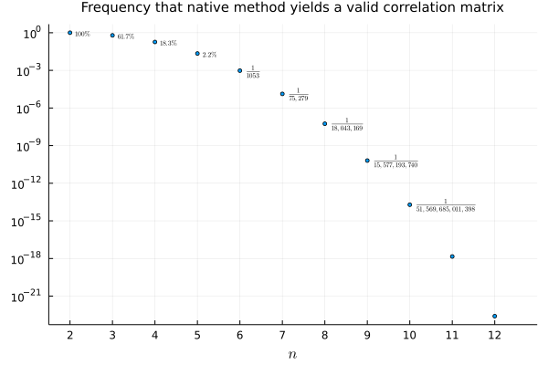
Figure 5: The probability that a symmetric matrix with independent and uniformly distributed elements, $C_{ij}$, $1\leq i<j\leq n$ on $[-1,1]$, and $C_{ii}=1$, $i=1,\ldots,n$, is a valid correlation matrix.

4.2 Random Gram Methods

A valid correlation matrix can be obtained from any $m\times n$ matrix, $U=(u_{1},\ldots,u_{n})$, with normalized columns, $u_{j}^{\prime}u_{j}=1$, for $j=1,\ldots,n$. It follows immediately that $C=U^{\prime}U$ is positive semidefinite with ones along the diagonal, and if $U$ has rank $n$, then $C=U^{\prime}U$ is a non-singular correlation matrix. Several methods are based on this idea (typically with $m=n$), where a random correlation matrix is obtained from random vectors, $u_{1},\ldots,u_{n}$, on the unit sphere, $S_{m}=\{u\in\mathbb{R}^{m},u^{\prime}u=1\}$. The random Gram method generates $n$ vectors on $S_{n}$ and the Gram matrix $C=U^{\prime}U$ is the resulting random correlation matrix. The uniform distribution on $S_{n}$ was discussed in Marsaglia & Olkin (1984), see also Holmes (1991), and it generates a $C$ where the marginal distributions of the correlation coefficients are Beta distributed, $B(\frac{1}{2},\frac{n-1}{2})$. The vectors, $u_{j},$ $j=1,\ldots,n$, can be drawn from other distributions, such as those proposed by Tuitman et al. (2020), which ensures that the average correlation coefficient is centered about a particular value.

4.3 Standard Angles Parameterization (SAP) Method

A variant of the Random Gram method is the case where $U$ is a triangular matrix. This choice was discussed in Marsaglia & Olkin (1984) and a particular triangular form was proposed by Pinheiro & Bates (1996). Their choice for $U$ is defined by the angles, $\theta_{ij}\in[0,\pi)$, for $1\leq i<j\leq n$, such that

$$U=\left[\begin{array}[]{cccccc}1&\cos\theta_{1,2}&\cos\theta_{1,3}&\cdots&\cos\theta_{1,n-1}&\cos\theta_{1,n}\\ 0&\sin\theta_{1,2}&\cos\theta_{2,3}\sin\theta_{1,3}&\cdots&\cos\theta_{2,n-1}\sin\theta_{1,n-1}&\cos\theta_{2,n}\sin\theta_{1,n}\\ 0&0&\Pi_{i=1}^{2}\sin\theta_{i,3}&&\cos\theta_{3,n-1}\Pi_{i=1}^{2}\sin\theta_{i,n-1}&\cos\theta_{3,n}\Pi_{i=1}^{2}\sin\theta_{i,n}\\ \vdots&\vdots&\ddots&\ddots&&\vdots\\ 0&0&0&&\Pi_{i=1}^{n-2}\sin\theta_{i,n-1}&\cos\theta_{n-1,n}\Pi_{i=1}^{n-2}\sin\theta_{i,n}\\ 0&0&0&\cdots&0&\Pi_{i=1}^{n-1}\sin\theta_{i,n}\end{array}\right]$$

is an upper triangular matrix. This requires $d=n(n-1)/2$ angles, $\theta_{ij}$, and it follows that any distribution on $[0,\pi)^{d}$ will correspond to some distribution over the space of correlation matrices. If the angles are independent and uniformly distributed on $[0,\pi)$, then $C$ has coefficients with very heterogeneous marginal distributions. If one instead specifies $\theta_{ij}$ to have the density

$$f_{j}(x;\alpha)=\frac{\sin^{2\alpha-j}(x)}{B(\alpha-\frac{j-1}{2},\frac{1}{2})},\qquad j=1,\dots,n-1,$$

for some $\alpha\geq n/2$, then marginal distributions of the correlation coefficients are identical and Beta distributed, $\mathrm{Beta}(\alpha,\alpha)$ on the interval $[-1,1]$, see Pourahmadi & Wang (2015). This is known as the Standard Angles Parameterization (SAP) method.

4.4 Eigendecomposition Method

One of the first ways to generate random correlation matrices, see Chalmers (1975) and Bendel & Mickey (1978), was based on the eigendecomposition of the correlation matrix, $C=Q\Lambda Q^{\prime}$ where $Q^{\prime}Q=I$ and $\Lambda=\mathrm{diag}(\lambda_{1},\ldots,\lambda_{n})$.

The premise of this method is a distribution of eigenvalues on the $n$-simplex: $\{(\lambda_{1},\ldots,\lambda_{n}):\sum_{j}\lambda_{j}=n,\text{ }\lambda_{j}\geq 0\}$. Given a set of random eigenvalues, the method proceeds to determine a set of eigenvectors (the columns of $Q$), such that $Q\Lambda Q^{\prime}$ is a valid correlation matrix. The latter is not a trivial step, because the set of $Q$ matrices that produce a valid correlation matrix for a given set of eigenvalues has measure zero in the set of all orthonormal matrices. For the pair $(\Lambda,Q)$ to generate a valid correlation matrix, the following conditions must be satisfied.

1. The diagonal matrix, $\Lambda$, must satisfy $\lambda_{j}\geq 0$, $j=1,\ldots,n$, and $\sum_{j=1}^{n}\lambda_{j}=n$.

2. The matrix $Q=(q_{1},\ldots,q_{n})$ must be orthonormal, $q_{j}^{\prime}q_{j}=1$ and $q_{i}^{\prime}q_{j}=0$ for all $i\neq j=1,\ldots,n$.

3. Combined they must satisfy $\mathrm{diag}(Q\Lambda Q^{\prime})=(1,\ldots,1)^{\prime}$ .

The last condition is a cross restriction on $\Lambda$ and $Q$. Among all $Q$-matrices that satisfy the second condition, the fraction of matrices that also satisfy the third condition for a particular $\Lambda$, is zero. A method for determining a valid $Q$-matrix is therefore needed, and such algorithms are given in Chalmers (1975), Bendel & Mickey (1978), Marsaglia & Olkin (1984), and Davies & Higham (2000). These methods begin with an initial (random) orthonormal matrix, $Q_{0}$, that is subjected to successive transformations until a valid $Q$-matrix is determined. The method by Davies & Higham (2000) is implemented in the MATLAB function gallery(’randcorr’).

4.5 Partial Correlations (PAC) Method

The partial correlation (PAC) method by Joe (2006) uses random partial correlations to generate random correlation matrices. Specifically the $n(n-1)/2$ partial correlations given by

$$\varrho_{ij}=\frac{C_{ij}-d_{ij}^{(i,j)}}{\sqrt{(1-d_{ii}^{(i,j)})(1-d_{jj}^{(i,j)})}},\qquad\text{for}\quad 1\leq i<j\leq n,$$

where $d_{ij}^{(i,j)}=C_{i,I_{ij}}[C_{I_{ij},I_{ij}}]^{-1}C_{I_{ij},j}$, and $C_{I_{ij},I_{ij}}=[C_{l,m}]_{i<l,m<j}$, $C_{i,I_{ij}}=[C_{i,m}]_{i<m<j}$, and $C_{I_{ij},j}=C_{j,I_{ij}}^{\prime}$, are sub-matrices of $C$. When $j=i+1$ the partial correlation is simply the correlation, $\varrho_{i,i+1}=C_{i,i+1}$; otherwise, $\varrho_{ij}$ is the partial correlation between the $i$-th and $j$-th variables, conditional on all variables indexed between $i$ and $j$. Clearly any correlation matrix, $C$, will map to $\{\varrho_{i,j}\}_{1\leq i<j\leq n}$ and any set of these partial correlation in $(-1,1)$ will translate to a valid correlation matrix. This is similar to the result for stationary time series derived in Barndorff-Nielsen & Schou (1973). Lewandowski et al. (2009) builds on Joe (2006) to propose computationally fast ways to generate high-dimensional random correlation matrices.

Interestingly, the determinant of $C$ is given by $\det C=\prod_{1\leq i<j\leq n}(1-\varrho_{ij}^{2})$, see Joe (2006, theorem 1). The PAC method draws from a distribution on $(-1,1)^{d}$, with $d=n(n-1)/2$, and reconstructs the correlations from the partial correlations.

When the partial correlations, $\{\varrho_{i,j}\}_{1\leq i<j\leq n}$, are drawn independently and from the Beta distribution, $\mathrm{Beta}(\alpha_{ij},\alpha_{ij})$ on $(-1,1)$, with $\alpha_{ij}=\alpha+(1-j+i)/2$, then the correlation coefficients are identically distributed with $C_{ij}\sim\mathrm{Beta}(\alpha,\alpha)$, where $\alpha>(n-2)/2$, see Joe (2006). Moreover, the joint density of all correlations becomes proportional to the determinant of the correlation matrix to the power $\alpha-n/2$. It follows that by setting $\alpha=n/2$, this method will generate the same distribution as the naive method.

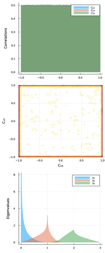
(a) Random Gram

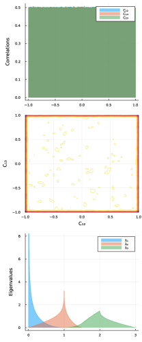
(b) PAC/SAP ($\alpha=1$)

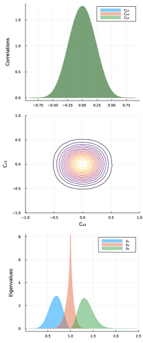
(c) PAC/SAP ($\alpha=10$)

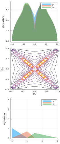
(d) Eigendecomposition

Figure 6: Properties of four existing methods for generating random correlation matrices for the case $n=3$. (a) Random Gram with uniform distribution on the sphere; (b,c) SAP and PAC methods with $\alpha=1$; (d) Bendel and Mickey’s method with eigenvalues $\lambda_{i}=y_{i}/(y_{1}+y_{2}+y_{3})$, $i=1,\ldots,3$, with $y_{i}$ iid and distributed as Exp(1). Marginal distributions are show for $C_{12}$, $C_{13}$, and $C_{23}$ (top) and $\lambda_{1}$, $\lambda_{2}$, and $\lambda_{3}$(bottom), and contour plots for bivariate density of $(C_{12},C_{13})$ is shown in the middle panels.

The properties of some random correlation matrices, $n=3$, are shown in Figure 6. Panel (a) is the Random Gram method where $u_{j}$, $j=1,\ldots,3$ are independent and uniformly distributed on the sphere, $S_{3}$. This choice yields uniformly distributed correlation coefficients when $n=3$. Panels (b) and (c) are the distributions that the SAP and PAC methods produce with $\alpha=1$ and $\alpha=10$, respectively. Panel (d) is the eigendecomposition-based method and it produces rather bizarre marginal and joint distributions for the correlations. This suggests that the algorithm used to determine a valid orthonormal matrix, $Q$, results in some unexpected patterns in the distribution for $C$. The marginal distributions are heterogeneous and there are odd dependencies between correlation coefficients. We have investigated this aspect of the eigendecomposition-based method for $n=5$ in Figure 7. It also shows very heterogeneous and bimodal marginal distributions and rather bizarre and heterogeneous contour plots for pairs of correlations, including multimodal joint distributions.

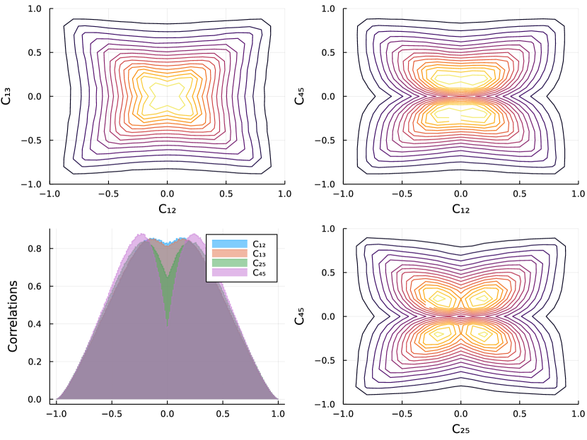
Figure 7: Properties of eigendecomposition-based method for generating random correlation matrices when $n=5$. Marginal distributions for four correlations are shown in the lower-left panel and the three other panels display contour plots for three bivariate distributions.

4.6 Random Correlations from Matrix Distributions

Another popular approach for generating random covariance and correlation matrices is based on the Wishart distribution and, more generally, the matrix Gamma distribution. This method, which we will refer to as the Wishart method, is frequently used in a Bayesian context. The Wishart distribution is defined over symmetric positive semi-definite matrices and arises as the distribution of a scaled sample covariance matrix obtained from a sample of Normal random vectors. For instance, if $X_{t}\sim\mathrm{iid}N_{n}(0,\Sigma)$, $t=1,...,T$, then $S=\sum_{t=1}^{T}X_{t}X_{t}^{\prime}$ is Wishart distributed with parameters $\Sigma$ and $T$, written $S\sim\mathcal{W}_{n}(\Sigma,T)$, where $T$ is the degrees of freedom parameter. We have that $\frac{1}{T}S$ is a sample covariance matrix, and the corresponding sample correlation matrix is $\hat{C}=D_{S}^{-1}SD_{S}^{-1}$, where $D_{S}=\text{diag}\bigl{(}S_{11}^{\frac{1}{2}},...,S_{nn}^{\frac{1}{2}}\bigl{)}$. Thus, generating a random correlation matrix from the Wishart distribution, $\mathcal{W}_{n}(\Sigma,T)$, is equivalent to computing a sample correlation matrix, $\hat{C}$, from a random sample, $X_{t}\sim\mathrm{iid}N_{n}(0,\Sigma)$, $t=1,...,T$. For $\hat{C}$ to be non-singular, the sample size, $T$, must be at least as large as the matrix dimension, $n$.

Generating a random correlation matrix in a vicinity of a target correlation matrix, $C$, is possible with the Wishart method. This can be done using $S=\sum_{t=1}^{T}X_{t}X_{t}^{\prime}$ where $X_{t}\sim\mathrm{iid}N_{n}(0,C)$, $t=1,...,T$. However, there are some drawbacks to the Wishart method. First, the possible range of dispersions for the individual correlations is severely limited by the constraint: $T\geq n$. We have $\sqrt{T}(\hat{C}_{ij}-C_{ij})\overset{d}{\rightarrow}N(0,(1-C_{ij}^{2})^{2})$, as $T\rightarrow\infty$, such that for large $T$, the random correlation $\hat{C}_{ij}$ will be approximately distribution as $N(C_{ij},\frac{(1-C_{ij}^{2})^{2}}{T})$, which shows that $\mathrm{var}(\hat{C}_{ij})$ is (approximately) bounded to be below $\frac{1}{n}(1-C_{ij}^{2})^{2}$. Another implication is that it is not possible to control the relative dispersion of different elements of $C$ with the Wishart method; their variance is given from $C$ and $T$, and their relative variance is asymptotically determined from $C$ alone.

The new method for generating random correlation matrices makes it possible emulate the Wishart method. This is achieved with a single random vector, $\gamma$, drawn from the appropriate Gaussian distribution, see Section 2.6. An advantage of the new method is that it is not bounded by the limitations of the Wishart method, and the new method makes it simple to control the relative dispersion of elements in $C$, as discussed in Section 2.3.

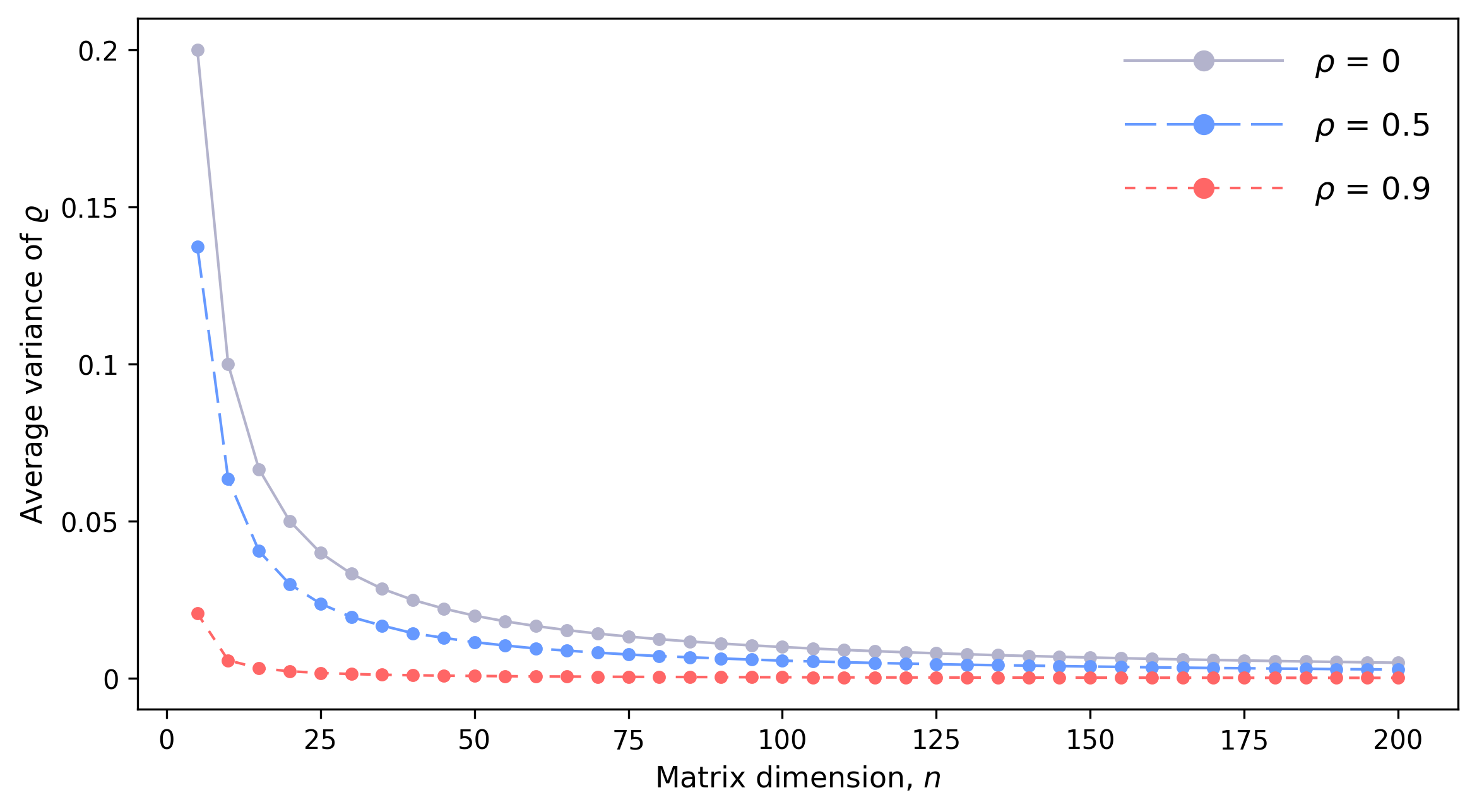
Figure 8: Average variances of elements in random correlation matrices generated by the Wishart method, $\mathcal{W}_{n}(C,n)$, as a function of the dimension $n$, where the target matrix, $C$, is an equicorrelation matrix with $\rho=0.0$, $0.5$, and $0.9$.

The limitations of the Wishart method is illustrated in Figure 8. For a range of matrix dimensions, $n$, we generate random Wishart correlation matrices with $T=n$, which corresponds to the largest possible dispersion of the random correlations. For the target correlation matrix we use equicorrelation matrices with $\rho=0$, $\rho=0.5$, and $\rho=0.9$. Figure 8 presents the variance of random correlation coefficients using the Wishart method for the three target matrices. The upper bound for the variance drops rapidly as $n$ increases, especially for $\rho=0.9$.

5 Summary

In this paper, we have introduced a new method for generating random correlation matrices. The method is based on a one-to-one mapping between the space of non-singular correlation matrices, $\mathcal{C}_{n\times n}$, and the space of real vectors, $\mathbb{R}^{d}$, where $d=n(n-1)/2$. Any distribution on $\mathbb{R}^{d}$ translates to a distribution on $\mathcal{C}_{n\times n}$ (and vice versa). The method is simple: draw a random vector, $\gamma$, and evaluate $C(\gamma)$. The correlation matrix is guaranteed to be positive definite without the need for additional restrictions.

The new method provides a unified framework for generating random correlation matrices, including correlation matrices with special structures. The new method makes it easy to generate random correlation matrices with wide range of properties: strictly positive elements, block structures, well-conditioned, in the vicinity of a particular correlation matrix, and containing elements with similar or heterogeneous dispersions. In some applications is will be natural for the distribution on $\mathcal{C}_{n\times n}$ to be invariant to the ordering of the variables. This would, among other things, imply that the marginal distributions of the correlation coefficients are identical. This invariance property is also simple to satisfy with the new method. Theorem 1 characterizes the class of distributions for $\gamma$ that leads to random correlation matrices with this property. Finally, the proposed framework can be used to generate high dimensional random correlation matrices in a way that is computationally efficient.

We have reviewed several existing methods for generating random correlation matrices. We discussed their advantages and limitations which may be helpful for selecting the method that is best suited for practical application. We also identified some peculiar properties of the commonly used Bendel-Mickey method.

Appendix A Appendix of Proofs

Proof of Theorem 1. Set $G=\log C(\gamma)$ and consider $\tilde{G}=(PGP)$. Since $G_{ij}=h(\varepsilon_{ij},\xi_{i},\xi_{j},\xi_{0})$ it follows that $\gamma=\mathrm{vecl}(G)$ and $\tilde{\gamma}=\mathrm{vecl}(\tilde{G})$ are identically distributed for any permutation matrix, $P$. Consequently, $C=C(\gamma)$ and $\tilde{C}=C(\tilde{\gamma})$ are identically distributed. What remains is to show that $\tilde{C}=PCP^{\prime}$, which follows from

$$\tilde{C}=\exp(\tilde{G})=\exp(PGP^{\prime})=P\exp(G)P^{\prime}=PCP^{\prime},$$

where we used that $\exp(P\log CP^{\prime})=\exp(PQ\log\Lambda Q^{\prime}P^{\prime})=PQ\exp(\log\Lambda)Q^{\prime}P^{\prime}$ and that $Q^{\prime}P^{\prime}PQ=I$. $\square$

Proof of Theorem 4. Since $r(z)=\frac{1-e^{-nz}}{1+(n-1)e^{-nz}}$ it follows that $r(z)\in(-\tfrac{1}{n-1},1)$. Next, we determine the expression for $f_{z}(z)=\left|\tfrac{\partial r(z)}{\partial z}\right|f_{r}(r(z))$, where

$$f_{r}(r)=\frac{1}{B(\alpha,\beta)}\frac{\left(\frac{1}{n-1}+r\right)^{\alpha-1}\left(1-r\right)^{\beta-1}}{\left(\frac{n}{n-1}\right)^{\alpha+\beta-1}}\times 1_{\{-\tfrac{1}{n-1}<r<1\}}.$$

Since $(n-1)e^{-nz}=e^{-\frac{z-\mu}{s}}=e^{-\zeta}$ where $\zeta=\frac{z-\mu}{s}$, we can write

$$r(z)=\frac{1-e^{-nz}}{1+(n-1)e^{-nz}}=\frac{1-\tfrac{1}{n-1}e^{-\zeta}}{1+e^{-\zeta}},$$

and

$$\tfrac{1}{n-1}+r(z) = \frac{1+e^{-\zeta}+(n-1)(1-\tfrac{1}{n-1}e^{-\zeta})}{(n-1)(1+e^{-\zeta})}=\frac{n}{n-1}\frac{1}{1+e^{-\zeta}},$$

$$1-r(z) = \frac{1+e^{-\zeta}-(1-\tfrac{1}{n-1}e^{-\zeta})}{1+e^{-\zeta}}=\frac{e^{-\zeta}(1+\tfrac{1}{n-1})}{1+e^{-\zeta}}=\frac{n}{n-1}\frac{e^{-\zeta}}{1+e^{-\zeta}}.$$

Since $r(z)\in(-\tfrac{1}{n-1},1)$ is guaranteed, it follows that

$$f_{r}(r(z))=\frac{1}{B(\alpha,\beta)}\frac{\left(\frac{1}{1+e^{-\zeta}}\right)^{\alpha-1}\left(\frac{e^{-\zeta}}{1+e^{-\zeta}}\right)^{\beta-1}}{\left(\frac{n}{n-1}\right)^{+1}}=\frac{1}{B(\alpha,\beta)}\frac{e^{-\beta\zeta}\left(e^{-\zeta}\right)^{-1}}{\frac{n}{n-1}\left(1+e^{-\zeta}\right)^{\alpha+\beta-2}}.$$

Next, the derivative is given by

$$\tfrac{\partial r(z)}{\partial z}=n^{2}\frac{e^{-nz}}{(1+(n-1)e^{-nz})^{2}}=n\frac{n}{n-1}\frac{e^{-\zeta}}{1+e^{-\zeta}},$$

such that

$$f_{z}(z) = n\frac{n}{n-1}\frac{e^{-\frac{z-\mu}{s}}}{1+e^{-\frac{z-\mu}{s}}}\frac{1}{B(\alpha,\beta)}\frac{e^{-\beta\frac{z-\mu}{s}}\left(e^{-\frac{z-\mu}{s}}\right)^{-1}}{\frac{n}{n-1}\left(1+e^{-\frac{z-\mu}{s}}\right)^{\alpha+\beta-2}}$$

$$= \frac{1}{B(\alpha,\beta)}\frac{1}{s}\frac{e^{-\beta\frac{z-\mu}{s}}}{\left(1+e^{-\frac{z-\mu}{s}}\right)^{\alpha+\beta-1}},$$

as stated. This completes the proof. $\square$

Proof of Corollary 1. Follows from Theorem 4 by setting $\alpha=\beta=1$, and it can also be verified directly that $f_{z}(z)=\tfrac{n-1}{n}\left|\tfrac{\partial r(z)}{\partial z}\right|=n(n-1)\frac{e^{-nz}}{(1+(n-1)e^{-nz})^{2}}$. $\square$

Proof of Theorem 5. For a given block structure defined in (6) characterized by block sizes $n_{k}$, $k=1,...,K$, let us introduce a duplication matrix consisted only of zeroes and ones, $B\in\mathbb{R}^{n\times K}$ , such that for any vector $x=(x_{1},...,x_{K})^{\prime}\in\mathbb{R}^{K}$ it holds

$$B\,x=(\underbrace{x_{1},...,x_{1}}_{n_{1}},\underbrace{x_{2},...,x_{2}}_{n_{2}},...,\underbrace{x_{K},...,x_{K}}_{n_{K}})^{\prime}\in\mathbb{R}^{n},$$

so the $k$-th element of $x$ appears $n_{k}$ times and $n_{1}+\cdots+n_{K}=n$. Then, the main diagonal of $G[y]$ takes form of $B\,y$, to be in agreement with the assumed block structure and is completely determined by a lower-dimensional vector $y$. Since $G[y]$ has the block structure (6), then $C[y]=\exp G[y]$ has the same block structure (see Archakov & Hansen (2022) for details). Therefore, as in $G[y]$, the entries on the main diagonal of $C[y]$ are identical within each diagonal block. Introduce vector $q(y)=\Bigl{(}q_{1}(y),...,q_{K}(y)\Bigl{)}^{\prime}\in\mathbb{R}^{K}$ which consists of distinct diagonal entries of $C[y]$, where $q_{k}(y)$ is a diagonal element of $k$-th diagonal block from $\exp G[y]$. Similarly, the main diagonal of $C[y]$ can be expressed as $B\,q(y)$.

Consider a function

$$\tilde{g}(y)=\text{diag}(G[y])-\log\text{diag}(\exp G[y])=B\,y-B\,\log q(y)=B\,g(y),$$

where $\log$ applies element-wise to a vector and $g(y)=y-\log q(y)$. In Archakov & Hansen (2021a) it is shown that $\tilde{g}(y)$ is a contraction mapping and converges to a unique diagonal of $G[y]$ such that the main diagonal of $C[y]$ is a vector of ones (and so, $C[y]$ is a correlation matrix). For our block case, this function is effectively characterized by a lower-dimensional function $g(y)$, which is also contraction and converges to the same as $\tilde{g}(y)$ unique fixed-point, $y^{*}$ , since matrix $B$ does not affect the values of $g(y)$, but only duplicates them. Moreover, from Lemma 2 in Archakov & Hansen (2021a) it follows that $y_{k}^{*}\leq 0$, for $k=1,...,K$.

Using the canonical representation of block matrices, it is easy to express a diagonal element of $k$-th diagonal block from $C[y]$, that is $q_{k}(y)$, as a function of elements from $G[y]$,

$$q_{k}(y)=\frac{1}{n_{k}}[\exp\bigl{(}A+\text{diag}(y)\bigl{)}]_{kk}+\frac{n_{k}-1}{n_{k}}e^{y_{k}-\gamma_{k,k}},\quad k=1,...,K,$$

where $[M]_{kk}$ denotes $k$-th diagonal entry of $M$ (see Archakov & Hansen (2022) for details). This allows to characterize all elements in the contraction mapping $g(y)$ from which the algorithm converging to $y^{*}$ follows.

$\square$

Proof of Theorem 3. Consider $A=G+\alpha I$ where $\alpha=-\min_{i}G_{ii}$, such that $A_{ij}\geq 0$ and

$$[A^{k}]_{ij}=\sum_{h_{1},\dots,h_{k-1}}A_{ih_{1}}A_{h_{1}h_{2}}\cdots A_{h_{k-1}j}\geq 0\qquad\text{for all }i,j=1,\ldots,n\text{ and any }k=0,1,\ldots.$$ (8)

Since $G$ and $\alpha I$ commute we have $e^{A}=e^{(G+\alpha I)}=e^{G}e^{\alpha I}=e^{G}e^{\alpha},$ such that

$$C=e^{G}=e^{-\alpha}e^{A}=e^{-\alpha}\sum_{k=0}^{\infty}\frac{1}{k!}A^{k},$$ (9)

and it follows that $C_{ij}\geq 0$ for all $i,j=1,\ldots,n$.

From (8) and (9) it follows that $C_{ij}=0\Leftrightarrow[A^{k}]_{ij}=0$ for all $k$$\Leftrightarrow A_{ih_{1}}A_{h_{1}h_{2}}\cdots A_{h_{k-1}j}=0$ for all $h_{1},\ldots,h_{k-1}\in\{1,\ldots,n\}$ and all $k$$\Leftrightarrow$ $A$ is reducible. Since $A$ is reducible if and only if $G$ is reducible the result follows by contradiction and we can conclude that $C_{ij}>0$ for all $i,j$ if $\gamma\geq 0$ and $G$ is irreducible. $\square$

Proof of Theorem 2. From $G=\log C=Q\log\Lambda Q^{\prime}$ it follows that

$$G_{ij}=\sum_{k=1}^{n}q_{ik}\log\lambda_{k}q_{kj},$$

and $G_{ii}\leq 0$ for all $i$, because

$$G_{ii}=\sum_{k=1}^{n}q_{ik}^{2}\log\lambda_{k}\leq\log\left(\sum_{k=1}^{n}q_{ik}^{2}\lambda_{k}\right)=\log 1=0.$$

Next, with $x_{+}=\tfrac{1}{\sqrt{2}}(e_{i}+e_{j})$ and $x_{-}=\tfrac{1}{\sqrt{2}}(e_{i}-e_{j})$ we find

$$\log\lambda_{\min}=\min_{\left\|x\right\|=1}x^{\prime}Gx\leq x_{+}^{\prime}Gx_{+}=\tfrac{1}{2}[G_{ii}+G_{jj}+2G_{ij}]\leq G_{ij},$$

and similarly $\log\lambda_{\min}\leq-G_{ij}$. By combining the two inequalities, we have shown the first inequality $\log\lambda_{\min}\leq-\max_{i\neq j}|G_{ij}|$.

Next, order the eigenvalues in descending order, such that $\lambda_{\min}=\lambda_{n}$, and $(q_{1n},\ldots,,q_{nn})^{\prime}$ is the corresponding eigenvector. Then

$$\log\lambda_{\min}=\sum_{ij}q_{in}G_{ij}q_{jn}=\sum_{i\neq j}q_{in}G_{ij}q_{jn}+\sum_{i}q_{in}^{2}G_{ii},$$

from which it follows that

$$|\log\lambda_{\min}| \leq \sum_{i\neq j}|q_{in}G_{ij}q_{jn}|+\sum_{i}q_{in}^{2}|G_{ii}|$$

$$\leq \gamma_{\max}\sum_{i\neq j}|q_{in}q_{jn}|-\sum_{i}q_{in}^{2}G_{ii}\leq\gamma_{\max}(n-1)-\min_{i}G_{ii}.$$

The last term, $-\min_{i}G_{ii}=\max_{i}|G_{ii}|$, is determined as the fixed-point, $(G_{11},\ldots,G_{nn})=x^{\ast}$, for the contraction $g(x)=x-\delta(x)$, where $\delta(x)\equiv\log.(\mathrm{diag}(\exp(G[x]))$. The mapping, $g$, has the Lipschitz constant $\kappa\in(0,1)$, so that $\kappa=1-1/\Delta$ for some $\Delta>0$. Consider the sequence $x^{(k+1)}=g(x^{(k)})$. Then $x^{\ast}=\lim_{k\rightarrow\infty}x^{(k)}$ for any $x^{(0)}\in\mathbb{R}^{n}$, moreover we have (from the standard proof of Banach’s fixed-point theorem) that

$$\left\|x^{\ast}-x^{(0)}\right\|_{\infty}\leq\frac{1}{1-\kappa}\left\|x^{(1)}-x^{(0)}\right\|_{\infty},$$

and we can set $x^{(0)}=0$, such that $x^{(1)}-x^{(0)}=x^{(1)}=-\delta(0)$, and we have

$$\max|G_{ii}|=\left\|x^{\ast}-0\right\|_{\infty}\leq\frac{1}{1-\kappa}\left\|\delta(0)\right\|_{\infty}\leq\Delta\log(\max_{i}\left|[\exp\{G[0]\}]_{ii}\right|.$$

Next consider $\tilde{G}_{ij}=\gamma_{\max}$ for all $i\neq j$. Then

$$\max_{i}\left|[\exp\{G[0]\}]_{ii}\right|\leq\max_{i}\left|[\exp\{\tilde{G}[0]\}]_{ii}\right|=\left|[\exp\{\tilde{G}[0]\}]_{11}\right|,$$

where the inequality follows from the definition of the matrix exponential. Moreover,

$$\tilde{G}[0]=n\gamma_{\max}P-\gamma_{\max}I=n\gamma_{\max}P-\gamma_{\max}(P+P_{\bot})=\gamma_{\max}(n-1)P-\gamma_{\max}P_{\bot},$$

where $P$ is the $n\times n$ projection matrix with elements $P_{ij}=\frac{1}{n}$ and $P_{\bot}=I-P$. It follows that

$$\exp(\tilde{G}[0])=e^{(n-1)\gamma_{\max}}P+e^{-\gamma_{\max}}P_{\bot},$$

such that the diagonal elements equal,

$$[\exp\{\tilde{G}[0]\}]_{11} = \frac{e^{(n-1)\gamma_{\max}}+(n-1)e^{-\gamma_{\max}}}{n}\leq e^{(n-1)\gamma_{\max}},$$

and combined we have shown that $\max|G_{ii}|\leq\Delta(n-1)\gamma_{\max}$ and the result follows with $K=\Delta(n-1)$.$\square$

Appendix B Expression for a Determinant

We seek $\psi(C)=\det\tfrac{\partial\gamma}{\partial\varrho}$. Let $C=Q\Lambda Q^{\prime}$ let $E_{l}\in\mathbb{R}^{d\times n^{2}}$, $E_{u}\in\mathbb{R}^{d\times n^{2}}$ and $E_{d}\in\mathbb{R}^{n\times n^{2}}$ be the elimination matrices that extract the lower-triangle, upper-triangle, or diagonal elements of an $n\times n$ matrix, i.e. $\mathrm{vecl}M=E_{l}\mathrm{vec}M$, $\mathrm{vecl}M^{\prime}=E_{u}\mathrm{vec}M$ and $\mathrm{diag}M=E_{d}\mathrm{vec}M$ for any $M\in\mathbb{R}^{n\times n}$. From Archakov & Hansen (2021a, proposition 3) we have that $\tfrac{\partial\varrho}{\partial\gamma}=E_{l}\Bigl{(}I-A_{C}E_{d}^{\prime}\Bigl{(}E_{d}A_{C}E_{d}^{\prime}\Bigl{)}{}^{-1}E_{d}\Bigl{)}A_{C}(E_{l}+E_{u})^{\prime}$, were $A_{C}=(Q\otimes Q)\Xi\bigl{(}Q\otimes Q\bigl{)}^{\prime}$ and $\Xi$ is the $n^{2}\times n^{2}$ diagonal matrix whose elements are given by

$$\Xi_{(i-1)n+j,(i-1)n+j}=\xi_{ij}=\begin{cases}\lambda_{i},&\text{if}\qquad\lambda_{i}=\lambda_{j},\\ \tfrac{\lambda_{i}-\lambda_{j}}{\log\lambda_{i}-\log\lambda_{j}},&\text{if}\qquad\lambda_{i}\neq\lambda_{j},\end{cases}$$ (10)

for $i=1,\ldots,n$ and $j=1,\ldots,n$. Note that $A_{C}$ is symmetric and positive definite, because $\xi_{ij}>0$ for all $i,j$. Here we have adapted the expression $\frac{\mathrm{d}\text{vec}\exp X}{\mathrm{d}\text{vec}X}$ in Linton & McCrorie (1995) to our context where $A_{C}=\frac{\mathrm{d}\text{vec}C}{\mathrm{d}\text{vec}\log C}$. It follows that

$$\psi(C)=\frac{1}{\det\left(E_{l}\Bigl{(}I-A_{C}E_{d}^{\prime}\Bigl{(}E_{d}A_{C}E_{d}^{\prime}\Bigl{)}{}^{-1}E_{d}\Bigl{)}A_{C}(E_{l}+E_{u})^{\prime}\right)}.$$

References

• (1)
• Archakov & Hansen (2020) Archakov, I. & Hansen, P. R. (2020), ‘A generalized Fisher transformation for correlation matrices: A simulation study of its finite sample properties’, https://sites.google.com/site/peterreinhardhansen/ .
• Archakov & Hansen (2021a) Archakov, I. & Hansen, P. R. (2021a), ‘A new parametrization of correlation matrices’, Econometrica 89, 1699–1715.
• Archakov & Hansen (2021b) Archakov, I. & Hansen, P. R. (2021b), ‘Supplement to "A new parametrization of correlation matrices"’, Econometrica, Supplemetal Material .
• Archakov & Hansen (2022) Archakov, I. & Hansen, P. R. (2022), ‘A canonical representation of block matrices with applications to covariance and correlation matrices’, Forthcoming in Review of Economics and Statistics .
• Barndorff-Nielsen & Schou (1973) Barndorff-Nielsen, O. E. & Schou, G. (1973), ‘On the parametrization of autoregressive models by partial autocorrelations’, Journal of Multivariate Analysis 3, 408–419.
• Bendel & Mickey (1978) Bendel, R. B. & Mickey, M. R. (1978), ‘Population Correlation Matrices for Sampling Experiments’, Communications in Statistics - Simulation and Computation 7, 163–182.
• Caivano & Harvey (2014) Caivano, M. & Harvey, A. (2014), ‘Time-series models with an EGB2 conditional distribution’, Journal of Time-Series Analysis 35, 558–571.
• Chalmers (1975) Chalmers, C. (1975), ‘Generation of correlation matrices with a given eigen–structure’, Journal of statistical computation and simulation 4, 133–139.
• Davies & Higham (2000) Davies, P. I. & Higham, N. J. (2000), ‘Numerically stable generation of correlation matrices and their factors’, BIT Numerical Mathematics 40, 640–651.
• Holmes (1991) Holmes, R. B. (1991), ‘On Random Correlation Matrices’, SIAM Journal on Matrix Analysis and Applications 12, 239–272.
• Hüttner & Mai (2019) Hüttner, A. & Mai, J. F. (2019), ‘Simulating realistic correlation matrices for financial applications: correlation matrices with the Perron-Frobenius property’, Journal of Statistical Computation and Simulation 89, 315–336.
• Joe (2006) Joe, H. (2006), ‘Generating random correlation matrices based on partial correlations’, Journal of Multivariate Analysis 97, 2177–2189.
• Lewandowski et al. (2009) Lewandowski, D., Kurowicka, D. & Joe, H. (2009), ‘Generating random correlation matrices based on vines and extended onion method’, Journal of Multivariate Analysis 100, 1989–2001.
• Linton & McCrorie (1995) Linton, O. & McCrorie, J. R. (1995), ‘Differentiation of an exponential matrix function: Solution’, Econometric Theory 11, 1182–1185.
• Marsaglia & Olkin (1984) Marsaglia, G. & Olkin, I. (1984), ‘Generating correlation matrices’, SIAM Journal on Scientific Computing 5, 470–476.
• Olkin & Pratt (1958) Olkin, I. & Pratt, J. W. (1958), ‘Unbiased estimation of certain correlation coefficients’, The Annals of Mathematical Statistics 29, 201 – 211.
• Pinheiro & Bates (1996) Pinheiro, J. C. & Bates, D. M. (1996), ‘Unconstrained parametrizations for variance-covariance matrices’, Statistics and Computing 6, 289–296.
• Pourahmadi (2011) Pourahmadi, M. (2011), ‘Covariance estimation: The GLM and regularization perspectives’, Statistical Science 26, 369–387.
• Pourahmadi & Wang (2015) Pourahmadi, M. & Wang, X. (2015), ‘Distribution of random correlation matrices: Hyperspherical parameterization of the Cholesky factor’, Statistics and Probability Letters 106, 5–12.
• Prentice (1975) Prentice, R. L. (1975), ‘Discrimination among some parametric models’, Biometrica 62, 607–614.
• Tuitman et al. (2020) Tuitman, J., Vanduffel, S. & Yao, J. (2020), ‘Correlation matrices with average constraints’, Statistics and Probability Letters 165, 1–13.