Circuit Theory for Chemical Reaction Networks

Abstract

We lay the foundation of a circuit theory for chemical reaction networks. Chemical reactions are grouped into chemical modules solely characterized by their current-concentration characteristic, as electrical devices by their current-voltage (I-V) curve in electronic circuit theory. This, combined with the chemical analog of Kirchhoff’s current and voltage laws, provides a powerful tool to predict reaction currents and dissipation across complex chemical networks. The theory can serve to build accurate reduced models of complex networks as well as to design networks performing desired tasks.

I Introduction

Chemical reaction networks (CRNs) are ubiquitous in nature and can easily reach high levels of complexity. Combustion Gardiner1984, atmospheric chemistry Warneck1999; Wayne2006, geochemistry McSween2003, biochemistry voet2010, biogeochemistry schlesinger2013; smith2016, ecology garvey2017, provide some examples. The complexity of many of these networks arises from their large size and complex topology (encoded in the stoichiometric matrix), from the non-linearity of chemical kinetics, and from the fact that they do not operate in closed vessels. They continuously exchange energy and matter with their surroundings thus maintaining chemical reactions out of equilibrium Hermans2017; Esposito2020. Their detailed characterization would require knowing the currents through all the reactions which, for elementary reactions satisfying mass-action kinetics, implies the knowledge of the reaction rate of every reaction and of the concentrations of all the species. Naturally, such knowledge is very seldom achieved. Some approaches seek to develop reduced models of CRNs often based on eliminating the fast-evolving species Segel1989; Lee2009; Gunawardena2012; Gunawardena2014. Other approaches such as flux balance analysis impose a complicated mix of constraints (physical and experimental) and objective functions (enforcing biologically desired results) to determine the currents through the CRN and avoid using kinetic information about the system Palsson2006; Palsson2011; Palsson2015 (see also Sec. LABEL:sec:discussion). In both cases ensuring the thermodynamic consistency of the schemes has been a major topic of concern in recent years Wachtel2018; Avanzini2020b; Beard2004; Kummel2006; Saldida2020; Akbari2021.

In this paper we present a novel approach: a thermodynamically consistent circuit theory of CRNs, inspired by electronic circuit theory. In CRNs elementary reactions transform chemical species into each other, while in electrical circuits devices transfer charges between conductors. But electronic devices are complex objects and the charge transfers are not characterized at an elementary level but instead in terms of current-voltage (I-V) curves which are often determined experimentally or may also be computed using a more detailed description of the inner workings of the device. We do the same for CRNs. We group elementary reactions into chemical modules that are then solely characterized by their current-concentration curves between terminal species. The current-concentration curve of a chemical module thus corresponds to the I-V curve of an electronic device, but differs from it in an important point. While the electric currents only depend on the difference between the electrostatic potentials applied to the terminals of the devices, the chemical currents are functions of the concentrations and, consequently, depend on the absolute value of the chemical potentials of the terminal species. Another difference between the two circuit theories is that conservation laws in CRNs are significantly more complicated than in electronic circuits where only charge conservation is involved. Chemical circuit theory may become an important tool to study and design complex CRNs, in the same way that electronic circuit theory for electrical circuits has become the cornerstone of electrical engineering. To get there, experimental methodologies to determine current-concentration curves should be developed. This should be within reach thanks to recent developments in microfluidics and systems chemistry Hermans2017.

In order to present our theory, we adopt a two-fold strategy. In the main text, we adopt an informal style and present the theory by examples, as we simplify the description of the CRN depicted in Fig. 1a into the one depicted in Fig. 1b, first identifying the chemical modules (Sec. II) and then characterizing them in terms of their current-concentration characteristic (Sec. LABEL:sec:currents). The formal theory is instead presented in App. LABEL:app:def_chem_module. The more mathematically inclined readers may want to start from there before turning to the main text for illustrations.

In Fig. 1a, the outer black box defines the boundary of the entire open CRN and the species with arrows crossing that boundary have their concentration controlled by the environment. The colored boxes inside the CRN denote the chemical modules and the corresponding colored arrows denote the (elementary and reversible) reactions inside those modules. Note that the colored (internal) species change solely due to reactions in the module of the same color, while the black (terminal) species are involved in reactions of different modules. In Fig. 1b, the reactions within the modules are lumped into a minimal number of effective reactions called emergent cycles. As we will see, an emergent cycle defines a combination of elementary reactions that upon completion do not interconvert the internal species of a module, but exchange terminal species with other modules. They have been originally introduced because they capture the entire dissipation of open CRNs at steady state Polettini2014; Rao2016; Avanzini2021a. The current along the emergent cycles of a module as a function of the concentrations of its terminal species defines the current-concentration curve of the module. Three strategies (Sec. LABEL:sec:currents) can be used to determine the current-concentration characteristic. The first two (illustrated in App. LABEL:app:illustration_current_analytical for some of the modules in Fig. 1a) are theoretical and require the detailed knowledge of the kinetic properties of the reactions inside the module. The third one (detailed in Sec. LABEL:sec:currents) is experimental and requires the control of the concentrations of the terminal species as well as measuring their consumption/production rates. It is analogous to the way the I-V curve of an electronic device is determined. Finally, based on the current-concentration characteristics of each module, a closed dynamics for the terminal species is obtained in Eq. (LABEL:eq:rate_eq_ct) providing a simplified description of the original open CRN. Crucially, this coarse-grained dynamics is thermodynamically consistent (Subs. LABEL:sub:thermo) and satisfies the chemical equivalent of Kirchhoff’s current and potential laws (Subs. LABEL:sub:kirchhoff): the sums of currents involving each terminal species vanish at steady state and the sum of the Gibbs free energy of reaction along any closed cycle is zero, respectively. The limitations and extensions of our circuit theory are discussed in Sec. LABEL:sec:discussion and illustrated in more detail in App. LABEL:app:limits for the CRN in Fig. 1a. To be valid beyond steady-state conditions, our theory requires a time-scale separation between the dynamics of terminal species and the internal dynamics of the modules in such a way that the latter is uniquely determined by the former, but multistability (Subs. LABEL:sub:instability) can be treated anyway. Modules may be merged into a super-module (Subs. LABEL:sub:open_as_module) or split into submodules under certain conditions (Subs. LABEL:sub:decomposition). Finally, the effective reactions can be experimentally determined without knowing the internal stoichiometry of the modules (Subs. LABEL:sub:effrct_via_experiment).

II Chemical Modules

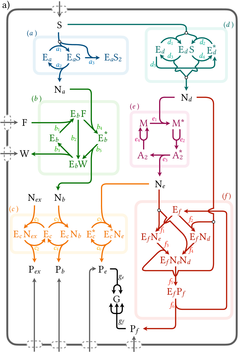
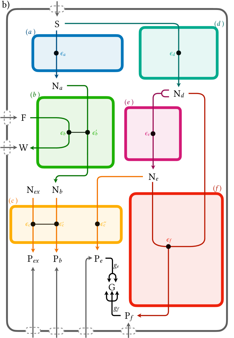
Figure 1: Elementary (a) and circuit description (b) of a complex CRN enclosed in gray boundaries using hypergraph notation. Gray arrows crossing the network boundaries denote the exchange processes with the environment. Colored boxes are chemical modules. Their internal species and (elementary or effective) reactions are represented by chemical symbols and arrows of the same color, respectively. Their terminal species are represented by black chemical symbols. All the chemical reactions are assumed to be reversible even though only the forward reactions are represented. Effective reactions are coupled when connected by black lines.

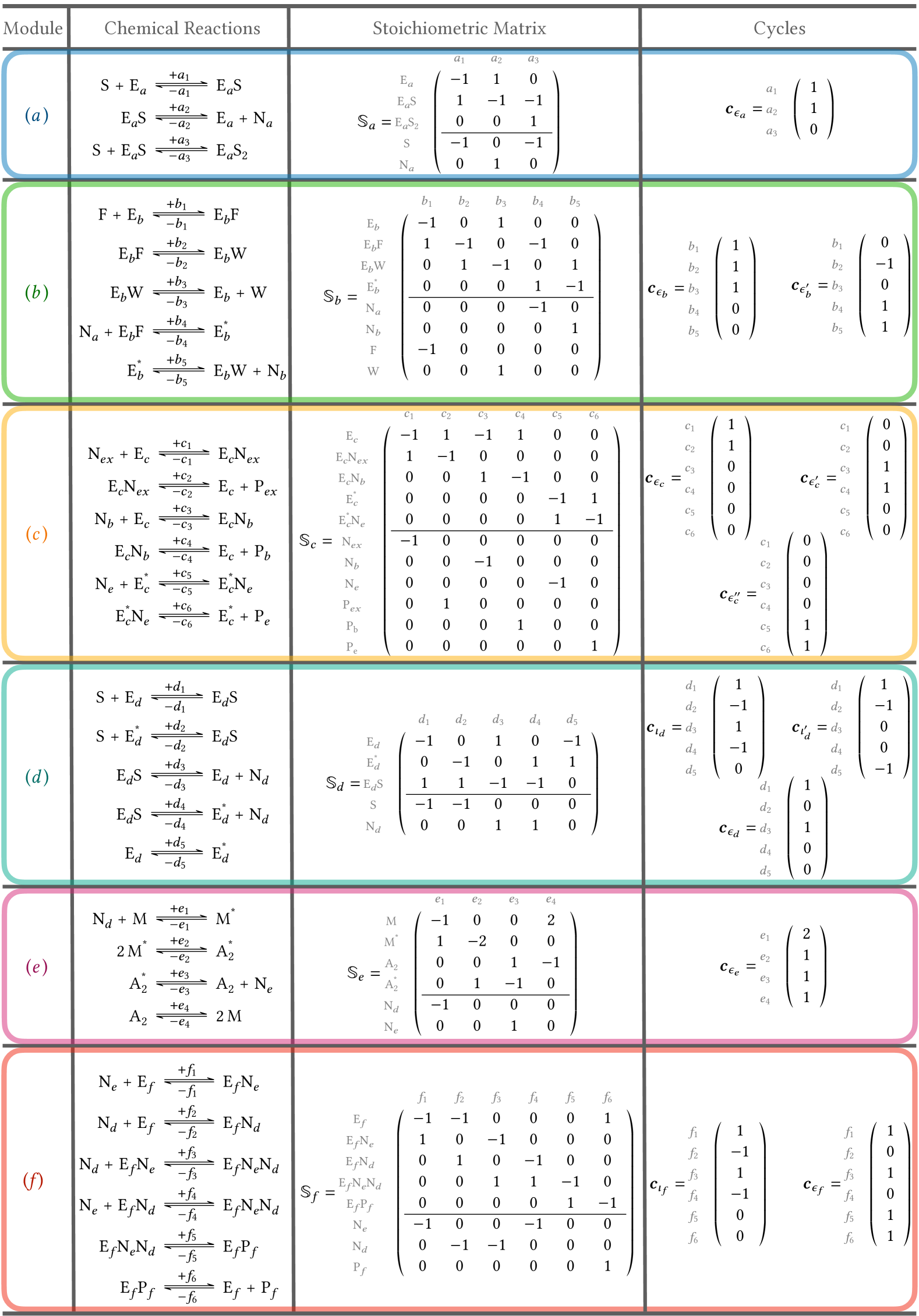
Figure 2: Chemical reactions, stoichiometric matrix, and cycles of the modules in Fig. 1a. The black horizontal line splits the stoichiometric matrix of each module ${\mathbb{S}}{}_{m}$ into the substoichiometric matrix for the internal species ${\mathbb{S}}{}^{Q}_{m}$ and for the terminal species ${\mathbb{S}}{}^{P}_{m}$.

To explain how to reduce the description of a complex open CRN in terms of chemical modules, we will use the CRN depicted in Fig. 1a and reduce it to Fig. 1b. The formal description of this procedure is given in App. LABEL:app:def_chem_module. In particular, App. LABEL:app:def_chem_module_el gives a formal definition of modules, while in Apps. LABEL:app:def_chem_module_eff and LABEL:app:def_chem_module_eff_oscillations their reduced description is derived.

In Fig. 1a, the arrows denote both the chemical reactions of the network as well as the exchange processes with the environment. The latter are represented by (gray) arrows entering the CRN from the outside and involve the exchanged species ($\ch{S}$, $\ch{F}$, $\ch{W}$, $\ch{P_{$ex$}}$, $\ch{P_{$b$}}$, $\ch{P_{$e$}}$, and $\ch{P_{$f$}}$). The direction of the arrows is arbitrary (set by convention) as all reactions are assumed to be reversible. The boxes inside the CRN in Fig. 1a are the modules. Each module is a subnetwork composed of a unique set of internal species (drawn inside the module) reacting among themselves and potentially also with other species, named terminal species (drawn outside the module). For instance, the (blue) module $a$ in Fig. 1a interconverts the internal species $\ch{E_{$a$}}\,,\text{ }\ch{E_{$a$}S}\,,\text{ }\ch{E_{$a$}S_{2}}$ and the terminal species $\ch{S}\text{ }\text{ and }\text{ }\ch{N_{$a$}}$ via the chemical reactions

$$\begin{split}\ch{S+E_{$a$}&<=>[$+a_{1}$][$-a_{1}$]E_{$a$}S}\\ \ch{E_{$a$}S&<=>[$+a_{2}$][$-a_{2}$]E_{$a$}+N_{$a$}}\\ \ch{E_{$a$}S+S&<=>[$+a_{3}$][$-a_{3}$]E_{$a$}S_{2}}\end{split}$$ (1)

represented by the (blue) arrows labeled $a_{1}$, $a_{2}$, and $a_{3}$ (also specified in Fig. 2).

Chemical modules are the chemical analog of the electronic components (for example diodes, transistors, or microchips) of an electric circuit, and the terminal species are the analog of the electrical contacts or pins of each component. Arrows in Fig. 1a should however not be compared to cables or connections between components in an electronic circuit diagram. Instead, the analog of electrical connections between contacts of different electronic components is the chemical species shared between chemical modules, i.e., the terminal species. But while electronic components are spatially separated, chemical modules do not have to be. Assuming homogeneous solutions for simplicity, the definition of the modules as well as their representation is based on the network of reactions and does not require any spatial organization. Situations involving spatial organization will be discussed in Sec. LABEL:sec:discussion.

In the circuit description depicted in Fig. 1b, each module ends up being coarse grained into effective reactions (denoted by the arrows through the boxes) between its terminal species. The coarse graining reduces the (blue) module $a$ to the single effective reaction

$$\ch{S<=>[{\epsilon}_{a}][]N_{a}}\,.$$ (2)

The coarse-graining procedure is based on the stoichiometry of the module and starts from its stoichiometric matrix Palsson2011

$${{\mathbb{S}}{}_{a}}=\hbox{}\vbox{\kern 0.86108pt\hbox{$\kern 0.0pt\kern 2.5pt\kern-5.0pt\left(\kern 0.0pt\kern-2.5pt\kern-6.66669pt\vbox{\kern-0.86108pt\vbox{\vbox{ \halign{\kern\arraycolsep\hfil\@arstrut$\kbcolstyle#$\hfil\kern\arraycolsep& \kern\arraycolsep\hfil$\@kbrowstyle#$\ifkbalignright\relax\else\hfil\fi\kern\arraycolsep&& \kern\arraycolsep\hfil$\@kbrowstyle#$\ifkbalignright\relax\else\hfil\fi\kern\arraycolsep\cr 5.0pt\hfil\@arstrut$\scriptstyle$\hfil\kern 5.0pt&5.0pt\hfil$\scriptstyle\color[rgb]{0.50,0.50,0.50}a_{1}$\hfil\kern 5.0pt&5.0pt\hfil$\scriptstyle\color[rgb]{0.50,0.50,0.50}a_{2}$\hfil\kern 5.0pt&5.0pt\hfil$\scriptstyle\color[rgb]{0.50,0.50,0.50}a_{3}$\hfil\kern 5.0pt\crcr\kern 0.86108pt\cr 5.0pt\hfil\@arstrut$\scriptstyle\color[rgb]{0.50,0.50,0.50}\ch{E_{$a$}}$\hfil\kern 5.0pt&5.0pt\hfil$-1$\hfil\kern 5.0pt&5.0pt\hfil$1$\hfil\kern 5.0pt&5.0pt\hfil$0$\hfil\kern 5.0pt\cr 5.0pt\hfil\@arstrut$\scriptstyle\color[rgb]{0.50,0.50,0.50}\ch{E_{$a$}S}$\hfil\kern 5.0pt&5.0pt\hfil$1$\hfil\kern 5.0pt&5.0pt\hfil$-1$\hfil\kern 5.0pt&5.0pt\hfil$-1$\hfil\kern 5.0pt\cr 5.0pt\hfil\@arstrut$\scriptstyle\color[rgb]{0.50,0.50,0.50}\ch{E_{$a$}S_{2}}$\hfil\kern 5.0pt&5.0pt\hfil$0$\hfil\kern 5.0pt&5.0pt\hfil$0$\hfil\kern 5.0pt&5.0pt\hfil$1$\hfil\kern 5.0pt\cr\cline{2-4}\cr 5.0pt\hfil\@arstrut$\scriptstyle\color[rgb]{0.50,0.50,0.50}\ch{S}$\hfil\kern 5.0pt&5.0pt\hfil$-1$\hfil\kern 5.0pt&5.0pt\hfil$0$\hfil\kern 5.0pt&5.0pt\hfil$-1$\hfil\kern 5.0pt\cr 5.0pt\hfil\@arstrut$\scriptstyle\color[rgb]{0.50,0.50,0.50}\ch{N_{$a$}}$\hfil\kern 5.0pt&5.0pt\hfil$0$\hfil\kern 5.0pt&5.0pt\hfil$1$\hfil\kern 5.0pt&5.0pt\hfil$0$\hfil\kern 5.0pt\cr}}}}\right)$}}\blockarray{cc}&\\ \\ \block{c\}\BAmultirow{1cm}}\\ \>\mathbb{S}_{a}^{Q}\\ \\ \block{c\}\BAmultirow{1cm}}\>\mathbb{S}_{a}^{P}\\ \\ \\ ,$$ (3)

also specified in Fig. 2, whose entries have a clear physical meaning: they encode the net variation of the number of molecules of each species (identified by the matrix row) undergoing each reaction (identified by the matrix column) Palsson2011. This matrix is split into the substoichiometric matrices for the internal species ${{\mathbb{S}}{}^{Q}_{a}}$ and for the terminal species ${{\mathbb{S}}{}^{P}_{a}}$. The effective reactions correspond to the emergent cycles of ${{\mathbb{S}}{}_{a}}$, i.e., a set of linearly independent right-null vectors of ${{\mathbb{S}}{}^{Q}_{a}}$ that are not right-null vectors of ${{\mathbb{S}}{}^{P}_{a}}$. As we will see, this set may not be unique. However, for the stoichiometric matrix (3), one only finds the single emergent cycle:

$${{\boldsymbol{c}}_{{\epsilon}_{a}}}=\hbox{}\vbox{\kern 0.86108pt\hbox{$\kern 0.0pt\kern 2.5pt\kern-5.0pt\left(\kern 0.0pt\kern-2.5pt\kern-6.66669pt\vbox{\kern-0.86108pt\vbox{\vbox{ \halign{\kern\arraycolsep\hfil\@arstrut$\kbcolstyle#$\hfil\kern\arraycolsep& \kern\arraycolsep\hfil$\@kbrowstyle#$\ifkbalignright\relax\else\hfil\fi\kern\arraycolsep&& \kern\arraycolsep\hfil$\@kbrowstyle#$\ifkbalignright\relax\else\hfil\fi\kern\arraycolsep\cr 5.0pt\hfil\@arstrut$\scriptstyle$\hfil\kern 5.0pt&5.0pt\hfil$\scriptstyle$\hfil\kern 5.0pt\crcr\kern 0.86108pt\cr 5.0pt\hfil\@arstrut$\scriptstyle\color[rgb]{0.50,0.50,0.50}a_{1}$\hfil\kern 5.0pt&5.0pt\hfil$1$\hfil\kern 5.0pt\cr 5.0pt\hfil\@arstrut$\scriptstyle\color[rgb]{0.50,0.50,0.50}a_{2}$\hfil\kern 5.0pt&5.0pt\hfil$1$\hfil\kern 5.0pt\cr 5.0pt\hfil\@arstrut$\scriptstyle\color[rgb]{0.50,0.50,0.50}a_{3}$\hfil\kern 5.0pt&5.0pt\hfil$0$\hfil\kern 5.0pt\cr}}}}\right)$}}\,,$$ (4)

also reported in Fig. 2. The sequence of reactions encoded in the emergent cycle interconverts (upon completion) only the terminal species while leaving the internal species unaltered. By multiplying the substoichiometry matrix for the terminal species ${{\mathbb{S}}{}^{P}_{a}}$ in (3) and the emergent cycle ${{\boldsymbol{c}}_{{\epsilon}_{a}}}$ in (4), one obtains the variation of the number of molecules of terminal species along the emergent cycle, i.e., the stoichiometry of the corresponding effective reaction (2):

$${{\mathbb{S}}{}^{P}_{a}}{{\boldsymbol{c}}_{{\epsilon}_{a}}}=\hbox{}\vbox{\kern 0.86108pt\hbox{$\kern 0.0pt\kern 2.5pt\kern-5.0pt\left(\kern 0.0pt\kern-2.5pt\kern-6.66669pt\vbox{\kern-0.86108pt\vbox{\vbox{ \halign{\kern\arraycolsep\hfil\@arstrut$\kbcolstyle#$\hfil\kern\arraycolsep& \kern\arraycolsep\hfil$\@kbrowstyle#$\ifkbalignright\relax\else\hfil\fi\kern\arraycolsep&& \kern\arraycolsep\hfil$\@kbrowstyle#$\ifkbalignright\relax\else\hfil\fi\kern\arraycolsep\cr 5.0pt\hfil\@arstrut$\scriptstyle$\hfil\kern 5.0pt&5.0pt\hfil$\scriptstyle\color[rgb]{0.50,0.50,0.50}$\hfil\kern 5.0pt\crcr\kern 0.86108pt\cr 5.0pt\hfil\@arstrut$\scriptstyle\color[rgb]{0.50,0.50,0.50}\ch{S}$\hfil\kern 5.0pt&5.0pt\hfil$-1$\hfil\kern 5.0pt\cr 5.0pt\hfil\@arstrut$\scriptstyle\color[rgb]{0.50,0.50,0.50}\ch{N_{$a$}}$\hfil\kern 5.0pt&5.0pt\hfil$1$\hfil\kern 5.0pt\cr}}}}\right)$}}\,.$$ (5)

The general and formal discussion of the coarse-grained procedure based on the use of the emergent cycles is given in App. LABEL:app:def_chem_module_eff and App. LABEL:app:def_chem_module_eff_oscillations.

We now turn to the (green) module $b$, whose internal species E_$b$, E_$b$F, E_$b$W, and E_$b$^* react via the chemical reactions $b_{1}$, $b_{2}$, $b_{3}$, $b_{4}$, and $b_{5}$ (see Fig. 2) with the terminal species N_$a$, N_$b$, F, and W. From the corresponding stoichiometric matrix ${\mathbb{S}}{}_{b}$ (in Fig. 2), we identify two emergent cycles ${{\boldsymbol{c}}_{{\epsilon}_{b}}}$ and ${{\boldsymbol{c}}_{{\epsilon}_{b}^{\prime}}}$ (in Fig. 2) which correspond to the following effective reactions between the terminal species

respectively. Note that

$${{\boldsymbol{c}}_{{\epsilon}_{b}^{\prime\prime}}}=\hbox{}\vbox{\kern 0.86108pt\hbox{$\kern 0.0pt\kern 2.5pt\kern-5.0pt\left(\kern 0.0pt\kern-2.5pt\kern-6.66669pt\vbox{\kern-0.86108pt\vbox{\vbox{ \halign{\kern\arraycolsep\hfil\@arstrut$\kbcolstyle#$\hfil\kern\arraycolsep& \kern\arraycolsep\hfil$\@kbrowstyle#$\ifkbalignright\relax\else\hfil\fi\kern\arraycolsep&& \kern\arraycolsep\hfil$\@kbrowstyle#$\ifkbalignright\relax\else\hfil\fi\kern\arraycolsep\cr 5.0pt\hfil\@arstrut$\scriptstyle$\hfil\kern 5.0pt&5.0pt\hfil$\scriptstyle$\hfil\kern 5.0pt\crcr\kern 0.86108pt\cr 5.0pt\hfil\@arstrut$\scriptstyle\color[rgb]{0.50,0.50,0.50}b_{1}$\hfil\kern 5.0pt&5.0pt\hfil$1$\hfil\kern 5.0pt\cr 5.0pt\hfil\@arstrut$\scriptstyle\color[rgb]{0.50,0.50,0.50}b_{2}$\hfil\kern 5.0pt&5.0pt\hfil$0$\hfil\kern 5.0pt\cr 5.0pt\hfil\@arstrut$\scriptstyle\color[rgb]{0.50,0.50,0.50}b_{3}$\hfil\kern 5.0pt&5.0pt\hfil$1$\hfil\kern 5.0pt\cr 5.0pt\hfil\@arstrut$\scriptstyle\color[rgb]{0.50,0.50,0.50}b_{4}$\hfil\kern 5.0pt&5.0pt\hfil$1$\hfil\kern 5.0pt\cr 5.0pt\hfil\@arstrut$\scriptstyle\color[rgb]{0.50,0.50,0.50}b_{5}$\hfil\kern 5.0pt&5.0pt\hfil$1$\hfil\kern 5.0pt\cr}}}}\right)$}}$$ (6m)

is also a right-null vector of ${\mathbb{S}}{}^{Q}_{b}$, which corresponds to the effective reaction

$$\ch{F+N_{a}<=>[{\epsilon}_{b}^{\prime\prime}][]N_{b}+W}\,.$$ (6n)

But it is linearly dependent on the other two and is thus excluded from the circuit description. Any other pair of these three emergent cycles could also have been chosen.

We consider now the (aqua green) module $d$ whose internal species E_$d$, E_$d$^*, and E_$d$S are involved in the chemical reactions $d_{1}$, $d_{2}$, $d_{3}$, $d_{4}$, and $d_{5}$ (see Fig. 2) with the terminal species S and N_$d$. Its stoichiometric matrix is specified in Fig. 2 and, unlike the previous modules, the substoichiometry matrix for the internal species ${{\mathbb{S}}{}^{Q}_{d}}$ admits the right-null vectors ${{\boldsymbol{c}}_{{\iota}_{d}}}$ and ${{\boldsymbol{c}}_{{\iota}_{d^{\prime}}}}$, called internal cycles, that are also right-null vectors of the substoichiometry matrix for the terminal species ${{\mathbb{S}}{}^{P}_{d}}$. These internal cycles are sequences of reactions that upon completion leave all the species (both internal and terminal) unaltered. Thus, they do not correspond to any effective reaction between terminal species. However, the substoichiometry matrix for the internal species admits also the emergent cycle ${{\boldsymbol{c}}_{{\epsilon}_{d}}}$ which corresponds to the following effective reaction

$$\ch{S<=>[{\epsilon}_{d}][\end{equation}]N_{d}}$$

.

By following the same procedure for the remaining modules, one obtains the following effective reactions

$$\begin{split}\ch{N_{$ex$}&<=>[${\epsilon}_c$][$$]P_{$ex$}}\\ \ch{N_{$b$}&<=>[${\epsilon}_c'$][$$]P_{$b$}}\\ \ch{N_{$e$}&<=>[${\epsilon}_c''$][$$]P_{$e$}}\end{split}$$ (6o)

for the (orange) module $c$;

$$\ch{2N_{d}<=>[{\epsilon}_{e}][\end{equation}]N_{e}}$$

, for the (purple) module $e$; and

$$\ch{N_{d}+N_{e}<=>[{\epsilon}_{f}][\end{equation}]P_{f}}$$

.