On the cosmic evolution of AGN obscuration and the X-ray luminosity function: XMM-Newton and Chandra spectral analysis of the 31.3 deg² Stripe 82X

Abstract

We present X-ray spectral analysis of XMM-Newton and Chandra observations in the 31.3 deg² Stripe-82X (S82X) field. Of the 6181 unique X-ray sources in this field, we analyze a sample of 2937 candidate active galactic nuclei (AGN) with solid redshifts and sufficient counts determined by simulations. Our results show an observed population with median values of spectral index $\Gamma=1.94_{-0.39}^{+0.31}$, column density log$\,N_{\mathrm{H}}/\mathrm{cm}^{-2}=20.7_{-0.5}^{+1.2}$ and intrinsic, de-absorbed, 2-10 keV luminosity log$\,L_{\mathrm{X}}/\mathrm{erg\,\,s}^{-1}=44.0_{-1.0}^{+0.7}$, in the redshift range 0-4. We derive the intrinsic, model-independent, fraction of AGN that are obscured ($22\leq\mathrm{log}\,N_{\mathrm{H}}/\mathrm{cm}^{-2}<24$), finding a significant increase in the obscured AGN fraction with redshift and a decline with increasing luminosity. The average obscured AGN fraction is $57\pm 4\%$ for log$\,L_{\mathrm{X}}/\mathrm{erg\,\,s}^{-1}>43$. This work constrains the AGN obscuration and spectral shape of the still uncertain high-luminosity and high-redshift regimes (log$\,L_{\mathrm{X}}/\mathrm{erg\,\,s}^{-1}>45.5$, $z>3$), where the obscured AGN fraction rises to $64\pm 12\%$. We report a luminosity and density evolution of the X-ray luminosity function, with obscured AGN dominating at all luminosities at $z>2$ and unobscured sources prevailing at log$\,L_{\mathrm{X}}/\mathrm{erg\,\,s}^{-1}>45$ at lower redshifts. Our results agree with the evolutionary models in which the bulk of AGN activity is triggered by gas-rich environments and in a downsizing scenario. Moreover, the black hole accretion density (BHAD) is found to evolve similarly to the star formation rate density, confirming the co-evolution between AGN and host-galaxy, but suggesting different time scales in their growing history. The derived BHAD evolution shows that Compton-thick AGN contribute to the accretion history of AGN as much as all other AGN populations combined.

1 Introduction

Active galactic nuclei (AGN) are the manifestation of gas accretion onto supermassive black holes (SMBHs). During this growth phase, AGN produce powerful radiation detectable across the entire electromagnetic spectrum (Antonucci 1993; Urry & Padovani 1995). The evolution of SMBH growth and its relation to the surrounding environment are still a matter of active study due to the need for unbiased multiwavelength samples with high spectroscopic completeness and large enough volume to reach high luminosities and redshifts. AGN selection at optical-UV wavelengths is biased against obscured sources (i.e., with column densities $\log N_{\rm H}/\mathrm{cm}^{-2}>22$) because the primary emission from accretion is scattered or absorbed by dust and gas along our line of sight, either on small circumnuclear scales or in dense clouds in the host galaxy. In the infrared and optical, AGN can also be diluted by stellar emission from the host galaxy.

For these reasons, X-ray selection is a leading approach for defining nearly unbiased samples (e.g., Brandt & Alexander 2015). In particular, hard X-rays ($E\gtrsim 2$ keV) penetrate even large obscuring column densities, leading to relatively complete AGN samples (e.g., Hickox & Alexander 2018). While in the local Universe these studies are possible with telescopes sensitive at energies above 10 keV, like Swift-BAT and NuSTAR (e.g., Marchesi et al. 2019; LaMassa et al. 2019b; Koss et al. 2022), at higher redshifts the relevant penetrating emission enters the Chandra and XMM-Newton $\sim$0.5-10 keV energy band. This allows us to leverage the extensive amount of data available in both the Chandra and XMM-Newton archives. At the same time, the volume density of AGN drops dramatically at the highest luminosities ($\log L_{\rm X}/\mathrm{erg\,\,s}^{-1}>45$) and redshifts ($z>3$) (e.g., Hasinger 2008, Ueda et al. 2014, hereafter U14, Aird et al. 2015, hereafter A15, Buchner et al. 2015, hereafter B15, Miyaji et al. 2015, and Ananna et al. 2019, hereafter A19), leading deep pencil-beam X-ray surveys to miss the most powerful accretors. According to popular models (e.g., Hopkins & Hernquist 2009; Treister et al. 2012), these sources represent evolutionary key phases where the bulk of the mass is accreted onto the central SMBH. Due to their low space density, large area surveys become crucial to collect them in samples large enough to perform population studies. This is why at present, the census of high-luminosity, high-redshift, and highly obscured sources, as well as their evolution, is still poorly known.

Here we address this gap using the large-volume Stripe 82X survey (S82X, LaMassa et al. 2013a, b, 2016), which covers an area of $\sim$31.3 deg² with XMM-Newton and Chandra observations. While S82X is not the only large area survey observed in hard X-rays (e.g., XMM-XXL, Pierre et al. 2016; CDWFS, Masini et al. 2020) which covers the bright portion of the flux-area plane (see e.g., figure 1 in Nanni et al. 2020), it benefits from unprecedented multiwavelength coverage. S82X was observed from the UV to the radio wavebands, including from facilities no longer available like Spitzer and Herschel (see LaMassa et al. 2016; Ananna et al. 2017 for details on the datasets). While X-ray photons are a powerful tool to uncover and study the black hole activity, supporting information about the AGN and their host galaxies is needed for a reliable analysis. In particular, the rich S82X multiband coverage allows the estimate of both spectroscopic and high-quality photometric redshifts, which are fundamental for X-ray spectral fitting (e.g., Salvato et al. 2009; Ananna et al. 2017; Peca et al. 2021).

In this work we perform a detailed X-ray spectral analysis of the S82X sources, using both XMM-Newton and Chandra data. We build the selection function with respect to parameters like flux and $N_{\rm H}$, and derive the intrinsic $N_{\rm H}$ and $L_{\rm X}$ distributions for the S82X sample. Finally, we determine the X-ray luminosity function (XLF) at different redshifts, in order to measure its evolution and inform population synthesis models in the high luminosity and high redshift regimes.

The paper is organized as follows. In §2 we introduce the S82X datasets used in this work. We present the X-ray spectral analysis procedures in §3 and results in §4. In §5 we discuss the evolution of the fraction of AGN that are obscured and derive the intrinsic distributions. The total, obscured, and unobscured XLFs, and the black hole accretion density are also shown and discussed in this section. In §6 we discuss the implications of this work. §7 summarizes the work. Throughout this paper, we assumed a $\Lambda$CDM cosmology with the fiducial parameters $H_{0}=70$ km s^-1 Mpc^-1, $\Omega_{m}=0.3$, and $\Omega_{\Lambda}=0.7$. Errors are reported at the 90% confidence level if not specified otherwise.

2 Data

S82X comprises XMM-Newton and Chandra observations from both proprietary (XMM AO10 and AO13, LaMassa et al. 2013b, 2016) and archival (LaMassa et al. 2013a, 2016) data for a total, non-overlapping area of $\sim$31.3 deg² (Fig. 1). The limiting fluxes are $8.7\times 10^{-16}$, $4.7\times 10^{-15}$, and $2.1\times 10^{-15}$ erg s^-1 cm^-2 in the soft (0.5-2 keV), hard (2-10 keV), and full (0.5-10 keV) bands, respectively (LaMassa et al. 2016, hereafter L16). The broad band is 0.5–10 keV for XMM-Newton observations and 0.5–7 keV for Chandra observations. Table 1 summarizes the number of observations, covered areas, exposure times and number of sources. A detailed description of the XMM-Newton campaign strategy, data reduction and analysis are given by LaMassa et al. (2013a, b), and L16. The most recent version of the master catalog contains 6181 X-ray unique sources (LaMassa et al. 2019a). Of these, 5150 ($\sim 83\%$), 1520 ($\sim 25\%$), and 5628 ($\sim 91\%$) were detected in the soft, hard and full bands, respectively, with a detection significance of $>5\sigma$ for XMM-Newton, and $>4.5\sigma$ for Chandra. The total number of sources with redshift estimates is 5975 ($\sim 97\%$), of which 3375 have spectroscopic redshifts (L16, LaMassa et al. 2019a) and 5972 have photometric redshifts (Ananna et al., 2017). Multiwavelength counterpart matching was performed by running a maximum likelihood algorithm as discussed by L16 and Ananna et al. (2017).

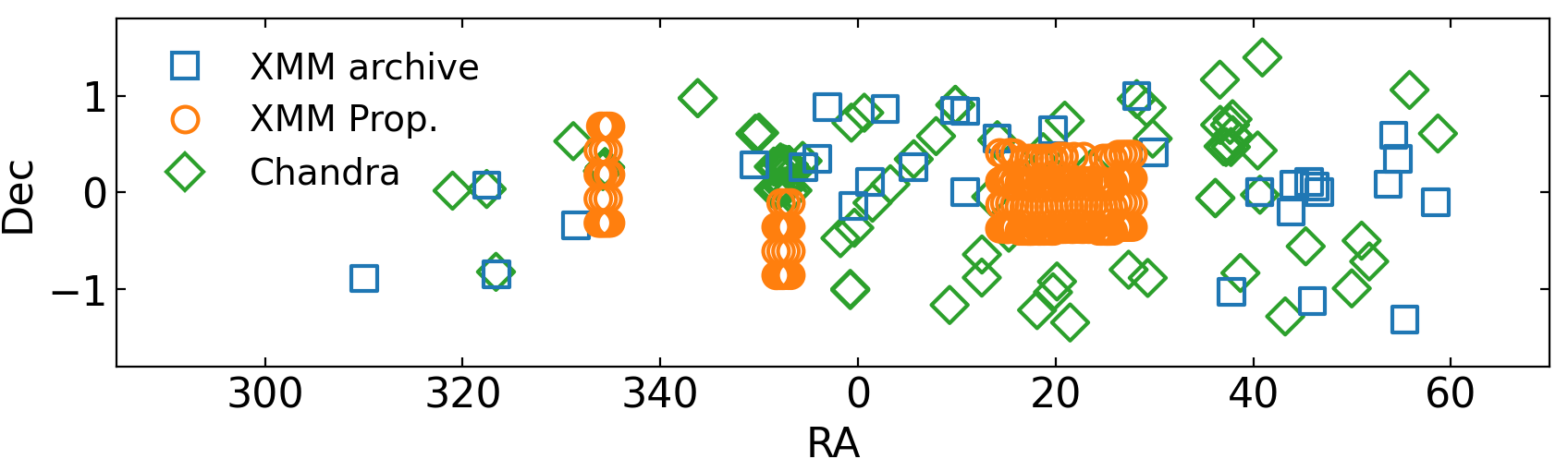
Figure 1: Stripe 82X coverage analyzed in this work: blue squares and orange circles represent XMM-Newton archival and proprietary (AO10 and AO13) observations, respectively; while green diamonds represent Chandra archival data.

Table 1: Stripe 82X Observations

Dataset	Obs	Area	Exp	Srcs
-	-	(deg2)	(ks)	-
Chandra archive	92	7.4	1842	969
XMM archive	33	6.0	775	1599
XMM AO10	2 (44)	4.6	240	751
XMM AO13	7 (154)	15.6	980	2862
Total	134 (323)	33.6 (31.3)	3837	6181

3 X-ray analysis

3.1 Spectral extraction

The spectral extraction was performed with XMM-Newton Standard Analysis System v1.3 (SAS, Gabriel et al. 2004) and Chandra Interactive Analysis of Observations (CIAO, Fruscione et al. 2006) v4.11, for XMM-Newton and Chandra data, respectively. The overall procedure for the spectral extraction is the same for both telescopes. For each source, we defined circular extraction regions by optimizing the signal-to-noise ratio (SNR), using a procedure similar to the SAS task eregionalyse (e.g., Ranalli et al. 2013; Peca et al. 2021). A testing radius centered on the source centroid is varied until the maximum SNR is obtained. The SNR is computed as

$$SNR=\frac{S}{\sqrt{S+BA}},$$ (1)

where $S$ is the number of source counts from the varying source region, $B$ is the background counts from the corresponding background region, and $A$ is the ratio between the source and background areas. To avoid extremely small radii, we set a minimum radius of 16″ or 0.5″, corresponding to the half-light widths at $E=1.5$ keV of the XMM-Newton EPIC camera or the Chandra ACIS camera, respectively. There was no need to set a maximum radius since all the values were within or equal to the 90% encircled energy radius for both telescopes. The background regions were defined as annuli around the sources or—in source-crowded areas or in the case of sources near CCD gaps or edges—as circles close to the corresponding sources. Background regions were defined to be 10 to 100 times larger than the corresponding source regions, and to avoid overlapping the source regions (considering the 90% encircled energy at the source position). Both the source and background spectra were binned to a minimum of 1 count bin^-1 with the grppha tool.

3.2 Background handling

The S82X observations are not deep enough (see Table 1) to allow a good background sampling in local regions close to each source. Specifically, in our sample, there is not a minimum of one background count per spectral channel, which is required to apply a standard background subtraction technique (see Appendix B of the XSPEC manual). We instead decided to model the background and employ the c-stat statistics (Cash, 1979) to deal with the low number of counts. In order to extract a spectrum with enough statistics suitable to model the background, we proceeded as follows. For XMM-Newton, we selected one of the deepest observations in AO13 (0747440101), which is composed of 22 pointings with an average exposure time of $\sim$5 ks each. The detected sources in L16 were removed from the observations considering circular regions with radii corresponding to the 90% of the encircled energy (at 1.5 keV) at the source position. The background spectra were then extracted from each pointing in circular regions of radii 12$\arcmin$ centered at the aimpoint, and combined together with the SAS epicspeccombine tool. This procedure was repeated for the three PN, MOS1, and MOS2 cameras. For Chandra the procedure was similar. The selected deepest observations were 2252 ($\sim$71 ks) for ACIS-I, and 7241 ($\sim$49 ks) and 344 ($\sim$47 ks) for ACIS-S. We used a radius of 8$\arcmin$ for Chandra ACIS-I, while for Chandra ACIS-S we combined the spectra extracted from each of the six CCDs, with a radius of 4$\arcmin$. The stacking procedure was done with the CIAO combine_spectra tool. The final background spectra have a number of counts between 50,000 and 150,000. They were modeled as described in Appendix A, and the best-fit model was used to fit the local background for each source, leaving the background normalization free to account for possible local variations (e.g., Lanzuisi et al. 2013). The spectral fitting was performed using XSPEC v12.10.1 (Arnaud, 1996) through the PyXspec package. Source and background spectra were fitted simultaneously.

3.3 Spectral Models

We fitted the spectra of each source using one or more of the models described below, based on their number of counts (see Section 3.3.1). Ordered from the simplest to the most complex:

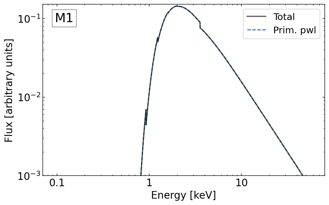
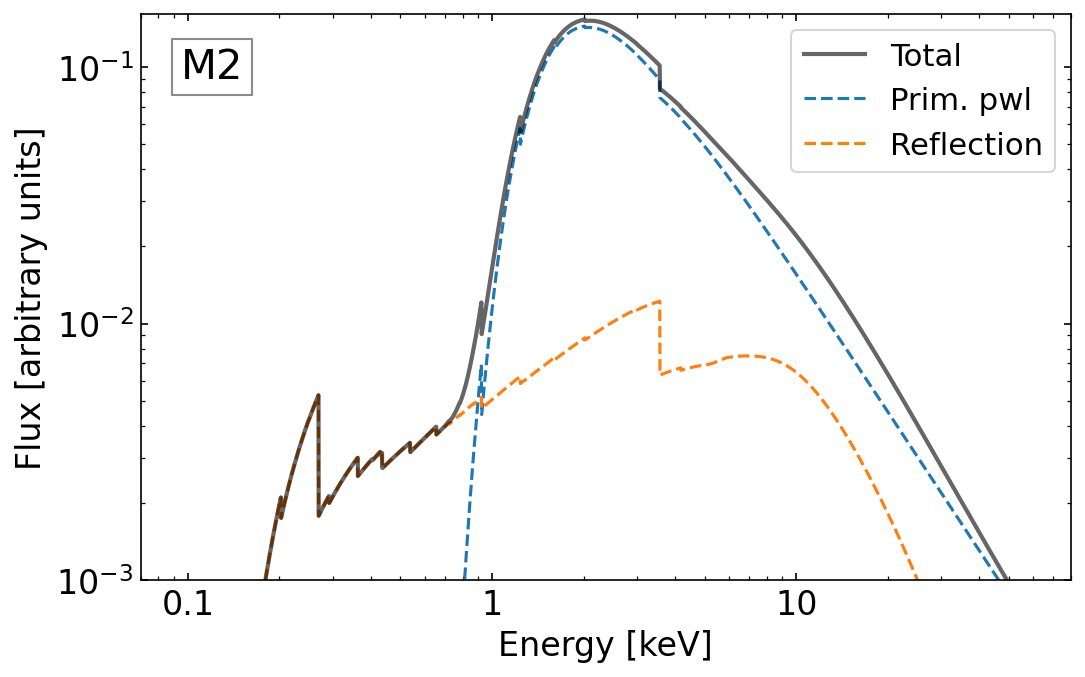
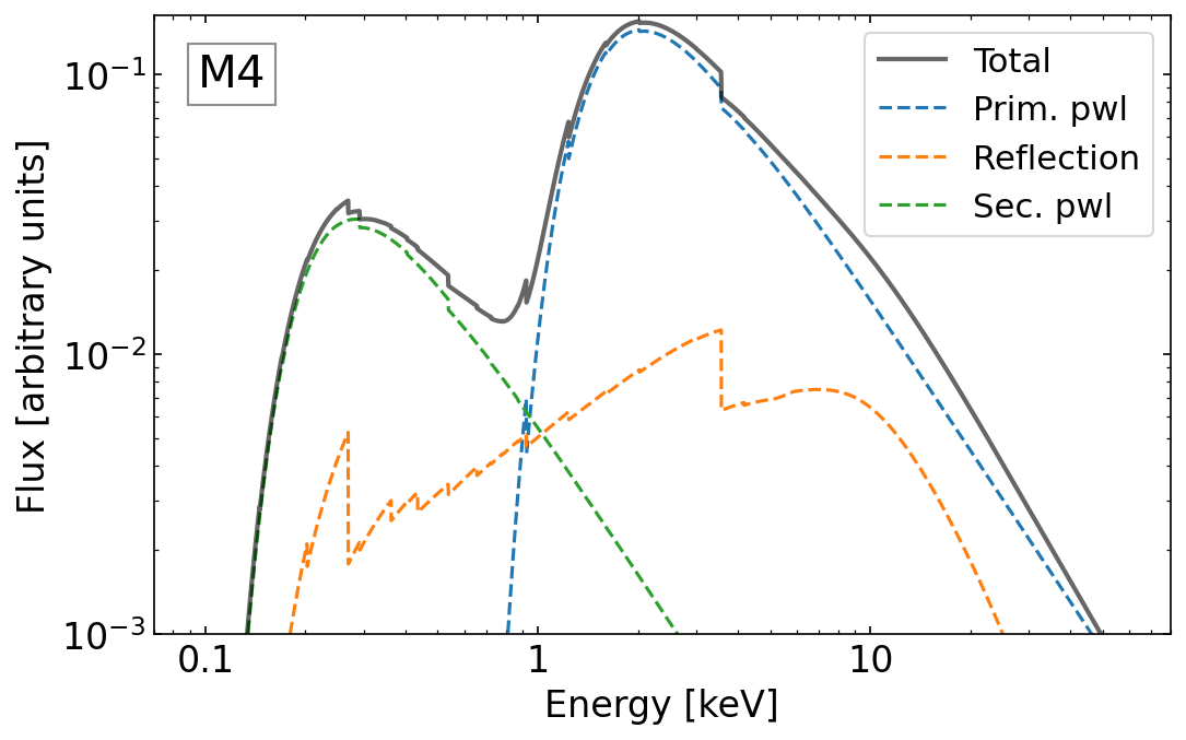
Figure 2: The four models used in the spectral analysis. M1: single absorbed power-law, M2: single absorbed power-law plus reflection, M3: double power-law model, and M4: double power-law model plus reflection. For this figure, the values $z=1$, $N_{\rm H}=10^{23}$ cm² and $\Gamma=1.9$ were assumed; Galactic absorption of 2$\times 10^{20}$ cm^-2 was applied; and the normalization of the secondary power-law was fixed at 2% of the primary power-law. Dashed lines represent the main power-law (blue), reflection (orange), and secondary power-law (green) component; while the black solid lines show the total model. See text for model details.

• M1: Single absorbed power-law (XSPEC model zphabs $\times$ cabs $\times$ zpowerlw): We modeled the effects of absorption on the primary X-ray emission (zpowerlw) by considering photoelectric absorption (zphabs) and Compton scattering (cabs). In particular, the latter is relevant for $\log N_{\rm H}/\mathrm{cm}^{-2}>22.5$ (e.g., Suchy et al. 2012), where part of the radiation is scattered out of the line of sight. The only parameter of the cabs component is the absorption $N_{\rm H}$, which was linked to the zphabs component. Even if its shape might not be the best description of the X-ray spectral shape (e.g., Murphy & Yaqoob 2009), the single power-law is a standard in the literature (e.g., Iwasawa et al. 2012; Marchesi et al. 2016). Especially in the case of low photon statistics, where the use of many free parameters is not justified, the simple power-law is an effective model for comparing general physical properties such as $N_{\rm H}$ and $L_{\rm X}$ among AGN (e.g., Iwasawa et al. 2020). The free parameters for this model are then normalization, $N_{\rm H}$, and photon-index $\Gamma$.

• M2: Simple absorbed power-law plus reflection (zphabs $\times$ cabs $\times$ zpowerlw + pexrav): The reflection component, produced by the reprocessing of the primary X-ray continuum by circumnuclear material, was introduced adding the pexrav model (Magdziarz & Zdziarski 1995) to M1. In pexrav, both the photon index and the normalization were linked to the primary power-law. The reflection parameter $R$ was fixed to 1: since $R=\Omega/2\pi$, where $\Omega$ is the solid angle of the cold material visible from the hot corona, $R=1$ means the reflection is caused by an infinite slab illuminated by the isotropic corona emission. The other parameters were set to their default values. Due to the geometrical assumptions, pexrav can be considered a simplistic model (e.g., Yaqoob 2012; LaMassa et al. 2014; Baloković et al. 2021), but it is widely used (e.g., Buchner et al. 2014; Ricci et al. 2017a), especially in case of low photon statistics (e.g., Lanzuisi et al. 2013). The free parameters for this model are the same of M1.

• M3: Double absorbed power-law (zphabs $\times$ cabs $\times$ zpowerlw + const $\times$ zpowerlw): A second unabsorbed power-law was added to M1, in order to cover a possible soft-excess below $\sim$1-2 keV. It can be produced by different mechanisms, including scattered X-ray photons in circumnuclear material (e.g., Ueda et al. 2007), emission of thermal plasma due to star formation (e.g., Iwasawa et al. 2011), relativistic reflection (e.g., Vasudevan et al. 2014), Comptonization of optical/UV photons in plasma colder than the one in which X-ray photons originate (e.g, Boissay et al. 2014), or absorption by partially ionized material (e.g, Gierliński & Done 2004). The photon index was linked to the primary power-law, and the normalization was constrained to be $\leq$20% of the primary component, as previously observed in X-ray surveys (e.g., Marchesi et al. 2016; Ricci et al. 2017a). The free parameters for this model are then the two power-law normalizations, $N_{\rm H}$, and photon-index $\Gamma$.

• M4: Double absorbed power-law plus reflection (zphabs $\times$ cabs $\times$ zpowerlw + const $\times$ zpowerlw + pexrav): The reflection component was added to M3, with its parameters tuned as described for M2. The free parameters for this model are the same of M3.

Moreover, for each model:

• The photon index was both left free to vary and fixed to a typical observed $\Gamma=1.8$ (e.g., Nandra & Pounds 1994; Piconcelli et al. 2005).

• A calibration constant (const) was added before each model to consider possible normalization issues between XMM-Newton and Chandra. This term was left free to vary when XMM-Newton and Chandra spectra were fitted simultaneously, otherwise it was set to 1.

• Fixed Galactic absorption (phabs) appropriate to the source position (Kalberla et al. 2005) was included.

• The redshift parameter was frozen to the source redshift. We used spectroscopic redshift ($z_{spec}$) when available, and reliable photometric redshifts ($z_{phot}$) otherwise. We defined reliable $z_{phot}$ those redshifts with PDZ$\geq 70\%$, where PDZ is defined as the probability that the true redshift is within $\pm 0.1(1+z_{phot})$ of $z_{phot}$ (see Ananna et al. (2017) for details).

One may think that such simple models do not adequately reproduce the complex shape of the AGN spectrum. However, more sophisticated and physically motivated models, such as MYTORUS (Murphy & Yaqoob 2009) or borus02 (Baloković et al. 2018), require many more photons to be used effectively (e.g., LaMassa et al. 2014; Marchesi et al. 2019; LaMassa et al. 2019b). Our sample has a median value of 38.5 net counts. With such low count statistics, parameters of sophisticated models need to be frozen to standard values to avoid possible degeneracies. As a consequence, their shape becomes similar to our models and produces consistent results (e.g., Brightman et al. 2014). It is worth mentioning that this is true for low obscuration levels up to $\log N_{\rm H}/\mathrm{cm}^{-2}\sim 24$ (e.g., Marchesi et al. 2020), which is what we found in our sample as shown in Section 4. Moreover, overly complex spectral shapes may lead to worse spectral fits: fluctuations in the spectrum, which are very common for low counts sources, may be misinterpreted by XSPEC as spectral features (Peca et al. 2021) causing inaccurate results. For these reasons, it makes more sense to use simple models in the case of low count statistics, when deriving main physical properties like $N_{\rm H}$ and $L_{\rm X}$. For completeness, we show a comparison between our results and the borus02 model in Section 4.2.

3.3.1 Counts threshold evaluation

The average photon statistics in the S82X requires an investigation of the minimum number of counts needed to obtain a reliable fit. We evaluated the fit performance with XSPEC spectral simulations. For each model, we simulated spectra with typical AGN parameters: $\log N_{\rm H}/\rm{cm}^{-2}$ from 20 to 24.5 in logarithmic bins of 0.5, redshift from 0 to 5 in unitary bins, a fixed $\Gamma=1.8$, and a variable normalization in order to obtain a range of net counts between 0 and 100. For each parameter combination, 1000 spectra were simulated. We fitted the simulated spectra applying the same procedure described in 3.2. To check the fit reliability as function of the simulated parameters (counts, $z$, $N_{\rm H}$), we computed the match percentage (Peca et al. 2021):

$$\mathrm{MP}({\mathrm{c}ts},z,N_{\rm H},\Gamma)=\frac{N(X\pm\Delta X)}{N_{\rm sim}}(X).$$ (2)

This is the fraction of simulated spectra for which the fitted values of $X$ ($N_{\rm H}$ or $\Gamma$) are consistent with the simulated values within a given tolerance $\Delta X$ (90% uncertainty) for specific values of the number of counts, redshift, $N_{\rm H}$, and spectral index. We chose a threshold of MP%$\geq 50\%$. As shown by Peca et al. (2021), this threshold is a fair compromise between having a large enough sample and spectral fit accuracy. Since it is common to find $N_{\rm H}$ upper limits in X-ray surveys (e.g., Marchesi et al. 2016), we considered them as good values, while we rejected $\Gamma$ solutions that were not constrained between boundaries. Because $N_{\rm H}$ values are not known a priori as they are a free variable in the fit, the results were averaged over the $N_{\rm H}$ simulated values. The procedure was then repeated considering $\Gamma$ values in the range 1.6-2.1 (Nandra & Pounds 1994; Piconcelli et al. 2005) with a step of 0.1, but no significant changes in the match percentage were found. In the simulations we used the response matrices from a subset of sources observed at different epochs (XMM-AO13, XMM-AO10, and XMM-Newton and Chandra archives) to consider possible differences due to the effective area degradation during the years. We found a negligible effect on match percentage for bright sources and an overall scatter within $\sim$5% for sources with $\lesssim$50 counts in both the telescopes. We averaged the match percentage obtained for each set of responses for XMM-Newton and Chandra separately.

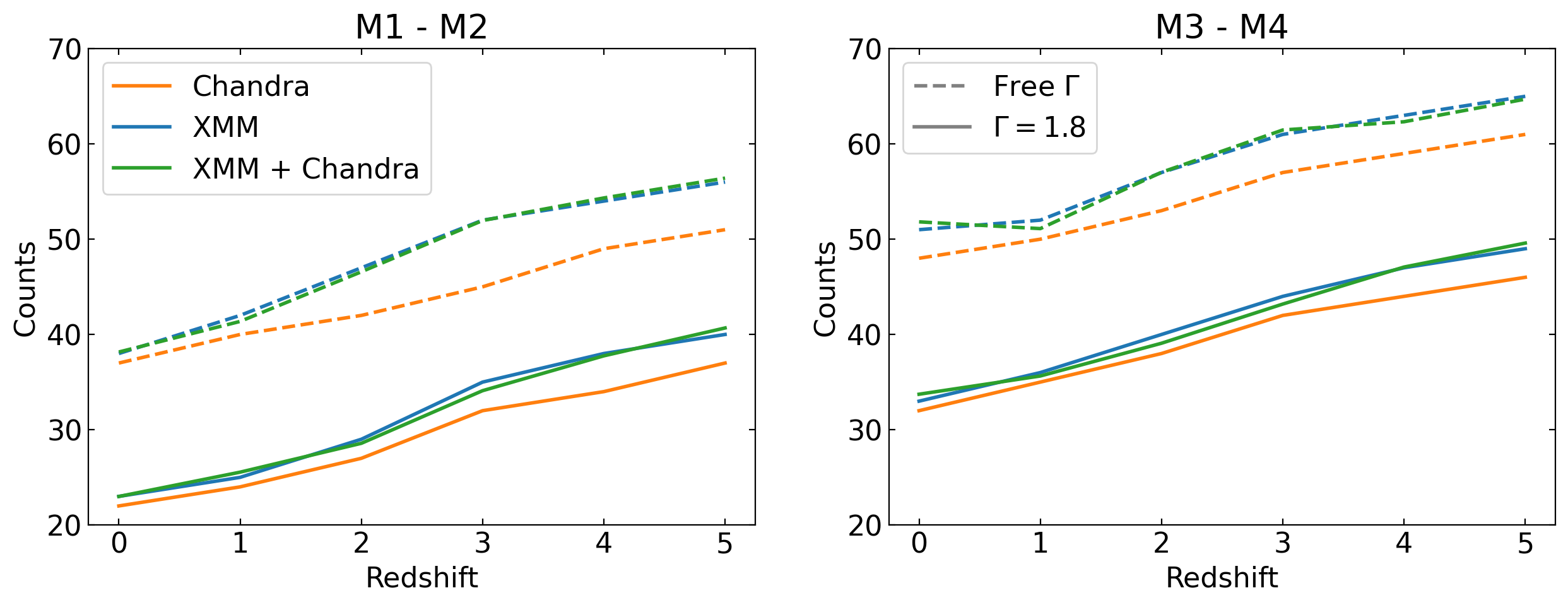
Figure 3: Counts thresholds determined for simple power-law models without and with reflection (M1-M2, respectively; left panel) and double power-law models without and with reflection (M3-M4, respectively; right panel). Blue curves represent values obtained for XMM-Newton data, orange curves are those obtained for Chandra data, and green curves represent XMM-Newton and Chandra together. Solid curves show models where $\Gamma$ was frozen, while dashed curves indicate where $\Gamma$ was free to vary. In the left (right) panel, the curves are valid for both M1 and M2 (M3 and M4) because, even if a reflection component is added, all new parameters are either frozen to standard values or linked to other components.

In Figure 3 we show the results of these simulations for models M1 to M4. As the model complexity increases (and with it the number of parameters), the minimum number of counts required for a reliable fit increases as well. For example, when fitting model M1 with $\Gamma=1.8$ (solid line, left panel), it is possible to get reliable results for sources down to $\sim$20 net counts; while using the same model with a free $\Gamma$ (dashed line, left panel), roughly 35-40 counts are required. The same trends were obtained for model M3 (right panel), but with an increased minimum number of counts due to the more complex spectral shape. For models M2 and M4, we used the same curves obtained for M1 and M3, respectively. In M2 and M4 we introduced a reflection component without new free parameters and, not surprisingly, the results are very similar to those of M1 and M3. Other than the differences in the model complexity, there is also a trend with redshift. This is because as the redshift increases, the AGN spectral shape is shifted to lower energies until part of it lies outside the fitting range, resulting in a lower match percentage and, therefore, in a higher number of minimum counts. This effect is particularly important for obscured sources, whose spectral shape is absorbed in the soft band (e.g., Akylas et al. 2006).

When multi-instrument spectra were available for the same source, we fitted them simultaneously. We were then left with several fitting scenarios: from a single spectrum fitted alone to various XMM-Newton and Chandra spectra fitted together. We opted to perform spectral simulations for the cases that happened most frequently in our sample, namely: i) three XMM-Newton spectra (PN, MOS1, and MOS2), ii) three XMM-Newton spectra plus a single Chandra spectrum, and iii) a single Chandra spectrum only. As shown in Figure 3, the curves found for cases i) and ii) are consistent with each other. For case iii), instead, we found a slight systematic improvement (up to $\sim$7 counts) compared to the other cases. This can be explained because of the different backgrounds in Chandra and XMM-Newton. Having a lower background level, Chandra spectra alone need a slightly lower number of counts to get a reliable fit. We also tested the above cases using both Chandra ACIS-I and ACIS-S spectra, without finding a significant change in the results. Based on the computed curves (Figure 3), we set our count thresholds as a function of $z$, number of counts, and model.

3.4 Model comparison

When more than one model is used to fit a source, a statistical comparison among those models is required to select the best result. Two tests often applied together are the Bayesian Information Criterion (BIC, Schwarz 1978) and the Akaike Information Criterion (AIC, Akaike 1974). Both are valid for nested and non-nested models. In general, due to a different penalization term (see e.g., Kass & Raftery 1995), BIC penalizes more complex models, i.e., with a larger number of parameters, compared to AIC (e.g., Feigelson & Babu 2012; Chakraborty et al. 2021). We therefore decided to apply the AIC test to not penalize the double power-law models, which are more complex but more realistic and physically motivated than the single power-laws (e.g., Lanzuisi et al. 2015; Ricci et al. 2017a).

AIC is defined as

$$AIC=-2\ln(L)+2k,$$ (3)

where $L$ is the maximum likelihood from the fit and $k$ is the number of free parameters. In XSPEC, $L$ can be retrieved from the fit results, as $cstat=-2\times ln(L)$. When the sample size is small, however, the AIC test (as expressed in Eq. 3) may over-fit, selecting models with too many free parameters (e.g., Liddle 2007). This issue can be solved by introducing a correction term in Eq. 3 (e.g., Cavanaugh 1997):

$$AIC_{c}=AIC+\frac{2k(k+1)}{N-k-1},$$ (4)

where $N$ is the number of data points. The AIC criterion states that when there is a set of competing models, the one with the lowest AIC value is preferred. However, it is not the absolute AIC value that is important, but the AIC differences between different models (Burnham & Anderson 2002). In our case, when a source has enough counts to be fitted with a set of models, the AIC differences are computed over the models in the set:

$$\Delta AIC_{c,i}=AIC_{c,i}-AIC_{c,min},$$ (5)

where $AIC_{c,min}$ is the minimum value in the set. If more than one model falls in the range $0\leq\Delta AIC_{c,i}<2$, then the evidence that these models are competitive for being the best model is considered “substantial” (e.g., Burnham & Anderson 2002). When this case is verified, we take the more complex model as the best model since it has more diagnostic power on the physical nature of the AGN.

For completeness, it is worth mentioning that the BIC criterion ($BIC=-2\ln(L)+k\ln(N)$) was also tested. As expected, for the majority (91%) of the sources we obtained the same results of the AIC criterion. For the remaining 9%, the BIC prefers simpler models, but never with a “strong” (i.e., $\Delta BIC>6$, Kass & Raftery 1995) evidence against the more complex models chosen by the AIC. For these cases, the competitive models are then roughly equally consistent with the data, and there is not statistical evidence to strongly favor one over the other, further justifying our choice to pick the more physical motivated one. In this regard, it should be noted that tests such as AIC and BIC compare models from a purely statistical perspective, and thus a physical interpretation in the choice of the best model should also be taken into account.

4 Results

In this section we report the main results derived from the spectral fitting. We narrowed the sample to include only sources with $z_{spec}$, reliable $z_{phot}$ (PDZ$\geq 70\%$), and with enough counts. Spectroscopic classified stars were also removed. The final sample contains 2937 candidate AGN ($\sim 48\%$ of the total sample). Since X-ray sources with $\log L_{\rm X,2\text{-}10keV}/\mathrm{erg\,\,s}^{-1}<42$ may be either low luminosity AGN or non-AGN (e.g., B15, Padovani et al. 2017), we performed the spectral analysis for all the 2937 sources and discussed our results with and without the 185 ($\sim 6\%$) sources with $\log L_{\rm X}/\mathrm{erg\,\,s}^{-1}<42$. The results are released within the catalog described in Appendix B.

4.1 Fit results

In Figure 4 we show the results of model selection described in Section 3.4. Considering the full sample (top panel), around 80% of the sources preferred models without the reflection component (M1 and M3): even if there is the same number of free parameters between models with and without reflection, the $\Delta AIC$ criterion prefers simpler spectral shapes. There is not a significant difference between models with free and frozen $\Gamma$, and single power-law models (M1 and M2) are preferred ($\sim 54\%$) over double power-law models (M3 and M4). However, there is a bias towards simpler models in this pie chart, since spectral models were fitted as a function of the number of counts. Considering, instead, only sources with $>65$ counts (bottom panel), i.e. where all the models were tested according to our count thresholds, we can see that while models without reflection (M1 and M3) are still preferred ($\sim 72\%$), now models with a fixed $\Gamma$ are disfavoured and double power-law models (M3 and M4) are preferred ($\sim 57\%$) over the single power-law models (M1 and M2). In particular, the last trend is confirmed for sources with $>250$ counts, where double power-law models are preferred over single power-law models in $\sim 64\%$ of the cases. We can conclude that, in general, the secondary power-law component becomes statistically more evident as the number of counts increases. In other words, since more complex spectral models have more parameters than simple ones, more counts are needed for them to be statistically chosen as the best representation of observed spectra.

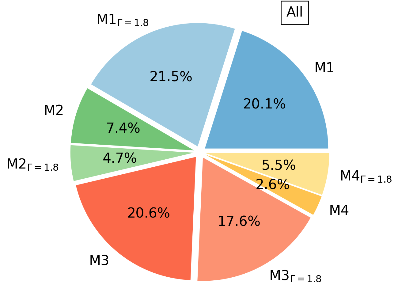
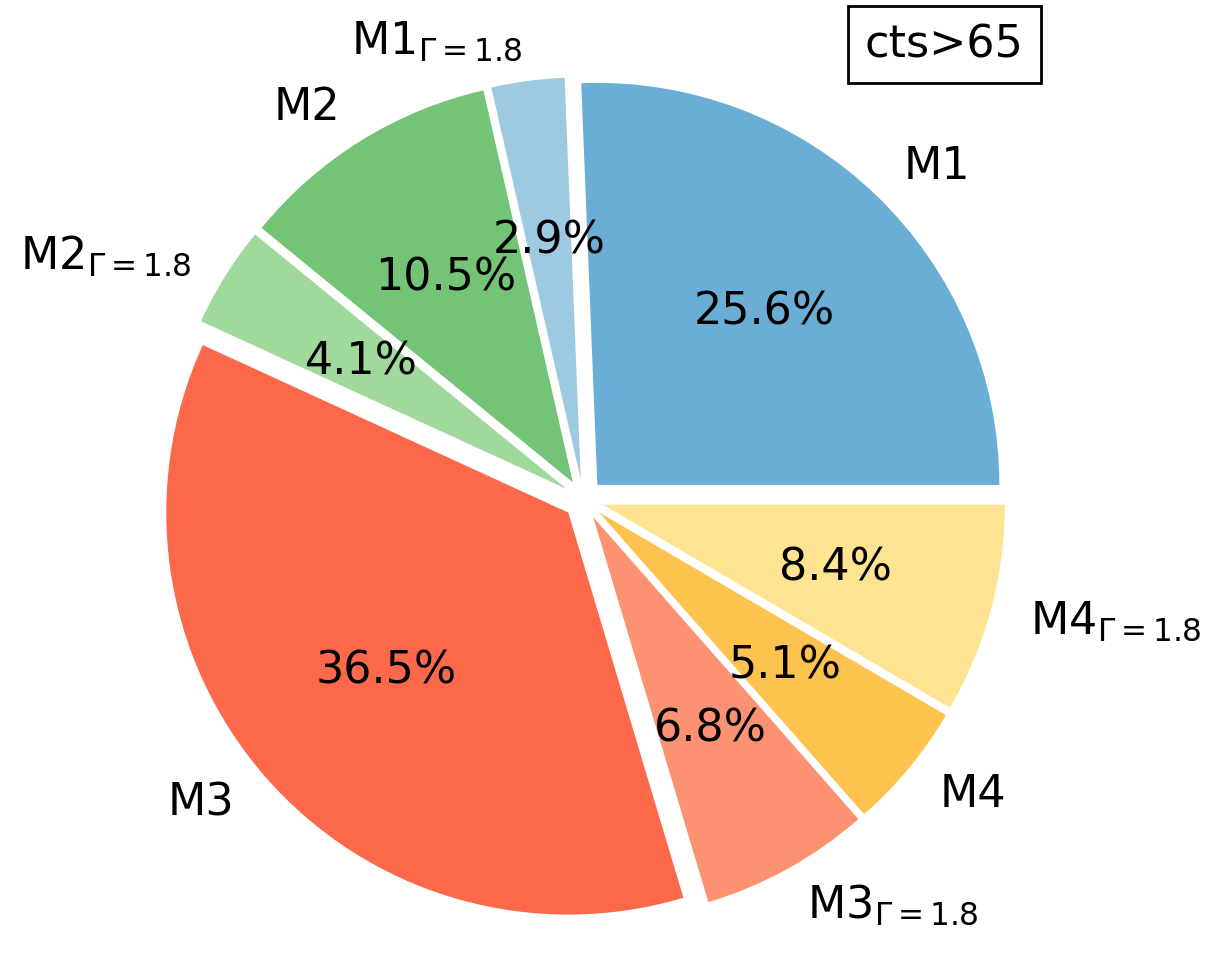
Figure 4: Pie charts of the selected best-fit models for all the sources (top panel) and for sources with net counts $>65$ (bottom panel). For each model we show the results with a free $\Gamma$ (models M1 to M4) and frozen $\Gamma$ (models M1 to M4 with $\Gamma=1.8$ as subscript). Percentages are shown in each pie slice.

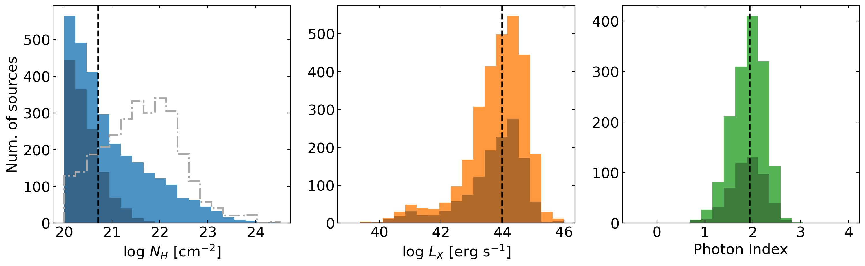
Figure 5: Distributions of key parameters from spectral analysis. Left to right: $N_{\rm H}$ (blue), intrinsic 2-10 keV luminosity (orange), and photon index (green). The grey dash-dotted line in the left panel represents the $N_{\rm H}$ distribution considering upper limits. For each distribution, the median values (see text) are shown with a dashed vertical line. Darker colors indicate sources where the derived $N_{\rm H}$ has only upper limits. In the photon index distribution, all the sources fitted with a fixed $\Gamma=1.8$ were removed.

Figure 5 shows the observed distributions of column density (left panel), X-ray luminosity (absorption-corrected, 2-10 keV, rest-frame; middle panel), and photon index (right panel); whose median values are $\log N_{\rm H}/\mathrm{cm}^{-2}=20.7_{-0.5}^{+1.2}$ ($21.6_{-0.9}^{+0.7}$ considering upper limits), $\log L_{\rm X}/\mathrm{erg\,\,s}^{-1}=44.0_{-1.0}^{+0.7}$, and $\Gamma=1.94_{-0.39}^{+0.31}$, respectively. The uncertainties correspond to the 16^th and 84^th percentiles. These results are consistent with the spectral analysis of the XMM-XXL North field ($\Gamma=1.98_{-0.05}^{+0.09}$, $\log N_{\rm H}/\mathrm{cm}^{-2}=20.9_{-0.3}^{+0.8}$, and $\log L_{\rm X}/\mathrm{erg\,\,s}^{-1}=44.0_{-1.0}^{+0.6}$, by Liu et al. (2016)), which has similar depth and area as S82X. Moreover, we find that 420 ($\sim 14\%$) of the detected S82X AGN are obscured ($\log N_{\rm H}/\mathrm{cm}^{-2}>22$), similarly to the $\sim 12\%$ of XMM-XXL. It is worth noticing that these numbers also agree with those obtained by Mountrichas et al. (2020), which performed a X-ray analysis on infrared selected AGN in S82X. Obscuration and X-ray luminosity distributions vary as a function of depth and covered area (e.g., ; ). Indeed, analyzing the smaller, deeper C-COSMOS field (2.2 deg², 4.6 Ms), Marchesi et al. (2016) found mean $\log L_{\rm X}/\mathrm{erg\,\,s}^{-1}=43.7_{-0.7}^{+0.5}$ and $\log N_{\rm H}/\mathrm{cm}^{-2}=22.7_{-0.5}^{+0.4}$, while in the still smaller and deeper CDF-South field (CDF-S, $\sim 0.11$ deg², 7 Ms), Liu et al. (2017) found median $\log L_{\rm X}/\mathrm{erg\,\,s}^{-1}=43.5_{-0.6}^{+0.7}$ and $\log N_{\rm H}/\mathrm{cm}^{-2}=23.0_{-1.0}^{+0.9}$. As expected, large-volume surveys like S82X or XMM-XXL are more sensitive to luminous, unobscured AGN, while deep pencil-beam surveys detect more obscured and faint objects. Figure 6 shows this concept in the luminosity-redshift plane: while S82X shares the high luminosity region with XMM-XXL, smaller area surveys cover lower luminosity ranges. In particular, CDF-S and C-COSMOS fields combined have only three sources at $\log L_{\rm X}/\mathrm{erg\,\,s}^{-1}>45$ and $z>3$, while S82X and XMM-XXL have 21 and 13 sources, respectively. This strengthens the statement that large area surveys are needed to detect and study high redshift and high luminosity AGN.

Our photon index values are in agreement with many other surveys (e.g., CDF-S, Liu et al. 2017; C-COSMOS, Marchesi et al. 2016; Swift/BAT, Ricci et al. 2017a; J1030, Signorini et al., in prep), suggesting that, on average, the primary power-law slope is not correlated with luminosity or absorption. Figure 7 shows the distribution of the $P_{\rm scatt}$ parameter, which represents the percentage of emission in the secondary power-law (model M3 and M4) compared to the primary component. As discussed before, we observed a significant soft-excess component in $\sim 57\%$ of the sources, in agreement with results from Ricci et al. (2017a) in the local Universe. The median value is $\log P_{\rm scatt}=0.2\pm 0.5$, also consistent with Ricci et al. ($0.1_{-0.7}^{+0.6}$). This consistency suggests that AGN should routinely be fitted with models that include a secondary power-law or other component that account for the soft-excess.

By excluding possible non-AGN sources with $\log L_{\rm X}/\mathrm{erg\,\,s}^{-1}<42$, we found no significant impact on the model selection analysis and consistent median values on the derived physical parameters: $\log N_{\rm H}/\mathrm{cm}^{-2}=20.8_{-0.5}^{+1.2}$ ($21.7_{-0.9}^{+0.7}$ considering upper limits), $\log L_{\rm X}/\mathrm{erg\,\,s}^{-1}=44.1_{-0.8}^{+0.6}$, with no changes for $\Gamma$ and $\log P_{\rm scatt}$.

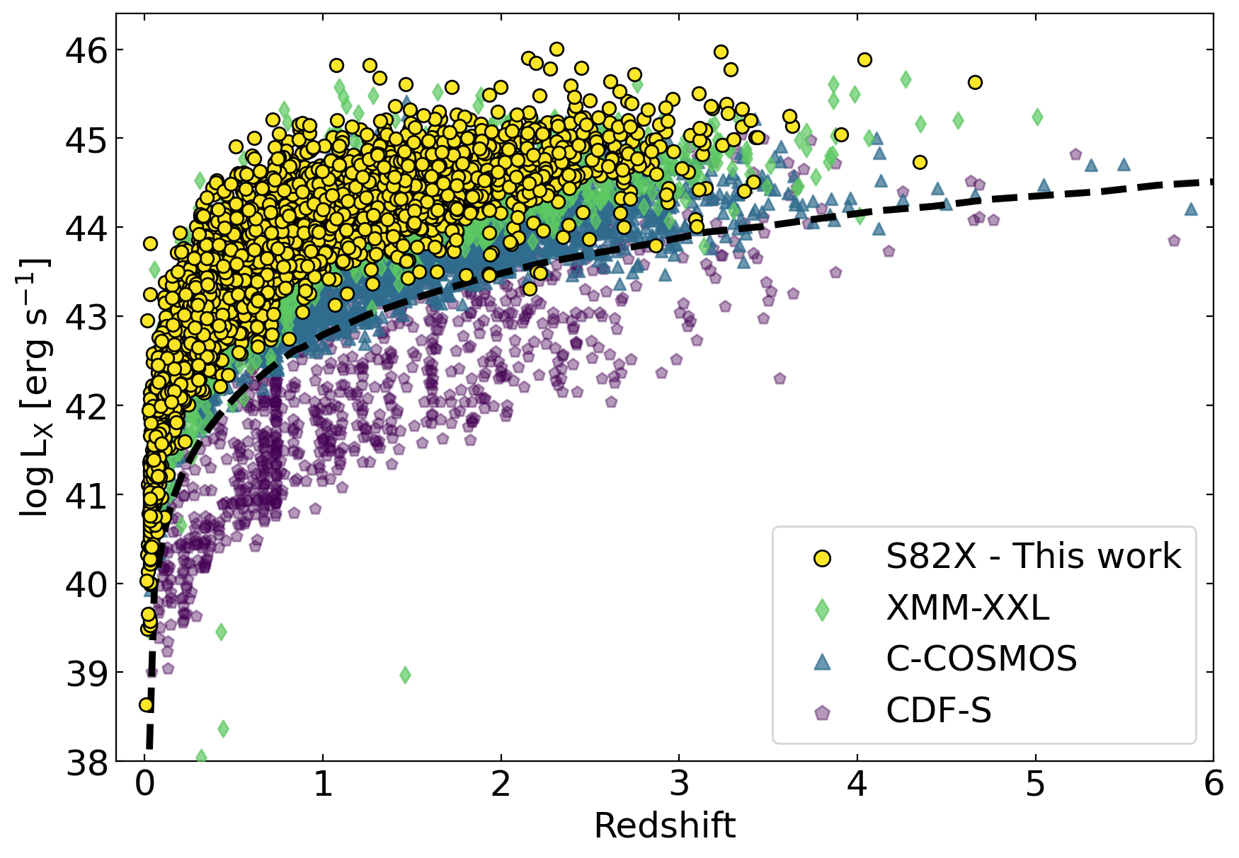
Figure 6: Intrinsic, de-absorbed 2-10 keV luminosity as a function of redshift derived in this work (yellow circles) compared to XMM-XXL (green diamonds; Pierre et al. 2016, Liu et al. 2016), C-COSMOS (blue triangles; Civano et al. 2016, Marchesi et al. 2016), and CDF-S (purple pentagons; Luo et al. 2017, Liu et al. 2017) surveys. The dotted black line represents the S82X survey sensitivity limit from L16.

Figure 7: Distribution of the $P_{\rm scatt}$ parameter, which represents the percentage of emission from the secondary component relative to the primary power-law. The dashed line indicates the median value, $\log P_{\rm scatt}=0.2\pm 0.5$, which indicates that most sources show a significant soft-excess and should be fitted with models that account for it.

4.2 Comparison to a more sophisticated torus model

In this analysis, we used simple models due to the limits set by low photon statistics. While these models allow a reliable parameter estimation, more complex and physically motivated shapes might better describe the actual AGN spectrum and its features. The spectrum of an unobscured AGN is relatively easy to model, since the main power-law component dominates the overall spectral shape. Some features, such as emission lines and/or absorbers of various nature (e.g., Blustin et al. 2005) may be present, but require high photon statistics to be detectable. On the other hand, the spectral shape of obscured AGN is driven by obscuration, and it may be modeled even with a low number of counts (e.g., Iwasawa et al. 2012, 2020; Peca et al. 2021). For these reasons, we tested our results for obscured sources with a more detailed model.

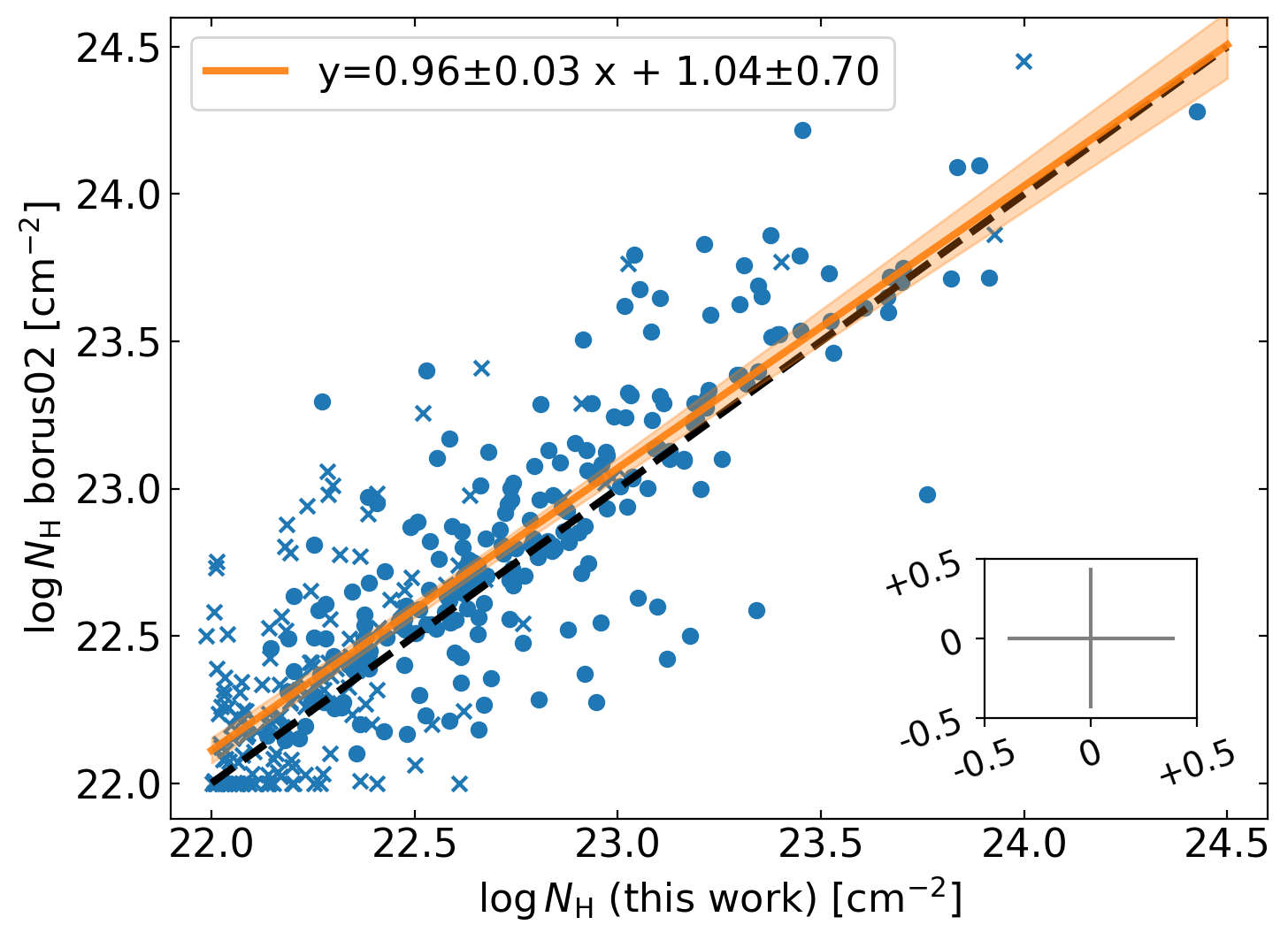
Figure 8: Comparison between log$N_{\rm H}$ values obtained with the borus02 model and models M1 to M4. Dots represent sources where both upper and lower limits were constrained, while crosses indicate sources where only upper and/or lower limits were found. The one-to-one relation is shown with a black dashed line. The best-fit line (orange) and its 2$\sigma$ uncertainty (shaded orange) are also shown. The insert box shows the average error bars at the 90% confidence level.

borus02 (Baloković et al. 2018) is a self-consistent model that considers absorption, scattering, and emission lines. Assuming a toroidal geometry and a varying covering factor, it allows to separate the average torus column density from the line-of-sight column density, which are different when the torus is not homogeneous. However, as discussed before, for low photon statistics spectra the reliability of the results strongly depends on the number of free parameters. We therefore assumed a fixed covering factor $f_{c}=0.5$ and viewing angle $cos\theta_{obs}=0.5$, and we linked the different $N_{\rm H}$ values together. Iron abundance was set to solar. Since this model allows $\log N_{\rm H}$ values in the range 22-25.5, we tested it only on sources with log$N_{\rm H}>22$ cm^-2. To make a fair comparison, we applied the same constraints used in models M1 to M4. If a source is best fitted with M1 or M2, we then turned off the secondary power-law in borus02, while we left its normalization to be $\leq$ 20% of the primary power-law for sources best-fitted with M3 or M4. The same logic was applied for free or frozen $\Gamma=1.8$. With these restrictions, our borus02 model does not add any new free parameter relative to our previous models. The comparison of derived $N_{\rm H}$ values is shown in Figure 8, along with the best-fit relation derived with linear regression modeling. Overall, we found a good agreement between the two approaches, even if the $N_{\rm H}$ values derived with borus02 for $\log N_{\rm H}/\mathrm{cm}^{-2}<23.5$ are slightly higher, but still consistent within the uncertainties (see insert box). At the 90% confidence level for individual spectra, only $\sim 6\%$ (26/420) of AGN have $N_{\rm H}$ values inconsistent with the one-to-one relation. This degree of agreement indicates that use of complex and more realistic models, at least in the present case of low count statistics, is not necessary.

5 AGN cosmic evolution

The evolution of AGN, and of the fraction that are obscured, has been studied by many works (e.g., Ueda et al. 2003, Treister & Urry 2006, Aird et al. 2010, U14, ; , Vito et al. 2018, A19); however, it remains an open question in observational astrophysics. Here we analyze the S82X sample, which includes more AGN at high luminosities and redshifts than do smaller, deeper surveys, to derive the XLF and the evolution of the intrinsic obscured fraction. Below we describe how we built intrinsic distributions by correcting for observational biases (Section 5.1), and how we derived the obscured fraction (Section 5.2) and the XLFs for both obscured and unobscured AGN (Section 5.3). The results derived in this section were obtained for the 2752 sources ($\sim 45\%$) with $\log L_{\rm X}/\mathrm{erg\,\,s}^{-1}>42$, to avoid possible non-AGN sources.

5.1 Corrections for selection effects

5.1.1 Malmquist bias

The Malmquist bias—i.e., the loss of faint sources due the flux limit of a survey—affects not only intrinsically faint sources, but also those that are heavily obscured. This is because sources with the same flux and redshift may be either more obscured and intrinsically more luminous, or less obscured and less luminous. Therefore, we corrected for a luminosity-, $N_{\rm H}$-, and redshift-dependent bias, as follows.

First, we used XSPEC to simulate AGN spectra as a function of $L_{\rm X}$, $z$, and $N_{\rm H}$, for models M1-M4. For each parameter combination and model, 1000 spectra were created. The adopted parameter space was similar to what is commonly observed for X-ray AGN: $\log L_{\rm X}/\mathrm{erg\,\,s}^{-1}$ in the range 42-46.5 with a step of 0.5, $\log N_{\rm H}/\mathrm{cm}^{-2}$ in the range 20.5-24.5 with a step of 0.5, and redshifts from 0 to 4 with a step of 0.5. We did not assume a single $\Gamma$ value as usually done in this kind of simulation; instead, we randomly sampled the observed $\Gamma$ distribution (Figure 5, right panel). This has the advantage of not fixing a standard value, which is not what is observed in any X-ray survey. We assumed that the observed distribution is similar to the distribution of objects that are missing due to the survey sensitivity, which is justified since the $\Gamma$ distributions in deeper surveys are similar to what we found for S82X. We assumed $\Gamma$ does not evolve with redshift since we do not observe such evolution in the S82X sample (see Fig. 9), nor is such evolution seen in other samples (e.g., Shemmer et al. 2006; Vito et al. 2019). Response matrices for both XMM-Newton and Chandra were applied, appropriate to the exposure times and observation epochs in our dataset.

We then defined the loss-sensitivity function based on the number of simulated sources that satisfied our counts thresholds, $N_{cts>th}$ (thresholds were discussed in Section 3.3.1), relative to the total number of sources ($N_{tot}$) simulated for each combination of $z$, $N_{\rm H}$, and $L_{\rm X}$:

$${\rm Loss}(z,N_{\rm H},L_{\rm X})=1-\frac{N_{cts>th}(z,N_{\rm H},L_{\rm X})}{N_{tot}(z,N_{\rm H},L_{\rm X})}.$$ (6)

Equation 6 represents the fraction of sources lost in S82X due to Malmquist bias. The same procedure was applied for XMM-Newton and Chandra separately (see Appendix D), and the results were combined together with a weighted average of 0.85 for XMM-Newton and 0.15 for Chandra, reflecting that the final S82X sample consists of 15% of sources detected with Chandra only. The fractional loss as a function of $N_{\rm H}$ and $z$ can be represented with iso-luminosity surfaces, as shown in Figure 10 (which includes also the corrections discussed in Section 5.1.2 and 5.1.3). We lose up to $\sim 85\%$ of sources with $\log L_{\rm X}/\mathrm{erg\,\,s}^{-1}=43.5$ and $\log N_{\rm H}/\mathrm{cm}^{-2}>23$ at $z>3$, while only $\lesssim 10\%$ when those are unobscured, luminous ($\log L_{\rm X}/\mathrm{erg\,\,s}^{-1}=45.5$), and at $z<1$.

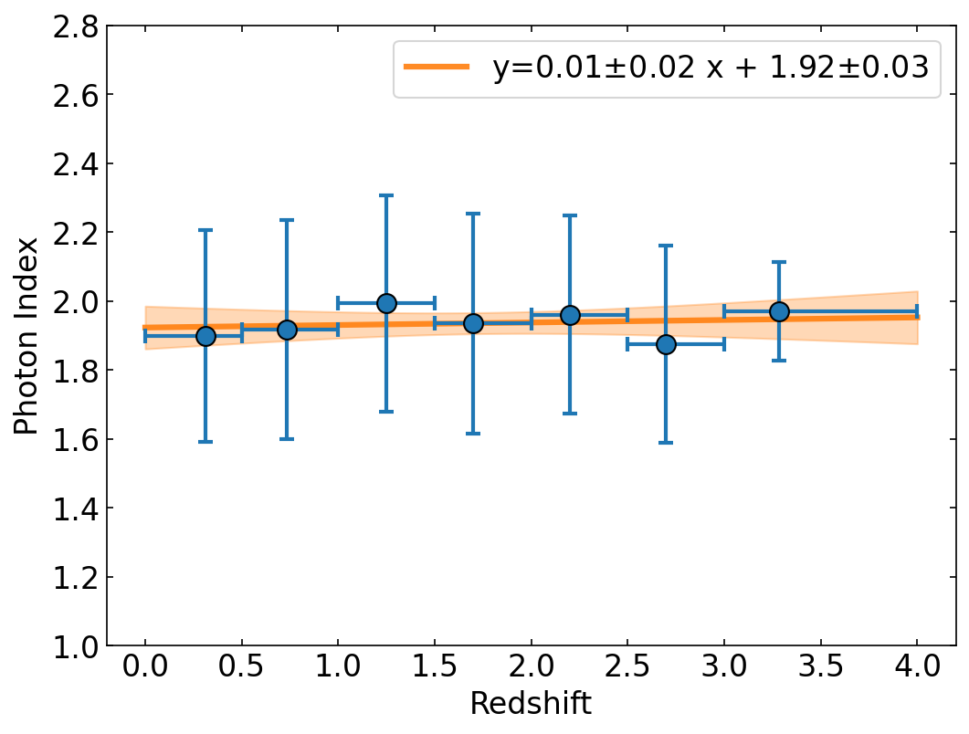
Figure 9: Photon index appears constant as a function of redshift. Values on the x-axis are centered at the redshift median value of each bin. Error bars on the y-axis represent one standard deviation in each bin, while on the x-axis represent the bin width. The best-fit line and its uncertainty at 2$\sigma$ are also shown (orange).

We were then able to estimate how many objects were lost in the analysis, and then derive the intrinsic number of sources by simply applying the correction to the observed data. Specifically, we corrected our sample on $L_{X}$, $N_{H}$, and $z$ bins according to the resolution of the simulation or, where not possible due to lack of sources, on larger bins. It is worth mentioning that we can correct only for the parameter space we detected. Which is to say, we can not correct for sources with, for example, $\log N_{\rm H}/\mathrm{cm}^{-2}>24$ and $\log L_{\rm X}/\mathrm{erg\,\,s}^{-1}>46$ since they were not available in our sample.

Figure 10: Loss surfaces for three luminosity values: $\log L_{\rm X}/\mathrm{erg\,\,s}^{-1}$ = 43.5 (yellow), 44.5 (green), and 45.5 (purple), as a function of redshift and absorption. See text for the fully explored parameter space. At each $N_{\rm H}$, and $z$, the corresponding $L_{\rm X}$ surface gives the fraction of sources lost in the S82X due to observational limits. Surfaces are smoothed for graphic purposes.

5.1.2 Sky coverage bias

The sky coverage of an X-ray survey is defined as the sky covered area as a function of the limiting flux. Thus, sources with different flux are detectable in different sky areas. This introduces a bias due to the AGN spectral shape, since it strongly depends on $N_{\rm H}$ and redshift. In particular, at a fixed redshift and luminosity, the sky coverage is biased against the detection of high-$N_{\rm H}$ AGN, which have lower fluxes than unobscured ones. This means that different AGN populations have different sky coverages as a function of $N_{\rm H}$ and $z$. We simulated 1000 sources for each set of parameters, as explained in Section 5.1.1, to quantify this effect. Then, we applied our count thresholds and derived the sensitivity curves. An example is shown in Figure 11.

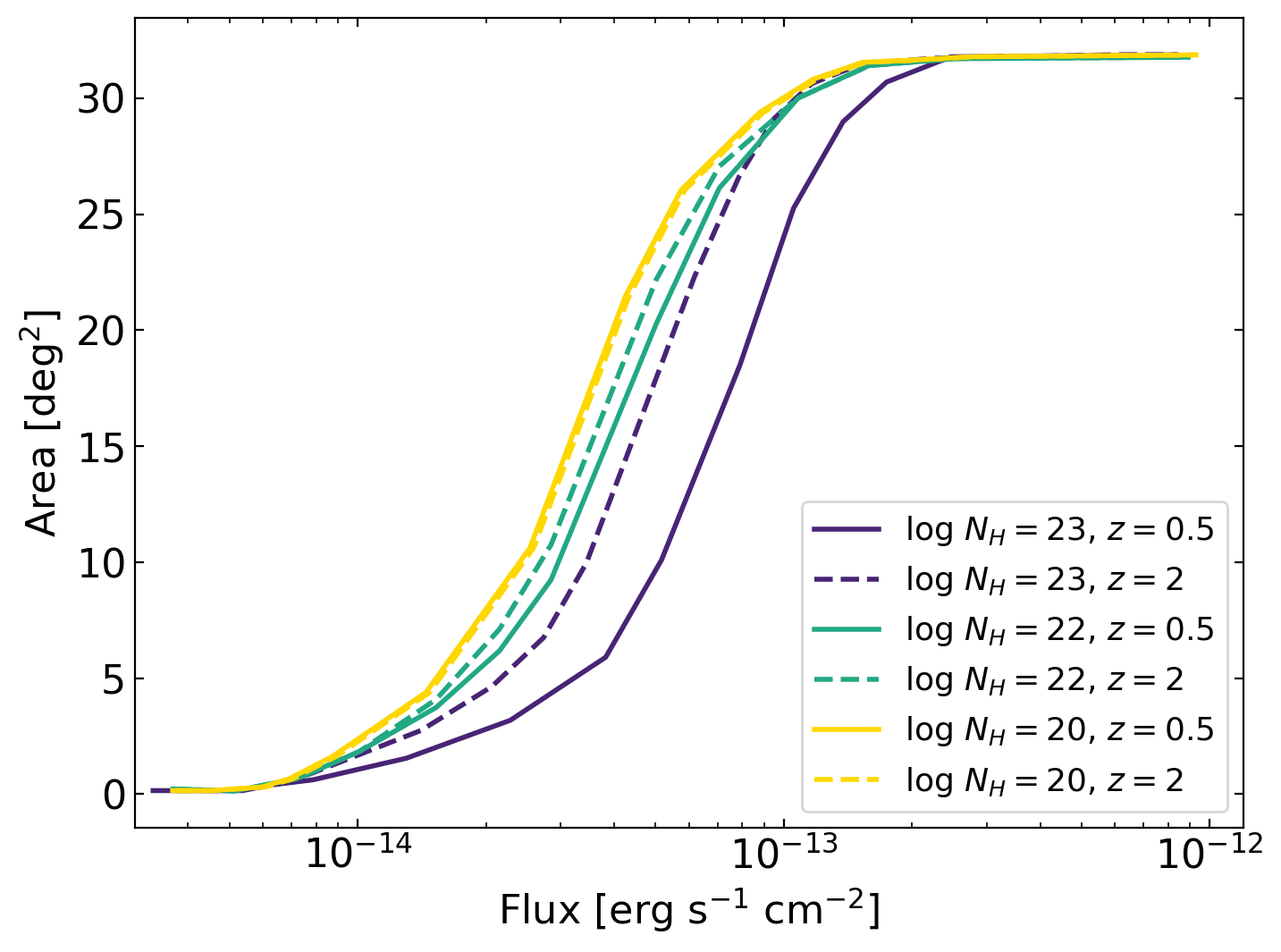
Figure 11: Sky coverage curves for $\log N_{\rm H}/\mathrm{cm}^{-2}=20$ (gold), 22 (green), and 23 (purple). Solid and dashed lines represent sensitivities at $z=0.5$ and 2, respectively. The sky coverage bias impacts negatively on high $N_{\rm H}$ sources, while the increasing redshift mitigates it because of a favorable K correction.

It is essential to notice that the sky coverage bias is independent of the Malmquist bias. Even if they both affect the detection of sources with high $N_{\rm H}$, the sky coverage bias compensates for the fact that different areas are sensitive to different observed fluxes, while the Malmquist bias depends on the intrinsic properties ($z$, $L_{\rm X}$, and $N_{\rm H}$) of the sources. We corrected for the sky coverage bias by weighting each source by the reciprocal of its sky coverage at the corresponding observed flux (e.g., Liu et al. 2017; Yuan et al. 2020). The weights were then included in the simulations performed in Section 5.1.1.

5.1.3 Eddington bias

Another effect to be considered is the Eddington bias (Eddington 1913). Since faint sources are more numerous than brighter ones, statistical fluctuations may boost their source counts, therefore leading to an overestimation of sources when count thresholds are used to select samples. We considered this effect by applying an additive correction similar to the one described in Liu et al. (2017): for each source in the main L16 catalog, we generated 1000 copies with counts drawn from a Poissonian distribution with mean number of counts corresponding to the value of the parent object. The resulting distribution for all replicated sources shows an excess of sources at low counts (Figure 12), reflecting the Eddington bias. The horizontal shift between the two distributions, shown in the lower panel, was assumed as pseudo-correction. In particular, we corrected for the Eddington bias by applying this pseudo-correction to our selection curves, obtaining effective counts thresholds that were used in the bias corrections described in Section 5.1.2 and 5.1.1. As shown by the bottom panel of Figure 12, the Eddington bias affects the sample selection by only $\sim$2 net counts or less, and is therefore almost negligible in our analysis.

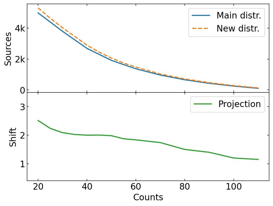
Figure 12: Upper panel: Smoothed, inverse cumulative counts distribution of the main catalog (solid blue) and of the simulated sample obtained by adding Poissonian fluctuations (dashed orange). Bottom panel: The projected horizontal shift between the two curves (solid green) was assumed to be a good approximation of the Eddington bias (see text). The curves are cut between 20 counts, below which no sources were selected, and 110 counts, after which the slope of the shift projection becomes steady.

5.1.4 Redshift completeness

To derive the properties of the intrinsic AGN populations, we must consider the redshift completeness of the sample, i.e., how many X-ray sources have a well constrained redshift estimate. S82X is almost 100% complete in redshifts; however, including only photometric redshifts with high probability (PDZ$\geq 70\%$), the redshift completeness drops to $\sim 75\%$. To verify that the remaining $\sim 25\%$ did not impact our results, we analyzed two test samples with redshift completeness of 90% and of 95%. Within the uncertainties, the obscured fractions and the derived XLF in those test samples were consistent with the 75% complete sample we analyze below (Section 5.2 and 5.3), with no systematic differences in the best-fit parameters. In addition, we performed a Kolmogorov-Smirnov (K-S) test between the 95% and 75% samples on the corresponding $N_{\rm H}$, $L_{\rm X}$, and $z$ distributions. The obtained $p$-values are 0.45, 0.27, and 0.33, respectively, indicating that the samples are not significantly different in those quantities. We conclude that sources missing due to redshift incompleteness do not introduce a bias in our results. In support of this conclusion, we note that low-quality photometric redshifts (PDZ$<70\%$) are not systematically inaccurate (e.g., all low or all high) if compared to their spectroscopic values.

5.2 Obscured fraction evolution

The obscured fraction is key to understand how obscured and unobscured AGN populations evolve through cosmic time. Moreover, complete knowledge of obscured accretion is essential to understanding AGN intrinsic luminosities and the overall accretion history of supermassive black holes, as well as how the two are linked (e.g., Hopkins et al. 2006). Once corrected for observational biases, the obscured AGN fraction was calculated as a function of redshift (Figure 13) and $L_{\rm X}$ (Figure 14). We defined the obscured fraction as the number of obscured, Compton-thin ($22\leq\log N_{\rm H}/\mathrm{cm}^{-2}<24$) AGN divided by the total number of AGN. Since we identified only two Compton-thick ($\log N_{\rm H}/\mathrm{cm}^{-2}\gtrsim 24$) sources, we focus here on the unobscured and Compton-thin populations. To avoid large uncertainties, we binned our data such that each bin contained at least 8 objects in both the numerator and denominator, with the exception of the red panel in Figure 14, where we used 6 objects as a minimum in order to have at least three points. Error bars in both the figures were computed with a bootstrapping procedure (e.g., Vito et al. 2018): the $N_{\rm H}$ distribution derived from the spectral analysis was used to generate a new random $N_{\rm H}$ distribution, with the same total number of sources and allowing for repetition. Then, a new obscured fraction was computed and the procedure was repeated 1000 times. At this point we had 1000 different values for each $N_{\rm H}$ bin, from which confidence intervals were computed.

First, we built the obscured, Compton-thin fraction ($F_{CN}$) as a function of redshift for three luminosity bins, from $\log L_{\rm X}/\mathrm{erg\,\,s}^{-1}=$43 to 46 erg (Figure 13). We assumed a broken power-law model in the following form:

$$F_{CN}(z)=\begin{cases}A(z/z_{*})^{-\alpha_{1}}&\text{if $z\leq z_{*}$}\\ A(z/z_{*})^{-\alpha_{2}}&\text{if $z>z_{*}$}\end{cases}$$ (7)

where $A$ is the normalization constant, and $z_{*}$ is the characteristic redshift between the two slopes $\alpha_{1}$ and $\alpha_{2}$. To fit the data points to the assumed model we used emcee (Foreman-Mackey et al. 2013), a solid Markov chain Monte Carlo (MCMC) implementation of the Goodman-Weare algorithm (Goodman & Weare 2010). The best-fit parameters are shown in Table 5.2 (top). We find that the obscured fraction increases with redshift at all luminosities. Formally, $z_{*}$ and $\alpha_{1}$ increase with luminosity, while no trend was found for $A$ and $\alpha_{2}$. Second, we built the obscured fraction as a function of $L_{\rm X}$, for four redshift bins from 0 to 4 (Figure 14). We assumed a simple line model, since we did not see any more complex trend in the data points, and applied the same fitting procedure described above. The best-fit results are shown in Table 5.2 (bottom). No trend was found in the best-fit parameters; however, the normalization in the selected luminosity range increases with the redshift. Our results are consistent with previous works (Treister & Urry 2006, Hasinger 2008, ; ; and A19) within the uncertainties (see also Section 5.6).

Overall, there is a strong positive redshift evolution, with the Compton-thin fraction increasing as a function of redshift at all luminosities. Moreover, the $z_{*}$ parameter increases with the luminosity bins, indicating a luminosity-dependent evolution. Indeed, we found an anti-correlation with the luminosity, at all redshifts. However, the uncertainties at high redshift and low luminosity, as well as those at low redshift and high luminosity, prevent us from further considerations on the luminosity-dependent evolution. Considering $\log L_{\rm X}/\mathrm{erg\,\,s}^{-1}>43$, and integrating over the redshift range 0-4, we obtained an obscured Compton-thin fraction of $57\pm 6\%$, while exploring the high $L_{\rm X}$ ($\log L_{\rm X}/\mathrm{erg\,\,s}^{-1}>45.5$) and high redshift ($z>3$) regime we obtained an obscured fraction of $64\pm 12\%$. This is consistent with what was found by e.g., B15 and A19.

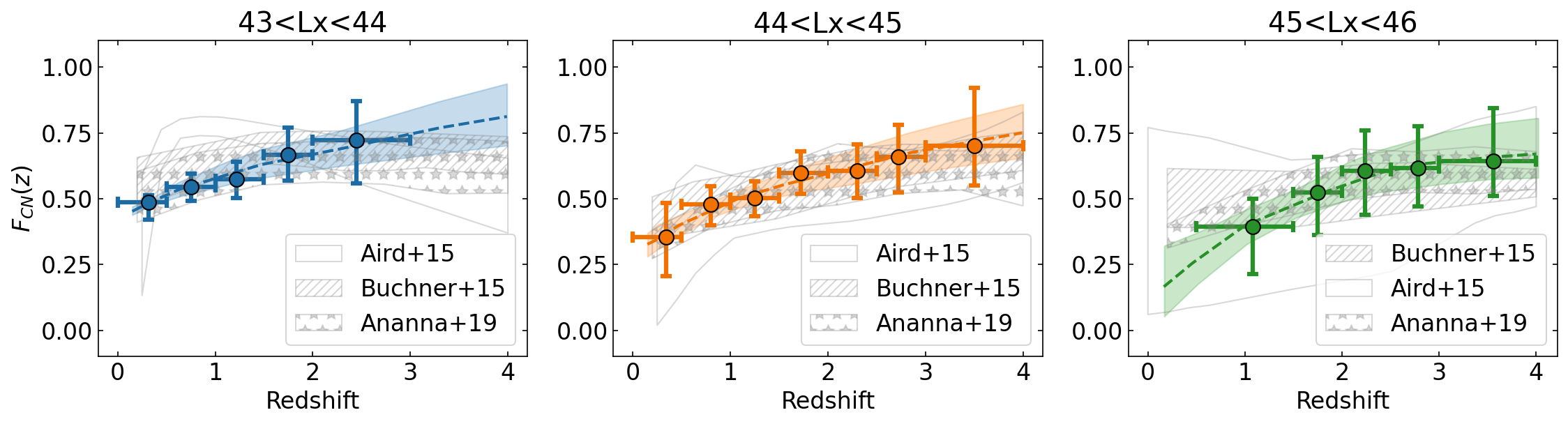
Figure 13: Obscured fraction evolution ($22\leq\log N_{\rm H}/\mathrm{cm}^{-2}<24$), corrected for observational biases, as a function of redshift for three $\log L_{\rm X}/\mathrm{erg\,\,s}^{-1}$ bins: 43 to 44 (left), 44 to 45 (middle), and 45 to 46 (right). The derived points overlaps the models from A19 (shaded stars), B15 (shaded slashed), and A15 (empty shaded). Error bars were obtained with a bootstrapping procedure (see text). Our models are shown with colored dashed lines in each panel, and the 1$\sigma$ confidence levels with colored shaded areas. In the x-axis, each point is centered at the median redshift value of the corresponding bin.

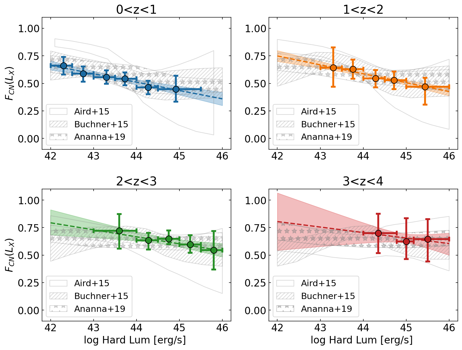
Figure 14: Same obscured fraction evolution represented in Figure 13, but as a function of intrinsic $L_{\rm X}$ in four redshift bins: 0 to 1 (upper left), 1 to 2 (upper right), 2 to 3 (lower left), and 3 to 4 (lower right). The derived points overlap the models from A19 (shaded stars), B15 (shaded dashed), and A15 (empty shaded). Error bars were obtained with a bootstrapping procedure (see text). On the x-axis, each point is centered at the median luminosity value of the corresponding bin.

Table 2: Fit Parameters for Evolution of Obscured Fraction

Obscured Fraction. vs. Redshift
Bin	$A$	$z_{*}$	$-\alpha_{1}$	$-\alpha_{2}$
$43<L_{\rm X}\leq 44$	0.58${}_{-0.05}^{+0.04}$	1.10${}_{-0.06}^{+0.05}$	0.14${}_{-0.04}^{+0.04}$	0.25${}_{-0.05}^{+0.05}$
$44<L_{\rm X}\leq 45$	0.52${}_{-0.04}^{+0.03}$	1.32${}_{-0.05}^{+0.04}$	0.25${}_{-0.04}^{+0.03}$	0.34${}_{-0.05}^{+0.04}$
$45<L_{\rm X}\leq 46$	0.60${}_{-0.07}^{+0.06}$	2.24${}_{-0.07}^{+0.06}$	0.55${}_{-0.06}^{+0.07}$	0.19${}_{-0.05}^{+0.06}$
Obscured Fraction vs. Luminosity
Bin	$m$		$q$
$0<z\leq 1$	$-0.076\pm 0.009$		$3.85\pm 0.04$
$1<z\leq 2$	$-0.081\pm 0.011$		$4.14\pm 0.07$
$2<z\leq 3$	$-0.064\pm 0.020$		$3.48\pm 0.09$
$3<z\leq 4$	$-0.05\pm 0.04$		$2.91\pm 0.19$

5.3 Luminosity function

The X-ray luminosity function is an important tracer of AGN evolution and is key to understand the accretion history of supermassive black holes. We built it using the corrected, (i.e., intrinsic) distributions of $N_{\rm H}$ and $L_{\rm X}$ derived from our analysis. One of the commonly used methods to build the XLF is the $1/V_{a}$ estimator (e.g., Miyaji et al. 2000), which is a generalization of the $1/V_{max}$ method (Schmidt 1968). The intuitive idea behind this method is to construct a binned differential luminosity function (LF) in redshift intervals. However, it may produce biases at low fluxes close to the data sensitivity and when the luminosity bins are large (see e.g., Page & Carrera 2000; Miyaji et al. 2001). Several methods were designed to address the limitations of the $1/V_{a}$ approach (e.g., Lynden-Bell 1971; Miyaji et al. 2001; Ananna et al. 2022); we used a method similar to Page & Carrera (2000), which works with Poissonian statistics, so there is no minimum number of objects required in each bin.

Our derived binned XLF ($\phi_{bin}$) is shown in Figure 15 (black points), for 7 redshift bins from $z=0$ to 4. The derived binned LF is consistent, within the uncertainties, with the XLFs from U14, A15, and A19. To fit the XLF, we applied the kernel density estimation (KDE) method described by Yuan et al. (2020, 2022). This nonparametric approach takes advantage of the mathematics beyond the KDE (Wasserman 2006), a well-established procedure to estimate continuous density functions (e.g., Chen 2017; Davies & Baddeley 2018). This method does not require any model assumptions, since it generates the XLF relying only on the available data. In particular, we apply the adaptive KDE version of the method, which automatically adapts the bandwidth of each individual kernel avoiding possible biases due to data inhomogeneity. The choice of the adaptive KDE is justified by applying a K–S test as described by Yuan et al. 2022 (Y22, hereafter). The analytical form of the adaptive KDE XLF, $\phi_{a}$ (for the full mathematical treatment, see Y22) is

$$\phi_{a}(z,L)=\frac{n(Z_{2}-Z_{1})\hat{f}_{a}(x,y|h_{10},h_{20},\beta)}{(z-Z_{1})(Z_{2}-z)\Omega dV/dz},$$ (8)

where [$Z_{1},Z_{2}$] is the dataset redshift range, $n$ is the number of objects in such range, $\Omega$ is the covered solid angle, $dV/dz$ is the the differential comoving volume per unit of solid angle, and $\hat{f}_{a}(x,y|h_{10},h_{20},\beta)$ is the density of $(x,y)$, which corresponds to the $(z,L)$ pair in the KDE parameter space. This function, $\hat{f}_{a}$, defined in equation A1 in Y22, depends on three parameters: the two bandwidths $h_{10}$ and $h_{20}$, which define the window width of the density estimation, and the sensitivity parameter, $\beta$, which allows for a flexible and adaptive kernel width. Y22 provide a Bayesian MCMC routine to determine the posterior distributions of the bandwidths and the $\beta$ parameter, and then the uncertainty estimation on the XLF.

The derived XLF is shown in Figure 15 (solid red lines and orange contours). In principle, the KDE method allows extrapolation of the XLF beyond the luminosity limits of the observations; however, the resulting high luminosity tail may overestimate the true XLF, especially when using the adaptive method (Yuan et al. 2020), so our XLFs are reported only for observed luminosities. As shown by the posterior error estimations in Figure 16, the derived best-fit parameters are well constrained, meaning a good kernel estimation (Y22).

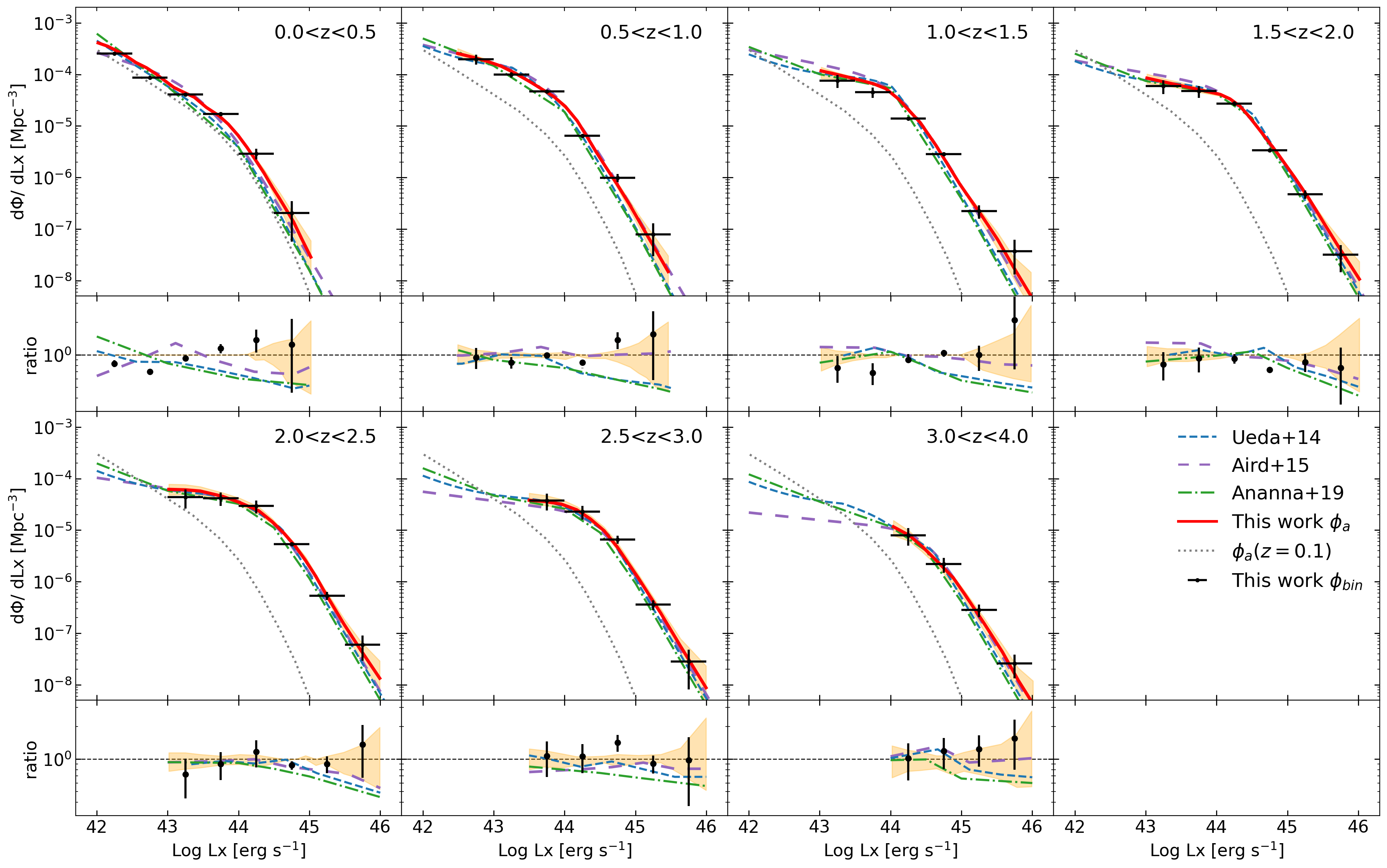
Figure 15: Derived XLFs for seven redshift bins. Black points represent the binned XLFs ($\phi_{bin}$, Page & Carrera 2000), while red solid lines show the KDE results ($\phi_{a}$, Y22) estimated at the redshift bin centers. For both methods, we calculate the XLF only where there are sufficient sources. Shaded orange regions represent the 3$\sigma$ uncertainties of the kernel density estimation. As a comparison, we show the XLFs derived by U14 (dashed blue), A19 (dash-dotted orange), and A15 (long dashed purple). All the XLFs were computed for $\log N_{\rm H}/\mathrm{cm}^{-2}<24$ AGN. The residuals, in the form of the ratio between each XLF and the KDE $\phi_{a}$, are shown at the bottom of each panel. The $z=0.1$ XLF (dotted black) derived with the KDE method is also plotted in each panel for reference.

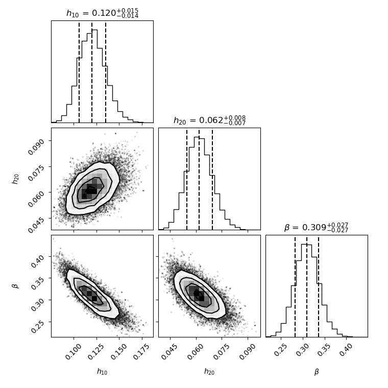
Figure 16: Posterior distributions of the bandwidths ($h_{10}$, $h_{20}$) and the $\beta$ parameter of the adaptive KDE XLF, obtained with the routine provided by Y22. Uncertainties correspond to the 16^th and 84^th percentiles, while the best fit value is the median. All the parameters are well constrained: $h_{10}=0.120_{-0.014}^{+0.015}$, $h_{20}=0.062_{-0.007}^{+0.008}$, and $\beta=0.309\pm 0.027$, meaning a good kernel density estimation of the XLF.

The XLF shows a strong luminosity evolution, since as the redshift increases the AGN density increases at high luminosity. We also see a density evolution, since the ratio between the XLF and the XLF at $z=0.1$ varies with $z$. In particular, the AGN density increases up to $z\sim 2$, then declines at $z\gtrsim 2.5$. These trends are in agreement with what was found previously by U14, A15, and A19. It is worth mentioning the differences among these works: U14 and A19 analyzed sources in the 0.5-195 keV range, while A15 analyzed the 0.5-7 keV band only (see also A19 for a detailed comparison), similar to the 0.5-10 keV range used in this work. Moreover, while they used different combinations of deep and wide surveys, we used the S82X data only. At the bottom of each panel in Figure 15, we plot the ratio between our XLF and the others (; ; ), showing they are in generally good agreement. Even though there is a slight increase of AGN densities at high luminosities, the uncertainties of both our XLF and the others (omitted in Figure 15 for clarity) become larger at these regimes, making them consistent within the errors and preventing us from further considerations. The nonparametric approach does not impose any particular shape on the XLF, but a break followed by significant steepening (a “knee” in the XLF), is required by the data. In practice, AGN at the break luminosity dominate the X-ray emission produced by the full population. This break luminosity evolves to higher luminosities with increasing redshift.

We also derived the XLF separately for obscured (CN) and unobscured AGN. The results are shown in Figure 17. Unobscured AGN slightly dominate at high luminosity ($\log L_{\rm X}/\mathrm{erg\,\,s}^{-1}\gtrsim$ 44-45) up to $z\sim 1.5$-2, with the obscured population dominating at lower luminosities. At higher redshifts ($z>2$), instead, the obscured population dominates at all luminosities. This is similar to what was found by A15. In general, both unobscured and obscured AGN experience strong luminosity evolution, as well as density evolution. Table 3 gives number densities for the total, unobscured, and obscured XLFs.

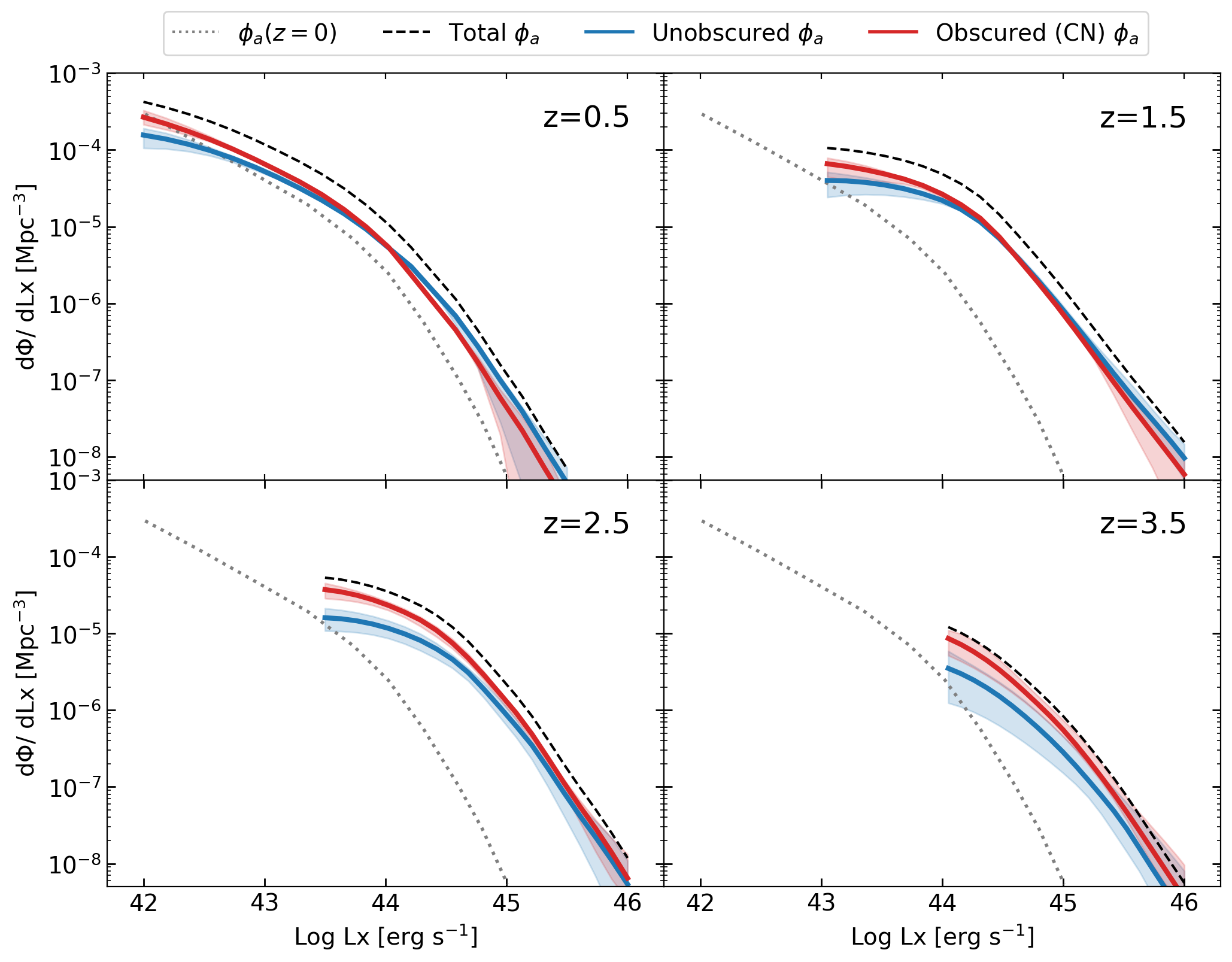
Figure 17: Total (dashed black), unobscured ($\log N_{\rm H}/\mathrm{cm}^{-2}<22$, solid blue) and obscured ($22\leq\log N_{\rm H}/\mathrm{cm}^{-2}<24$, solid red) XLFs derived with the KDE method (Yuan et al. 2022) for the corrected samples at $z=$ 0.5, 1.5, 2.5, and 3.5. Shaded regions represent the 3$\sigma$ uncertainties of the kernel density estimation. XLFs are cut off where we lack sources. The total XLF at $z=0.1$ (dotted black line) is also shown. The best-fit parameters are $h_{10}=0.192_{-0.028}^{+0.031}$, $h_{20}=0.047_{-0.012}^{+0.013}$, and $\beta=0.304_{-0.045}^{+0.044}$ for obscured AGN, and $h_{10}=0.170_{-0.025}^{+0.028}$, $h_{20}=0.071_{-0.009}^{+0.011}$, and $\beta=0.258_{-0.049}^{+0.049}$ for unobscured AGN.

In Figure 18 (top panel), we show the spatial AGN density as a function of redshift, for different luminosity bins. As the luminosity increases, the peak of the density moves towards higher redshifts. This pattern describes the so-called downsizing scenario (e.g., Cowie et al. 2003; Ueda et al. 2003), where the AGN density is driven by a combination of merger-driven mechanisms for high luminosity AGN, and secular processes dominated by minor mergers and disk instabilities for intermediate and low luminosity AGN (e.g., Treister et al. 2012; Miyaji et al. 2015). As we did for the XLF, we split the total AGN space density into unobscured and obscured populations (Figure 18, bottom panel). Except for the $\log L_{\rm X}/\mathrm{erg\,\,s}^{-1}$=42-43 bin, which is not covered adequately by our relatively shallow data, it is clear how the combination of the underlying populations models the total AGN density shape. In particular, the distributions of the two populations peak at different redshifts, with the obscured (unobscured) one at higher (lower) redshifts. This reflects the fact that obscured AGN become more dominant as the redshift increases.

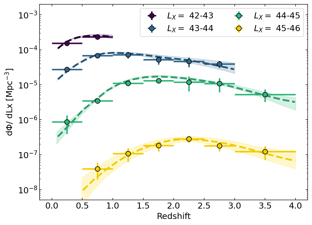
Figure 18: Top panel: Total AGN space density as a function of redshift and for $L_{\rm X}$ bins described in the legend. Dashed lines represent the derived XLF ($\phi_{a}$), while the points correspond to the binned XLF ($\phi_{bin}$), both integrated over corresponding the luminosity bin. Bottom panel: The black dashed lines are the same total space densities as in the top panel, each divided into unobscured (blue) and obscured (red) AGN populations. Shaded regions are the 3$\sigma$ uncertainties of the KDE estimation.

$\log L_{\rm X}$	$z$	$\phi_{a}$	$\phi_{unobs}$	$\phi_{obs}$
(erg s-1)	-	(Mpc-3)	(Mpc-3)	(Mpc-3)
42-43	0.1	$1.11_{-0.02}^{+0.03}\cdot 10^{-4}$	$4.29_{-1.00}^{+0.73}\cdot 10^{-5}$	$7.13_{-0.51}^{+0.88}\cdot 10^{-5}$
42-43	0.5	$2.39_{-0.04}^{+0.21}\cdot 10^{-4}$	$9.40_{-0.09}^{+0.16}\cdot 10^{-5}$	$1.51_{-0.01}^{+0.02}\cdot 10^{-4}$
42-43	1.0	$2.32_{-0.24}^{+0.34}\cdot 10^{-4}$	$9.18_{-1.59}^{+2.00}\cdot 10^{-5}$	$1.45_{-0.13}^{+0.18}\cdot 10^{-4}$
43-44	0.1	$1.49_{-0.05}^{+0.01}\cdot 10^{-5}$	$8.17_{-1.05}^{+1.42}\cdot 10^{-6}$	$6.64_{-0.65}^{+0.72}\cdot 10^{-6}$
43-44	0.5	$4.66_{-0.03}^{+0.41}\cdot 10^{-5}$	$2.13_{-0.02}^{+0.02}\cdot 10^{-5}$	$2.56_{-0.03}^{+0.04}\cdot 10^{-5}$
43-44	1.0	$8.16_{-0.31}^{+0.41}\cdot 10^{-5}$	$3.39_{-0.01}^{+0.05}\cdot 10^{-5}$	$4.77_{-0.07}^{+0.03}\cdot 10^{-5}$
43-44	1.5	$7.05_{-0.67}^{+0.88}\cdot 10^{-5}$	$2.71_{-0.45}^{+0.56}\cdot 10^{-5}$	$4.51_{-0.47}^{+0.33}\cdot 10^{-5}$
43-44	2.0	$5.67_{-0.80}^{+0.82}\cdot 10^{-5}$	$1.90_{-0.42}^{+0.33}\cdot 10^{-5}$	$4.09_{-0.51}^{+0.68}\cdot 10^{-5}$
43-44	2.5	$4.15_{-0.71}^{+1.15}\cdot 10^{-5}$	$1.27_{-0.27}^{+0.38}\cdot 10^{-5}$	$3.17_{-0.44}^{+0.49}\cdot 10^{-5}$
43-44	3.0	$2.92_{-0.71}^{+1.30}\cdot 10^{-5}$	$9.26_{-2.05}^{+2.70}\cdot 10^{-6}$	$2.15_{-0.43}^{+0.44}\cdot 10^{-5}$
44-45	0.1	$3.37_{-1.04}^{+1.37}\cdot 10^{-7}$	$2.41_{-0.47}^{+0.76}\cdot 10^{-7}$	$1.04_{-0.33}^{+0.61}\cdot 10^{-7}$
44-45	0.5	$1.92_{-0.27}^{+0.19}\cdot 10^{-6}$	$1.07_{-0.10}^{+0.06}\cdot 10^{-6}$	$8.49_{-0.39}^{+0.45}\cdot 10^{-7}$
44-45	1.0	$8.47_{-0.23}^{+0.74}\cdot 10^{-6}$	$4.18_{-0.38}^{+0.32}\cdot 10^{-6}$	$4.31_{-0.41}^{+0.32}\cdot 10^{-6}$
44-45	1.5	$1.54_{-0.34}^{+0.17}\cdot 10^{-5}$	$7.07_{-0.62}^{+0.65}\cdot 10^{-6}$	$8.54_{-0.80}^{+0.29}\cdot 10^{-6}$
44-45	2.0	$1.62_{-0.06}^{+0.13}\cdot 10^{-5}$	$6.89_{-0.25}^{+0.23}\cdot 10^{-6}$	$9.57_{-0.41}^{+0.29}\cdot 10^{-6}$
44-45	2.5	$1.28_{-0.11}^{+0.09}\cdot 10^{-5}$	$4.70_{-0.49}^{+0.58}\cdot 10^{-6}$	$8.50_{-0.63}^{+0.41}\cdot 10^{-6}$
44-45	3.0	$8.55_{-0.60}^{+1.42}\cdot 10^{-6}$	$2.91_{-0.51}^{+0.85}\cdot 10^{-6}$	$5.93_{-1.10}^{+0.59}\cdot 10^{-6}$
44-45	3.5	$5.19_{-1.03}^{+1.06}\cdot 10^{-6}$	$1.74_{-0.49}^{+0.56}\cdot 10^{-6}$	$3.63_{-0.81}^{+0.58}\cdot 10^{-6}$
44-45	4.0	$3.02_{-1.24e}^{+1.13}\cdot 10^{-6}$	$8.98_{-3.35}^{+4.74}\cdot 10^{-7}$	$2.24_{-0.72}^{+0.89}\cdot 10^{-6}$
45-46	0.5	$9.87_{-6.20}^{+12.3}\cdot 10^{-9}$	$6.43_{-4.62}^{+8.55}\cdot 10^{-9}$	$3.53_{-3.42}^{+5.03}\cdot 10^{-9}$
45-46	1.0	$5.46_{-2.15}^{+3.02}\cdot 10^{-8}$	$3.33_{-1.21}^{+1.56}\cdot 10^{-8}$	$2.16_{-0.72}^{+1.12}\cdot 10^{-8}$
45-46	1.5	$1.65_{-0.51}^{+0.39}\cdot 10^{-7}$	$8.44_{-1.22}^{+3.43}\cdot 10^{-8}$	$8.04_{-1.69}^{+2.49}\cdot 10^{-8}$
45-46	2.0	$2.70_{-0.54}^{+0.44}\cdot 10^{-7}$	$1.28_{-0.33}^{+0.39}\cdot 10^{-7}$	$1.44_{-0.29}^{+0.46}\cdot 10^{-7}$
45-46	2.5	$2.63_{-0.40}^{+0.38}\cdot 10^{-7}$	$1.14_{-0.24}^{+0.37}\cdot 10^{-7}$	$1.54_{-0.19}^{+0.65}\cdot 10^{-7}$
45-46	3.0	$1.96_{-0.64}^{+0.33}\cdot 10^{-7}$	$7.64_{-2.04}^{+4.56}\cdot 10^{-8}$	$1.26_{-0.16}^{+0.41}\cdot 10^{-7}$
45-46	3.5	$1.24_{-0.45}^{+0.40}\cdot 10^{-7}$	$3.46_{-1.46}^{+3.87}\cdot 10^{-8}$	$6.18_{-1.50}^{+4.87}\cdot 10^{-8}$
45-46	4.0	$7.14_{-3.20}^{+5.96}\cdot 10^{-8}$	$1.96_{-1.13}^{+3.01}\cdot 10^{-8}$	$3.55_{-1.65}^{+3.66}\cdot 10^{-8}$

Table 3: Numerical values for the derived XLFs: total ($\phi_{a}$), unobscured ($\log N_{\rm H}/\mathrm{cm}^{-2}<22$, $\phi_{unobs}$), and obscured ($22\leq\log N_{\rm H}/\mathrm{cm}^{-2}<24$, $\phi_{obs}$), for different luminosity and redshift bins. Uncertainties are reported at 3$\sigma$ confidence level on the kernel density estimation.

5.4 Black hole accretion density

AGN evolution can be further analyzed by computing the black hole accretion density (BHAD, or $\Psi_{\rm BHAD}$), which encapsulates the SMBH growth history (e.g., Soltan 1982). The BHAD is defined as

$$\Psi_{\rm BHAD}(z)=\int\frac{(1-\epsilon)}{\epsilon c^{2}}L_{\rm bol}\phi(L_{\rm bol},z)d\log L_{\rm bol}\,\,\mathrm{[cgs]},$$ (9)

where $\epsilon$ is the radiative efficiency (here assumed to be $\epsilon=0.1$; e.g., Hopkins et al. 2007; Vito et al. 2018), $L_{\rm bol}$ is the bolometric luminosity, and $\phi(L_{\rm bol},z)$ is the bolometric luminosity function at a given redshift. We derived $L_{\rm bol}$ and $\phi(L_{\rm bol},z)$ from their X-ray analogues by applying the bolometric correction found by Duras et al. (2020). Due to the large scatter in these values (e.g., Lusso et al. 2012; Duras et al. 2020), we also applied the bolometric correction derived by Hopkins et al. (2007), which is higher in the range $\log L_{\rm X}/\mathrm{erg\,\,s}^{-1}\sim$42-45, but lower at higher luminosities. The differences in these bolometric corrections dominate the uncertainties in the BHAD. Equation (9) is ideally integrated over all luminosities (e.g., Delvecchio et al. 2014). Practically, we selected the $\log L_{\rm bol}$ range corresponding to $\log L_{\rm X}/\mathrm{erg\,\,s}^{-1}$=42-47. Since our derived XLF do not cover entirely this range, we extrapolated our results as follows. Motivated by the fact that the main contribution to the AGN accretion rate is produced by the break luminosity of the XLF, which we constrained at all redshifts, and that XLF models have typically double power-law shapes (e.g., Vito et al. 2014, A15), we extended our XLF by maintaining constant the average slope before and after the break luminosity. Since at $z\gtrsim 3$ our XLF is poorly constrained at low luminosities, we assumed the A15 slope, whose XLF best overlaps with ours (see Figure 15).

Our derived BHAD is shown in Figure 19, along with several other estimates for comparison. First, we show the BHAD derived from the A19 XLF because it was based on the most comprehensive data available, including hard X-ray surveys from NuSTAR and Swift-BAT, which are sensitive up to $\sim 195$ keV and thus identify highly obscured sources that otherwise could be missed at lower energies (e.g., Gilli et al. 2007; Treister et al. 2009; Ballantyne et al. 2011). Moreover, the A19 model simultaneously reproduces number counts from the largest surveys over different areas and depths, as well as constraints from the cosmic X-ray background, and is therefore the most up-to-date population synthesis model for AGN. In any case, due to the similarities between our XLF and the other X-ray XLFs, their BHADs are similar to ours. Considering Compton-thin AGN only (hatched green), the BHAD derived from A19 agrees well with our curve (solid blue). The complete A19 BHAD (solid green) is a factor $\sim$2-3 higher, as expected because of the substantial number of Compton-thick AGN, which are not well sampled in our survey nor other samples (e.g., U14, A15).

The yellow region in Figure 19 was derived by Delvecchio et al. (2014) from Herschel infrared observations of AGN, using decomposition of UV-optical-infrared spectral energy distributions (SEDs) to isolate the emission from black hole accretion. However, this procedure may miss some AGN when the SED is dominated by stellar emission (e.g., Delvecchio et al. 2017), especially if the AGN radiation is buried behind obscuring material (e.g., Del Moro et al. 2013; Hatcher et al. 2021). Hence, it is not surprising that the Delvecchio et al. (2014) infrared curve lies near or below our curve; indeed, this comparison suggests that the SED-decomposition approach could miss the majority of Compton-thick AGN, or at least a significant fraction of them.

Theoretical simulations of black hole growth from Sijacki et al. (2015) and Volonteri et al. (2016) are also shown in Figure 19 (purple curves). These models are similar to the A19 curve, although slightly different in shape, and they lie well above our curve, particularly for $z\gtrsim 2$. The discrepancy between X-rays and theoretical simulations is known in the literature (e.g., Vito et al. 2018; Barchiesi et al. 2021), and it is generally explained with the challenges in efficiently detecting heavily obscured, Compton-thick sources in X-ray surveys (e.g., Hickox & Alexander 2018). These tensions suggest that Compton-thick AGN may have a substantial role in the supermassive black holes accretion history, especially at high redshift, even though their contribution is still not well understood.

We also compare our results with the star formation rate densities (SFRD) found by Madau & Dickinson (2014) and Bouwens et al. (2015) (in grey, scaled down by a factor $2\times 10^{4}$ to avoid confusion with the other curves). As for the BHAD, there is a peak around redshift $z\sim 2$. The similar evolution of the BHAD and SFRD is considered evidence in favor of the SMBH host galaxy co-evolution scenario (e.g., see Vito et al. 2018 or Hickox & Alexander 2018 for a review). In detail, however, these quantities seem to have a different evolution, especially at high redshifts. In particular, the slope of the BHAD at $z>2$ is steeper than that of the SFRD, implying that black holes grow faster, on shorter time scales, compared to their host galaxies (e.g., A15). However, the large uncertainties in deriving the BHAD and the SFRD from different observations, simulations, and methods, leave the discussion open.

Figure 19: Evolution of the black hole accretion density (BHAD) derived in this work (blue curves), compared with A19 (green curves, with and without Compton-thick AGN), and the theoretical works of Sijacki et al. (2015) (shaded purple) and Volonteri et al. (2016) (purple line). The continuous and dashed lines correspond to the BHADs derived with the bolometric corrections of Duras et al. (2020) and (Hopkins et al., 2007), respectively. The Delvecchio et al. (2014) BHAD, obtained from infrared data, is also shown (shaded yellow). For comparison, we added the Madau & Dickinson (2014) and Bouwens et al. (2015) star formation rate densities (scaled by a factor $2\times 10^{4}$ for clarity, grey dotted line and grey dashed area, respectively).

5.5 On the evolutionary picture

Our analysis shows how the total AGN space density evolves over cosmic time, and how its shape depends on the interplay between unobscured and obscured AGN. We now discuss models that might explain the observed trends with luminosity, obscuration, and redshift.

One of the most invoked models to explain the decreasing obscured fraction with increasing X-ray luminosity is the receding torus model (e.g., Lawrence 1991; Simpson 2005). In this model, a decrease in the covering factor of the dusty torus (e.g., Buchner et al. 2015; Matt & Iwasawa 2019) is caused by increasing radiation pressure, photoionization of gas clouds, dust sublimation, or some combination thereof (e.g., Hönig & Beckert 2007; Akylas & Georgantopoulos 2008; Mateos et al. 2017). The receding torus model therefore links the distribution of line-of-sight column densities and intrinsic luminosity. However, it is unclear how to connect this model to the redshift evolution, since it predicts less obscuration at higher redshifts, where AGN are on average more luminous, whereas the opposite trend is observed.

Another common picture is that luminous AGN are triggered by mergers (e.g., Sanders et al. 1988; Treister et al. 2012), which supply gas to the black hole (Hopkins et al. 2006; Somerville et al. 2008) and, at least initially, produce high levels of obscuration (e.g., Sanders et al. 1988; Blecha et al. 2018). During this stage, the SMBHs grow close to the Eddington limit, generating a combination of radiation and kinetic pressure capable of blowing out gas and dust around the central engine, leading to a largely unobscured phase (Sanders et al. 1988, Treister et al. 2010) during which the AGN shines until the accretion processes consumes the gas reservoir (e.g., Hopkins et al. 2008). It is therefore likely that high-luminosity AGN generate efficient feedback mechanisms capable of depleting and consuming the gas supply (e.g., B15), linking the X-ray luminosity to the accretion processes (e.g., Hopkins et al. 2007, U14). In this scenario, one expects the fraction of unobscured sources to increase with luminosity, in any redshift bin, as observed (Fig. 17). At the same time, for fixed luminosity, the fraction of unobscured sources should decrease with increasing redshift because mergers, and obscuration in general (e.g., Carilli & Walter 2013), become more common at high redshift (e.g., Ricci et al. 2017b). Both trends are observed in our results (bottom panel of Fig. 18).

Hopkins et al. (2005) proposed an interpretation of the AGN luminosity function in which the bright end corresponds to AGN at the maximum of their accretion history, while the faint end traces AGN during small accretion events either at the beginning or the end of their activity peak. The bulk of AGN accretion is then produced by the “knee” of the LF, where the density of AGN at their activity peak is maximized. Both the XLF density evolution and the BHAD derived in this work show a peak at $z\sim 2$. At these redshifts, obscured AGN dominate for $\log L_{\rm X}/\mathrm{erg\,\,s}^{-1}>43$ (Fig. 17), meaning the majority of black hole accretion occurs in an obscured stage.

5.6 Comparison to Other Works

In this work, we analyzed the X-ray spectra of AGN from the S82X sample, then derived the intrinsic distributions and luminosity functions of X-ray-selected AGN by correcting for observational biases (Section 5.1). In particular, we used simulations to correct for Malmquist bias (loss of faint sources at the flux limit), sensitivity bias (from the range of spectral shapes), and Eddington bias (statistical fluctuations near the flux limit). We did not assume any functional form for the XLF, $N_{\rm H}$ distributions, or X-ray spectra, allowing these to be dictated by the data (and bias corrections). Because we used only observations from the S82X survey, we avoided the challenge of correcting for different survey sensitivities.

We were able to measure the evolving XLF and place strong constraints on the obscured fraction up to $z=4$ because of the many S82X AGN with $z>3$ and $\log L_{\rm X}/\mathrm{erg\,\,s}^{-1}>45.5$. Previous results based on smaller, deeper surveys, which lack sources in this redshift and luminosity regime, are usually extrapolated or less well constrained. Our results agree well with those of U14, B15, and A19; A15 predicts more obscured AGN at $z\lesssim 1$, and with different trends at $\log L_{\rm X}/\mathrm{erg\,\,s}^{-1}$ 43-44, but is consistent at all other redshifts and luminosities. It is worth noticing that Georgakakis et al. 2017 derived a slightly lower fraction of obscured AGN at $z\sim 1$ and $\log L_{\rm X}/\mathrm{erg\,\,s}^{-1}$ 44-45 in XMM-XLL, but consistent with ours within the errors. Moreover, our derived obscured AGN fractions are consistent, within the uncertainties, also with Treister & Urry 2006 and Hasinger 2008, which derived the obscured fraction of AGN relying on optical classification and using a combination of optical spectra and X-ray photometry, respectively.

The effects of our non-parametric approach can be seen in a less evident “knee” in the XLF and by a slope that can change with redshift and luminosity, instead of having a fixed number of slopes dictated by the model (Figure 15). We also have sufficient obscured AGN to determine the XLF independently for Compton-thin and unobscured AGN separately (Fig. 17). Other XLFs at high redshift ($z>3$) and high luminosity ($\log L_{\rm X}/\mathrm{erg\,\,s}^{-1}>45.5$) have usually been obtained using mainly unobscured sources, using assumptions or extrapolations to derive information on the underlying obscured population (e.g., Hickox & Alexander 2018). Commonly adopted solutions are: i) extrapolating local obscured AGN distributions up to high redshift (e.g., U14), ii) using only a few objects to constrain the obscured fractions (e.g., B15), or iii) including additional information such as constraints from the X-ray background (e.g., Gilli et al. 2007, A19). However, these approaches generally fail, if taken individually, to satisfy all current available data (see comparisons by A19).

5.7 Compton-thick AGN

We were able to place strong constraints on unobscured and Compton-thin AGN, but the role of highly obscured, Compton-thick AGN is difficult to analyze with the S82X sample alone (see also Section 5.4). We found just two Compton-thick objects plus three other candidates (which have $N_{\rm H}$ upper limits above $10^{24}$ cm^-2). Figure 20 compares these numbers with the number of expected Compton-thick AGN from the Gilli et al. (2007) and A19 models, taking into account the S82X limiting flux and the cuts we applied on the number of counts, but not the selection in photometric redshifts. In particular, the latter may be crucial in recovering the full number of these highly obscured sources, since they are usually faint and difficult to detect in optical/infrared bands. Thus, these predictions have to be considered as upper limits.

The total number of predicted Compton-thick AGN in the redshift range 0-4 is $\sim$4.5 and $\sim$7.6 for the two models, respectively. Given the limited statistics, these numbers are consistent with what we found, although three of five sources have only $N_{\rm H}$ upper limits, and thus their interpretation as Compton-thick sources is uncertain. This result suggests that to investigate the intrinsically luminous, Compton-thick population we need much larger numbers of AGN, either from wider areas or deeper observations. This is especially true at $z\gtrsim 2$, where the number of detected highly obscured AGN should drop dramatically due to their faintness (e.g., Treister et al. 2004).

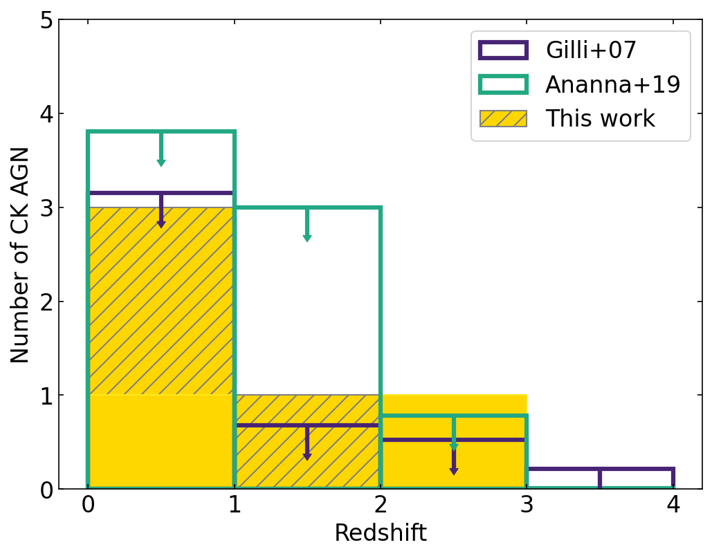
Figure 20: The number of Compton-thick AGN ($\log N_{\rm H}/\mathrm{cm}^{-2}=$ 24-26) identified in this work (gold) is in good agreement with the predicted number from Gilli et al. 2007 (purple line) and Ananna et al. 2019 (green line), albeit with limited statistics. Hatched regions correspond to $N_{\rm H}$ upper limits above $\log N_{\rm H}/\mathrm{cm}^{-2}=$ 24. Model predictions are upper limits because of our quality cut on the photometric redshifts.

6 Future prospects

Population studies with high luminosity and high redshift AGN strongly depend on the number of objects available in such extreme regimes. In this work, we used the available S82X data from L16 and LaMassa et al. 2019a, which allowed us to investigate AGN up to $z=4$ and $\log L_{\rm X}/\mathrm{erg\,\,s}^{-1}=46$ for both unobscured and obscured (Compton-thin) AGN populations. To overcome these limits, larger samples are needed. Since L16, there are new XMM-Newton and Chandra archival observations in the Stripe 82 field, such that the total non-overlapping area reaches $\sim 50$ deg². Taking into account also overlapping observations, we estimate to almost double the current number of objects and to increase the overall depth by a factor of $\sim 2$. This will be a significant improvement over our current results, especially for the Compton-thick AGN population. We note that the study of obscured AGN populations in particular will benefit from the Herschel and Spitzer infrared data available in the S82X, which helps determine photometric redshifts (e.g., Salvato et al. 2009; Ananna et al. 2017; Peca et al. 2021) and improves analysis of spectral energy distributions (Auge et al., in prep.). Moreover, we are continuing spectroscopic follow-up of S82X sources (LaMassa et al. 2019a), meaning that the number of spectroscopic redshifts will grow in the next years, adding more sources to the X-ray spectral analysis sample.

Another approach is to include other X-ray surveys in the analysis (e.g., ; ; ; ). Deep X-ray surveys can reveal heavily obscured sources, but typically cover very small volumes, and thus are not sensitive to rare objects at high luminosity (e.g., Marchesi et al. 2016; Liu et al. 2017). Even the XMM-XXL field (XXL North, $\sim 25$ deg²) has only 5 objects at $\log L_{\rm X}/\mathrm{erg\,\,s}^{-1}>45.5$, all of them classified as broad-line AGN from optical spectra (Liu et al. 2016), and S82X AGN ($\sim 31$ deg²) do not exceed $\log L_{\rm X}/\mathrm{erg\,\,s}^{-1}=46$. Much larger surveys, such as eFEDS (Brunner et al. 2022) and the forthcoming all-sky eROSITA survey (Merloni et al. 2012), will be needed to detect rare and intrinsically luminous objects. Even then, eROSITA has less effective area than XMM-Newton above 3 keV, and higher background than Chandra, so it is relatively less sensitive to obscured AGN. For example, only 245 sources—$\sim 1$% of the current eFEDS catalog—are detected in the hard band (2.3-5 keV). Of course, since the eROSITA final all-sky catalog (eRASS:8, Predehl et al. 2021) will have millions of extragalactic sources, even the obscured ones will be available in large numbers, enough to allow population studies. However, the corrections for obscured AGN missed by the soft-band selection will be large.

Moreover, data above 10 keV are fundamental to detecting heavily obscured sources and Compton-thick AGN (e.g., Ricci et al. 2017a; A19; Marchesi et al. 2019; Koss et al. 2022). The combination of these very hard-band X-ray observations and simulations (e.g., Baloković et al. 2021) to correct for observational biases is crucial to constrain the fraction of Compton-thick AGN and, therefore, to shed light on the black hole accretion in the young Universe and on the onset of the black hole-galaxy co-evolution.

Future planned X-ray telescopes will certainly improve our current knowledge of AGN populations. For example, the planned AXIS mission (Mushotzky et al. 2019) is designed to have an effective area of roughly 7 (2) and 25 (5) times those of the current XMM-Newton and Chandra capabilities at 1 (6) keV, respectively, with sub-arcsecond angular resolution over a $24\arcmin\times 24\arcmin$ field of view. This will be an improvement of a factor of $\sim$100 with respect to Chandra, whose PSF degrades rapidly outside $2\arcmin$. Marchesi et al. (2020) predicted that AXIS would detect more than 200,000 AGN in the 0.5-7 keV band, including $>7000$ at $z>3$ and tens at $z>6$, from a combination of deep, intermediate, and wide surveys. This is just one example of possible next-generation telescopes—like Athena (Barret et al., 2020) and Lynx (Gaskin et al., 2019)— which will be essential to better constraining the obscured fraction and XLF at the highest redshifts and luminosities, and to unveiling a new window for AGN population studies in the Universe up to $z\sim 8$ (Marchesi et al. 2020).

7 Summary

We exploited the full extent of X-ray and multiband data in the S82X field by analyzing the X-ray spectra of the 2937 sources with a solid redshift estimate (L16, LaMassa et al. 2019a). Using simulations, we established thresholds for the minimum number of detected counts needed to get a reliable fit. We considered simple power-law models as well as more complex shapes, including soft-excess and reflection components. The best fits were then identified using the AIC criterion.

We derived the evolving AGN X-ray luminosity function, correcting for observational biases through extensive simulations, and without assuming any particular functional form. In addition to the total XLF, we derived separate XLFs for obscured and unobscured AGN populations, and we computed the obscured fraction of AGN as a function of both redshift and luminosity. S82X AGN with high luminosities ($L_{\rm X}>45.5$ erg s^-1) and redshifts ($z>3$) add new statistical weight not available from smaller volume surveys.

Our XLF shows a “knee” imposed by the data, which represents where AGN dominate the luminosity at a particular redshift. The shape of the total XLF exhibits both luminosity and density evolution: AGN are more luminous at higher redshift and, for fixed luminosity, have higher densities at lower redshift. The unobscured and obscured XLFs, whose combination constitutes the total XLF in changing contributions, reveal that obscured AGN dominate at all luminosities at $z>2$. The fraction of AGN that are obscured increases with redshift, and decreases with increasing luminosity.

We used the XLF to compute the black hole accretion density as a function of redshift. Although our BHAD has a similar shape compared to other works based on Compton-thin AGN, it lies below theoretical predictions. Including Compton-thick AGN roughly doubles the emission and largely resolves the disagreement with theory, even if the slightly different shapes of the curves remain to be explained. This result suggests that Compton-thick AGN have an essential role in the growth of supermassive black holes, and that their contribution exceeds previous estimates (e.g., ; ). The BHAD for X-ray-selected AGN lies above estimates from far-infrared-selected AGN, implying that, at least with present flux limits, infrared surveys may miss Compton-thick AGN.

The patterns found for the XLFs, obscured fractions, and BHAD confirm the cosmic downsizing of black hole growth. The similar evolution of the black hole and star formation densities supports the idea of co-evolution between SMBH and host-galaxy, but suggesting different time scales during their evolution.

Current and upcoming X-ray surveys with larger volumes will increase the statistics of AGN at high luminosity, high obscuration, and high redshift beyond the work presented here. This includes both future surveys with eROSITA and proposed X-ray observatories, and newer archival X-ray observations in S82X, which have the advantage of invaluable ancillary multiwavelength data, especially in the infrared.

Appendix A Background modeling

In this section, we describe the models adopted to fit the backgrounds in the XMM-Newton and Chandra data. The observed X-ray background is composed of two main components: cosmic and instrumental (blue and orange curves in Fig. 21, respectively). The cosmic background is produced by the sum of Galactic and extragalactic components:

• Two thermal components (XSPEC model apec; e.g., Lanzuisi et al. 2015) representing a local hot bubble ($kT\sim 0.04$ keV) and interstellar gas in the Galactic disk ($kT\sim 0.12$ keV) (Kuntz & Snowden, 2000);

• The extragalactic X-ray background produced by unresolved emission from discrete sources (e.g., Comastri et al. 1995), which can be modeled with a $\Gamma\sim 1.4$ power-law, modified by Galactic absorption (e.g., De Luca & Molendi 2004).

The instrumental background is the sum of three main components:

• Several emission lines produced by the telescope instrumentation, which we modeled with a combination of Gaussian lines (see Table 4);

• Residuals from the filtering of quiescent soft protons (QSP, e.g., Baldi et al. 2012);

• The cosmic ray-induced continuum (NXB, Leccardi & Molendi 2008).

The QSP and NXB were modeled with two broken power-laws for XMM-Newton (e.g., Leccardi & Molendi 2008), and with a single broken power-law plus a broad Gaussian line above $\sim$ 5 keV for Chandra. For Chandra only, we also added a broad Gaussian line between 1 and 3 keV (Fiore et al. 2012), which may be a mother-daughter artifact produced during the Charge Transfer Inefficiency (CTI) correction (Bartalucci et al. 2014). Table 4 summarizes these components.

It is worth noticing that for both XMM-Newton and Chandra, we repeated the above modeling using backgrounds extracted from two different epochs: from the oldest observations to 2008, and from 2010 to the most recent, to check for possible differences due to the effective area degradation of the telescopes. Once the background best-fit was obtained, we fitted a sub-sample of 1000 random sources using the derived backgrounds. Since we found that the derived fluxes, $N_{\rm H}$, and luminosities were consistent within each other, we modeled the background using the set of observations described in Section 3.2 .

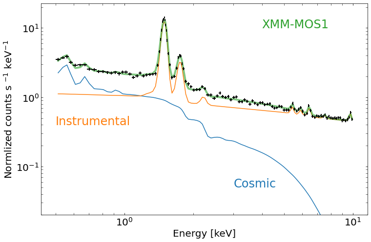
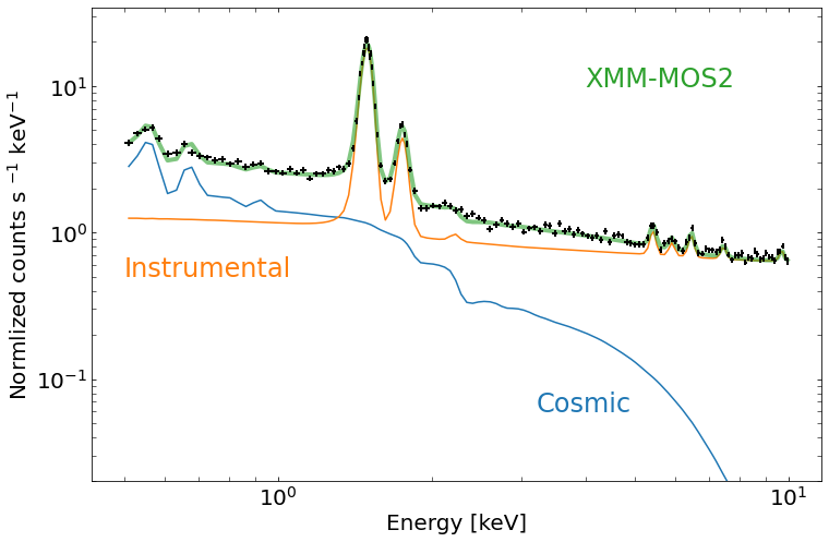
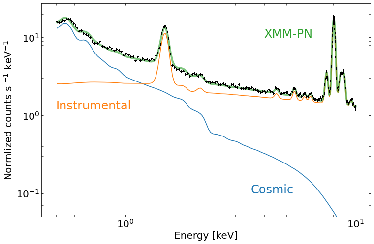
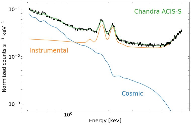
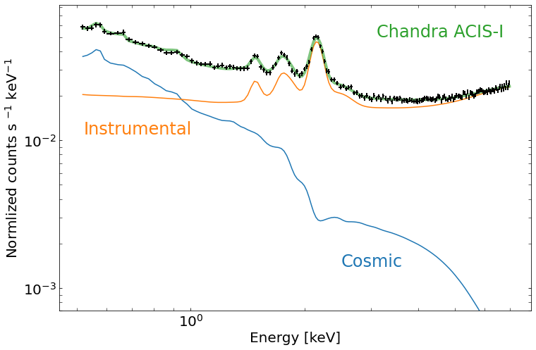
Figure 21: Background spectra used in the background modeling procedure. From the top-left panel: XMM-Newton MOS1, MOS2, PN, Chandra ACIS-S, and ACIS-I. In each panel, the best-fit model (thick green line) was obtained with a cosmic (blue line) plus an instrumental (orange line) components, as discussed in the text.

Instrument	Component	Best-fit	Component	Best-fit	Component	Best-fit
	(Model)		(Model)		(Model)	(keV)
MOS1	QSP	$E_{b}=5$ keV	NXB	$E_{b}=7$ keV	Em. lines
	(brkpwl)	$\Gamma_{1}=0.4$	(brkpwl)	$\Gamma_{1}=0.22$	(Gauss)	1.49 (Al K$\alpha$), 1.74 (Si K$\alpha$),
		$\Gamma_{2}=0.8$		$\Gamma_{2}=0.05$		2.21 (Au M$\alpha$, M$\beta$), 5.42 (Cr K$\alpha$),
MOS2				$E_{b}=3$ keV		5.90 (Mn K$\alpha$), 6.40 (Fe K$\alpha$),
				$\Gamma_{1}=0.32$		7,48 (Ni K$\alpha$), 9.7 (Au L$\alpha$)
				$\Gamma_{2}=0.2$
PN				$E_{b}=2$ keV		1.49 (Al K$\alpha$), 2.10 (Au M$\alpha$),
				$\Gamma_{1}=0.8$		4.51 (Ti K$\alpha$), 5.42 (Cr K$\alpha$),
				$\Gamma_{2}=0.4$		5.90 (Mn K$\alpha$), 6.40 (Fe K$\alpha$),
						7.48 (Ni K$\alpha$), 8.04 (Cu K$\alpha$),
						8.63 (Zn K$\alpha$), 8.9 (Zn K$\alpha$),
						9.57 (Zn K$\beta$)
Instrument	Component		Best-fit		Component	Best-fit
	(Model)				(model)	(keV)
ACIS-I			$E_{b}=3$ keV		Em. lines
			$\Gamma_{1}=0.22$		(Gauss)
			$\Gamma_{2}=0.18$
	QSP + NXB		$E_{line}=7.5$ keV			1.49 (Al K$\alpha$), 1.74 (Si K$\alpha$),
ACIS-S	(brkpwl + Gauss)		$E_{b}=3$ keV			2.15 (Au M$\alpha$, M$\beta$), 1-3 (Au-Mg)∗
			$\Gamma_{1}=0.20$
			$\Gamma_{2}=0.18$
			$E_{line}=7.5$ keV

Table 4: Best-fit parameters for the instrumental background component. From the left: instrument; background component (used model), and best-fit parameters. The assumed models were: broken power-law (brkpwl), where $E_{b}$ is the break energy and $\Gamma_{1}$ and $\Gamma_{2}$ the two slopes; and Gaussian lines (Gauss), whose energies were frozen at their nominal values (Freyberg et al. 2004; Leccardi & Molendi 2008; Fiore et al. 2012). ^∗Mother-daughter system (see Bartalucci et al. 2014 for details).

Appendix B Column description

The results from the spectral analysis are included in the catalog released with this paper. The details of the table columns are given below.

• [1] Source ID: Source ID from L16.

• [2] Obs ID: Observation ID from L16.

• [3] Src Exp: Effective exposure time in seconds. If the source was observed by multiple telescopes, it is the sum of the effective times.

• [4-12] Counts: Source counts in the full, soft, and hard bands, respectively. Uncertainties are computed according to Gehrels (1986) at the 1$\sigma$ confidence level.

• [13-15] Hardness ratio: defined as $HR=\frac{H-S}{H+S}$, where $H$ and $S$ are the count rates in the hard and soft bands, respectively, computed with the BEHR tool (Park et al., 2006). Uncertainties are at the 1$\sigma$ confidence level.

• [16-24] Flux: Fluxes in the full, soft, and hard bands, respectively, in units of erg s^-1 cm^-2, derived from the spectral analysis. Errors are at the 90% confidence level.

• [25-33] Obs Lum: Observed X-ray luminosity, in erg s^-1, in the full, soft, and hard bands, respectively, derived from the spectral analysis. Errors are at the 90% confidence level.

• [34-42] Lum: Intrinsic (rest-frame) and de-absorbed X-ray luminosity [erg s^-1] in the full, soft, and hard band, respectively, derived from the spectral analysis. Errors are at the 90% confidence level.

• [43-45] NH: Obscuring column density, in units of cm^-2, derived from the spectral analysis. Errors are at the 90% confidence level.

• [46-49] Gamma: Photon index, $\Gamma$, derived from the spectral analysis. Errors are at the 90% confidence level.

• [49] Scattering fraction: Ratio between the secondary and the primary power-law components, derived for double power-law models.

• [50] Redshift: Best redshift from L16 and LaMassa et al. 2019a: $z_{spec}$ if available, $z_{phot}$ otherwise.

• [51] Redshift flag: “1” for spectroscopic redshifts, and “2” for photometric redshifts.

• [52] Model: Best-fit model used for deriving the results: “1” for single power-law (M1), “2” for single power-law plus reflection (M2), “3” for double power-law (M3), and “4” for double power-law plus reflection (M4). See details in the text.

Appendix C Flux and Luminosity comparison with L16

In Figure 22 we compare fluxes and observed luminosities derived in this work with those obtained by L16. In the present work, these quantities were derived using best-fit parameters from the spectral analysis (Section 3). L16 derived count rates using the SAS emldetect tool and the Chandra source catalog (Evans et al. 2010) for XMM-Newton and Chandra sources, respectively, and converted to fluxes assuming the same power-law spectrum ($\Gamma=1.7$ for full and hard bands, $\Gamma=2$ for the soft band). Luminosities were derived with $L=F_{\rm X}\times 4\pi d_{L}^{2}$ , where $F_{X}$ is the flux in the given band and $d_{L}$ is the luminosity distance. Overall, there is a good correlation for both the flux and luminosity distributions, with few outliers (typically sources with large spectral uncertainties due to the low number of counts).

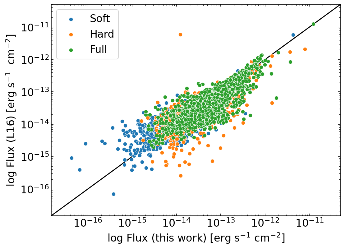
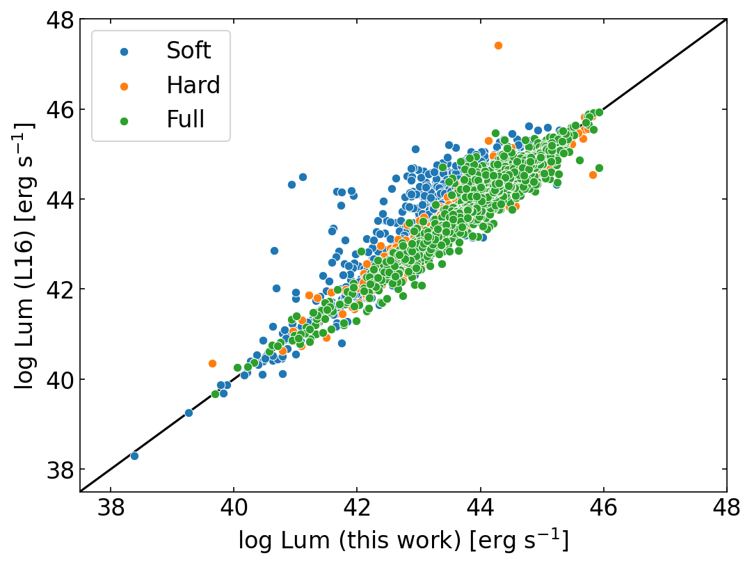
Figure 22: Comparison between derived fluxes (top panel) and observed luminosities (bottom panel) in this work and those from L16. Values are shown for the soft (blue), hard (orange), and full (green) bands. The black solid lines represent the one-to-one relation.

Appendix D XMM-Newton and Chandra selection functions

Figure 23 shows the simulations described in Section 5.1 for XMM-Newton (top panel, red scale) and Chandra (bottom panel, blue scale) individually. A qualitative comparison between the two panels immediately shows the different efficiencies in finding AGN. XMM-Newton is more effective than Chandra for almost all the parameter combinations. Only at low luminosity ($\log L_{\rm X}/\mathrm{erg\,\,s}^{-1}=43.5$), high redshift ($z>2$), and high absorption (log $\log N_{\rm H}/\mathrm{cm}^{-2}>23$—i.e. where it is more challenging to detect sources—the two telescopes are comparable, with a difference within $\sim$10-15%. The largest differences appear for high luminosity ($\log L_{\rm X}/\mathrm{erg\,\,s}^{-1}=45.5$) regimes, where XMM-Newton has an efficiency a factor up to $\sim$30-40 larger than Chandra. These differences are due to the combination of different effective areas and exposure times in the S82X, where XMM-Newton observations are overall deeper than most of the Chandra exposures.

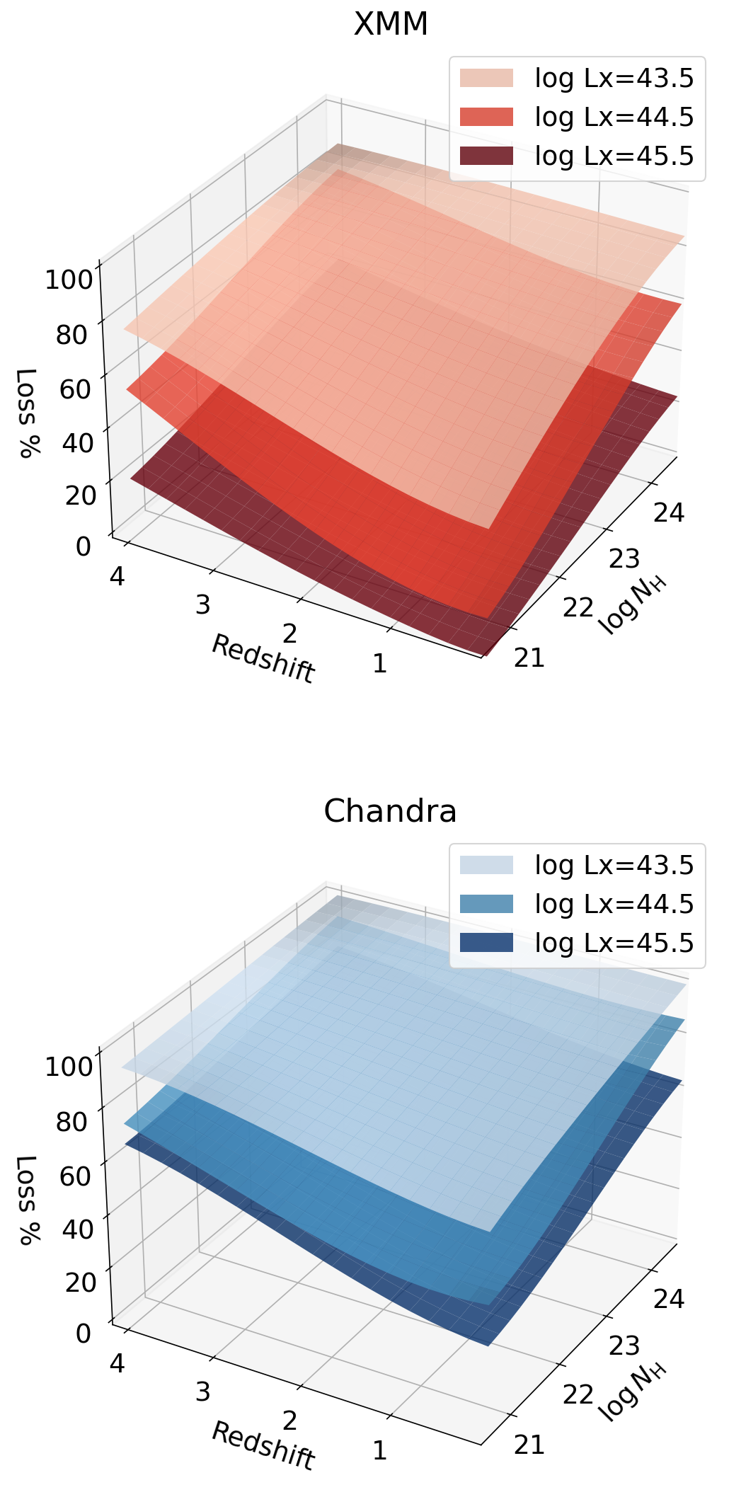
Figure 23: Loss surfaces for XMM-Newton (top, red) and Chandra (bottom, blue) as a function of $N_{\rm H}$ and redshifts, for different luminosity bins. Representative matrices for both the telescopes were applied.

References

- Aird et al. (2015) Aird, J., Coil, A. L., Georgakakis, A., et al. 2015, MNRAS, 451, 1892, doi: 10.1093/mnras/stv1062
- Aird et al. (2010) Aird, J., Nandra, K., Laird, E. S., et al. 2010, MNRAS, 401, 2531, doi: 10.1111/j.1365-2966.2009.15829.x
- Akaike (1974) Akaike, H. 1974, IEEE Transactions on Automatic Control, 19, 716, doi: 10.1109/TAC.1974.1100705
- Akylas & Georgantopoulos (2008) Akylas, A., & Georgantopoulos, I. 2008, A&A, 479, 735, doi: 10.1051/0004-6361:20077791
- Akylas et al. (2006) Akylas, A., Georgantopoulos, I., Georgakakis, A., Kitsionas, S., & Hatziminaoglou, E. 2006, A&A, 459, 693, doi: 10.1051/0004-6361:20054632
- Ananna et al. (2017) Ananna, T. T., Salvato, M., LaMassa, S., et al. 2017, ApJ, 850, 66, doi: 10.3847/1538-4357/aa937d
- Ananna et al. (2019) Ananna, T. T., Treister, E., Urry, C. M., et al. 2019, ApJ, 871, 240, doi: 10.3847/1538-4357/aafb77
- Ananna et al. (2022) Ananna, T. T., Weigel, A. K., Trakhtenbrot, B., et al. 2022, ApJS, 261, 9, doi: 10.3847/1538-4365/ac5b64
- Antonucci (1993) Antonucci, R. 1993, ARA&A, 31, 473, doi: 10.1146/annurev.aa.31.090193.002353
- Arnaud (1996) Arnaud, K. A. 1996, in Astronomical Society of the Pacific Conference Series, Vol. 101, Astronomical Data Analysis Software and Systems V, ed. G. H. Jacoby & J. Barnes, 17
- Astropy Collaboration et al. (2013) Astropy Collaboration, Robitaille, T. P., Tollerud, E. J., et al. 2013, A&A, 558, A33, doi: 10.1051/0004-6361/201322068
- Baldi et al. (2012) Baldi, A., Ettori, S., Molendi, S., et al. 2012, A&A, 537, A142, doi: 10.1051/0004-6361/201117836
- Ballantyne et al. (2011) Ballantyne, D. R., Draper, A. R., Madsen, K. K., Rigby, J. R., & Treister, E. 2011, ApJ, 736, 56, doi: 10.1088/0004-637X/736/1/56
- Baloković et al. (2021) Baloković, M., Cabral, S. E., Brenneman, L., & Urry, C. M. 2021, ApJ, 916, 90, doi: 10.3847/1538-4357/abff4d
- Baloković et al. (2018) Baloković, M., Brightman, M., Harrison, F. A., et al. 2018, ApJ, 854, 42, doi: 10.3847/1538-4357/aaa7eb
- Barchiesi et al. (2021) Barchiesi, L., Pozzi, F., Vignali, C., et al. 2021, PASA, 38, e033, doi: 10.1017/pasa.2021.26
- Barret et al. (2020) Barret, D., Decourchelle, A., Fabian, A., et al. 2020, Astronomische Nachrichten, 341, 224, doi: https://doi.org/10.1002/asna.202023782
- Bartalucci et al. (2014) Bartalucci, I., Mazzotta, P., Bourdin, H., & Vikhlinin, A. 2014, A&A, 566, A25, doi: 10.1051/0004-6361/201423443
- Blecha et al. (2018) Blecha, L., Snyder, G. F., Satyapal, S., & Ellison, S. L. 2018, MNRAS, 478, 3056, doi: 10.1093/mnras/sty1274
- Blustin et al. (2005) Blustin, A. J., Page, M. J., Fuerst, S. V., Branduardi-Raymont, G., & Ashton, C. E. 2005, A&A, 431, 111, doi: 10.1051/0004-6361:20041775
- Boissay et al. (2014) Boissay, R., Paltani, S., Ponti, G., et al. 2014, A&A, 567, A44, doi: 10.1051/0004-6361/201423494
- Bouwens et al. (2015) Bouwens, R. J., Illingworth, G. D., Oesch, P. A., et al. 2015, ApJ, 803, 34, doi: 10.1088/0004-637X/803/1/34
- Brandt & Alexander (2015) Brandt, W. N., & Alexander, D. M. 2015, A&A Rev., 23, 1, doi: 10.1007/s00159-014-0081-z
- Brightman et al. (2014) Brightman, M., Nandra, K., Salvato, M., et al. 2014, MNRAS, 443, 1999, doi: 10.1093/mnras/stu1175
- Brunner et al. (2022) Brunner, H., Liu, T., Lamer, G., et al. 2022, A&A, 661, A1, doi: 10.1051/0004-6361/202141266
- Buchner et al. (2014) Buchner, J., Georgakakis, A., Nandra, K., et al. 2014, A&A, 564, A125, doi: 10.1051/0004-6361/201322971
- Buchner et al. (2015) —. 2015, ApJ, 802, 89, doi: 10.1088/0004-637X/802/2/89
- Burnham & Anderson (2002) Burnham, K. P., & Anderson, D. R. 2002, Model selection and multimodel inference: a practical information-theoretic approach (Springer)
- Carilli & Walter (2013) Carilli, C. L., & Walter, F. 2013, ARA&A, 51, 105, doi: 10.1146/annurev-astro-082812-140953
- Cash (1979) Cash, W. 1979, ApJ, 228, 939, doi: 10.1086/156922
- Cavanaugh (1997) Cavanaugh, J. E. 1997, Statistics & Probability Letters, 33, 201, doi: https://doi.org/10.1016/S0167-7152(96)00128-9
- Chakraborty et al. (2021) Chakraborty, S., Ratheesh, A., Bhattacharyya, S., et al. 2021, MNRAS, 508, 475, doi: 10.1093/mnras/stab2530
- Chen (2017) Chen, Y.-C. 2017, Biostatistics & Epidemiology, 1, 161, doi: 10.1080/24709360.2017.1396742
- Civano et al. (2016) Civano, F., Marchesi, S., Comastri, A., et al. 2016, ApJ, 819, 62, doi: 10.3847/0004-637X/819/1/62
- Comastri et al. (1995) Comastri, A., Setti, G., Zamorani, G., & Hasinger, G. 1995, A&A, 296, 1. https://arxiv.org/abs/astro-ph/9409067
- Cowie et al. (2003) Cowie, L. L., Barger, A. J., Bautz, M. W., Brandt, W. N., & Garmire, G. P. 2003, ApJ, 584, L57, doi: 10.1086/368404
- Davies & Baddeley (2018) Davies, T. M., & Baddeley, A. 2018, Statistics and Computing, 28, 937, doi: 10.1007/s11222-017-9772-4
- De Luca & Molendi (2004) De Luca, A., & Molendi, S. 2004, A&A, 419, 837, doi: 10.1051/0004-6361:20034421
- Del Moro et al. (2013) Del Moro, A., Alexander, D. M., Mullaney, J. R., et al. 2013, A&A, 549, A59, doi: 10.1051/0004-6361/201219880
- Delvecchio et al. (2014) Delvecchio, I., Gruppioni, C., Pozzi, F., et al. 2014, MNRAS, 439, 2736, doi: 10.1093/mnras/stu130
- Delvecchio et al. (2017) Delvecchio, I., Smolčić, V., Zamorani, G., et al. 2017, A&A, 602, A3, doi: 10.1051/0004-6361/201629367
- Duras et al. (2020) Duras, F., Bongiorno, A., Ricci, F., et al. 2020, A&A, 636, A73, doi: 10.1051/0004-6361/201936817
- Eddington (1913) Eddington, A. S. 1913, MNRAS, 73, 359, doi: 10.1093/mnras/73.5.359
- Evans et al. (2010) Evans, I. N., Primini, F. A., Glotfelty, K. J., et al. 2010, ApJS, 189, 37, doi: 10.1088/0067-0049/189/1/37
- Feigelson & Babu (2012) Feigelson, E. D., & Babu, G. J. 2012, Modern Statistical Methods for Astronomy
- Fiore et al. (2012) Fiore, F., Puccetti, S., Grazian, A., et al. 2012, A&A, 537, A16, doi: 10.1051/0004-6361/201117581
- Foreman-Mackey et al. (2013) Foreman-Mackey, D., Hogg, D. W., Lang, D., & Goodman, J. 2013, PASP, 125, 306, doi: 10.1086/670067
- Freyberg et al. (2004) Freyberg, M. J., Briel, U. G., Dennerl, K., et al. 2004, in Society of Photo-Optical Instrumentation Engineers (SPIE) Conference Series, Vol. 5165, X-Ray and Gamma-Ray Instrumentation for Astronomy XIII, ed. K. A. Flanagan & O. H. W. Siegmund, 112–122, doi: 10.1117/12.506277
- Fruscione et al. (2006) Fruscione, A., McDowell, J. C., Allen, G. E., et al. 2006, in Society of Photo-Optical Instrumentation Engineers (SPIE) Conference Series, Vol. 6270, Society of Photo-Optical Instrumentation Engineers (SPIE) Conference Series, ed. D. R. Silva & R. E. Doxsey, 62701V, doi: 10.1117/12.671760
- Gabriel et al. (2004) Gabriel, C., Denby, M., Fyfe, D. J., et al. 2004, in Astronomical Society of the Pacific Conference Series, Vol. 314, Astronomical Data Analysis Software and Systems (ADASS) XIII, ed. F. Ochsenbein, M. G. Allen, & D. Egret, 759
- Gaskin et al. (2019) Gaskin, J. A., Swartz, D. A., Vikhlinin, A., et al. 2019, Journal of Astronomical Telescopes, Instruments, and Systems, 5, 021001, doi: 10.1117/1.JATIS.5.2.021001
- Gehrels (1986) Gehrels, N. 1986, ApJ, 303, 336, doi: 10.1086/164079
- Georgakakis et al. (2017) Georgakakis, A., Salvato, M., Liu, Z., et al. 2017, MNRAS, 469, 3232, doi: 10.1093/mnras/stx953
- Gierliński & Done (2004) Gierliński, M., & Done, C. 2004, MNRAS, 349, L7, doi: 10.1111/j.1365-2966.2004.07687.x
- Gilli et al. (2007) Gilli, R., Comastri, A., & Hasinger, G. 2007, A&A, 463, 79, doi: 10.1051/0004-6361:20066334
- Goodman & Weare (2010) Goodman, J., & Weare, J. 2010, Communications in Applied Mathematics and Computational Science, 5, 65, doi: 10.2140/camcos.2010.5.65
- Gordon & Arnaud (2021) Gordon, C., & Arnaud, K. 2021, PyXspec: Python interface to XSPEC spectral-fitting program. http://ascl.net/2101.014
- Hasinger (2008) Hasinger, G. 2008, A&A, 490, 905, doi: 10.1051/0004-6361:200809839
- Hatcher et al. (2021) Hatcher, C., Kirkpatrick, A., Fornasini, F., et al. 2021, AJ, 162, 65, doi: 10.3847/1538-3881/ac0530
- Hickox & Alexander (2018) Hickox, R. C., & Alexander, D. M. 2018, ARA&A, 56, 625, doi: 10.1146/annurev-astro-081817-051803
- Hönig & Beckert (2007) Hönig, S. F., & Beckert, T. 2007, MNRAS, 380, 1172, doi: 10.1111/j.1365-2966.2007.12157.x
- Hopkins & Hernquist (2009) Hopkins, P. F., & Hernquist, L. 2009, ApJ, 694, 599, doi: 10.1088/0004-637X/694/1/599
- Hopkins et al. (2005) Hopkins, P. F., Hernquist, L., Cox, T. J., et al. 2005, ApJ, 630, 716, doi: 10.1086/432463
- Hopkins et al. (2006) —. 2006, ApJS, 163, 1, doi: 10.1086/499298
- Hopkins et al. (2008) Hopkins, P. F., Hernquist, L., Cox, T. J., & Kereš, D. 2008, ApJS, 175, 356, doi: 10.1086/524362
- Hopkins et al. (2007) Hopkins, P. F., Hernquist, L., Cox, T. J., Robertson, B., & Krause, E. 2007, ApJ, 669, 45, doi: 10.1086/521590
- Hunter (2007) Hunter, J. D. 2007, Computing in Science & Engineering, 9, 90, doi: 10.1109/MCSE.2007.55
- Iwasawa et al. (2011) Iwasawa, K., Sanders, D. B., Teng, S. H., et al. 2011, A&A, 529, A106, doi: 10.1051/0004-6361/201015264
- Iwasawa et al. (2012) Iwasawa, K., Gilli, R., Vignali, C., et al. 2012, A&A, 546, A84, doi: 10.1051/0004-6361/201220036
- Iwasawa et al. (2020) Iwasawa, K., Comastri, A., Vignali, C., et al. 2020, arXiv e-prints, arXiv:2004.07604. https://arxiv.org/abs/2004.07604
- Kalberla et al. (2005) Kalberla, P. M. W., Burton, W. B., Hartmann, D., et al. 2005, A&A, 440, 775, doi: 10.1051/0004-6361:20041864
- Kass & Raftery (1995) Kass, R. E., & Raftery, A. E. 1995, Journal of the American Statistical Association, 90, 773, doi: 10.1080/01621459.1995.10476572
- Koss et al. (2022) Koss, M. J., Trakhtenbrot, B., Ricci, C., et al. 2022, arXiv e-prints, arXiv:2207.12428. https://arxiv.org/abs/2207.12428
- Kuntz & Snowden (2000) Kuntz, K. D., & Snowden, S. L. 2000, ApJ, 543, 195, doi: 10.1086/317071
- LaMassa et al. (2019a) LaMassa, S. M., Georgakakis, A., Vivek, M., et al. 2019a, ApJ, 876, 50, doi: 10.3847/1538-4357/ab108b
- LaMassa et al. (2019b) LaMassa, S. M., Yaqoob, T., Boorman, P. G., et al. 2019b, ApJ, 887, 173, doi: 10.3847/1538-4357/ab552c
- LaMassa et al. (2014) LaMassa, S. M., Yaqoob, T., Ptak, A. F., et al. 2014, ApJ, 787, 61, doi: 10.1088/0004-637X/787/1/61
- LaMassa et al. (2013a) LaMassa, S. M., Urry, C. M., Glikman, E., et al. 2013a, MNRAS, 432, 1351, doi: 10.1093/mnras/stt553
- LaMassa et al. (2013b) LaMassa, S. M., Urry, C. M., Cappelluti, N., et al. 2013b, MNRAS, 436, 3581, doi: 10.1093/mnras/stt1837
- LaMassa et al. (2016) —. 2016, ApJ, 817, 172, doi: 10.3847/0004-637X/817/2/172
- Lanzuisi et al. (2013) Lanzuisi, G., Civano, F., Elvis, M., et al. 2013, MNRAS, 431, 978, doi: 10.1093/mnras/stt222
- Lanzuisi et al. (2015) Lanzuisi, G., Ranalli, P., Georgantopoulos, I., et al. 2015, A&A, 573, A137, doi: 10.1051/0004-6361/201424924
- Lawrence (1991) Lawrence, A. 1991, MNRAS, 252, 586, doi: 10.1093/mnras/252.4.586
- Leccardi & Molendi (2008) Leccardi, A., & Molendi, S. 2008, A&A, 487, 461, doi: 10.1051/0004-6361:200810113
- Liddle (2007) Liddle, A. R. 2007, MNRAS, 377, L74, doi: 10.1111/j.1745-3933.2007.00306.x
- Liu et al. (2017) Liu, T., Tozzi, P., Wang, J.-X., et al. 2017, ApJS, 232, 8, doi: 10.3847/1538-4365/aa7847
- Liu et al. (2016) Liu, Z., Merloni, A., Georgakakis, A., et al. 2016, MNRAS, 459, 1602, doi: 10.1093/mnras/stw753
- Luo et al. (2017) Luo, B., Brandt, W. N., Xue, Y. Q., et al. 2017, ApJS, 228, 2, doi: 10.3847/1538-4365/228/1/2
- Lusso et al. (2012) Lusso, E., Comastri, A., Simmons, B. D., et al. 2012, MNRAS, 425, 623, doi: 10.1111/j.1365-2966.2012.21513.x
- Lynden-Bell (1971) Lynden-Bell, D. 1971, MNRAS, 155, 95, doi: 10.1093/mnras/155.1.95
- Madau & Dickinson (2014) Madau, P., & Dickinson, M. 2014, ARA&A, 52, 415, doi: 10.1146/annurev-astro-081811-125615
- Magdziarz & Zdziarski (1995) Magdziarz, P., & Zdziarski, A. A. 1995, MNRAS, 273, 837, doi: 10.1093/mnras/273.3.837
- Marchesi et al. (2019) Marchesi, S., Ajello, M., Zhao, X., et al. 2019, ApJ, 882, 162, doi: 10.3847/1538-4357/ab340a
- Marchesi et al. (2016) Marchesi, S., Lanzuisi, G., Civano, F., et al. 2016, ApJ, 830, 100, doi: 10.3847/0004-637X/830/2/100
- Marchesi et al. (2020) Marchesi, S., Gilli, R., Lanzuisi, G., et al. 2020, A&A, 642, A184, doi: 10.1051/0004-6361/202038622
- Masini et al. (2020) Masini, A., Hickox, R. C., Carroll, C. M., et al. 2020, ApJS, 251, 2, doi: 10.3847/1538-4365/abb607
- Mateos et al. (2017) Mateos, S., Carrera, F. J., Barcons, X., et al. 2017, ApJ, 841, L18, doi: 10.3847/2041-8213/aa7268
- Matt & Iwasawa (2019) Matt, G., & Iwasawa, K. 2019, MNRAS, 482, 151, doi: 10.1093/mnras/sty2697
- Merloni et al. (2012) Merloni, A., Predehl, P., Becker, W., et al. 2012, arXiv e-prints, arXiv:1209.3114. https://arxiv.org/abs/1209.3114
- Miyaji et al. (2000) Miyaji, T., Hasinger, G., & Schmidt, M. 2000, A&A, 353, 25. https://arxiv.org/abs/astro-ph/9910410
- Miyaji et al. (2001) —. 2001, A&A, 369, 49, doi: 10.1051/0004-6361:20010102
- Miyaji et al. (2015) Miyaji, T., Hasinger, G., Salvato, M., et al. 2015, ApJ, 804, 104, doi: 10.1088/0004-637X/804/2/104
- Mountrichas et al. (2020) Mountrichas, G., Georgantopoulos, I., Ruiz, A., & Kampylis, G. 2020, MNRAS, 491, 1727, doi: 10.1093/mnras/stz3076
- Murphy & Yaqoob (2009) Murphy, K. D., & Yaqoob, T. 2009, MNRAS, 397, 1549, doi: 10.1111/j.1365-2966.2009.15025.x
- Mushotzky et al. (2019) Mushotzky, R., Aird, J., Barger, A. J., et al. 2019, in BAAS, Vol. 51, 107. https://arxiv.org/abs/1903.04083
- Nandra & Pounds (1994) Nandra, K., & Pounds, K. A. 1994, MNRAS, 268, 405, doi: 10.1093/mnras/268.2.405
- Nanni et al. (2020) Nanni, R., Gilli, R., Vignali, C., et al. 2020, arXiv e-prints, arXiv:2003.13710. https://arxiv.org/abs/2003.13710
- Padovani et al. (2017) Padovani, P., Alexander, D. M., Assef, R. J., et al. 2017, A&A Rev., 25, 2, doi: 10.1007/s00159-017-0102-9
- Page & Carrera (2000) Page, M. J., & Carrera, F. J. 2000, MNRAS, 311, 433, doi: 10.1046/j.1365-8711.2000.03105.x
- Park et al. (2006) Park, T., Kashyap, V. L., Siemiginowska, A., et al. 2006, ApJ, 652, 610, doi: 10.1086/507406
- Peca et al. (2021) Peca, A., Vignali, C., Gilli, R., et al. 2021, ApJ, 906, 90, doi: 10.3847/1538-4357/abc9c7
- Piconcelli et al. (2005) Piconcelli, E., Jimenez-Bailón, E., Guainazzi, M., et al. 2005, A&A, 432, 15, doi: 10.1051/0004-6361:20041621
- Pierre et al. (2016) Pierre, M., Pacaud, F., Adami, C., et al. 2016, A&A, 592, A1, doi: 10.1051/0004-6361/201526766
- Predehl et al. (2021) Predehl, P., Andritschke, R., Arefiev, V., et al. 2021, A&A, 647, A1, doi: 10.1051/0004-6361/202039313
- Ranalli et al. (2013) Ranalli, P., Comastri, A., Vignali, C., et al. 2013, A&A, 555, A42, doi: 10.1051/0004-6361/201321211
- Ricci et al. (2017a) Ricci, C., Trakhtenbrot, B., Koss, M. J., et al. 2017a, ApJS, 233, 17, doi: 10.3847/1538-4365/aa96ad
- Ricci et al. (2017b) Ricci, C., Bauer, F. E., Treister, E., et al. 2017b, MNRAS, 468, 1273, doi: 10.1093/mnras/stx173
- Salvato et al. (2009) Salvato, M., Hasinger, G., Ilbert, O., et al. 2009, ApJ, 690, 1250, doi: 10.1088/0004-637X/690/2/1250
- Sanders et al. (1988) Sanders, D. B., Soifer, B. T., Elias, J. H., et al. 1988, ApJ, 325, 74, doi: 10.1086/165983
- Schmidt (1968) Schmidt, M. 1968, ApJ, 151, 393, doi: 10.1086/149446
- Schwarz (1978) Schwarz, G. 1978, The Annals of Statistics, 6, 461 , doi: 10.1214/aos/1176344136
- Shemmer et al. (2006) Shemmer, O., Brandt, W. N., Netzer, H., Maiolino, R., & Kaspi, S. 2006, ApJ, 646, L29, doi: 10.1086/506911
- Sijacki et al. (2015) Sijacki, D., Vogelsberger, M., Genel, S., et al. 2015, MNRAS, 452, 575, doi: 10.1093/mnras/stv1340
- Simpson (2005) Simpson, C. 2005, MNRAS, 360, 565, doi: 10.1111/j.1365-2966.2005.09043.x
- Soltan (1982) Soltan, A. 1982, MNRAS, 200, 115, doi: 10.1093/mnras/200.1.115
- Somerville et al. (2008) Somerville, R. S., Hopkins, P. F., Cox, T. J., Robertson, B. E., & Hernquist, L. 2008, MNRAS, 391, 481, doi: 10.1111/j.1365-2966.2008.13805.x
- Suchy et al. (2012) Suchy, S., Fürst, F., Pottschmidt, K., et al. 2012, ApJ, 745, 124, doi: 10.1088/0004-637X/745/2/124
- Taylor (2005) Taylor, M. B. 2005, in Astronomical Society of the Pacific Conference Series, Vol. 347, Astronomical Data Analysis Software and Systems XIV, ed. P. Shopbell, M. Britton, & R. Ebert, 29
- Treister et al. (2010) Treister, E., Natarajan, P., Sanders, D. B., et al. 2010, Science, 328, 600, doi: 10.1126/science.1184246
- Treister et al. (2012) Treister, E., Schawinski, K., Urry, C. M., & Simmons, B. D. 2012, ApJ, 758, L39, doi: 10.1088/2041-8205/758/2/L39
- Treister & Urry (2006) Treister, E., & Urry, C. M. 2006, ApJ, 652, L79, doi: 10.1086/510237
- Treister et al. (2009) Treister, E., Urry, C. M., & Virani, S. 2009, ApJ, 696, 110, doi: 10.1088/0004-637X/696/1/110
- Treister et al. (2004) Treister, E., Urry, C. M., Chatzichristou, E., et al. 2004, ApJ, 616, 123, doi: 10.1086/424891
- Ueda et al. (2014) Ueda, Y., Akiyama, M., Hasinger, G., Miyaji, T., & Watson, M. G. 2014, ApJ, 786, 104, doi: 10.1088/0004-637X/786/2/104
- Ueda et al. (2003) Ueda, Y., Akiyama, M., Ohta, K., & Miyaji, T. 2003, ApJ, 598, 886, doi: 10.1086/378940
- Ueda et al. (2007) Ueda, Y., Eguchi, S., Terashima, Y., et al. 2007, ApJ, 664, L79, doi: 10.1086/520576
- Urry & Padovani (1995) Urry, C. M., & Padovani, P. 1995, PASP, 107, 803, doi: 10.1086/133630
- Vasudevan et al. (2014) Vasudevan, R. V., Mushotzky, R. F., Reynolds, C. S., et al. 2014, ApJ, 785, 30, doi: 10.1088/0004-637X/785/1/30
- Vito et al. (2014) Vito, F., Gilli, R., Vignali, C., et al. 2014, MNRAS, 445, 3557, doi: 10.1093/mnras/stu2004
- Vito et al. (2018) Vito, F., Brandt, W. N., Yang, G., et al. 2018, MNRAS, 473, 2378, doi: 10.1093/mnras/stx2486
- Vito et al. (2019) Vito, F., Brandt, W. N., Bauer, F. E., et al. 2019, A&A, 630, A118, doi: 10.1051/0004-6361/201936217
- Volonteri et al. (2016) Volonteri, M., Dubois, Y., Pichon, C., & Devriendt, J. 2016, MNRAS, 460, 2979, doi: 10.1093/mnras/stw1123
- Wasserman (2006) Wasserman, L. 2006, All of Nonparametric Statistics (New York, NY: Springer New York), 125–144, doi: 10.1007/0-387-30623-4_6
- Yaqoob (2012) Yaqoob, T. 2012, MNRAS, 423, 3360, doi: 10.1111/j.1365-2966.2012.21129.x
- Yuan et al. (2020) Yuan, Z., Jarvis, M. J., & Wang, J. 2020, ApJS, 248, 1, doi: 10.3847/1538-4365/ab855b
- Yuan et al. (2022) Yuan, Z., Zhang, X., Wang, J., Cheng, X., & Wang, W. 2022, ApJS, 260, 10, doi: 10.3847/1538-4365/ac596a