HashFormers: Towards Vocabulary-independent Pre-trained Transformers

Abstract

Transformer-based pre-trained language models are vocabulary-dependent, mapping by default each token to its corresponding embedding. This one-to-one mapping results into embedding matrices that occupy a lot of memory (i.e. millions of parameters) and grow linearly with the size of the vocabulary. Previous work on on-device transformers dynamically generate token embeddings on-the-fly without embedding matrices using locality-sensitive hashing over morphological information. These embeddings are subsequently fed into transformer layers for text classification. However, these methods are not pre-trained. Inspired by this line of work, we propose HashFormers, a new family of vocabulary-independent pre-trained transformers that support an unlimited vocabulary (i.e. all possible tokens in a corpus) given a substantially smaller fixed-sized embedding matrix. We achieve this by first introducing computationally cheap hashing functions that bucket together individual tokens to embeddings. We also propose three variants that do not require an embedding matrix at all, further reducing the memory requirements. We empirically demonstrate that HashFormers are more memory efficient compared to standard pre-trained transformers while achieving comparable predictive performance when fine-tuned on multiple text classification tasks. For example, our most efficient HashFormer variant has a negligible performance degradation (0.4% on GLUE) using only 99.1K parameters for representing the embeddings compared to 12.3-38M parameters of state-of-the-art models.

1 Introduction

The majority of transformer-based (Vaswani et al., 2017) pre-trained language models (PLMs; Devlin et al. 2019; Liu et al. 2019; Dai et al. 2019; Yang et al. 2019) are vocabulary-dependent, with each single token mapped to its corresponding vector in an embedding matrix. This one-to-one mapping makes it impractical to support out-of-vocabulary tokens such as misspellings or rare words (Pruthi et al., 2019; Sun et al., 2020). Moreover, it linearly increases the memory requirements with the vocabulary size for the token embedding matrix (Chung et al., 2021). For example, given a token embedding size of 768, BERT-base with a vocabulary of 30.5K tokens needs 23.4M out of 110M total parameters while RoBERTa-base with 50K tokens needs 38M out of 125M total parameters. Hence, disentangling the design of PLMs from the vocabulary size and tokenization approaches would inherently improve memory efficiency and pre-training, especially for researchers with access to limited computing resources (Strubell et al., 2019; Schwartz et al., 2020).

Previous efforts for making transformer-based models vocabulary-independent include dynamically generating token embeddings on-the-fly without embedding matrices using hash embeddings (Svenstrup et al., 2017; Ravi, 2019) over morphological information Sankar et al. (2021a). However, these embeddings are subsequently fed into transformer layers trained from scratch for on-device text classification without any pre-training. Clark et al. (2022) proposed CANINE, a model that operates on Unicode characters using a low-collision multi-hashing strategy to support ~1.1M Unicode codepoints as well as infinite character four-grams. This makes CANINE independent of tokenization while limiting the parameters of its embedding layer to 12.3M. Xue et al. (2022) proposed models that take as input byte sequences representing characters without explicit tokenization or a predefined vocabulary to pre-train transformers in multilingual settings.

In this paper, we propose HashFormers a new family of vocabulary-independent PLMs. Our models support an unlimited vocabulary (i.e. all possible tokens in a given pre-training corpus) with a considerably smaller fixed-sized embedding matrix. We achieve this by employing simple yet computationally efficient hashing functions that bucket together individual tokens to embeddings inspired by the hash embedding methods of Svenstrup et al. (2017) and Sankar et al. (2021a). Our contributions are as follows:

1. To the best of our knowledge, this is the first attempt towards reducing memory requirements of PLMs using various hash embeddings with different hash strategies aiming to substantially reduce the embedding matrix compared to the vocabulary size;

2. Three HashFormer variants further reduce the memory footprint by entirely removing the need of an embedding matrix;

3. We empirically demonstrate that our HashFormers are consistently more memory efficient compared to vocabulary-dependent PLMs while achieving comparable predictive performance when fine-tuned on a battery of standard text classification tasks.

2 Related Work

2.1 Tokenization and Vocabulary-independent Transformers

Typically, PLMs are pre-trained on text that has been tokenized using subword tokenization techniques such as WordPiece (Wu et al., 2016), Byte-Pair-Encoding (BPE; Sennrich et al. 2016) and SentencePiece (Kudo and Richardson, 2018).

Attempts to remove the dependency of PLMs on a separate tokenization component include models that directly operate on sequences of characters (Tay et al., 2022; El Boukkouri et al., 2020). However, these approaches do not remove the requirement of an embedding matrix. Recently, Xue et al. (2022) proposed PLMs that take as input byte sequences representing characters without explicit tokenization or a predefined vocabulary in multilingual settings. PLMs in Clark et al. (2022) operating on Unicode characters or ngrams also achieved the similar goal. These methods improve memory efficiency but still rely on a complex process to encode the relatively long ngram sequences of extremely long byte/Unicode sequences, affecting their computational efficiency.

In a different direction, Sankar et al. (2021b) proposed ProFormer, an on-device vocabulary-independent transformer-based model. It generates token hash embeddings (Svenstrup et al., 2017; Shi et al., 2009; Ganchev and Dredze, 2008) on-the-fly by applying locality-sensitive hashing over morphological features. Subsequently, hash embeddings are fed to transformer layers for text classification. However, ProFormer is trained from scratch using task-specific data without any pre-training.

2.2 Compressing PLM Embeddings

A different line of work has focused on compressing the embedding matrix in transformer models (Ganesh et al., 2021). Prakash et al. (2020) proposed to use compositional code embeddings (Shu and Nakayama, 2018) to reduce the size of the embeddings in PLMs for semantic parsing. Zhao et al. (2021) developed a distillation method to align teacher and student token embeddings using a mixed-vocabulary training (i.e. the student and teacher models have different vocabularies) for learning smaller BERT models. However, these approaches still rely on a predefined vocabulary. Clark et al. (2022) adopted low-collision multi-hashing strategy to support ~1.1M Unicode codepoints and a larger space of character four-grams with a relatively small embedding matrix containing 12.3M parameters.

3 HashFormers

In this section, we present HashFormers, a family of vocabulary-independent hashing-based pre-trained transformers.

3.1 Many-to-One Mapping from Tokens to an Embedding

Given a token $t$, HashFormers use a hash function $\mathcal{H}$ to map $t$ into a value $v$. Using hashing allows our model to map many tokens into a single embedding and support an infinite vocabulary. We obtain the embedding index by squashing its hash value $v$ into $i=[1,...,N]$ where $\mathbf{e}=\mathbf{E}_{i}$ is the corresponding embedding from a matrix $\mathbf{E}\in\mathbb{R}^{N\times d}$ where $N$ is the number of the embeddings and $d$ is their dimensionality. We assume that $|V|\gg N$ where $|V|$ is the size of the vocabulary. Subsequently, $\mathbf{e}$ is passed through a series of transformer layers for pre-training. This is our first variant, HashFormer-Emb that relies on a look-up embedding matrix (see Figure 1). Our method is independent of tokenization choices.

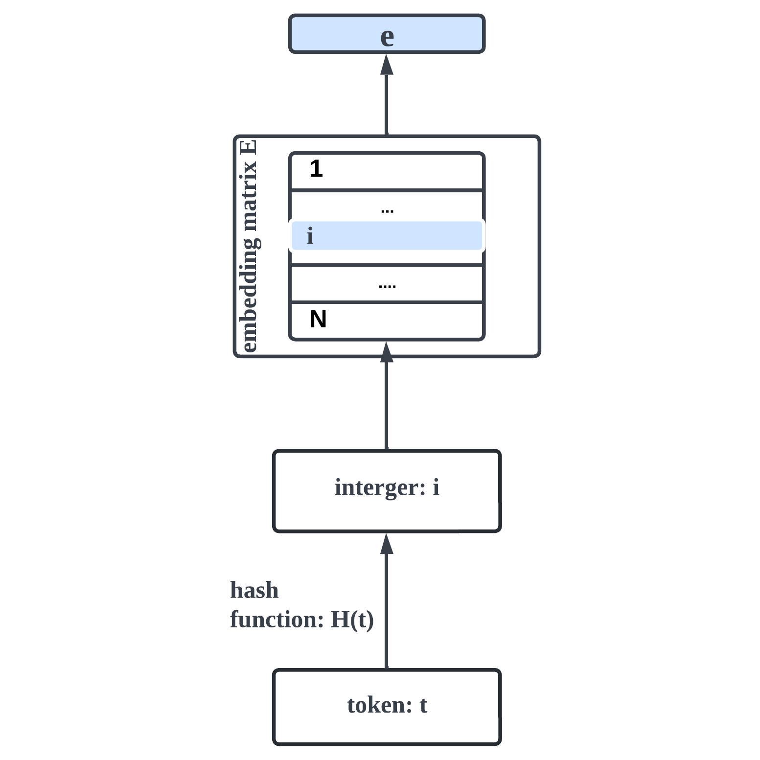
Figure 1: HashFormer-Emb.

3.2 Message-Direct Hashing (HashFormers-MD)

Our first approach to hash tokens is by using a Message-Digest (MD5) hash function (Rivest and Dusse, 1992) to map each token to its 128-bits output, $v=\mathcal{H}(t)$. The mapping can be reproduced given the same secret key. MD5 is a ‘random’ hashing approach, returning mostly different hashes for tokens with morphological or semantic similarities. For example:

$$\text{MD5}(\text{`play'}) =\textit{d077f244def8a70e5ea758bd8352fcd8}$$

$$\text{MD5}(\text{`plays'}) =\textit{4a258d930b7d3409982d727ddbb4ba88}$$

It is simple and does not require any pre-processing to obtain the bit encoding for each token. To map the hash output $v$ into its corresponding embedding, we transform its binary value into decimal and then compute the index $i$ to $\mathbf{E}$ as $i=v\mathbin{\%}N$.

3.3 Locality-Sensitive Hashing (HashFormers-LSH)

Locality-sensitive hashing (LSH) hashes similar tokens into the same indices with high probability (Rajaraman and Ullman, 2011). HashFormer-LSH uses LSH hashing to assign tokens with similar morphology (e.g. ‘play’, ‘plays’, ‘played’) to the same hash encoding. This requires an additional feature extraction step for token representation.

Token to Morphological Feature Vector:

We want to represent each token with a vector $\mathbf{x}$ as a bag of morphological (i.e. character n-grams) features. For each token, we first extract character n-grams ($n\in{1,2,3,4}$) to get a feature vector whose dimension is equal to the vocabulary size. Each element in the feature vector is weighted by the frequency of the character n-grams of the token.

Morphological Vector to Hash Index:

Once we obtain the morphological feature vector of each token, we first define $N$ random hyperplanes, each represented by a random unit vector $\mathbf{r^{i}}\in\mathbb{R}^{d_{x}}$, where $d_{x}$ is the dimensionality of the morphological feature vector. Following a similar approach to Kitaev et al. (2020), we compute the hash value $v$ as the index of the nearest random hyperplane vector to the token’s feature vector, $\mathbf{x}$ obtained by computing $v=\mathcal{H}(\mathbf{x})=\operatorname*{arg\,max}(\mathbf{x}\mathbf{R}),\mathbf{R}=[\mathbf{r}^{1};...;\mathbf{r}^{N}]$ where $[\alpha;\beta]$ denotes the concatenation of two vectors. This approach results into bucketing together tokens with similar morphological vectors. Similar to HashFormer-MD-Emb, we compute the embedding index as $i=v\mathbin{\%}N$.

To prevent storing a large projection matrix ($\mathbb{R}^{d_{x}\times N}$) for accommodating each unit vector, we design an on-the-fly computational approach. We only store a vector $\mathbf{\eta}\in\mathbb{R}^{d_{x}}$ that is randomly initialized from the standard normal distribution, guaranteeing that each column $\mathbf{r}$ in the matrix $\mathbf{R}$ is a permutation of $\mathbf{\eta}$ with a unique offset value (e.g. $\mathbf{r}^{1}=[\mathbf{\eta}_{2},...,\mathbf{\eta}_{N},\mathbf{\eta}_{1}]$). Each offset value only relies on the index of the hyperplane. This setting ensures that each hyperplane has the same L2-norm.

3.4 Compressing the Embedding Space

We also propose three embedding compression approaches that allow an even smaller number of parameters to represent token embeddings and support unlimited tokens (i.e. very large $|V|$) without forcing a large number of tokens to share the same embedding. For this purpose, we first use a hash function $\mathcal{H}$ to map each token $t$ into a $T$-bit value $b$, $b\in[0,2^{T})$. Then, we pass $b$ through a transformation procedure to generate the corresponding embedding (to facilitate computation, we cast $b$ into a $T$-bit vector $\mathbf{\tau}$). This way tokens with different values $b$ will be assigned to a different embedding by keeping the number of parameters relatively small. Figure 2 shows an overview of this method.

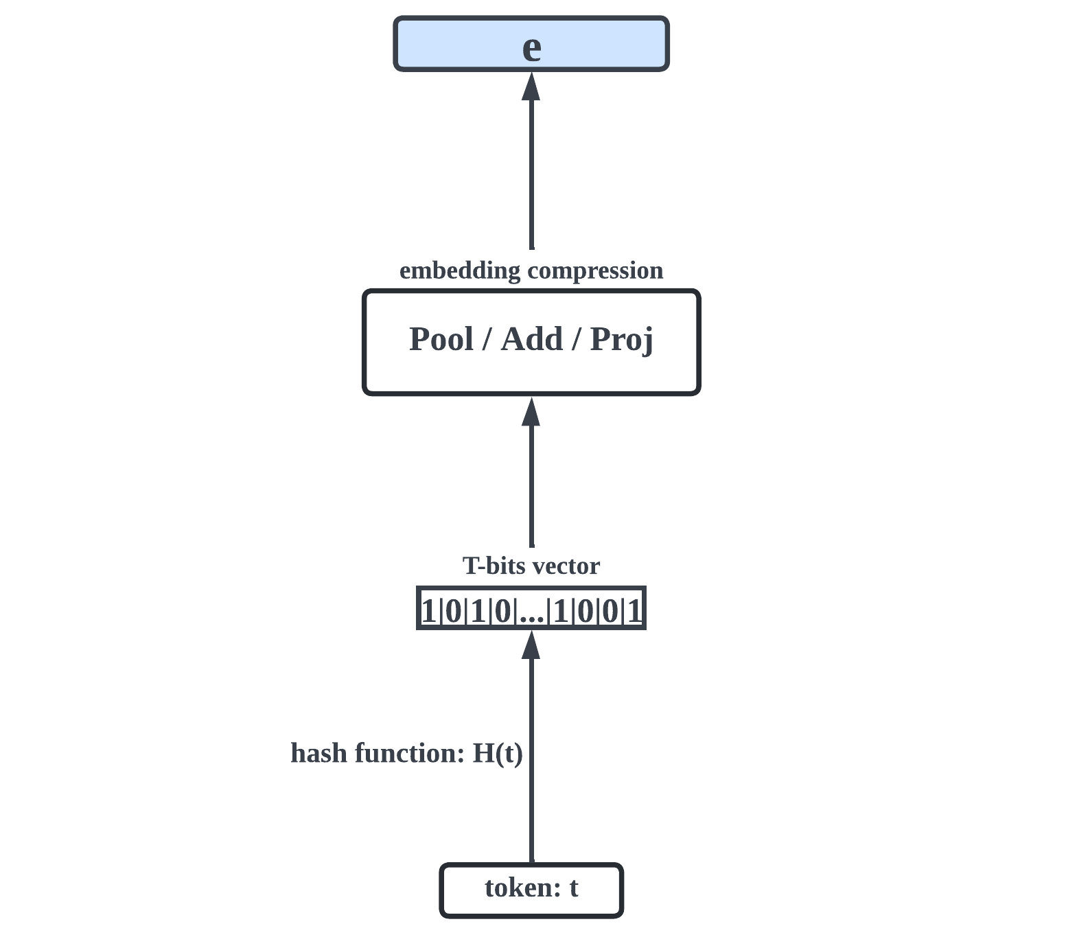
Figure 2: Compressing the embedding space.

Pooling Approach (Pool)

Inspired by Svenstrup et al. (2017) and Prakash et al. (2020), we first create a universal learnable codebook, which is a matrix denoted as $\mathbf{B}\in\mathbb{R}^{2^{k}\times d}$. Then, we split the hash bit vector $\tau$ in $k$ successive bits without overlap to obtain $\lceil\frac{T}{k}\rceil$ binary values. We then cast these binary values into an integer value representing a codeword. Hence, each token is represented by a vector $\mathbf{c}\in\mathbb{R}^{d}$ with elements $c_{j}\in[0,2^{k})$. For example, given $k=4$ and a 12-bits vector [1,0,1,0,0,1,0,0,0,0,0,1], 4-bit parts are treated as separate binary codewords [1010,0100,0001] then transformed into their decimal format codebook [10,4,1]. We construct the embedding $\mathbf{e}\in\mathbb{R}^{d}$ for each token by looking up the decimal codebook and extracting $\lceil\frac{T}{k}\rceil$ vectors corresponding to its $\lceil\frac{T}{k}\rceil$ codewords. We then apply a weighted average pooling on them using a softmax function:

$$\hat{\textbf{W}_{j}} =\frac{\exp\textbf{W}_{j}}{\sum_{l=1}^{\lceil\frac{T}{k}\rceil}\exp\textbf{W}_{l}},j=1,..,\lceil\tfrac{T}{k}\rceil$$ (1a)

$$\mathbf{e} =\sum_{j=1}^{\lceil\frac{T}{k}\rceil}[\mathbf{B}_{\mathbf{c}}\odot\hat{\textbf{W}}]_{j}$$ (1b)

where $\mathbf{W}\in\mathbb{R}^{\lceil\frac{T}{k}\rceil\times d}$ is a learnable weight matrix as well as the codebook $\mathbf{B}$. The total number of parameters required for this pooling transformation is $(\lceil\frac{T}{k}\rceil+2^{k})\times d$. This can be much smaller than the $N\times d$ parameters required for standard PLMs that use a one-to-one mapping between tokens and embeddings, where $N=|V|\gg(\lceil\frac{T}{k}\rceil+2^{k})$. Figure 3 shows the overview of the Pool process.

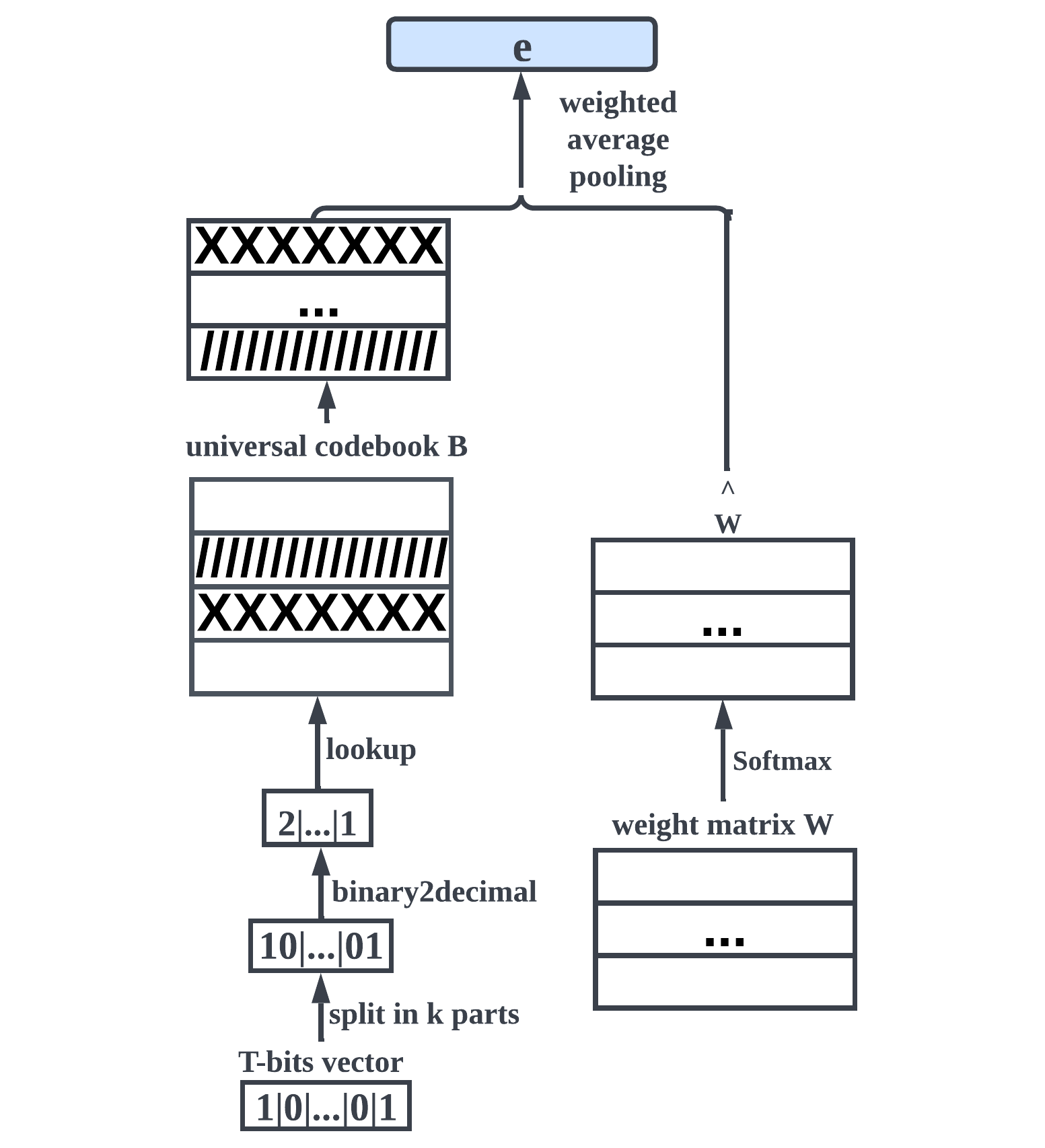
Figure 3: HashFormer-Pool.

Additive Approach (Add)

Different to the Pool method that uses a universal codebook, we create $T$ different codebooks $\{\textbf{B}^{1},\textbf{B}^{2},...,\textbf{B}^{T}\}$, each containing two learnable embedding vectors corresponding to codewords $0$ and $1$ respectively. We get a $T$-bits vector $\mathbf{\tau}\in\{0,1\}^{T}$ for each token, where each element in the vector $\mathbf{\tau}$ is treated as a codeword. We look up each codeword in their corresponding codebook to obtain $T$ vectors and add up them to compute the token embedding $\mathbf{e}$:

$$\mathbf{e}=\sum^{T}_{j=1}\textbf{B}^{j}_{\mathbf{\tau}_{j}}\bigg{/}\gamma$$ (2)

where $\mathbf{B}^{j}\in\mathbb{R}^{2\times d},j=1,..,T$, $\gamma$ is the scaling factor. Hence, the total number of parameters the additive transformation approach requires is $2\times T\times d$. Similar to the Pool approach, the number of parameters required is smaller than the vocabulary size: $2\times T\times d\ll N=|V|$.

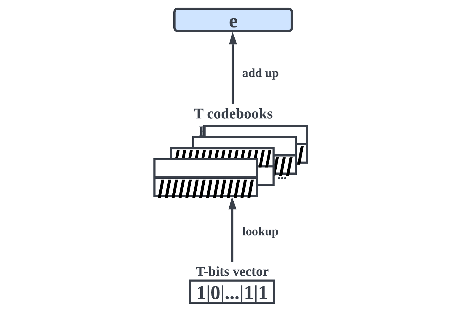
Figure 4: HashFormer-Add.

Projection Approach (Proj)

Finally, we propose a new simpler approach compared to Pool and Add. We create $T$ learnable random initialized vectors as $T$ pseudo-axes to trace the orientation of each $T$-bits vector $\mathbf{\tau}$ corresponding to the token $t$. Given a token bit vector $\mathbf{\tau}$, the $j$^th element in the embedding $\mathbf{e}$ is computed as the Pearson’s correlation coefficient (PCC) between $\mathbf{\tau}$ and the learnable vector $\mathbf{w}^{j}$ corresponding to $j$.

$$\mathbf{e}_{j} =\frac{\langle\mathbf{\tau}-\bar{\tau},\mathbf{w^{j}}-\bar{\mathbf{w^{j}}}\rangle}{\|\tau-\bar{\tau}\|\centerdot\|\mathbf{w^{j}}-\bar{\mathbf{w^{j}}}\|},\quad j=1,...,d$$ (3)

$$\mathbf{e} =(e_{1},...,e_{d})$$

$\mathbf{w}^{j}\in\mathbb{R}^{d},j=1,..,T$, hence, the total number of parameters the projection transformation approach requires is only $T\times d\ll N=|V|$. Figure 5 depicts an overview of our HashFormer-Proj model.

3.5 Hashing for Compressed Embeddings

Similar to the embedding based HashFormers-Emb, our embedding compression-based models also consider the same two hash approaches (MD and LSH) for generating the $T$-bit vector of each token.

MD5:

We directly map the tokens to its 128-bits output $b$ with a universal secret key.

LSH:

We repeat the same morphological feature extraction step to obtain a feature vector $\mathbf{x}$ corresponding to each token $t$. However, rather than using $2^{T}$ random hyperplanes that require storing vectors of size $\mathbb{R}^{2^{T}}$, we simply use $T$ random hyperplanes similar to  Ravi (2019); Sankar et al. (2021b). Each bit in $b$ represents which side of the corresponding hyperplane $\mathbf{r}\in\mathbb{R}^{d}$ the feature vector $\mathbf{x}$ is located: $b_{j}=\operatorname{sgn}(\operatorname{sgn}(\mathbf{x}\cdot\mathbf{r^{i}})+1),j=1,...,T$. This allows an on-the-fly computation without storing any vector (Ravi, 2019).

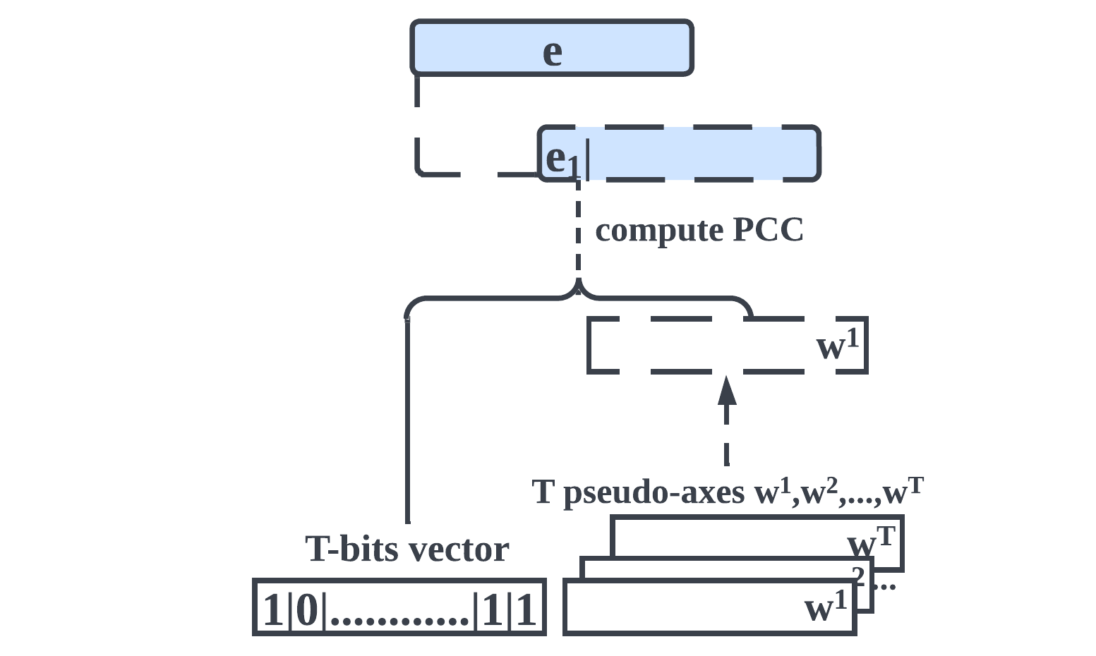
Figure 5: HashFormer-Proj.

3.6 Pre-training Objective

Since our models support an arbitrary number of unique tokens, it is intractable to use a standard Masked Language Modeling (Devlin et al., 2019) pre-training objective. We opted using Shuffle + Random (S+R), a computationally efficient three-way classification objective introduced by Yamaguchi et al. (2021) for predicting whether tokens in the input have been shuffled, replaced with random tokens or remain intact.

4 Experimental Setup

4.1 Baseline Models

We compare HashFormers against the following baselines: (i) a BERT-base model (Devlin et al., 2019) with BPE tokenization and an MLM objective (BERT-MLM); (ii) another BERT-base model with BPE tokenization and a Shuffle+Random objective (BERT-S+R); (iii) Canine-C (Clark et al., 2022) a vocabulary-free pre-trained PLM on Unicode character sequences; (iv) ProFormer (Sankar et al., 2021b) a vocabulary-free LSH projection based transformer model with two encoder layers that is not pre-trained but only trained from scratch on the task at hand.

4.2 Implementation Details

Model Architecture

Following the architecture of BERT-base, we use 12 transformer layers, an embedding size of 768 and a maximum sequence length of 512. For HashFormers-LSH, we set $T=128$ to make it comparable to HashFormers-MD, as MD5 produces a 128-bit hash value. For HashFormer-MD-Pool and HashFormer-LSH-Pool, we choose $k=10$ to keep the number of total parameters for the embeddings relatively small. We also experiment with two sizes of the embedding matrix of HashFormers-Emb for MD and LSH hashing. The first uses an embedding matrix of 50K, the same number of embedding parameters as BERT-base, while the second uses 1K which is closer to the size of the smaller Pool, Add and Proj models.

Hyperparameters

Hyperparameter selection details are in Appendix A.

Pre-training

We pre-train all HashFormers, BERT-MLM and BERT-S+R on the English Wikipedia and BookCorpus  (Zhu et al., 2015) from HuggingFace  (Lhoest et al., 2021) for up to 500k steps with a batch size of 128. For our HashFormer models, we use white space tokenization resulting into a vocabulary of 11,890,081 unique tokens. For BERT-MLM and BERT-S+R, we use a 50,000 BPE vocabulary Liu et al. (2019).

Hardware

For pre-training, we use eight NVIDIA Tesla V100 GPUs. For fine-tuning on downstream tasks, we use one NVIDIA Tesla V100 GPU.

4.3 Predictive Performance Evaluation

We evaluate all models on Glue (Wang et al., 2018) benchmark. We report matched accuracy for MNLI, Matthews correlation for CoLA, Spearman correlation for STS, F1 score for QQP and accuracy for all other tasks.

Model	Token	MNLI	QNLI	QQP	RTE	SST	MRPC	CoLA	STS	Avg.
BERT-MLM	subword	81.9	88.9	86.7	60.4	92.0	85.7	54.5	86.0	79.5(0.4)
BERT-S+R	subword	79.9	88.7	86.7	64.6	88.6	85.6	55.6	86.8	79.6(0.3)
CANINE-C	unicode	77.7	87.6	82.8	62.0	85.7	81.4	2.3	83.9	70.4(1.3)
ProFormer	word	45.2	59.1	71.4	53.9	82.1	71.2	9.7	22.1	51.8(0.5)
HashFormers-MD (Ours)
Emb (50K)	word	79.6	88.4	86.9	66.4	88.0	86.8	57.3	86.1	79.9(0.3)
Emb (1K)	word	67.9	80.5	81.0	55.8	72.9	78.4	19.0	79.0	66.8(0.9)
Pool	word	75.6	84.9	84.9	59.7	86.7	82.7	45.7	82.0	75.3(0.2)
Add	word	76.2	86.3	85.2	60.2	86.6	81.9	47.4	82.2	75.7(0.5)
Proj	word	76.0	85.8	84.8	60.9	87.3	83.0	45.9	82.1	75.7(0.3)
HashFormers-LSH (Ours)
Emb (50K)	word	76.1	86.5	85.5	65.5	83.6	84.2	42.7	83.7	76.0(0.3)
Emb (1K)	word	65.6	80.1	80.0	56.4	71.3	78.1	5.2	76.9	64.2(0.8)
Pool	word	78.0	87.7	86.4	65.6	88.1	84.2	55.3	85.6	78.9(0.3)
Add	word	78.6	88.2	86.0	63.1	88.0	84.0	57.7	85.9	78.9(0.2)
Proj	word	79.2	88.7	86.5	63.4	88.9	84.6	56.2	85.5	79.1(0.3)

Table 1: Results on Glue dev sets with standard deviations over three runs in parentheses. Bold values denote best performing method in each task.

4.4 Efficiency Evaluation

Furthermore, we use the following metrics to measure and compare the memory and computational efficiency of HashFormers and the baselines.

Memory Efficiency Metrics

We define the three memory efficiency metrics together with a performance retention metric to use it as a point of reference:

• Performance Retention Ratio: We compute the ratio between the predictive performance of our target model compared to a baseline model performance. A higher PRR indicates better performance.

  $$\mathbf{PRR}=\frac{\mathbf{score}_{model}}{\mathbf{score}_{baseline}}$$ (4)

• Parameters Compression Ratio (All): We compute use the ratio between the total number of parameters of our target model and that of the baseline to measure the memory efficiency of the target model compared to the baseline. A higher $\text{PCR}_{\text{All}}$ score indicates better memory efficiency for the entire model.

  $$\mathbf{PCR_{All}}=1-\frac{\mathbf{\#}_{ModelParams}}{\mathbf{\#}_{baselineParams}}$$ (5)

• Parameters Compression Ratio (Emb): We also use the ratio between the number of parameters required by a target model for representing embeddings and that of the baseline. A higher $\text{PCR}_{\text{Emb}}$ score indicates better memory efficiency for the embedding representation.

  $$\mathbf{PCR_{Emb}}=1-\frac{\mathbf{\#}_{ModelEmbParams}}{\mathbf{\#}_{baselineEmbParams}}$$ (6)

• Proportion of Embedding Parameters: We also use the proportion of parameters of embeddings out of the total parameters of each model to show the memory footprint of the embedding space on each model.

  $$\mathbf{PoEP}=\frac{\mathbf{\#}_{EmbParams}}{\mathbf{\#}_{TotalParams}}$$ (7)

  Ideally, we expect a smaller PoEP, indicating that the embedding parameters occupy as little memory as possible out of the total number of parameters of a model.

For number of parameters calculations, please see Appendix B.

Computational Efficiency Metrics

We also measure the computational efficiency for pre-training (PT) and inference (Infer). Each pre-training step is defined as a forward pass and a backward pass. The inference is defined by a single forward pass.

• Time per Sample (Time) This measures the average time of a sample completing a PT or Infer step. It is measured in milliseconds (ms)/sample. Lower PT and Infer time indicates a more computational efficient model.

• Speed-up Rate We finally measure the model’s computation speed-up rate against a baseline. It is defined as:

  $$\mathbf{Speed\text{-}upRate}=1\bigg{/}\frac{\mathbf{Time}_{model}}{\mathbf{Time}_{baseline}}$$ (8)

5 Results

5.1 Predictive Performance Comparison

Table 1 presents results on Glue for our HashFormers models and all baselines. We first observe that both the performance of our HashFormers-Emb models (MD and LSH) are comparable to the two BERT variants (MLM and S+R) and CANINE-C on average Glue score (79.9 and 76.0 vs. 79.5, 79.6 and 70.4 respectively). Surprisingly, the more sophisticated HashFormer-LSH-Emb that takes morphological similarity of tokens into account does not outperform HashFormer-MD-Emb that uses a random hashing. We believe that HashFormer-MD generally outperforms HashFormer-LSH mainly due to its ability to map morphologically similar tokens to different vectors. This way it can distinguish tenses etc.. On the other hand, HashFormer-LSH confuses words with high morphological similarity (e.g. play, played) because it assigns them to the same embedding.

However, LSH contributes to the performance improvement of smaller HashFormers with compressed embedding spaces compared to their MD variants, i.e. Add (78.9 vs. 75.3), Add (78.9 vs. 75.7) and Proj (79.1 vs. 75.7). The best performing compressed HashFormer-LSH-Proj model obtains 79.1 average Glue score, which is only 0.4 lower than the BERT baselines. Reducing the number of embedding vectors in Emb (1K) models is detrimental to performance and leads to drastic drops between 11.8% and 13.1%. This indicates that the model size plays a more important role than the choice of tokenization approach (i.e. white space or BPE) or the vocabulary size (i.e. 12M vs. 50K). At the same time, comparing to Emb, the Pool, Add and Proj approaches do not suffer from predictive accuracy degradation, i.e. 0.4-4.2%.

All our HashFormers show clear advantages comparing to the LSH based ProFormer which is not pre-trained across the majority of tasks (i.e. MNLI, QNLI, QQP, MRPC, CoLA and STS). Although ProFormer shows that for a relatively simpler sentiment analysis task (SST), pre-training might not be necessary.

5.2 Memory Efficiency Comparison

T Emb. MNLI QNLI QQP RTE SST MRPC CoLA STS Glue Avg. #Total Params #Emb Params PCR (All) PCR (Emb) PoEP CANINE-C 94.9 98.5 95.5 102.6 93.2 95.0 4.2 97.6 88.6 121.0M 12.3M 2.9 68.1 10.2 ProFormer 55.2 66.5 82.4 89.2 89.2 83.1 17.8 25.7 65.2 15.1M 322.6K 87.9 99.2 2.1 HashFormers-MD (Ours) Emb (50K) 97.2 99.4 100.2 109.9 95.7 101.3 105.1 100.1 100.5 124.6M 38.6M 0.0 0.0 31.0 Emb (1K) 82.9 90.6 93.4 92.4 79.2 91.5 34.9 91.9 84.0 86.8M 797.2K 30.3 97.9 1.0 Pool 92.3 95.5 97.9 98.8 94.2 96.5 83.9 95.3 94.7 86.8M 797.2K 30.3 97.9 1.0 Add 93.0 97.1 98.3 99.7 94.1 95.6 87.0 95.6 95.2 86.2M 197.4K 30.8 99.5 0.2 Proj 92.8 96.5 97.8 100.8 94.9 96.8 84.2 95.5 95.2 86.1M 99.1K 30.9 99.7 0.1 HashFormers-LSH (Ours) Emb (50K) 92.9 97.3 98.6 108.4 90.9 98.2 78.3 97.3 95.6 124.6M 38.6M 0.0 0.0 31.0 Emb (1K) 80.1 90.1 92.3 93.4 77.5 91.1 9.5 89.4 80.8 86.8M 797.2K 30.3 97.9 1.0 Pool 95.2 98.7 99.7 108.6 95.8 98.2 101.5 99.5 99.2 86.8M 797.2K 30.3 97.9 1.0 Add 96.0 99.2 99.2 104.5 95.7 98.0 105.9 99.9 99.2 86.2M 197.4K 30.8 99.5 0.2 Proj 96.7 99.8 99.8 105.0 96.6 98.7 103.1 99.4 99.5 86.1M 99.1K 30.9 99.7 0.1

Table 2: Memory efficiency metrics and performance retention (%) on Glue for HashFormer models, CANINE-C and ProFormer using BERT-MLM as a baseline.

Table 2 shows the results on memory efficiency and performance retention (%) on GLUE using BERT-MLM as a baseline. Notably, Pool, Add and Proj models provide large compression to the total number of embeddings parameters compared to Emb as well as Canine-C and BERT variants. This is approximately a 30% $\text{PCR}_{\text{All}}$ and 97-99% $\text{PCR}_{\text{Emb}}$ compared to BERT. These models also achieve very high performance retention (from 94.7% to 99.5%) which highlights their efficiency. In one case, HashFormer-LSH-Add outperforms the BERT-MLM baseline on CoLA with a retention ratio of 105.9% using only 197.4K parameters for token embeddings.

Proj variants, the smallest of HashFormers achieve the highest performance retention (95.2% with MD, 99.5% with LSH) compared to Pool (94.7% with MD, 99.2% with LSH) and Add (95.2% with MD, 99.2% with LSH). Overall, they only have a negligible drop in performance retention (0.5%) while they are extremely more memory efficient. Proj uses a substantially smaller number of embedding parameters (99.1K) compared to Canine-C and BERT variants (i.e., 12.3M and 38.6M respectively). In general, Pool, Add and Proj models lead to a 30% reduction in the total number of parameters (around 30.0M) compared to the baseline model and make their embedding footprint minimal, i.e. 0.1-1% PoEP. On the other hand, Canine-C has a larger embedding footprint (10.2% PoEP) but with similar or smaller performance retention compared to HashFormers.

Model	PT Time (ms/samp)	PT Speed-up Rate	Infer Time (ms/samp)	Infer Speed-up Rate
BERT
-MLM	24.9	1.0	4.6	1.0
-S+R	11.6	2.1x	4.6	1.0x
Canine-C	-	-	6.9	0.6x
HashFormers (Ours)
-Emb	11.6	2.1x	2.0~4.6	1.0x~2.4x
-Pool	12.0	2.1x	2.0~4.6	1.0x~2.3x
-Add	11.7	2.1x	2.0~4.6	1.0x~2.4x
-Proj	10.6	2.4x	1.8~4.6	1.0x~2.6x

Table 3: Results on pre-training speed and inference speed under different embedding compression strategies. We use BERT-MLM as the baseline model. The sequence length is fixed to 512 for pre-training. For inference, sequence length is equal to the length of the longest sequence in the batch.

HashFormers-Emb have an embedding matrix of equal size (i.e. 50K embeddings) as BERT. However, BERT only supports a vocabulary of 50K tokens, while HashFormers-Emb supports an unlimited vocabulary, e.g. 12M unique tokens in our pre-training corpora. Using a smaller embedding matrix (i.e. 1K), the performance retention drops 20%~26%. Despite the fact that HashFormers-Emb (1K) has a similar number of embedding parameters as the embedding compression approaches (i.e. Pool, Add, Proj), it falls far behind those models, i.e. between 8.5% and 14.3% for both MD and LSH variants. This demonstrates the effectiveness of our proposed embedding compression approaches.

Although, the more lightweight ProFormer with only two transformer layers consists of 15.1M parameters in total (approximately a 87.9% $\text{PCR}_{\text{All}}$), its performance fall far behind our worst HashFormer-MD-Pool with a difference of 29.5% PRR on Glue Avg. score. Nevertheless, ProFormer requires more bits for hashing the tokens, resulting in more parameters for representing token embeddings (322.6K) comparing to HashFormers-Add and HashFormers-Proj (197.4K and 99.1K). Such memory efficiency gains substantially sacrifice model’s predictive performance.

5.3 Computational Efficiency Comparison

Table 3 shows the pre-training (PT) and inference (Infer) time per sample for HashFormers, Canine-C, BERT-S+R using BERT-MLM as a baseline for reference. We note that HashFormers have comparable pre-training training time (PT) to the fastest BERT model (BERT-S+R). This highlights that the complexity of the pre-training objective is more important than the size of the embedding matrix for improving computational efficiency for pre-training.

During inference, we observe that the speed-up obtained by HashFormers is up to 2.6x compared to both BERT models. However, this is due to the tokenization approach. HashFormers operate on the word level, so the sequence length of the input data is smaller, leading to inference speed-ups. Finally, we observe that Canine-C has a slower inference time compared to both BERT models and HashFormers. This might be due to its relatively more complex approach for processing the long Unicode character input sequence.

6 Conclusions

We have proposed HashFormers, a family of vocabulary-independent hashing-based pre-trained transformers. We have empirically demonstrated that our models are computationally cheaper and more memory efficient compared to standard pre-trained transformers, requiring only a fraction of their parameters to represent token embeddings. HashFormer-LSH-Proj variant needs 99.1K parameters for representing the embeddings compared to millions of parameters required by state-of-the-art models with only a negligible performance degradation. For future work, we plan to explore multilingual pre-training with HashFormers and explore their ability in encoding linguistic properties Alajrami and Aletras (2022).

Limitations

We experiment only using English data to make comparisons with previous work easier. For languages without explicit white spaces (e.g. Chinese and Japanese), our methods can be applied with different tokenization techniques, e.g. using a fixed length window of characters.

Appendix A Hyperparameters

The hyperparameters used in pre-training are listed in Table 4.

Hyperparameter	Pretraining
Maximum train epochs	10 epochs
Batch size (per GPU)	16 instances
Adam $\epsilon$	1e-8
Adam $\beta_{1}$	0.9
Adam $\beta_{2}$	0.9999
Sequence length	512
Peak learning rate	1e-4 for MLM, 5e-5 for others
Learning rate schedule	linear
Warmup steps	10000
Weight decay	0.01
Attention Dropout	0.1
Dropout	0.1

Table 4: Details of hyperparameters used in pre-training.

The hyperparameters used in fine-tuning are listed in Table 5.

Hyperparameter	Pretraining
Maximum train epochs	5 epochs
Batch size (per GPU)	32 instances
Adam $\epsilon$	1e-6
Adam $\beta_{1}$	0.9
Adam $\beta_{2}$	0.999
Peak learning rate	3e-5
Learning rate schedule	cosine with hard restarts
Warmup steps	first 6% steps
Weight decay	0
Attention Dropout	0.1
Dropout	0.1
Evaluation steps	2455 for MNLI, 655 for QNLI,
	2275 for QQP, 48 for RTE,
	421 for SST, 69 for MRPC,
	162 for CoLA and 108 for STS

Table 5: Details of hyperparameters used in fine-tuning.

Appendix B Model Parameter Counts

We count the total number of parameters of each model on a binary classification task. This is computed by counting all learnable variables used for the task (including those in the classification head) without freezing any weights. For all BERT variants and our HashFormers, we adopt the same setting of BERT-Base by setting $Dim_{hidden}=768$, $Dim_{intermediate}=3072$ with 12 hidden layers and 12 attention heads. For CANINE-C, we use the default base-sized model whose $Dim_{hidden}=768$, $Dim_{intermediate}=3072$ and has 12 hidden layers and attention heads.

We only count the number of parameters which are used for retrieving or generating the embeddings of any tokens (excluding those special tokens e.g. <PAD>) and we also exclude those for position embeddings. Specifically, $\#_{[Model]EmbParams}$ are computed as the follow:

• BERT variants:

  $$\#_{BERT}=|V|\times d$$ (9)

• CANINE-C:

  $$\#_{CANINE-C}=\#_{HashBuckets}\times d$$ (10)

  CANINE-C employs 16,000 hash buckets (Clark et al., 2022).

• ProFormer:

  $$\#_{ProFormer}=\#_{LSHDigestSize}\times d$$ (11)

  ProFormer hashes each token into a 420-bit vector (Sankar et al., 2021b).

• HashFormers-Emb:

  $$\#_{HashFormers}-Emb=N\times d$$ (12)

• HashFormers-Pool:

  $$\#_{HashFormers}-Pool=(\lceil\frac{T}{k}+2^{k}\rceil)\times d$$ (13)

• HashFormers-Add:

  $$\#_{HashFormers}-Add=2\times T\times d$$ (14)

• HashFormers-Proj:

  $$\#_{HashFormers}-Proj=T\times d$$ (15)

Appendix C HashFormers with BPE Tokenization

Table 6 presents results on Glue for our HashFomers with BPE tokenization. In general, we observe that using BPE tokinization, the performance of HashFomers slightly drops.

Model	Token	MNLI	QNLI	QQP	RTE	SST	MRPC	CoLA	STS	Avg.
HashFormers-MD
Emb (50K)	subword	78.6	87.7	86.0	65.6	88.5	85.1	51.2	85.0	78.5(0.4)
Emb (50K)	word	79.6	88.4	86.9	66.4	88	86.8	57.3	86.1	79.9(0.3)
Proj	subword	74.6	84.8	83.7	58.7	85.5	80.7	44.6	80.1	74.1(0.5)
Proj	word	76.0	85.8	84.8	60.9	87.3	83.0	45.9	82.1	75.7(0.3)
HashFormers-LSH
Emb (50K)	subword	62.6	80.2	80.8	59.3	71.3	80.2	18.3	75.5	66.0(0.2)
Emb (50K)	word	76.1	86.5	85.5	65.5	83.6	84.2	42.7	83.7	76.0(0.3)
Proj	subword	78.2	87.5	86.3	64.3	88.6	85.5	51.2	85.1	78.3(0.1)
Proj	word	79.2	88.7	86.5	63.4	88.9	84.6	56.2	85.5	79.1(0.3)

Table 6: Results on Glue dev sets with standard deviations over three runs in parentheses using BPE tokenization.

References

- Alajrami and Aletras (2022) Ahmed Alajrami and Nikolaos Aletras. 2022. How does the pre-training objective affect what large language models learn about linguistic properties? In Proceedings of the 60th Annual Meeting of the Association for Computational Linguistics (Volume 2: Short Papers), pages 131–147, Dublin, Ireland. Association for Computational Linguistics.
- Chung et al. (2021) Hyung Won Chung, Thibault Fevry, Henry Tsai, Melvin Johnson, and Sebastian Ruder. 2021. Rethinking embedding coupling in pre-trained language models. In International Conference on Learning Representations.
- Clark et al. (2022) Jonathan H. Clark, Dan Garrette, Iulia Turc, and John Wieting. 2022. Canine: Pre-training an Efficient Tokenization-Free Encoder for Language Representation. Transactions of the Association for Computational Linguistics, 10:73–91.
- Dai et al. (2019) Zihang Dai, Zhilin Yang, Yiming Yang, Jaime Carbonell, Quoc Le, and Ruslan Salakhutdinov. 2019. Transformer-XL: Attentive language models beyond a fixed-length context. In Proceedings of the 57th Annual Meeting of the Association for Computational Linguistics, pages 2978–2988, Florence, Italy. Association for Computational Linguistics.
- Devlin et al. (2019) Jacob Devlin, Ming-Wei Chang, Kenton Lee, and Kristina Toutanova. 2019. BERT: Pre-training of deep bidirectional transformers for language understanding. In Proceedings of the 2019 Conference of the North American Chapter of the Association for Computational Linguistics: Human Language Technologies, Volume 1 (Long and Short Papers), pages 4171–4186, Minneapolis, Minnesota. Association for Computational Linguistics.
- El Boukkouri et al. (2020) Hicham El Boukkouri, Olivier Ferret, Thomas Lavergne, Hiroshi Noji, Pierre Zweigenbaum, and Jun’ichi Tsujii. 2020. CharacterBERT: Reconciling ELMo and BERT for word-level open-vocabulary representations from characters. In Proceedings of the 28th International Conference on Computational Linguistics, pages 6903–6915, Barcelona, Spain (Online). International Committee on Computational Linguistics.
- Ganchev and Dredze (2008) Kuzman Ganchev and Mark Dredze. 2008. Small statistical models by random feature mixing. In Proceedings of the ACL-08: HLT Workshop on Mobile Language Processing, pages 19–20, Columbus, Ohio. Association for Computational Linguistics.
- Ganesh et al. (2021) Prakhar Ganesh, Yao Chen, Xin Lou, Mohammad Ali Khan, Yin Yang, Hassan Sajjad, Preslav Nakov, Deming Chen, and Marianne Winslett. 2021. Compressing large-scale transformer-based models: A case study on BERT. Transactions of the Association for Computational Linguistics, 9:1061–1080.
- Kitaev et al. (2020) Nikita Kitaev, Lukasz Kaiser, and Anselm Levskaya. 2020. Reformer: The efficient transformer. In International Conference on Learning Representations.
- Kudo and Richardson (2018) Taku Kudo and John Richardson. 2018. SentencePiece: A simple and language independent subword tokenizer and detokenizer for neural text processing. In Proceedings of the 2018 Conference on Empirical Methods in Natural Language Processing: System Demonstrations, pages 66–71, Brussels, Belgium. Association for Computational Linguistics.
- Lhoest et al. (2021) Quentin Lhoest, Albert Villanova del Moral, Yacine Jernite, Abhishek Thakur, Patrick von Platen, Suraj Patil, Julien Chaumond, Mariama Drame, Julien Plu, Lewis Tunstall, Joe Davison, Mario Šaško, Gunjan Chhablani, Bhavitvya Malik, Simon Brandeis, Teven Le Scao, Victor Sanh, Canwen Xu, Nicolas Patry, Angelina McMillan-Major, Philipp Schmid, Sylvain Gugger, Clément Delangue, Théo Matussière, Lysandre Debut, Stas Bekman, Pierric Cistac, Thibault Goehringer, Victor Mustar, François Lagunas, Alexander Rush, and Thomas Wolf. 2021. Datasets: A community library for natural language processing. In Proceedings of the 2021 Conference on Empirical Methods in Natural Language Processing: System Demonstrations, pages 175–184, Online and Punta Cana, Dominican Republic. Association for Computational Linguistics.
- Liu et al. (2019) Yinhan Liu, Myle Ott, Naman Goyal, Jingfei Du, Mandar Joshi, Danqi Chen, Omer Levy, Mike Lewis, Luke Zettlemoyer, and Veselin Stoyanov. 2019. Roberta: A robustly optimized BERT pretraining approach. arXiv preprint arXiv:1907.11692.
- Prakash et al. (2020) Prafull Prakash, Saurabh Kumar Shashidhar, Wenlong Zhao, Subendhu Rongali, Haidar Khan, and Michael Kayser. 2020. Compressing transformer-based semantic parsing models using compositional code embeddings. In Findings of the Association for Computational Linguistics: EMNLP 2020, pages 4711–4717, Online. Association for Computational Linguistics.
- Pruthi et al. (2019) Danish Pruthi, Bhuwan Dhingra, and Zachary C. Lipton. 2019. Combating adversarial misspellings with robust word recognition. In Proceedings of the 57th Annual Meeting of the Association for Computational Linguistics, pages 5582–5591, Florence, Italy. Association for Computational Linguistics.
- Rajaraman and Ullman (2011) Anand Rajaraman and Jeffrey David Ullman. 2011. Mining of massive datasets. Cambridge University Press.
- Ravi (2019) Sujith Ravi. 2019. Efficient on-device models using neural projections. In International Conference on Machine Learning, pages 5370–5379. PMLR.
- Rivest and Dusse (1992) Ronald Rivest and S Dusse. 1992. The MD5 message-digest algorithm.
- Sankar et al. (2021a) Chinnadhurai Sankar, Sujith Ravi, and Zornitsa Kozareva. 2021a. On-device text representations robust to misspellings via projections. In Proceedings of the 16th Conference of the European Chapter of the Association for Computational Linguistics: Main Volume, pages 2871–2876, Online. Association for Computational Linguistics.
- Sankar et al. (2021b) Chinnadhurai Sankar, Sujith Ravi, and Zornitsa Kozareva. 2021b. ProFormer: Towards on-device LSH projection based transformers. In Proceedings of the 16th Conference of the European Chapter of the Association for Computational Linguistics: Main Volume, pages 2823–2828, Online. Association for Computational Linguistics.
- Schwartz et al. (2020) Roy Schwartz, Jesse Dodge, Noah A Smith, and Oren Etzioni. 2020. Green AI. Communications of the ACM, 63(12):54–63.
- Sennrich et al. (2016) Rico Sennrich, Barry Haddow, and Alexandra Birch. 2016. Neural machine translation of rare words with subword units. In Proceedings of the 54th Annual Meeting of the Association for Computational Linguistics (Volume 1: Long Papers), pages 1715–1725, Berlin, Germany. Association for Computational Linguistics.
- Shi et al. (2009) Qinfeng Shi, James Petterson, Gideon Dror, John Langford, Alex Smola, Alex Strehl, and SVN Vishwanathan. 2009. Hash kernels. In Artificial intelligence and statistics, pages 496–503. PMLR.
- Shu and Nakayama (2018) Raphael Shu and Hideki Nakayama. 2018. Compressing word embeddings via deep compositional code learning. In International Conference on Learning Representations.
- Strubell et al. (2019) Emma Strubell, Ananya Ganesh, and Andrew McCallum. 2019. Energy and policy considerations for deep learning in NLP. In Proceedings of the 57th Annual Meeting of the Association for Computational Linguistics, pages 3645–3650.
- Sun et al. (2020) Lichao Sun, Kazuma Hashimoto, Wenpeng Yin, Akari Asai, Jia Li, Philip Yu, and Caiming Xiong. 2020. Adv-BERT: BERT is not robust on misspellings! Generating nature adversarial samples on BERT. arXiv preprint arXiv:2003.04985.
- Svenstrup et al. (2017) Dan Svenstrup, Jonas Hansen, and Ole Winther. 2017. Hash embeddings for efficient word representations. Advances in neural information processing systems, 30.
- Tay et al. (2022) Yi Tay, Vinh Q. Tran, Sebastian Ruder, Jai Gupta, Hyung Won Chung, Dara Bahri, Zhen Qin, Simon Baumgartner, Cong Yu, and Donald Metzler. 2022. Charformer: Fast character transformers via gradient-based subword tokenization. In International Conference on Learning Representations.
- Vaswani et al. (2017) Ashish Vaswani, Noam Shazeer, Niki Parmar, Jakob Uszkoreit, Llion Jones, Aidan N Gomez, Łukasz Kaiser, and Illia Polosukhin. 2017. Attention is all you need. In Advances in neural information processing systems, pages 5998–6008.
- Wang et al. (2018) Alex Wang, Amanpreet Singh, Julian Michael, Felix Hill, Omer Levy, and Samuel Bowman. 2018. GLUE: A multi-task benchmark and analysis platform for natural language understanding. In Proceedings of the 2018 EMNLP Workshop BlackboxNLP: Analyzing and Interpreting Neural Networks for NLP, pages 353–355, Brussels, Belgium. Association for Computational Linguistics.
- Wu et al. (2016) Yonghui Wu, Mike Schuster, Zhifeng Chen, Quoc V Le, Mohammad Norouzi, Wolfgang Macherey, Maxim Krikun, Yuan Cao, Qin Gao, Klaus Macherey, et al. 2016. Google’s neural machine translation system: Bridging the gap between human and machine translation. arXiv preprint arXiv:1609.08144.
- Xue et al. (2022) Linting Xue, Aditya Barua, Noah Constant, Rami Al-Rfou, Sharan Narang, Mihir Kale, Adam Roberts, and Colin Raffel. 2022. ByT5: Towards a token-free future with pre-trained byte-to-byte models. Transactions of the Association for Computational Linguistics, 10:291–306.
- Yamaguchi et al. (2021) Atsuki Yamaguchi, George Chrysostomou, Katerina Margatina, and Nikolaos Aletras. 2021. Frustratingly simple pretraining alternatives to masked language modeling. In Proceedings of the 2021 Conference on Empirical Methods in Natural Language Processing, pages 3116–3125, Online and Punta Cana, Dominican Republic. Association for Computational Linguistics.
- Yang et al. (2019) Zhilin Yang, Zihang Dai, Yiming Yang, Jaime Carbonell, Russ R Salakhutdinov, and Quoc V Le. 2019. Xlnet: Generalized autoregressive pretraining for language understanding. Advances in neural information processing systems, 32.
- Zhao et al. (2021) Sanqiang Zhao, Raghav Gupta, Yang Song, and Denny Zhou. 2021. Extremely small BERT models from mixed-vocabulary training. In Proceedings of the 16th Conference of the European Chapter of the Association for Computational Linguistics: Main Volume, pages 2753–2759, Online. Association for Computational Linguistics.
- Zhu et al. (2015) Yukun Zhu, Ryan Kiros, Rich Zemel, Ruslan Salakhutdinov, Raquel Urtasun, Antonio Torralba, and Sanja Fidler. 2015. Aligning books and movies: Towards story-like visual explanations by watching movies and reading books. In Proceedings of the IEEE international conference on computer vision, pages 19–27.