A hypothesis test for the domain of attraction of a random variable

Abstract

In this work we address the problem of detecting whether a sampled probability distribution of a random variable $V$ has infinite first moment. This issue is notably important when the sample results from complex numerical simulation methods. For example, such a situation occurs when one simulates stochastic particle systems with complex and singular McKean-Vlasov interaction kernels. As stated, the detection problem is ill-posed. We thus propose and analyze an asymptotic hypothesis test for independent copies of a given random variable which is supposed to belong to an unknown domain of attraction of a stable law. The null hypothesis $\mathbf{H_{0}}$ is: ‘$X=\sqrt{V}$ is in the domain of attraction of the Normal law’ and the alternative hypothesis is $\mathbf{H_{1}}$: ‘$X$ is in the domain of attraction of a stable law with index smaller than 2’. Our key observation is that $X$ cannot have a finite second moment when $\mathbf{H_{0}}$ is rejected (and therefore $\mathbf{H_{1}}$ is accepted).

Surprisingly, we find it useful to derive our test from the statistics of random processes. More precisely, our hypothesis test is based on a statistic which is inspired by methodologies to determine whether a semimartingale has jumps from the observation of one single path at discrete times.

We justify our test by proving asymptotic properties of discrete time functionals of Brownian bridges.

1 Introduction

In this paper we consider situations where one observes a sample of an unknown probability distributions and wonder if that probability distribution has finite moments.

Let us give an important example of such a situation, which actually has motivated our research. A now standard stochastic numerical method to solve non-linear McKean-Vlasov-Fokker-Planck equations consists in simulating stochastic particle systems with McKean-Vlasov interactions of the type

$$X^{i,N}_{t}=X^{i,N}_{0}+\int_{0}^{t}\frac{1}{N}\sum_{j=1}^{N}\beta(X^{i,N}_{s},X^{j,N}_{s})~{}ds+\int_{0}^{t}\frac{1}{N}\sum_{j=1}^{N}\gamma(X^{i,N}_{s},X^{j,N}_{s})~{}dW^{i}_{s},~{}~{}1\leq i\leq N,$$ (1.1)

where the functions $\beta$ and $\gamma$ from $\mathbb{R}^{d}$ to $\mathbb{R}^{d}$ are the interaction kernels, the $X^{i,N}_{0}$’s are independent copies of a random variable $X_{0}$ and the $W^{i}$ are independent Brownian motions. Under appropriate conditions, the preceding system propagates chaos: The measure-valued process $\frac{1}{N}\sum_{i=1}^{N}\delta_{X^{i,N}_{\bullet}}$ weakly converges to a unique probability distribution on the space of continuous functions $\mathcal{C}$ from $\mathbb{R}^{d}$ to $\mathbb{R}^{d}$ which is the probability law of the solution to the following McKean-Vlasov stochastic differential equation:

$$\begin{cases}X_{t}=X_{0}+\int_{0}^{t}\int_{\mathcal{C}}\beta(X_{s},\omega_{s})~{}\mu(d\omega)~{}ds+\int_{0}^{t}\int_{\mathcal{C}}\gamma(X_{s},\omega_{s})~{}\mu(d\omega)~{}dW_{s},\\ \mu~{}:=~{}\text{Probability distribution of the process}~{}(X_{t}).\end{cases}$$ (1.2)

The time marginal distributions of this mean-field limit probability measure solve the McKean-Vlasov-Fokker-Planck equation under consideration in the sense of the distributions. See the seminal survey by Sznitman [15]. We emphasize that, within the context of singular interactions, most often it seems inaccessible to prove or even intuit accurate tail estimates on the probability distributions $\mu_{s}$.

When the interactions kernels $\beta$ and $\gamma$ are so singular than no known theorem guarantees the well-posedness of the equation (1.2), numerical simulations may help to study it. In particular, simulations may give intuition on the (possibly local in time) finiteness of the expectations $\int_{\mathcal{C}}|\beta(x,\omega_{s})|~{}\mu(d\omega)$ and $\int_{\mathcal{C}}|\gamma(x,\omega_{s})|~{}\mu(d\omega)$ with $x\in\mathbb{R}^{d}$. Of course, this property is crucial to get existence of a solution. Similarly, we are interested in knowing whether $|\beta(x,\omega_{s})|^{2}$ and $|\beta(x,\omega_{s})|^{2}$ are $\mu$-integrable and therefore whether we can apply a central-limit theorem to get the weak convergence rate of $(X^{1,N}_{t})$ to $(X_{t})$ in terms of the number $N$ of particles. See Talay and Tomasevic [16] for an example of numerical simulations within a highly singular context.

Supposing that the system (1.1) is well-posed and propagates chaos for small times, considering that the empirical measure $\frac{1}{N}\sum_{i=1}^{N}\delta_{X^{i,N}_{s}}$ is a good approximation of the probability distribution of $X_{s}$, the numerical strategy the naturally consists in using it to test the finiteness of the expectations or variances of $|\beta(x,X_{s})|$ and $|\gamma(x,X_{s})|$.

In [8] Hawkins examines a related question in the simpler case of i.i.d. sequences: ‘Does there exist a test, which makes the right decision with arbitrarily high probability if given sufficient data, of the hypothesis that a given random variable $V$ has finite expectation?’. To address that question, the author introduces the set $\mathcal{G}$ (resp. $\mathcal{H}$) of densities with finite (resp. infinite) means. He also introduces the class  $\mathcal{T}$ of sequential tests which terminate in finite time, whatever is the density of the data. The sets $\mathcal{G}$ and $\mathcal{H}$ would be distinguishable in $\mathcal{T}$ if: $\forall\epsilon$ it would exist a test $\phi$ in $\mathcal{T}$ s.t.

$$\begin{cases}\mathbb{E}_{F}(\phi)<\epsilon&\text{if}~{}~{}F\in\mathcal{G},\\ \mathbb{E}_{F}(\phi)>1-\epsilon&\text{if}~{}~{}F\in\mathcal{H}.\end{cases}$$

It is proven in [8] that $\mathcal{G}$ and $\mathcal{H}$ are not distinguishable.

Hawkins’ nice result led us to develop a test with a more restrictive objective than testing the finiteness of $\mathbb{E}|V|$. We actually consider the related question: ‘How to determine from samples of a random variable $V$ whether its probability distribution has heavy tails?’

In our Supplementary Material [13] we present some numerical experiments which illustrate Hawkins’ Theorem [8] and the irrelevance of naive statistical procedures to determine the heaviness of the tails of a probability distribution.

In this article we construct and analize an asymptotic statistical test under the additional assumption that $X:=\sqrt{|V|}$ belongs to some domain of attraction $\operatorname{DA}(\alpha)$ of a stable law of index $0<\alpha\leq 2$ (see Section 2 below for reminders on domains of attractions and stable laws). More precisely, we develop an hypothesis test for which the null and alternative hypotheses respectively are:

$$\mathbf{H_{0}}:X\in\operatorname{DA}(2)$$

and

$$\mathbf{H_{1}}:\exists 0<\alpha<2,~{}~{}X\in\operatorname{DA}(\alpha).$$

Our key observation is that $X$ cannot have a finite second moment when $\mathbf{H_{0}}$ is rejected (and therefore $\mathbf{H_{1}}$ is accepted).

Our construction of an effective hypothesis test is original. Unexpectedly, it is based on fine properties of bivariations of semimartingales and a test for jumps which allows one to discriminate between discontinuous stable processes and Brownian motions.

Here is our main result.

Theorem 1.1.

Assume that $X$ belongs to some domain of attraction. Consider and i.i.d. sample $X_{1},\ldots,X_{m}$ of $X$, and the statistic

$$\widehat{\mathscr{S}}_{n}^{m}=\frac{\sum_{i=1}^{n-1}{\left|\sum_{j=\lfloor\frac{m(i-1)}{n}\rfloor+1}^{\lfloor\frac{mi}{n}\rfloor}(X_{j}-\overline{X}_{m})\right|\left|\sum_{j=\lfloor\frac{mi}{n}\rfloor+1}^{\lfloor\frac{m(i+1)}{n}\rfloor}(X_{j}-\overline{X}_{m})\right|}}{\sum_{i=1}^{n}{\left|\sum_{j=\lfloor\frac{m(i-1)}{n}\rfloor+1}^{\lfloor\frac{mi}{n}\rfloor}(X_{j}-\overline{X}_{m})\right|^{2}}},$$

where $\overline{X}_{m}$ stands for the sample mean. Let $z_{q}$ denote the $q$-quantile of a standard normal random variable and let $\sigma_{\pi}^{2}:=1+\frac{4}{\pi}-\frac{20}{\pi^{2}}$. The rejection region

$$C_{n,m}:=\left\{\left|\widehat{\mathscr{S}}_{n}^{m}-\frac{2}{\pi}\right|>z_{1-q/2}\sqrt{\frac{\sigma_{\pi}^{2}}{n}}\right\}$$

satisfies:

1. $\limsup_{n\to\infty}\limsup_{m\to\infty}\mathbb{P}\left(C_{n,m}|\mathbf{H_{0}}\right)\leq q$.

2. $\lim_{n\to\infty}\lim_{m\to\infty}\mathbb{P}\left(C_{n,m}|\mathbf{H_{1}}\right)=1$.

Plan of the paper:

The plan of the paper is as follows.

In Section 2 we recall important results on stable laws and domains of attraction.

In Section 3 we introduce the statistic $\widehat{\mathscr{S}}_{n}^{m}$ on which is based our test.

In Section 4 we present our hypothesis test for domains of attraction of stable laws.

In Section 5 we prove the consistency of the statistic $\widehat{\mathscr{S}}_{n}^{m}$.

In Section 6 we prove a Central Limit theorem for $\widehat{\mathscr{S}}_{n}^{m}$.

In Section 7 we discuss some numerical experiments.

In our conclusion we comment on the performance and limitations of our test.

Finally, in the Appendix 8 we prove few intermediate technical results.

2 A few reminders on stable laws and domains of attraction

In this section we gather the few results on stable laws and domains of attraction which we need in the sequel. For their proofs and further information, see e.g. Feller [7, Sec.8,Chap.9], Embrechts et al.[6, Sec.2, Chap.2] or Whitt [18, Sec.5, Chap.4]. We also reformulate a standard functional limit theorem under a form which prepares our hypothesis test to reject or accept $\mathbf{H_{0}}$.

Let $X,X_{1},X_{2},\ldots$ be a sequence of non-degenerate i.i.d. random variables and let

$$S_{m}:=\sum_{j=1}^{m}{X_{j}},\;\;m=1,2,\ldots$$

One says that $X$, or the law of $X$, belongs to the domain of attraction of a given law $\mathcal{L}$ if there exist centering constants $\mu_{m}$ and positive normalizing constants $c_{m}$ such that $(S_{m}-\mu_{m})/c_{m}$ converges in distribution to $\mathcal{L}$.

The only probability laws which have a non-empty domain of attraction are the stable laws.

The probability distributions of stable laws are fully characterized by the following theorem (see e.g. Feller [7, Thm.1a,Sec.8,Chap.9]). We recall that a function $H:\mathbb{R}_{+}\to\mathbb{R}$ is said to be slowly varying at infinity if $\lim_{s\to\infty}H(sx)/H(s)=1$ for any $x>0$. The logarithm is an example of such a function.

Theorem 2.1.

Let $F$ be a probability distribution function. For $R>0$ denote the truncated second moment of $F$ by

$$U(R):=\int_{-R}^{R}x^{2}F(dx).$$

1. The probability distribution $F$ belongs to the domain of attraction $\operatorname{DA}(2)$ of the Gaussian distribution if and only if the function $U$ is slowly varying at infinity.

2. It belongs to some other domain of attraction $\operatorname{DA}(\alpha)$ with $0<\alpha<2$ if there exist a slowly varying at infinity function $H:\mathbb{R}_{+}\to\mathbb{R}$ and positive numbers $p$ and $q$ such that

   $$\begin{cases}1-F(x)+F(-x)\sim\frac{2-\alpha}{\alpha}~{}x^{-\alpha}~{}H(x),~{}~{}~{}x\to\infty,\\ \lim_{x\to\infty}\frac{1-F(x)}{1-F(x)+F(-x)}=p,\;\;\;\lim_{x\to\infty}\frac{F(-x)}{1-F(x)+F(-x)}=q.\end{cases}$$

The parameter $\alpha$ is called the characteristic exponent or the index of the stable law. Given $0<\alpha\leq 2$, every stable law with index $\alpha$ is called an $\alpha$-stable distribution and denoted by $\mathcal{L}_{\alpha}$.

For specific values of $\alpha$ the stable law $\mathcal{L}_{\alpha}$ is simple. For $\alpha=2$, $\mathcal{L}_{\alpha}$ is Gaussian (and possibly degenerate). For $\alpha=1$, $\mathcal{L}_{\alpha}$ is Cauchy. For $\alpha=1/2$, $\mathcal{L}_{\alpha}$ is Lévy. For $\alpha<2$, $\mathcal{L}_{\alpha}$ has a density.

The preceding theorem implies the following moment properties (see e.g. Embrechts et al. [6, Cor.2.2.10]).

Theorem 2.2.

If the random variable $X$ belongs to $D(\alpha)$ then

$$\mathbb{E}(|X|^{\delta})<\infty~{}~{}~{}\text{for}~{}~{}~{}0<\delta<\alpha,$$

$$\mathbb{E}(|X|^{\delta})=\infty~{}~{}~{}\text{for}~{}~{}\delta>\alpha~{}~{}~{}\text{and}~{}~{}~{}\alpha<2.$$

In particular, $\mathbb{E}(X^{2})=\infty$ for $\alpha<2$.

Remark 2.3.

In view of Theorem 2.1, if $\mathbb{E}(X^{2})<\infty$ then $X$ belongs to $\operatorname{DA}(2)$. The converse is not true. For example, $X=\sqrt{|Y|}$ with $Y$ Cauchy belongs to $\operatorname{DA}(2)$ and has an infinite second moment. This observation combined with Theorem 2.2 explains our choice of the null hypothesis.

In the Introduction we explained why often one cannot get a priori theoretical tail estimates on the probability distribution of particles with complex dynamics. Consequently, even if one a priori knows that this probability distribution belongs to some domain of attraction, to determine the parameter $\alpha$ is a hard statistical question. That was a motivation to build a specific hypothesis test which is based on the following limit theorems.

We start with Donsker’s invariance principle for i.i.d. random variables. See e.g. Whitt [18, Thms 4.5.2-4.5.3].

Theorem 2.4.

Let $X,X_{1},X_{2},\ldots$ be a sequence of non-degenerate i.i.d. random variables such that $X\in\operatorname{DA}(\alpha)$. Then there exist centering constants $\mu_{m}$ and normalizing constants $c_{m}$ such that

$$L^{m}:=\left(\frac{S_{\lfloor mt\rfloor}-\mu_{m}t}{c_{m}},t\geq 0\right)\xrightarrow[m\to\infty]{\mathcal{D}}L,$$

where $L$ is a standard $\alpha$-stable Lévy process if $\alpha<2$, whereas for $\alpha=2$ $L$ is a Brownian motion. Here, one considers weak convergence in the Skorohod space endowed with $J_{1}$ topology.

For $\alpha<2$, the trajectories of $\alpha$-stable processes are a.s. discontinuous, whereas for $\alpha=2$ the trajectories of the Brownian motion are a.s. continuous. In addition, one expects that for $m$ large enough, the trajectories of $(S_{\lfloor mt\rfloor}-\mu_{m}t)/c_{m}$ resemble the trajectories of the limit process (see Fig. 1). Therefore, testing for jumps in the trajectories of $(S_{\lfloor mt\rfloor}-\mu_{m}t)/c_{m}$ should allow to discriminate between $X\in\operatorname{DA}(2)$ and $X\in\operatorname{DA}(\alpha)$. This is illustrated by Fig. 1. Simulations have been run with $X=|G|^{-r}$, with $G$ a standard normal random variable and $m=10000$. For $r=0.2$ we are under $\mathbf{H_{0}}$ and we can compute the explicit value of $\mathbb{E}(X)$ and $\mathbb{E}(X^{2})$. For $r=0.8$ we know that $|G|^{-r}$ is in the normal domain of attraction of stable distribution with index $1/r$. Hence, the normalizing constant is $c_{m}=m^{1/r}$. Indeed, respectively denoting by $\Phi$ and $\phi$ the cumulative distribution function and the density function of a standard normal distribution we have

$$\mathbb{P}(|G|^{-r}>x) =2\Phi\left(\frac{1}{x^{1/r}}\right)-1.$$

From L’Hôpital’s Theorem it follows that

$$\lim_{x\to\infty}\frac{\mathbb{P}(|G|^{-r}>x)}{1/x^{1/r}}=\lim_{x\to\infty}\frac{2\Phi\left({1}/{x^{1/r}}\right)-1}{{1}/{x^{1/r}}}=\lim_{x\to\infty}\frac{2\phi\left({1}/{x^{1/r}}\right)\left({1}/{x^{1/r}}\right)^{\prime}}{\left({1}/{x^{1/r}}\right)^{\prime}}=\sqrt{\frac{2}{\pi}}.$$

We thus deduce the desired result from [18, Thm.4.5.2].

This heuristic approach has a severe drawback: we do not know the values of $\mu_{m}$ and $c_{m}$, in particular because we do not know $\alpha$. Nevertheless, as Proposition 2.7 below shows that one can use the Mapping Theorem to bypass the fact that $\mu_{m}$ is unknown.

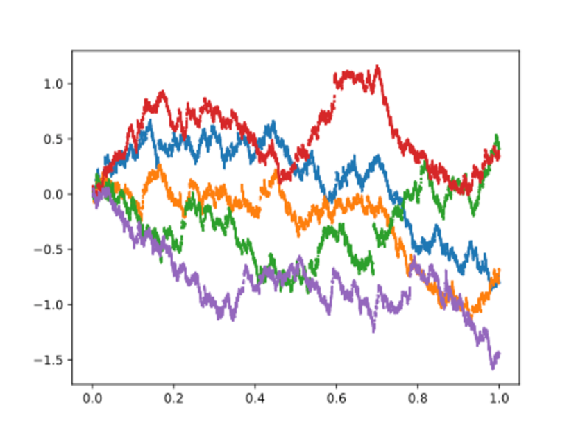
(a) $r=0.2$

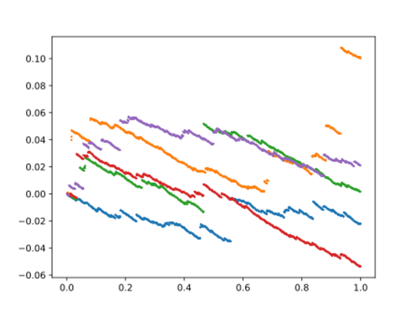
(b) $r=0.8$

Figure 1: Trajectories of $L^{m}$ when the subjacent random variable $X\sim|G|^{-r}$, where $G\sim\mathcal{N}(0,1)$. In the left column $r=0.2$, therefore the limit of $L^{m}$ is a Brownian motion and the trajectories of $L^{m}$ seem to be continuous. In the right column, $r=0.8$, hence the limit of $L^{m}$ is a Lévy process and the trajectories of $L^{m}$ seem to have jumps.

Remark 2.5.

The conclusion of Theorem 2.4 still holds true in some cases when the $X_{i}$’s are weakly dependent. Sufficient conditions to respectively obtain Brownian or stable Lévy limits can be found in Shao [14] or Tyran-Kamińska [17].

The following lemma will allow us to reformulate Theorem 2.4 as a statement where $\mu_{m}$ does not need to be known.

Lemma 2.6.

Denote by $D[0,1]$ the space of cadlag functions defined on $[0,1]$ and consider the mapping $\Psi:D[0,1]\to D[0,1]$ defined as

$$\Psi(x)(t):=x(t)-tx(1).$$

The mapping $\Psi$ is continuous for the the $J_{1}$-Skorokhod topology.

Proof.

The addition is continuous in the $J_{1}$-Skorokhod topology if one of the summands is continuous. (See e.g. Jacod and Shiryaev [10, Prop.1.23,Sec.1b,Chap.VI]). ∎

From the previous lemma and the Mapping Theorem we deduce:

Proposition 2.7.

Let

$$Z^{m}:=\left(\frac{S_{\lfloor mt\rfloor}-tS_{m}}{c_{m}},t\geq 0\right).$$ (2.1)

If $X\in\operatorname{DA}(\alpha)$, then

$$Z^{m}\xrightarrow[m\to\infty]{\mathcal{D}}Z:=\Psi(L),$$

where $L$ is a standard $\alpha$-stable Lévy process for $\alpha<2$ (and therefore $\Psi(L)$ is a discontinuous process), whereas for $\alpha=2$ $L$ is a Brownian motion (and therefore $\Psi(L)$ is a Brownian bridge).

To conclude, testing for jumps the trajectories of the limit process of $Z^{m}$ defined in (2.1) should allow one to discriminate between $X\in\operatorname{DA}(2)$ and $X\in\operatorname{DA}(\alpha),~{}0<\alpha<2$. It now remains to construct an hypothesis test for the continuity of $\Psi(L)$ which does not suppose that $c_{m}$ is known.

3 A bivariation based statistic

Determining whether a stochastic process $Y$ is continuous or not from the observation of one single path at discrete times, is an important modelling issue in many fields, notably in economics and financial mathematics. It has been addressed by several authors in the last years. See for example Ait-Sahalia and Jacod [1] and the references therein.

Our situation is somehow different since we are not observing a trajectory of a given process. We rather are constructing one discrete time path by means of a normalization procedure of our (observed or simulated) data and this constructed trajectory is always discontinuous. We therefore aim to construct a statistic whose asymptotic properties will allow us to apply detection of jumps of semimartingale methods.

Following Barndorff-Nielsen and Shephard [3], for any stochastic process $(Y_{t})_{0\leq t\leq 1}$ we set $\Delta_{i}^{n}Y=Y_{i/n}-Y_{(i-1)/n}$ and consider the realized bivariation, the realized quadratic variation and the normalized realized bivariation respectively defined by

$$\widehat{{B}}(Y,n):=\sum_{i=1}^{n-1}|\Delta_{i}^{n}Y||\Delta_{i+1}^{n}Y|,\quad\widehat{{Q}}(Y,n):=\sum_{i=1}^{n}|\Delta_{i}^{n}Y|^{2},\quad\widehat{\mathscr{S}}_{n}(Y):=\frac{\widehat{{B}}(Y,n)}{\widehat{{Q}}(Y,n)}.$$ (3.1)

In [3], the authors consider processes $(Y_{t})$ of the form

$$Y_{t}=Y_{0}+\int_{0}^{t}a_{s}~{}ds+\int_{0}^{t}\sigma_{s}~{}dW_{s}+\sum_{j=1}^{N_{t}}c_{j},$$ (3.2)

where $W$ is a Brownian motion and $(N_{t})$ is a counting process. They assume that $a$ and $\sigma$ are càdlàg processes, $c_{j}$ are non-zero random variable, $\sigma$ is pathwise bounded away from zero and the joint process $(a,\sigma)$ is independent of the Brownian motion $(W_{t})$. Barndorff-Nielsen and Shephard provided a test to decide ‘$\mathcal{H}_{0}$: $(N_{t})\equiv 0$’ against ‘$\mathcal{H}_{1}$: $(N_{t})\not\equiv 0$’.

Barndorff-Nielsen and Shephard’s test is based on the statistic

$$\frac{1}{\sqrt{n}}~{}\left(\frac{\frac{2}{\pi}\widehat{{B}}(Y,n)}{\widehat{{Q}}(Y,n)}-1\right)~{}\frac{\int_{0}^{t}\sigma_{s}^{2}~{}ds}{\sqrt{\int_{0}^{t}\sigma_{s}^{4}~{}ds}}$$

or to a similar statistic depending on $\widehat{{B}}(Y,n)$, $\widehat{{Q}}(Y,n)$ and $\int_{0}^{t}\sigma_{s}^{4}~{}ds$ only.

Barndorff-Nielsen and Shephard’s analysis of the test (see [3, Thm.1]) does not apply in our context since Brownian bridges are not of the type (3.2) with $(\sigma_{s})$ satisfying the requested constraints.

The non-degeneracy of the integrands is also needed by Ait-Sahalia and Jacod (see Assumption 1-(f) in [1, p.187]). In addition, they use the p-variation of semimartingales with $p>2$ to test continuous paths against jumps. We cannot follow the same way since we test ‘Brownian bridge’ against ‘a transformed alpha-stable process’ (recall Proposition 2.7) and the semimartingale representation of a Brownian bridge implies that the p-variation is asymptotically infinite in both cases.

We therefore need to introduce a new statistic which is adapted to our specific situation.

Definition 3.1.

For any $n\in\mathbb{N}$ consider the real-valued functional $\widehat{\mathscr{S}}_{n}$ defined as follows: for $z\in D[0,1]$,

$$\widehat{\mathscr{S}}_{n}(z):=\frac{\sum_{i=1}^{n-1}{|z(i/n)-z((i-1)/n)||z((i+1)/n)-z(i/n)|}}{\sum_{i=1}^{n}{|z(i/n)-z((i-1)/n)|^{2}}}.$$ (3.3)

Let $m\in\mathbb{N}$, given an i.i.d. sample of $X:X_{1},\ldots,X_{m}$ and the corresponding process $Z^{m}$ as in (2.1) we define our statistic $\widehat{\mathscr{S}}_{n}^{m}$ as the normalized bivariation of $Z^{m}$, that is,

$$\widehat{\mathscr{S}}_{n}^{m}:=\widehat{\mathscr{S}}_{n}(Z^{m}).$$ (3.4)

The next result provides a key property of the statistic $\widehat{\mathscr{S}}_{n}^{m}$.

Proposition 3.2.

The statistic $\widehat{\mathscr{S}}_{n}^{m}$ is scale-free and satisfies

$$\widehat{\mathscr{S}}_{n}^{m}=\frac{\sum_{i=1}^{n-1}{\left|\sum_{j=\lfloor\frac{m(i-1)}{n}\rfloor+1}^{\lfloor\frac{mi}{n}\rfloor}(X_{j}-\overline{X}_{m})\right|\left|\sum_{j=\lfloor\frac{mi}{n}\rfloor+1}^{\lfloor\frac{m(i+1)}{n}\rfloor}(X_{j}-\overline{X}_{m})\right|}}{\sum_{i=1}^{n}{\left|\sum_{j=\lfloor\frac{m(i-1)}{n}\rfloor+1}^{\lfloor\frac{mi}{n}\rfloor}(X_{j}-\overline{X}_{m})\right|^{2}}}.$$

Proof.

Observe that

$$\widehat{\mathscr{S}}_{n}^{m} :=\widehat{\mathscr{S}}_{n}(Z^{m})$$

$$=\frac{\sum_{i=1}^{n-1}{|Z_{i/n}^{m}-Z_{(i-1)/n}^{m}||Z_{(i+1)/n}^{m}-Z_{i/n}^{m}|}}{\sum_{i=1}^{n}{|Z_{i/n}^{m}-Z_{(i-1)/n}^{m}|^{2}}}$$

$$=\frac{\sum_{i=1}^{n-1}{\left|\frac{S_{\lfloor\frac{mi}{n}\rfloor}-\frac{i}{n}S_{m}}{c_{m}}-\frac{S_{\lfloor\frac{m(i-1)}{n}\rfloor}-\frac{(i-1)}{n}S_{m}}{c_{m}}\right|\left|\frac{S_{\lfloor\frac{m(i+1)}{n}\rfloor}-\frac{(i+1)}{n}S_{m}}{c_{m}}-\frac{S_{\lfloor\frac{mi}{n}\rfloor}-\frac{i}{n}S_{m}}{c_{m}}\right|}}{\sum_{i=1}^{n}{\left|\frac{S_{\lfloor\frac{mi}{n}\rfloor}-\frac{i}{n}S_{m}}{c_{m}}-\frac{S_{\lfloor\frac{m(i-1)}{n}\rfloor}-\frac{i-1}{n}S_{m}}{c_{m}}\right|^{2}}}$$

$$=\frac{\sum_{i=1}^{n-1}{\left|S_{\lfloor\frac{mi}{n}\rfloor}-S_{\lfloor\frac{m(i-1)}{n}\rfloor}-\frac{1}{n}S_{m}\right|\left|S_{\lfloor\frac{m(i+1)}{n}\rfloor}-S_{\lfloor\frac{mi}{n}\rfloor}-\frac{1}{n}S_{m}\right|}}{\sum_{i=1}^{n}{\left|S_{\lfloor\frac{mi}{n}\rfloor}-S_{\lfloor\frac{m(i-1)}{n}\rfloor}-\frac{1}{n}S_{m}\right|^{2}}}$$

$$=\frac{\sum_{i=1}^{n-1}{\left|\sum_{j=\lfloor\frac{m(i-1)}{n}\rfloor+1}^{\lfloor\frac{mi}{n}\rfloor}(X_{j}-\overline{X}_{m})\right|\left|\sum_{j=\lfloor\frac{mi}{n}\rfloor+1}^{\lfloor\frac{m(i+1)}{n}\rfloor}(X_{j}-\overline{X}_{m})\right|}}{\sum_{i=1}^{n}{\left|\sum_{j=\lfloor\frac{m(i-1)}{n}\rfloor+1}^{\lfloor\frac{mi}{n}\rfloor}(X_{j}-\overline{X}_{m})\right|^{2}}},$$

which is the desired result. ∎

Remark 3.3.

Notice that computing $\widehat{\mathscr{S}}_{n}^{m}$ only needs the values of the sample. In particular, one does not need the unknown centering and normalizing factors $\mu_{m}$ and $c_{m}$ in Theorem 2.4.

4 Our hypothesis test for domains of attraction of stable laws

In this section we present our hypothesis test for $\mathbf{H_{0}}$ against $\mathbf{H_{1}}$. It is based on the following consistency property and Central Limit Theorem for the statistic $\widehat{\mathscr{S}}_{n}^{m}$.

The consistency of $\widehat{\mathscr{S}}_{n}^{m}$ is provided by the following proposition whose lenghthy proof is postponed to Section 5.

Proposition 4.1.

For any $\epsilon>0$ one has

$$\lim_{n\to\infty}\lim_{m\to\infty}\mathbb{P}\left(|\widehat{\mathscr{S}}_{n}^{m}-\kappa|\leq\epsilon\right)=1,$$ (4.1)

with

$$\kappa:=\left\{\begin{array}[]{ccl}\frac{2}{\pi}&\text{when}&X\in\operatorname{DA}(2),\\ 0&\text{when}&X\in\operatorname{DA}(\alpha),\;\alpha<2.\end{array}\right.$$

The next proposition provides a Central Limit Theorem for the statistic $\widehat{\mathscr{S}}_{n}^{m}$. We postpone its proof to Section 6.

Proposition 4.2.

If the subjacent random variable $X$ belongs to the domain of attraction of the normal law, for any bounded and continuous function $\varphi:\mathbb{R}\to\mathbb{R}$ we have

$$\lim_{n\to\infty}\lim_{m\to\infty}\mathbb{E}\left[\varphi\left(\frac{\sqrt{n}}{\sigma_{\pi}}\left(\widehat{\mathscr{S}}_{n}^{m}-\frac{2}{\pi}\right)\right)\right]=\mathbb{E}\left[\varphi(\mathcal{N})\right],$$

where $\sigma_{\pi}^{2}=1+\frac{4}{\pi}-\frac{20}{\pi^{2}}$ and $\mathcal{N}$ is a standard Gaussian random variable.

Propositions 4.1 and 4.2 allow us to propose and analyse the following hypothesis test:

Theorem 4.3.

Assume that $X$ belongs to some domain of attraction. Consider and i.i.d. sample $X_{1},\ldots,X_{m}$ of a r.v. $X$. We consider the test hypotheses

$\mathbf{H_{0}}$: $X\in\operatorname{DA}(2)$
and
$\mathbf{H_{1}}$: $\exists 0<\alpha<2,\;X\in\operatorname{DA}(\alpha)$.

Let $z_{q}$ denote the $q$-quantile of a standard normal random variable and $\sigma_{\pi}^{2}=1+\frac{4}{\pi}-\frac{20}{\pi^{2}}$. The rejection region

$$C_{n,m}:=\left\{\left|\widehat{\mathscr{S}}_{n}^{m}-\frac{2}{\pi}\right|>z_{1-q/2}{\frac{\sigma_{\pi}}{\sqrt{n}}}\right\}{=\left\{{\frac{\sqrt{n}}{\sigma_{\pi}}}~{}(\widehat{\mathscr{S}}_{n}^{m}-\frac{2}{\pi})<z_{q/2}\right\}\bigcup\left\{{\frac{\sqrt{n}}{\sigma_{\pi}}}~{}(\widehat{\mathscr{S}}_{n}^{m}-\frac{2}{\pi})>z_{1-q/2}\right\}}$$

satisfies:

1. $\limsup_{n\to\infty}\limsup_{m\to\infty}\mathbb{P}\left(C_{n,m}|\mathbf{H_{0}}\right)\leq q$.

2. $\lim_{n\to\infty}\lim_{m\to\infty}\mathbb{P}\left(C_{n,m}|\mathbf{H_{1}}\right)=1$.

Proof.

To prove the first claim, we fix $\delta>0$ and consider the function $\psi_{\delta}:\mathbb{R}\to\mathbb{R}$ given by:

$$\psi_{\delta}(x)=\left\{\begin{array}[]{ccl}1&\text{for}&x<z_{q/2},\\ 1-\frac{1}{\delta}(x-z_{q/2})&\text{for}&z_{q/2}\leq x\leq z_{q/2}+\delta,\\ 0&\text{for}&z_{q/2}+\delta<x<z_{1-q/2}-\delta,\\ \frac{1}{\delta}(x-z_{1-q/2})&\text{for}&z_{1-q/2}\leq x\leq z_{1-q/2},\\ 1&\text{for}&z_{1-q/2}<x.\\ \end{array}\right.$$

Therefore,

$$\mathbb{P}\left(C_{n,m}|\mathbf{H_{0}}\right)\leq\mathbb{E}\left(\psi_{\delta}(\widehat{\mathscr{S}}_{n}^{m})|\mathbf{H_{0}}\right).$$

In view of Proposition 4.2 we obtain

$$\limsup_{n\to\infty}\limsup_{m\to\infty}\mathbb{P}\left(C_{n,m}|\mathbf{H_{0}}\right)\leq\mathbb{E}\left[\psi_{\delta}(\mathcal{N})\right],$$

where $\mathcal{N}$ is a standard Gaussian random variable. Thanks to the dominated convergence theorem we have

$$\lim_{\delta\to 0}\mathbb{E}\left[\psi_{\delta}(\mathcal{N})\right]=\mathbb{P}\left(\mathcal{N}<z_{q/2}\right)+\mathbb{P}\left(\mathcal{N}>z_{1-q/2}\right)=q.$$

We thus can conclude that

$$\limsup_{n\to\infty}\limsup_{m\to\infty}\mathbb{P}\left(C_{n,m}|\mathbf{H_{0}}\right)\leq q.$$

As for the second claim, it suffices to use Proposition 4.1 since under $\mathbf{H_{1}}$ it holds that

$$\forall\epsilon>0,~{}~{}\lim_{n\to\infty}\lim_{m\to\infty}\mathbb{P}\left({\widehat{\mathscr{S}}_{n}^{m}}\leq\epsilon\right)=1.$$

∎

Remark 4.4.

Other tests in the literature related to ours: In [11] Jurečková and Picek develop a statistical test for the heaviness of the tail of a distribution function $F$ assuming that $F$ is absolutely continuous and strictly increasing on the set $\{x:F(x)>0\}$. In their case, for $m_{0}$ given, the null hypothesis is

$$H_{m_{0}}:\;x^{m_{0}}(1-F(x))\geq 1,\;\;\forall x>x_{0}\text{ for some }x_{0}\geq 0,$$

whereas the alternative hypothesis is

$$K_{m_{0}}:\;\limsup_{x\to\infty}x^{m_{0}}(1-F(x))<1.$$

Notice that for $m_{0}=2$ the non-rejection $H_{m_{0}}$ implies that $F$ has infinite second moment. Although this test has a very good behavior even for small samples, it is only applicable to absolutely continuous distributions whereas our test does not need such a condition, which is essential for applications to samples produced by complex simulations of random processes. Moreover, Jurečková and Picek’s test applies to I.I.D. random variables, whereas our methodology can be extended to some weak dependence cases (see Section 7.3 below). This potentially allows applications to interacting particles which propagate chaos. Finally, we refer to [12] for other nonparametric techniques in the context of heavy tailed distributions.

5 Consistency of the statistic $\widehat{\mathscr{S}}_{n}^{m}$: Proof of Prop. 4.1

The objective of this section is to establish the consistency proposition 4.1.

To prove this proposition we need two preliminary results.

5.1 Two consistency properties of $\widehat{\mathscr{S}}_{n}$

Proposition 5.1.

Recall that we have set $Z=\Psi(L)$. For any $n\in\mathbb{N}$ it holds that

$${\widehat{\mathscr{S}}_{n}^{m}}\xrightarrow[m\to\infty]{\mathcal{D}}\widehat{\mathscr{S}}_{n}(Z).$$ (5.1)

Proof.

For any positive integer $n$ recall the functional $\widehat{\mathscr{S}}_{n}:D[0,1]\to\mathbb{R}$ defined in (3.3). This functional is not continuous on $D[0,1]$ for the Skorokhod topology. Its discontinuity set is

$$J_{n}:= \{z\in D[0,1]:\exists i=1,\ldots,n-1:\Delta z(i/n)>0\}$$

$$\cup\{z\in D[0,1]:\forall i=0,\ldots,n-1:z(i/n)=z((i-1)/n)\}.$$

Therefore, as soon as $\mathbb{P}(Z\in J_{n})=0$ we can apply the Continuous Mapping Theorem to get

$$\widehat{\mathscr{S}}_{n}(Z^{m})\xrightarrow[m\to\infty]{\mathcal{D}}\widehat{\mathscr{S}}_{n}(Z).$$

On the one hand, if the subjacent random variable $X$ belongs to $\operatorname{DA}(2)$, then $Z$ is a Brownian Bridge and therefore $\mathbb{P}(Z\in J_{n})=0$.

On the other hand, if $X$ belongs to $\operatorname{DA}(\alpha)$ with $o<\alpha<2$, then the limit process $Z$ is equal to $\Psi(L)$ where $L$ is a $\alpha$-stable process. Notice that $Z$ and $L$ hav the same jumps. Since the probability of $L$ having a jump at any fixed time is zero, it follows that $\mathbb{P}\left(Z\text{ has a jump at }i/n\right)=0$. In addition, we have

$$\mathbb{P}(Z\in J_{n})\leq\sum_{i=1}^{n-1}\mathbb{P}\left(Z\text{ has a jump at }i/n\right)+\mathbb{P}\left(Z_{i/n}=0,\;i=1,\ldots,n-1\right)=0,$$

since since $Z_{0}=Z_{1}=0$, each summand in the first term of the right-hand side is zero, and the second term in the right-hand side is zero because $\operatorname{law}(Z_{t})$ is absolutely continuous with respect to the Lebesgue measure (see Bertoin [4, p.218]).

To summarize, in both cases we have $\mathbb{P}(Z\in J_{n})=0$ and (5.1) holds true. ∎

Proposition 5.2.

Let $\Psi$ be defined as in Lemma 2.6 and $\widehat{\mathscr{S}}_{n}$ be defined as in (3.1). Then,

1. If $(Y_{t})_{0\leq t\leq 1}$ is a standard Brownian motion one has

   $$\widehat{\mathscr{S}}_{n}(\Psi(Y))\xrightarrow[n\to\infty]{\text{a.s.}}\frac{2}{\pi}.$$

2. If $(Y_{t})_{0\leq t\leq 1}$ is an $\alpha$-stable process starting from $0$ one has

   $$\forall 1<\alpha\leq 2,~{}~{}\widehat{\mathscr{S}}_{n}(\Psi(Y))\xrightarrow[n\to\infty]{\text{a.s.}}0.$$

   For $\alpha\leq 1$ the convergence holds in probability only.

Proof.

In view of (3.1) we succesively consider $\widehat{{Q}}(\Psi(Y),n)$ and $\widehat{{B}}(\Psi(Y),n)$.

A straightforward computation leads to

$$\widehat{{Q}}(\Psi(Y),n)=\widehat{{Q}}(Y,n)-\frac{1}{n}Y_{1}^{2}.$$ (5.2)

The second term in the right-hand side converges to zero a.s. We thus have to prove the a.s. convergence of $\widehat{{Q}}(Y,n)$.

When $Y$ is a standard Brownian motion we have

$$\widehat{{Q}}(Y,n)=\frac{1}{n}\sum_{i=1}^{n}\left(\sqrt{n}\Delta_{i}^{n}Y\right)^{2}\xrightarrow[n\to\infty]{\text{a.s.}}1,$$

thanks to the Strong Law of Large Numbers, from which

$$\widehat{{Q}}(\Psi(Y),n)\xrightarrow[n\to\infty]{\text{a.s.}}1$$ (5.3)

and

$$\lim_{n\to\infty}\widehat{\mathscr{S}}_{n}(\Psi(Y))=\lim_{n\to\infty}\frac{\widehat{{B}}(\Psi(Y),n)}{\widehat{{Q}}(\Psi(Y),n)}=\lim_{n\to\infty}\widehat{{B}}(\Psi(Y),n).$$

Consequently, the first statement of the proposition results from the two following results which will be proven in the next subsection (see Lemmas 5.3 and 5.4): For any Brownian motion $Y$,

$$\widehat{{B}}(Y,n)\xrightarrow[n\to\infty]{\text{a.s.}}\frac{2}{\pi}$$

and

$$\widehat{{B}}(Y,n)-\widehat{{B}}(\Psi(Y),n)\xrightarrow[n\to\infty]{\text{a.s.}}0.$$

Now, when $Y$ is an $\alpha$-stable process with $\alpha<2$ we have

$$\widehat{{Q}}(Y,n)=\sum_{i=1}^{n}\left(\Delta_{i}^{n}Y\right)^{2}=\frac{1}{n^{2/\alpha}}\sum_{i=1}^{n}\left(n^{1/\alpha}\Delta_{i}^{n}Y\right)^{2}$$

and the positive random variable $U_{i}=\left(n^{1/\alpha}\Delta_{i}^{n}Y\right)^{2}$ satisfies $\mathbb{P}(U_{i}>t)\sim t^{-\alpha/2}$. Consequently, as $n$ goes to infinity, $\widehat{{Q}}(Y,n)$ converges in distribution to a stable law $Q$ with index $\frac{\alpha}{2}<1$, from which $\mathbb{P}(Q=0)=0$. From (5.2) it follows that $\widehat{{Q}}(\Psi(Y),n)$ also converges in distribution to $Q$. We now use the two following results which will be proven in the next subsection: If $Y$ is an $\alpha$-stable process starting from 0, then

$$\widehat{{B}}(Y,n)\xrightarrow[n\to\infty]{\text{a.s.}}0$$

and

$$\lim_{n\to\infty}\widehat{{B}}(\Psi(Y),n)=\lim_{n\to\infty}\widehat{{B}}(Y,n),$$

where the limit is in probability.

Consequently, in view of Slutsky’s lemma,

$$\widehat{\mathscr{S}}_{n}(\Psi(Y))=\frac{\widehat{{B}}(\Psi(Y),n)}{\widehat{{Q}}(\Psi(Y),n)}\xrightarrow[n\to\infty]{\mathbb{P}}0.$$

∎

In the proof of Proposition 5.2 we have used the two following lemmas.

5.2 Two key lemmas

The first point of the first Lemma in this subsection is contained in Barndorff-Nielsen and Shephard [3, Thm.4.]. We here give its easy proof for the sake of completeness. The second point requires less obvious arguments.

Lemma 5.3.

We have:

1. Let $(Y_{t})_{0\leq t\leq 1}$ be a standard Brownian motion, then

   $$\widehat{{B}}(Y,n)\xrightarrow[n\to\infty]{\text{a.s.}}\frac{2}{\pi}.$$

2. Let $(Y_{t})_{0\leq t\leq 1}$ be an $\alpha$-stable process starting from $0$. For $\alpha>1$, we have

   $$\widehat{{B}}(Y,n)\xrightarrow[n\to\infty]{\text{a.s.}}0,$$

   whereas for $\alpha\leq 1$ this last convergence holds in probability only.

Proof.

1. Let $(Y_{t})_{0\leq t\leq 1}$ be a Brownian motion. Then,

   $$\sum_{i=1}^{n-1}|\Delta_{i}^{n}Y||\Delta_{i+1}^{n}Y| =\sum_{i=1}^{\lfloor n/2\rfloor}|\Delta_{2i-1}Y||\Delta_{2i}Y|+\sum_{i=1}^{\lfloor n/2\rfloor-1}|\Delta_{2i}Y||\Delta_{2i+1}Y|$$

   $$\quad+2\left(\frac{n}{2}-\lfloor\frac{n}{2}\rfloor\right)|\Delta_{n-1}^{n}Y||\Delta_{n}^{n}Y|$$

   $$=\frac{1}{2}\frac{2}{n}\sum_{i=1}^{\lfloor n/2\rfloor}|\sqrt{n}\Delta_{2i-1}Y||\sqrt{n}\Delta_{2i}Y|+\frac{1}{2}\frac{2}{n}\sum_{i=1}^{\lfloor n/2\rfloor-1}|\sqrt{n}\Delta_{2i}Y||\sqrt{n}\Delta_{2i+1}Y|$$

   $$\quad+2\left(\frac{n}{2}-\lfloor\frac{n}{2}\rfloor\right)|\Delta_{n-1}^{n}Y||\Delta_{n}^{n}Y|.$$

   Notice that $\sqrt{n}\Delta_{i}Y\sim\mathcal{N}(0,1)$. The Law of the Large Numbers imples

   $$\frac{2}{n}\sum_{i=1}^{\lfloor n/2\rfloor}|\sqrt{n}\Delta_{2i-1}Y||\sqrt{n}\Delta_{2i}Y|\xrightarrow[n\to\infty]{\text{a.s.}}\frac{2}{\pi},$$

   $$\frac{2}{n}\sum_{i=1}^{\lfloor n/2\rfloor}|\sqrt{n}\Delta_{2i}Y||\sqrt{n}\Delta_{2i+1}Y|\xrightarrow[n\to\infty]{\text{a.s.}}\frac{2}{\pi}.$$

   In addition, the continuity of the trajectories of the Brownian motion implies that

   $$\left|2\left(\frac{n}{2}-\lfloor\frac{n}{2}\rfloor\right)|\Delta_{n-1}^{n}Y||\Delta_{n}^{n}Y|\right|\leq 2|\Delta_{n-1}^{n}Y||\Delta_{n}^{n}Y|\xrightarrow[n\to\infty]{\text{a.s.}}0,$$

   Putting all together we get

   $$\widehat{{B}}(Y,n)\xrightarrow[n\to\infty]{\text{a.s.}}\frac{2}{\pi}.$$

2. Let $(Y_{t})_{0\leq t\leq 1}$ be an $\alpha$-stable process starting from $0$. In this case we have

   $$\widehat{{B}}(Y,n) =\frac{1}{2}\frac{2}{n^{2/\alpha}}\sum_{i=1}^{\lfloor n/2\rfloor}|n^{1/\alpha}\Delta_{2i-1}Y||n^{1/\alpha}\Delta_{2i}Y|+\frac{1}{2}\frac{2}{n^{2/\alpha}}\sum_{i=1}^{\lfloor n/2\rfloor-1}|n^{1/\alpha}\Delta_{2i}Y||n^{1/\alpha}\Delta_{2i+1}Y|$$

   $$\quad+2\left(\frac{n}{2}-\lfloor\frac{n}{2}\rfloor\right)|\Delta_{n-1}^{n}Y||\Delta_{n}^{n}Y|,$$

   and for any $i=1,\ldots,n$, $n^{1/\alpha}\Delta_{i}Y$ are independent $\alpha$-stable random variables. We proceed by cases:

   • $\alpha\in(1,2):$ Notice that

     $$\frac{2}{n^{2/\alpha}}\sum_{i=1}^{\lfloor n/2\rfloor}|n^{1/\alpha}\Delta_{2i-1}Y||n^{1/\alpha}\Delta_{2i}Y|=\frac{1}{n^{2/\alpha-1}}\left(\frac{2}{n}\sum_{i=1}^{\lfloor n/2\rfloor}|n^{1/\alpha}\Delta_{2i-1}Y||n^{1/\alpha}\Delta_{2i}Y|\right).$$

     The Law of Large Numbers implies that the term inside the parenthesis in the right-hand side a.s. converges to a finite quantity. Therefore the whole right-hand side a.s. tends to 0. Similarly,

     $$\frac{2}{n^{2/\alpha}}\sum_{i=1}^{\lfloor n/2\rfloor-1}|n^{1/\alpha}\Delta_{2i}Y||n^{1/\alpha}\Delta_{2i+1}Y|\xrightarrow[n\to\infty]{\text{a.s.}}0.$$

     We finally observe that

     $$\limsup_{n\to\infty}\left|2\left(\frac{n}{2}-\lfloor\frac{n}{2}\rfloor\right)|\Delta_{n-1}^{n}Y||\Delta_{n}^{n}Y|\right|\leq 2\lim_{n\to\infty}\left|Y_{1}-Y_{1-\frac{1}{n}}\right|\left|Y_{1-\frac{1}{n}}-Y_{1-\frac{2}{n}}\right|=0\;\;\text{a.s.}$$

     since the paths of $Y$ have left limits. Therefore, for $\alpha\in(1,2)$ we have

     $$\widehat{{B}}(Y,n)\xrightarrow[n\to\infty]{\text{a.s.}}0.$$

   • $\alpha\in(0,1):$ In view of Embrechts and Goldie [5, Cor. of Thm.3] we have that $|n^{1/\alpha}\Delta_{2i-1}Y||n^{1/\alpha}\Delta_{2i}Y|\in\operatorname{DA}(\alpha)$. Therefore, there exists a slowly varying function $\ell_{0}$ such that

     $$\frac{1}{n^{1/\alpha}\ell_{0}(n)}\sum_{i=1}^{\lfloor n/2\rfloor}|n^{1/\alpha}\Delta_{2i-1}Y||n^{1/\alpha}\Delta_{2i}Y|,$$

     converges in distribution to an $\alpha$-stable random variable. Hence

     $$\frac{2}{n^{2/\alpha}}\sum_{i=1}^{\lfloor n/2\rfloor}|n^{1/\alpha}\Delta_{2i-1}Y||n^{1/\alpha}\Delta_{2i}Y|=\frac{\ell_{0}(n)}{n^{1/\alpha}}\frac{1}{n^{1/\alpha}\ell_{0}(n)}\sum_{i=1}^{\lfloor n/2\rfloor}|n^{1/\alpha}\Delta_{2i-1}Y||n^{1/\alpha}\Delta_{2i}Y|$$

     tends to zero in probability, because is the product of a sequence of random variables converging in distribution and a real sequence converging to zero. For the other terms we can proceed as before. We thus are in a position to conclude that

     $$\widehat{{B}}(Y,n)\xrightarrow[n\to\infty]{\mathbb{P}}0.$$

   • $\alpha=1:$ We need to study normalized sums of the type

     $$\frac{1}{2}\frac{2}{n^{2}}\sum_{i=1}^{\lfloor n/2\rfloor}|n\Delta_{2i-1}Y||n\Delta_{2i}Y|.$$

     Denote by $A$ such a quantity. Notice that for each $i$, $n\Delta_{i}Y$ has a $1$-stable law. By again using Embrechts and Goldie [5, Cor. of Thm.3] we get that $|n\Delta_{2i-1}Y|n\Delta_{2i}Y|$ belongs to $\operatorname{DA}(1)$. Hence, we need to introduce centering factors to obtain the convergence of $A$.

     In view of Whitt [18, Thm.4.5.1] the centered and normalized sums

     $$\frac{1}{(n/2)\ell_{0}(n/2)} \Bigg{(}\sum_{i=1}^{\lfloor n/2\rfloor}|n\Delta_{2i-1}Y||n\Delta_{2i}Y|$$

     $$\quad-(n/2)^{2}\ell_{0}(n/2)\mathbb{E}\left[\sin\left(\frac{|n\Delta_{2i-1}Y||n\Delta_{2i}Y|}{(n/2)\ell_{0}(n/2)}\right)\right]\Bigg{)}$$

     converge in distribution to a $1$-stable random variable. Then

     $$A =\frac{\ell_{0}(n/2)}{2n}\Big{(}\text{Converging in Distribution Sequence}\Big{)}$$

     $$\quad+\ell_{0}(n/2)\mathbb{E}\left[\sin\left(\frac{|n\Delta_{1}Y||n\Delta_{2}Y|}{(n/2)\ell_{0}(n/2)}\right)\right],$$

     The first term tends to $0$ in probability because is the product of a deterministic sequence converging to $0$ and a weakly convergent sequence of random variables. As for the second one, there exist $1$-stable random variables $S_{1}$ and $S_{2}$ such that

     $$\ell_{0}(n/2)\mathbb{E}\left[\sin\left(\frac{|n\Delta_{2i-1}Y||n\Delta_{2i}Y|}{(n/2)\ell_{0}(n/2)}\right)\right] =\ell_{0}(n/2)\mathbb{E}\left[\sin\left(\frac{|S_{1}S_{2}|}{(n/2)\ell_{0}(n/2)}\right)\right]$$

     $$\leq\mathbb{E}\left[\sqrt{|S_{1}|}\right]^{2}\frac{\sqrt{\ell_{0}(n/2)}}{\sqrt{n/2}},$$

     where in the last inequality we have used $|\sin(x)|\leq\sqrt{|x|}$. Hence the right-hand side converges to $0$. We thus conclude that

     $$\widehat{{B}}(Y,n)\xrightarrow[n\to\infty]{\mathbb{P}}0.$$

∎

The second lemma in this subsection shows that $\widehat{{B}}(Y,n)$ and $\widehat{{B}}(\Psi(Y),n)$ have a similar asymptotic behaviour.

Lemma 5.4.

If $(Y_{t})_{0\leq t\leq 1}$ is, either a Brownian motion or an $\alpha$-stable process starting from $0$ with $\alpha>1$, then

$$\widehat{{B}}(Y,n)-\widehat{{B}}(\Psi(Y),n)\xrightarrow[n\to\infty]{\text{a.s.}}0.$$

Moreover, if $(Y_{t})_{0\leq t\leq 1}$ is an $\alpha$-stable process starting from $0$ with $\alpha\leq 1$ this last convergence holds in probability only.

Proof of Lemma 5.4 .

Since for all $a,b\in\mathbb{R}$ $||a|-|b||\leq|a-b|$, we have

$$\left|\sum_{i=1}^{n-1}|\Delta_{i}^{n}\Psi(Y)||\Delta_{i+1}^{n}\Psi(Y)|-\sum_{i=1}^{n-1}|\Delta_{i}^{n}Y||\Delta_{i+1}^{n}Y|\right| \leq\sum_{i=1}^{n-1}\left|\Delta_{i}^{n}\Psi(Y)\Delta_{i+1}^{n}\Psi(Y)-\Delta_{i}^{n}Y\Delta_{i+1}^{n}Y\right|,$$

and then

$$\left|\sum_{i=1}^{n-1}|\Delta_{i}^{n}\Psi(Y)||\Delta_{i+1}^{n}\Psi(Y)|-\sum_{i=1}^{n-1}|\Delta_{i}^{n}Y||\Delta_{i+1}^{n}Y|\right| \leq\sum_{i=1}^{n-1}\left|\frac{Y_{1}}{n}\Delta_{i}^{n}Y\right|+\sum_{i=1}^{n-1}\left|\frac{Y_{1}}{n}\Delta_{i+1}^{n}Y\right|$$ (5.4)

$$\quad+\sum_{i=1}^{n-1}\left|\frac{1}{n^{2}}Y_{1}^{2}\right|.$$

We now analyze each term in the right-hand side of (5.4). We start with the third one:

$$\sum_{i=1}^{n-1}\left|\frac{1}{n^{2}}Y_{1}^{2}\right|=\frac{(n-1)}{n^{2}}Y_{1}^{2}\xrightarrow[n\to\infty]{\text{a.s.}}0.$$

As for the second term in the right-hand side of (5.4), we have

$$\sum_{i=1}^{n-1}\left|\frac{Y_{1}}{n}\Delta_{i}^{n}Y\right|=\frac{|Y_{1}|}{n^{1/\alpha}}\frac{1}{n}\sum_{i=1}^{n-1}\left|n^{1/\alpha}\Delta_{i}^{n}Y\right|.$$

Notice that, for $i=1,\ldots,n-1$, $|n^{1/\alpha}\Delta_{i}^{n}Y|$ are i.i.d. random variables with stable law of index $\alpha$.

When $Y$ is a Brownian motion or when $\alpha>1$, there exists $y\in\mathbb{R}$ such that $\mathbb{E}\left[|n^{1/\alpha}\Delta_{i}^{n}Y|\right]=y$ for any $n\geq 1$. Then, the Law of Large Numbers implies

$$\frac{1}{n}\sum_{i=1}^{n-1}\left|n^{1/\alpha}\Delta_{i}^{n}Y\right|\xrightarrow[n\to\infty]{\text{a.s.}}y,$$

from which

$$\sum_{i=1}^{n-1}\left|\frac{Y_{1}}{n}\Delta_{i}^{n}Y\right|=\frac{|Y_{1}|}{n^{1/\alpha}}\frac{1}{n}\sum_{i=1}^{n-1}\left|n^{1/\alpha}\Delta_{i}^{n}Y\right|\xrightarrow[n\to\infty]{\text{a.s.}}0.$$

When $\alpha<1$ we use Embrechts et al. [6, Thm.2.2.15] to get that there exists a slowly varying function $\ell_{0}$ such that

$$\frac{1}{\ell_{0}(n)}\sum_{i=1}^{n-1}\left|\Delta_{i}^{n}Y\right|$$

converges in distribution as $n\to\infty$ to a stable random variable. Therefore,

$$\sum_{i=1}^{n-1}\left|\frac{Y_{1}}{n}\Delta_{i}^{n}Y\right| =\frac{|Y_{1}\ell_{0}(n)|}{n}\frac{1}{\ell_{0}(n)}\sum_{i=1}^{n-1}\left|\Delta_{i}^{n}Y\right|,$$

is the product of a random variable which a.s. converges to 0 when $n$ goes to infinity and of a random variable which converges in distribution, and thus converges to 0 in probability.

Finally, if $\alpha=1$, we have that $n\Delta_{i}^{n}Y\in\operatorname{DA}(1)$. Therefore, in view of Whitt [18, Thm.4.5.1], there exists a slowly varying function $\ell_{0}$ such that

$$\frac{1}{n\ell_{0}(n)}\left(\sum_{i=1}^{n}|n\Delta_{i}^{n}Y|-n^{2}\ell_{0}(n)\mathbb{E}\left[\sin\left(\frac{n\Delta_{1}^{n}Y}{n\ell_{0}(n)}\right)\right]\right)$$

converges in distribution to a stable distribution. We conclude that

$$\sum_{i=1}^{n-1}\left|\frac{Y_{1}}{n}\Delta_{i}^{n}Y\right| =\frac{\ell_{0}(n)|Y_{1}|}{n}\frac{1}{n\ell_{0}(n)}\left(\sum_{i=1}^{n}|n\Delta_{i}^{n}Y|-n^{2}\ell_{0}(n)\mathbb{E}\left[\sin\left(\frac{n\Delta_{1}^{n}Y}{n\ell_{0}(n)}\right)\right]\right)$$

$$\quad+\ell_{0}(n)\mathbb{E}\left[\sin\left(\frac{n\Delta_{1}^{n}Y}{n\ell_{0}(n)}\right)\right]$$

converges to zero in probability since the first term in the right-hand side is the product of a random variable which converges to zero a.s. when $n$ goes to infinity and a a random variables whcih converges in distribution. As for the second term in the right-hand side, one can check that it goes to zero by proceeding as in the end of the proof of the previous proposition. To summarize, we have

$$\sum_{i=1}^{n-1}\left|\frac{Y_{1}}{n}\Delta_{i}^{n}Y\right|\xrightarrow[n\to\infty]{\mathbb{P}}0.$$

We thus have obtained that

$$\sum_{i=1}^{n-1}\left|\frac{Y_{1}}{n}\Delta_{i+1}^{n}Y\right|\xrightarrow[n\to\infty]{\mathbb{P}}0$$

and

$$\left|\sum_{i=1}^{n-1}|\Delta_{i}^{n}\Psi(Y)||\Delta_{i+1}^{n}\Psi(Y)|-\sum_{i=1}^{n-1}|\Delta_{i}^{n}Y|~{}|\Delta_{i+1}^{n}Y|\right|\xrightarrow[n\to\infty]{\mathbb{P}}0.$$

∎

5.3 End of the proof of Proposition 4.1

We now are in a position to prove the proposition 4.1.

We start with proving that for any bounded and continuous function  $\varphi:\mathbb{R}\to\mathbb{R}$ we have

$$\lim_{n\to\infty}\lim_{m\to\infty}\mathbb{E}\left[\varphi({\widehat{\mathscr{S}}_{n}^{m}})\right]=\varphi(\kappa).$$ (5.5)

In view of Proposition 5.1 we have:

$$\lim_{m\to\infty}\left|\mathbb{E}\left[\varphi({\widehat{\mathscr{S}}_{n}^{m}})\right]-\mathbb{E}\left[\varphi(\widehat{\mathscr{S}}_{n}(Z))\right]\right|=0.$$

In addition, in view of Proposition 5.2 we have

$$\lim_{n\to\infty}\left|\mathbb{E}\left[\varphi(\widehat{\mathscr{S}}_{n}(Z))\right]-\varphi(\kappa)\right|=0.$$

Therefore, the desired limit in (5.5) is obtained by letting $m$ and then $n$ tend to infinity in the right-hand side of

$$\left|\mathbb{E}\left[\varphi({\widehat{\mathscr{S}}_{n}^{m}})\right]-\varphi(\kappa)\right|\leq\left|\mathbb{E}\left[\varphi({\widehat{\mathscr{S}}_{n}^{m}})\right]-\mathbb{E}\left[\varphi(\widehat{\mathscr{S}}_{n}(Z))\right]\right|+\left|\mathbb{E}\left[\varphi(\widehat{\mathscr{S}}_{n}(Z))\right]-\varphi(\kappa)\right|.$$

Now, fix $\epsilon>0$ and define the function $\psi$ as follows: $\psi$ takes the value $0$ outside the closed interval $[\kappa-\epsilon,\kappa+\epsilon]$, growths linearly from 0 to 1 on $[\kappa-\epsilon,\kappa]$ and decreases linearly from 1 to 0 on $[\kappa,\kappa+\epsilon]$. From

$$\mathbb{P}\left(|\widehat{\mathscr{S}}_{n}^{m}-\kappa|\leq\epsilon\right)=\mathbb{E}\left[\mathds{1}_{[\kappa-\epsilon,\kappa+\epsilon]}(\widehat{\mathscr{S}}_{n}^{m})\right]\geq\mathbb{E}\left[\varphi(\widehat{\mathscr{S}}_{n}^{m})\right],$$

it results that

$$\lim_{n\to\infty}\lim_{m\to\infty}\mathbb{P}\left(|\widehat{\mathscr{S}}_{n}^{m}-\kappa|\leq\epsilon\right)]\geq\lim_{n\to\infty}\lim_{m\to\infty}\mathbb{E}\left[\varphi(\widehat{\mathscr{S}}_{n}^{m})\right]=\varphi(\kappa)=1.$$

6 A CLT for $\widehat{\mathscr{S}}_{n}^{m}$: Proof of Prop. 4.2

In this section we prove a Central Limit theorem for $\widehat{\mathscr{S}}_{n}^{m}$ defined as in Proposition 4.2.

We start with proving the CLT for the pair $(\widehat{{B}}(Y,n),\widehat{{Q}}(Y,n))$, with $(Y_{t})_{0\leq t\leq 1}$ being a Brownian Motion.

6.1 Three CLT for $(\widehat{{B}}(Y,n),\widehat{{Q}}(Y,n))$

The first result in this subsection concerns the case where $Y$ is a Brownian motion. It is a particular case of Barndorff-Nielsen and Shephard [3, Thm.3]. For the sake of completeness we here provide a straightforward proof adapted to the specific Brownian case.

Lemma 6.1.

Let $(Y_{t})_{0\leq t\leq 1}$be a Brownian motion. One then has

$$\left(\sqrt{n}\left[\widehat{{B}}(Y,n)-\frac{2}{\pi}\right],\sqrt{n}\left[\widehat{{Q}}(Y,n)-1\right]\right)\xrightarrow[n\to\infty]{\mathcal{D}}\mathcal{N}_{2}\left(0,\Sigma\right),$$

where

$$\Sigma=\left(\begin{array}[]{cc}1+\frac{4}{\pi}-\frac{12}{\pi^{2}}&\frac{4}{\pi}\\ \frac{4}{\pi}&2\end{array}\right).$$ (6.1)

Proof.

Notice that

$$\Bigg{(}\sqrt{n} \left[\widehat{{B}}(Y,n)-\frac{2}{\pi}\right],\sqrt{n}\left[\widehat{{Q}}(Y,n)-1\right]\Bigg{)}$$

$$=\frac{1}{\sqrt{n}}\Bigg{(}\sum_{i=1}^{n-1}|\sqrt{n}\Delta_{i}^{n}Y||\sqrt{n}\Delta_{i+1}^{n}Y|-\frac{2}{\pi},\sum_{i=1}^{n-}|\sqrt{n}\Delta_{i}^{n}Y|^{2}-1\Bigg{)}.$$

The right-hand side has the same law as

$$\frac{1}{\sqrt{n}}\left(\sum_{i=1}^{n-1}\left[|G_{i}||G_{i+1}|-\frac{2}{\pi}\right],\sum_{i=1}^{n}\left[G_{i}^{2}-1\right]\right),$$

where $G_{i}$ is a standard Normal random variable.

The vectors $(|G_{i}||G_{i+1}|-{2}/{\pi},G_{i}^{2}-1)$ are identically distributed, centered, and such that $(|G_{i}||G_{i+1}|-{2}/{\pi},G_{i}^{2}-1)$ is independent of $(|G_{j}||G_{j+1}|-{2}/{\pi},G_{j}^{2}-1)$ if $|j-i|>1$. Hence, we can apply the Central Limit Theorem for $1$-dependent sequences of vectors (see Hoeffding and Robbins [9, Thm.3]). The asymptotic covariance matrix is given by

$$\Sigma_{11}:=\mathbb{E}\left[\left(|G_{i+1}||G_{i+2}|-\frac{2}{\pi}\right)^{2}\right]+2\mathbb{E}\left[\left(|G_{i}||G_{i+1}|-\frac{2}{\pi}\right)\left(|G_{i+1}||G_{i+2}|-\frac{2}{\pi}\right)\right]=1+\frac{4}{\pi}-\frac{12}{\pi^{2}},$$

$$\Sigma_{12}:=\mathbb{E}\left[\left(|G_{1}||G_{2}|-\frac{2}{\pi}\right)\left(G_{1}^{2}-1\right)\right]+\mathbb{E}\left[\left(|G_{1}||G_{2}|-\frac{2}{\pi}\right)\left(G_{2}^{2}-1\right)\right]+\mathbb{E}\left[\left(|G_{2}||G_{3}|-\frac{2}{\pi}\right)\left(G_{1}^{2}-1\right)\right]=\frac{4}{\pi},$$

and

$$\Sigma_{22}:=\mathbb{E}\left[\left(G_{1}^{2}-1\right)^{2}\right]+2\mathbb{E}\left[\left(G_{1}^{2}-1\right)\left(G_{2}^{2}-1\right)\right]=2.$$

∎

In the next Lemma we extend the previous result to Brownian Bridges.

Lemma 6.2.

Let $(Y_{t})_{0\leq t\leq 1}$ be a Brownian motion. Then

$$\mathbb{E}\left[\left(\sqrt{n}\left[\widehat{{B}}(\Psi(Y),n)-\widehat{{B}}(Y,n)\right]\right)^{2}\right]+\mathbb{E}\left[\left(\sqrt{n}\left[\widehat{{Q}}(\Psi(Y),n)-\widehat{{Q}}(Y,n)\right]\right)^{2}\right]\leq\frac{C}{n}.$$ (6.2)

In addition, one has

$$\left(\sqrt{n}\left[\widehat{{B}}(\Psi(Y),n)-\frac{2}{\pi}\right],\sqrt{n}\left[\widehat{{Q}}(\Psi(Y),n)-1\right]\right)\xrightarrow[n\to\infty]{\mathcal{D}}\mathcal{N}_{2}\left(0,\Sigma\right),$$ (6.3)

where $\Sigma$ is defined as in (6.1).

Proof.

A straightforward computation shows that

$$\widehat{{Q}}(\Psi(Y),n)=\widehat{{Q}}(Y,n)-\frac{1}{n}Y_{1}^{2}.$$

Therefore, we have

$$\mathbb{E}\left[\left(\sqrt{n}\left[\widehat{{Q}}(\Psi(Y),n)-\widehat{{Q}}(Y,n)\right]\right)^{2}\right]=\mathbb{E}\left[\frac{1}{n}Y_{1}^{4}\right]=\frac{3}{n}.$$

Now consider a family of independent random variables $G_{i}\sim\mathcal{N}(0,1)$ and set $\bar{G}^{n}:=n^{-1}\sum_{i=1}^{n}G_{i}$. It holds that

$$\mathbb{E}\left[\left(\sqrt{n}\left[\widehat{{B}}(\Psi(Y),n)-\widehat{{B}}(Y,n)\right]\right)^{2}\right] =n\sum_{i=1}^{n-1}\sum_{k=1}^{n-1}\mathbb{E}\bigg{[}\left(|\Delta_{i}^{n}\Psi(Y)||\Delta_{i+1}^{n}\Psi(Y)|-|\Delta_{i}^{n}Y||\Delta_{i+1}^{n}Y|\right)$$

$$\qquad\qquad\times\left(|\Delta_{k}^{n}\Psi(Y)||\Delta_{k+1}^{n}\Psi(Y)|-|\Delta_{k}^{n}Y||\Delta_{k+1}^{n}Y|\right)\bigg{]}$$

$$=\frac{1}{n}\sum_{i=1}^{n-1}\sum_{k=1}^{n-1}\mathbb{E}\bigg{[}\left(|G_{i}-\bar{G}^{n}||G_{i+1}-\bar{G}^{n}|-|G_{i}||G_{i+1}|\right)$$

$$\qquad\qquad\times\left(|G_{k}-\bar{G}^{n}||G_{k+1}-\bar{G}^{n}|-|G_{k}||G_{k+1}|\right)\bigg{]}$$

$$=:S_{1}+S_{2},$$

where we have split the sum according to $k=i,i+1$ in $S_{1}$ and $k\notin\{i,i+1\}$ in $S_{2}$.

As for $S_{1}$, notice that

$$|G_{i}-\bar{G}^{n}||G_{i+1}-\bar{G}^{n}|-|G_{i}||G_{i+1}|\leq|\bar{G}^{n}||\bar{G}^{n}-G_{i}-G_{i+1}|,$$

and therefore

$$S_{1} =\frac{1}{n}\sum_{i=1}^{n-2}\sum_{k=i}^{i+1}\mathbb{E}\left[\left(|G_{i}-\bar{G}^{n}||G_{i+1}-\bar{G}^{n}|-|G_{i}||G_{i+1}|\right)\left(|G_{k}-\bar{G}^{n}||G_{k+1}-\bar{G}^{n}|-|G_{k}||G_{k+1}|\right)\right]$$

$$\leq\frac{1}{n}\sum_{i=1}^{n-2}\sum_{k=i}^{i+1}\sqrt{\mathbb{E}\left[\left(|G_{i}-\bar{G}^{n}||G_{i+1}-\bar{G}^{n}|-|G_{i}||G_{i+1}|\right)^{2}\right]}$$

$$\quad\quad\times\sqrt{\mathbb{E}\left[\left(|G_{k}-\bar{G}^{n}||G_{k+1}-\bar{G}^{n}|-|G_{k}||G_{k+1}|\right)^{2}\right]}$$

$$\leq\frac{1}{n}\sum_{i=1}^{n-2}\sum_{k=i}^{i+1}\sqrt{\mathbb{E}\left[|\bar{G}^{n}|^{2}|\bar{G}^{n}-G_{i}-G_{i+1}|^{2}\right]\mathbb{E}\left[|\bar{G}^{n}|^{2}|\bar{G}^{n}-G_{k}-G_{k+1}|^{2}\right]}$$

$$\leq\frac{1}{n}\sum_{i=1}^{n-2}\sum_{k=i}^{i+1}\sqrt[4]{\mathbb{E}\left[|\bar{G}^{n}|^{4}\right]\mathbb{E}\left[|\bar{G}^{n}-G_{i}-G_{i+1}|^{4}\right]\mathbb{E}\left[|\bar{G}^{n}|^{4}\right]\mathbb{E}\left[|\bar{G}^{n}-G_{k}-G_{k+1}|^{4}\right]}$$

$$\leq\frac{C}{n}.$$

As for $S_{2}$, we use the following inequality which we admit for a while (see Subsection 6.4 for its proof):

$$\mathbb{E}\bigg{[}\left(|G_{i}-\bar{G}^{n}||G_{i+1}-\bar{G}^{n}|-|G_{i}||G_{i+1}|\right)\left(|G_{k}-\bar{G}^{n}||G_{k+1}-\bar{G}^{n}|-|G_{k}||G_{k+1}|\right)\bigg{]}\leq\frac{C}{n^{2}}.$$ (6.4)

This ends the proof of (6.2).

From  (6.2) it follows that $(\sqrt{n}[\widehat{{B}}(\Psi(Y),n)-\widehat{{B}}(Y,n)],\sqrt{n}[\widehat{{Q}}(\Psi(Y),n))-\widehat{{Q}}(Y,n))]$ converges in probability to zero. Therefore, Slutsky’s Theorem implies that

$$\left(\sqrt{n}\left[\widehat{{B}}(\Psi(Y),n)-\frac{2}{\pi}\right]\right. ,\left.\sqrt{n}\left[\widehat{{Q}}(\Psi(Y),n)-1\right]\right)$$

$$=\left(\sqrt{n}\left[\widehat{{B}}(\Psi(Y),n)-\widehat{{B}}(Y,n)\right],\sqrt{n}\left[\widehat{{Q}}(\Psi(Y),n))-\widehat{{Q}}(Y,n))\right]\right)$$

$$\quad+\left(\sqrt{n}\left[\widehat{{B}}(Y,n)-\frac{2}{\pi}\right],\sqrt{n}\left[\widehat{{Q}}(Y,n)-1\right]\right)$$

converges in distribution to $\mathcal{N}_{2}(0,\Sigma)$.

∎

We thus now in a position to obtain the following result.

Proposition 6.3.

Let $(Y_{t})_{0\leq t\leq 1}$ be a Brownian motion. One then has:

$$\sqrt{n}\left[\widehat{\mathscr{S}}_{n}(\Psi(Y))-\frac{2}{\pi}\right]\xrightarrow[n\to\infty]{\mathcal{D}}\mathcal{N}\left(0,1+\frac{4}{\pi}-\frac{20}{\pi^{2}}\right).$$

Proof.

Notice that

$$\sqrt{n}\left[\frac{\widehat{{B}}(\Psi(Y),n)}{\widehat{{Q}}(\Psi(Y),n)}-\frac{2}{\pi}\right] =\frac{\sqrt{n}}{\widehat{{Q}}(\Psi(Y),n)}\left[\widehat{{B}}(\Psi(Y),n)-\frac{2}{\pi}\widehat{{Q}}(\Psi(Y),n)\right]$$

$$=\frac{1}{\widehat{{Q}}(\Psi(Y),n)}\left(\sqrt{n}\left[\widehat{{B}}(\Psi(Y),n)-\frac{2}{\pi}\right]-\frac{2}{\pi}\sqrt{n}\left[\widehat{{Q}}(\Psi(Y),n)-1\right]\right).$$

In view of Lemma 6.2 the term in the parenthesis in the right-hand side converges to a centered Gaussian random variable with variance

$$\Sigma_{11}-2\frac{2}{\pi}\Sigma_{12}+\frac{4}{\pi^{2}}\Sigma_{22}=1+\frac{4}{\pi}-\frac{12}{\pi^{2}}-2\frac{2}{\pi}\times\frac{4}{\pi}+\frac{4}{\pi^{2}}\times 2=1+\frac{4}{\pi}-\frac{20}{\pi^{2}}.$$

In addition, $\widehat{{Q}}(\Psi(Y),n)\xrightarrow[n\to\infty]{\text{a.s.}}1$ in view of (5.3). Therefore, Slutky’s Theorem allows us to conclude. ∎

6.2 End of the proof of Prop.4.2

We now are in a position to end the proof of Prop.4.2. Observe that for $Y$ a Brownian motion

$$\left|\mathbb{E}\left[\varphi\left(\frac{\sqrt{n}}{\sigma_{\pi}}\left({\widehat{\mathscr{S}}_{n}^{m}}-\frac{2}{\pi}\right)\right)\right]-\mathbb{E}\left[\varphi(\mathcal{N})\right]\right|$$

$$\quad\quad\quad\quad\leq\left|\mathbb{E}\left[\varphi\left(\frac{\sqrt{n}}{\sigma_{\pi}}\left({\widehat{\mathscr{S}}_{n}^{m}}-\frac{2}{\pi}\right)\right)\right]-\mathbb{E}\left[\varphi\left(\frac{\sqrt{n}}{\sigma_{\pi}}\left(\widehat{\mathscr{S}}_{n}(\Psi(Y))-\frac{2}{\pi}\right)\right)\right]\right|$$

$$\quad\quad\quad\quad\quad+\left|\mathbb{E}\left[\varphi\left(\frac{\sqrt{n}}{\sigma_{\pi}}\left(\widehat{\mathscr{S}}_{n}(\Psi(Y))-\frac{2}{\pi}\right)\right)\right]-\mathbb{E}\left[\varphi(\mathcal{N})\right]\right|.$$

Thanks to the Mapping Theorem and Proposition 2.7, we get that the first term in the right-hand side goes to zero when $m$ tends to infinity. Thanks to Proposition 6.3, we get that the second term in the right-hand side also tends to zero when $n$ tends to infinity.

6.3 A corollary to Tanaka’s formula

Before proving Inequality (6.4) we need to deduce a key estimate from Tanaka’s formula.

Proposition 6.4.

Let $(W_{s},s\geq 0)$ a standard Brownian motion, $G\in\mathbb{R}^{2d}$ a random vector with density $f_{G}$ with respect to the Lebesgue measure and independent of $W$ and $f:\mathbb{R}\times\mathbb{R}^{2d}\to\mathbb{R}$. Let us denote $\underline{z}^{i}=(z_{1},\ldots,z_{i-1},z_{i+1},\ldots,z_{2d})\in\mathbb{R}^{2d-1}$, $\underline{z}^{i}(x)=(z_{1},\ldots,z_{i-1},x,z_{i+1},\ldots,z_{2d})\in\mathbb{R}^{2d}$ and

$$f_{z}:\mathbb{R}\to\mathbb{R},\;\;x\to f_{z}(x):=f(x,z).$$

Suppose:

1. For any $z\in\mathbb{R}^{d}$, $f_{z}$ is regular enough to apply the Itô-Tanaka formula

   $$f_{z}(W_{t})=f_{z}(0)+\int_{0}^{t}D_{-}f_{z}(W_{s})~{}dW_{s}+\frac{1}{2}\int_{-\infty}^{\infty}L_{t}^{y}(W)~{}D^{2}f_{z}(dy),$$ (6.5)

   where $D_{-}f_{z}$ is the left derivative of $f_{z}$, $D^{2}f_{z}$ is the second derivative of $f$ in the distributional sense and $L_{t}^{y}(W)$ is the Local time of $W$.

2. For any $z\in\mathbb{R}^{d}$, $f_{z}(0)=0$.

3. For any $z\in\mathbb{R}^{d}$, $D_{-}f_{z}$ has polynomial growth such that the stochastic integral in (6.5) is a martingale.

4. For any $z\in\mathbb{R}^{d}$, the measure $D^{2}f_{z}$ can be decomposed as

   $$D^{2}f_{z}(dy)=f_{z}^{\prime\prime}(y)~{}dy+\sum_{i=1}^{2d}\gamma_{z}^{i}~{}\delta_{z_{i}}(dy),$$ (6.6)

   where $\delta_{a}$ is de Dirac distribution at point $a\in\mathbb{R}$.

5. $\mathbb{E}\left[f_{G}^{\prime\prime}(W_{t})\right]$ is bounded in a neighborhood of $t=0$.

6. For any $i=1,\ldots,2d$, $\mathbb{E}\left[h_{i}(W_{t})\right]$ is bounded in a neighborhood of $t=0$, where

   $$h_{i}(x)=\left(\int_{\mathbb{R}^{2d-1}}\gamma_{\underline{z}^{i}(x)}^{i}~{}f_{G}(\underline{z}^{i}|x)~{}d\underline{z}^{i}\right)~{}f_{G_{i}}(x),$$

   where the $\gamma_{\cdot}^{i}$’s are given by (6.6), $f_{G}(\underline{z}^{i}|x)$ is the conditional density of the vector $G$ knowing that $G_{i}=x$ and $f_{G_{i}}$ is the Gaussian density of $G_{i}$.

Then one has $\mathbb{E}\left[f(W_{t},G)\right]=O(t)$ for any $t$ in a neighborhood of $0^{+}$.

Moreover, assume now that conditions 5 and 6 are respectively replaced by

1. The function $x\to h_{0}(x):=\mathbb{E}\left[f_{G}^{\prime\prime}(x)\right]$ is null at zero, twice differentiable with first and second derivative that have at most polynomial growth.

2. For any $i=1,\ldots,2d$, $h_{i}(0)=0$, $h_{i}\in\mathcal{C}^{2}$, and $h_{i}^{\prime}$ and $h_{i}^{\prime\prime}$ have at most polynomial growth.

Then, it holds that $\mathbb{E}\left[f(W_{t},G)\right]=O(t^{2})$ for any $t$ in a neighborhood of $0^{+}$.

Proof.

From Conditions 1, 2 and 3 if follows that

$$\mathbb{E}\left[f_{z}(W_{t})\right]=\frac{1}{2}\mathbb{E}\left[\int_{-\infty}^{\infty}D^{2}f_{z}(dy)L_{t}^{y}(W)\right].$$

From condition 4 it then results that

$$\mathbb{E}\left[f_{z}(W_{t})\right]=\frac{1}{2}\mathbb{E}\left[\int_{-\infty}^{\infty}f_{z}^{\prime\prime}(y)L_{t}^{y}(W)dy\right]+\frac{1}{2}\mathbb{E}\left[\sum_{i=1}^{2d}\gamma_{z}^{i}L_{t}^{z_{i}}(W)\right].$$

By using the Occupation Time Formula we thus get

$$\mathbb{E}\left[f_{z}(W_{t})\right]=\frac{1}{2}\int_{0}^{t}\mathbb{E}\left[f_{z}^{\prime\prime}(W_{s})\right]ds+\frac{1}{2}\mathbb{E}\left[\sum_{i=1}^{2d}\gamma_{z}^{i}L_{t}^{z_{i}}(W)\right].$$

In addition, as $G$ and $W$ are independent we have

$$\mathbb{E}\left[f(W_{t},G)\right] =\mathbb{E}\left[\mathbb{E}\left[f(W_{t},z)\right]|_{z=G}\right]$$

$$=\mathbb{E}\left[\mathbb{E}\left[f_{z}(W_{t})\right]|_{z=G}\right]$$

$$=\frac{1}{2}\int_{0}^{t}\mathbb{E}\left[f_{G}^{\prime\prime}(W_{s})\right]ds+\frac{1}{2}\mathbb{E}\left[\sum_{i=1}^{2d}\gamma_{G}^{i}L_{t}^{G_{i}}(W)\right].$$

Now observe that

$$\mathbb{E}\left[\gamma_{G}^{i}L_{t}^{G_{i}}(W)\right] =\mathbb{E}\int_{\mathbb{R}^{2d}}\gamma_{z}^{i}L_{t}^{z_{i}}(W)f_{G}(z)dz$$

$$=\mathbb{E}\int_{-\infty}^{\infty}\int_{\mathbb{R}^{2d-1}}\gamma_{\underline{z}^{i}(z_{i})}^{i}L_{t}^{z_{i}}(W)f_{G}(\underline{z}^{i}|z_{i})f_{G_{i}}(z_{i})d\underline{z}^{i}dz_{i}$$

$$=\mathbb{E}\int_{-\infty}^{\infty}\left(\int_{\mathbb{R}^{2d-1}}\gamma_{\underline{z}^{i}(z_{i})}^{i}f_{G}(\underline{z}^{i}|z_{i})d\underline{z}^{i}\right)f_{G_{i}}(z_{i})L_{t}^{z_{i}}(W)dz_{i}$$

$$=\mathbb{E}\int_{-\infty}^{\infty}h_{i}(z_{i})L_{t}^{z_{i}}(W)dz_{i}$$

$$=\mathbb{E}\int_{0}^{t}h_{i}(W_{s})ds,$$

where in the last equality we have again used the Occupation Time formula. Consequently, we have

$$\mathbb{E}\left[f(W_{t},G)\right]=\frac{1}{2}\int_{0}^{t}\mathbb{E}\left[f_{G}^{\prime\prime}(W_{s})\right]ds+\frac{1}{2}\sum_{i=1}^{2d}\int_{0}^{t}\mathbb{E}\left[h_{i}(W_{s})\right]ds.$$

If conditions 5 and 6 hold true, we have just obtained

$$|\mathbb{E}\left[f(W_{t},G)\right]|\leq C_{1}t+C_{d}t.$$

If conditions 5’ and 6’ hold, we apply Itô’s formula to $f_{G}^{\prime\prime}(W_{s})$ and get

$$\mathbb{E}\left[f(W_{t},G)\right]=\frac{1}{4}\int_{0}^{t}\int_{0}^{s}\mathbb{E}\left[h_{0}^{\prime\prime}(W_{u})\right]duds+\frac{1}{4}\sum_{i=1}^{2d}\int_{0}^{t}\int_{0}^{s}\mathbb{E}\left[h_{i}^{\prime\prime}(W_{u})\right]duds,$$

from which the desired result follows. ∎

6.4 Proof of Inequality (6.4)

In this subsection we prove the inequality (6.4) which we have used in the proof of Lemma 6.2.

Consider a family of independent random variables $G_{i}\sim\mathcal{N}(0,1)$ and set $\bar{G}^{n}:=n^{-1}\sum_{i=1}^{n}G_{i}$. Define the function $q(x,a,b):\mathbb{R}^{3}\to\mathbb{R}$ by

$$q(x,a,b):=|x-a||x-b|-|a||b|.$$

We aim to prove: For any $k\notin\{i,i+1\}$ one has

$$\mathbb{E}\left[q(\bar{G}^{n},G_{i},G_{i+1})q(\bar{G}^{n},G_{k},G_{k+1})\right]\leq\frac{C}{n^{2}}.$$ (6.7)

Notice that $\bar{G}^{n}$ can be expressed as the sum of a random variable independent of $(G_{i},G_{i+1},G_{k},G_{k+1})$ and a random variable which a.s. converges to 0:

$$\bar{G}^{n}=\frac{1}{n}\sum_{j\notin\{i,i+1,k,k+1\}}G_{i}+\frac{G_{i}+G_{i+1}+G_{k}+G_{k+1}}{n}=:\bar{G}^{n\#}+\frac{H_{i,k}}{n}.$$

In addition, as

$$q(x+y,a,b)\leq q(x,a,b)+|y||2x-a-b|+|y|^{2},$$

for any $y\in\mathbb{R}$, we have that

$$\mathbb{E} \left[q(\bar{G}^{n},G_{i},G_{i+1})q(\bar{G}^{n},G_{k},G_{k+1})\right]$$

$$=\mathbb{E}\bigg{[}q(\bar{G}^{n\#}+\frac{H_{i,k}}{n},G_{i},G_{i+1})q(\bar{G}^{n\#}+\frac{H_{i,k}}{n},G_{k},G_{k+1})\ \bigg{]}$$

$$\leq\mathbb{E}\bigg{[}\left(q(\bar{G}^{n\#},G_{i},G_{i+1})+|\frac{H_{i,k}}{n}||G_{i}+G_{i+1}-2\bar{G}^{n\#}|+|\frac{H_{i,k}}{n}|^{2}\right)$$

$$\qquad\times\left(q(\bar{G}^{n\#},G_{k},G_{k+1})+|\frac{H_{i,k}}{n}||G_{k}+G_{k+1}-2\bar{G}^{n\#}|+|\frac{H_{i,k}}{n}|^{2}\right)\bigg{]}$$

$$=\mathbb{E}\bigg{[}q(\bar{G}^{n\#},G_{i},G_{i+1})q(\bar{G}^{n\#},G_{k},G_{k+1})\bigg{]}$$

$$\quad+\mathbb{E}\bigg{[}q(\bar{G}^{n\#},G_{i},G_{i+1})\left(|\frac{H_{i,k}}{n}||G_{k}+G_{k+1}-2\bar{G}^{n\#}|\right)\bigg{]}$$

$$\quad+\mathbb{E}\bigg{[}\left(|\frac{H_{i,k}}{n}||G_{i}+G_{i+1}-2\bar{G}^{n\#}|\right)q(\bar{G}^{n\#},G_{k},G_{k+1})\bigg{]}+\mathbb{E}\bigg{[}\frac{H_{i,k}^{2}}{n^{2}}A\bigg{]},$$

where $A$ is random variable with finite second moment. An easy computation shows that

$$\mathbb{E}\bigg{[}\frac{H_{i,k}^{2}}{n^{2}}A\bigg{]}\leq\frac{C}{n^{2}}.$$

Since $G_{i},G_{i+1},G_{k},G_{k+1}$ are i.i.d. we have

$$\mathbb{E}\bigg{[}q(\bar{G}^{n\#},G_{i},G_{i+1}) \left(|\frac{H_{i,k}}{n}||G_{k}+G_{k+1}-2\bar{G}^{n\#}|\right)\bigg{]}$$

$$=\mathbb{E}\bigg{[}\left(|\frac{H_{i,k}}{n}||G_{i}+G_{i+1}-2\bar{G}^{n\#}|\right)q(\bar{G}^{n\#},G_{k},G_{k+1})\bigg{]}.$$

Hence, to prove (6.7) it is enough to prove

$$\mathbb{E}\bigg{[}q(\bar{G}^{n\#},G_{i},G_{i+1})q(\bar{G}^{n\#},G_{k},G_{k+1})\bigg{]}\leq\frac{C}{n^{2}}$$ (6.8)

and

$$\mathbb{E}\bigg{[}q(\bar{G}^{n\#},G_{i},G_{i+1})\left(|\frac{H_{i,k}}{n}||G_{k}+G_{k+1}-2\bar{G}^{n\#}|\right)\bigg{]}\leq\frac{C}{n^{2}}.$$ (6.9)

Notice that $\bar{G}^{n\#}$ is independent of $(G_{i},G_{i+1},G_{k},G_{k+1})$ and has the same probability distribution as a Brownian motion $W$ at time $(n-4)/n^{2}$. Therefore, to prove the two preceding inequalities we aim to use Proposition 6.4. This step requires easy calculations only. We postpone it to the Appendix.

7 Numerical experiments

In this section we present some numerical experiments which illustrate our main theorem 4.3 and its limitations when applied to synthetic data. The interested reader can find an extended version of this section in our Supplementary Material [13].

In what follows we consider the r.v. $X=|G|^{-r}$ with $G\sim\mathcal{N}(0,1)$ and $r>0$. Notice that $X$ has finite moments of order smaller than $1/r$ and that $X\in\operatorname{DA}(2)$ when $r\in(0,1/2]$, whereas $X\in\operatorname{DA}(1/r)$ when $r>1/2$.

7.1 Experiments under $\mathbf{H_{0}}$

We have performed simulations for the parameter $r$ taking values in $\{0.1,0.2,0.3,0.4,0.45\}$ and for levels of confidence $q=0.1$ and $q=0.05$. For each value of $r$, we have generated $10^{4}$ independent samples with sizes from $m=10^{5}$ up to $m=10^{8}$. In the cases $r=0.4$ and $r=0.45$ we have also considered $m=10^{9}$. To study the respective effects of $m$ and $n$, for each sample size $m$ we have made the number of time steps $n$ vary from $n=10^{1}$ up to $n=10^{4}$.

According to Theorem 4.3 one expects that the larger $m$ and $n$ are, the closer to $q$ the empirical rejection rate is. The experiments show that increasing $m$ improves the approximation of the empirical rejection rates to their expected values, whereas increasing $n$ does not have the same effect. One actually observes that the empirical rejection rates become close to 1 when $n$ becomes too large. Moreover, it seems that $m$ being fixed the optimal choice of $n$ depends on the value of $r$.

In other words, even if our theoretical result is valid when $n$ goes to infinity, in practice, we should use $n$ significantly smaller than $m$. In addition, as $m$ increases, the convergence of the process $Z^{m}$ can be very slow. Therefore, if $n$ is chosen too large, one is zooming up too much and sees the discontinuities that $Z^{m}$ has by construction.

From the previous considerations, it follows that the choice of $n$ cannot be independent of the choice of $m$. In Tables 1(a) and 1(b) we report the experimental values of $m$ and $n$ for which, under $\mathbf{H_{0}}$, the best empirical rejection rate is attained. Notice that the best value for $n$ decreases when the parameter $r$ tends to the critical value $r=0.5$ (that is, when the subjacent random variable has lower and lower finite moments). In particular, it does not seem to exist an optimal selection for the parameters $m$ and $n$ which is satisfying for any random variable in the domain of attraction of the Gaussian law.

$r$	$m$	$n$	ERR
$0.1$	$10^{8}$	$10^{1},10^{2}$	$0.100$
$0.2$	$10^{8}$	$10^{3}$	$0.100$
$0.3$	$10^{7}$	$10^{1}$	$0.100$
$0.4$	$10^{7},10^{8}$	$10^{1}$	$0.101$
$0.45$	$10^{8},10^{9}$	$10^{1}$	$0.109$

(a) $q=0.1$.

$r$	$m$	$n$	ERR
$0.1$	$10^{8}$	$10^{4}$	$0.050$
$0.2$	$10^{8}$	$10^{4}$	$0.050$
$0.3$	$10^{8}$	$10^{1}$	$0.050$
$0.4$	$10^{8}$	$10^{1}$	$0.053$
$0.45$	$10^{8}$	$10^{1}$	$0.061$

(b) $q=0.05$.

Table 1: Values of the parameters $m$ and $n$ for which the best empirical rejection rate (ERR) of the $\widehat{\mathscr{S}}_{n}^{m}$-test is attained under $\mathbf{H_{0}}$ for different values of $r$ and $q$.

In Figure 2 appear the empirical distribution of standardized ${\widehat{\mathscr{S}}_{n}^{m}}$ for different values of $r$, $m$ and $n$. Notice that the adjust to the standard normal distribution is worse when $r$ is closer to the critical value.

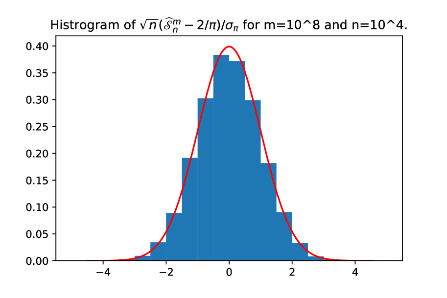
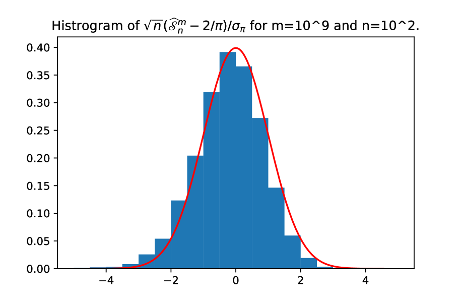
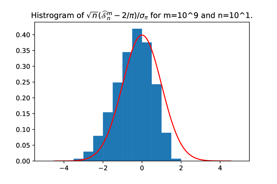
Figure 2: Empirical distribution of standardized ${\widehat{\mathscr{S}}_{n}^{m}}$ for different values of $r$, $m$ and $n$. The red line corresponds to the density of the standard normal distribution. In the left-hand side $r=0.1$, $m=10^{8}$ and $n=10^{4}$. In the center $r=0.4$, $m=10^{9}$ and $n=10^{2}$. In the right-hand side $r=0.45$, $m=10^{9}$ and $n=10^{2}$.

7.2 Experiments under $\mathbf{H_{1}}$

We have performed simulations for the parameter $r$ taking values in $\{0.6,0.75,0.9\}$ and for levels of confidence $q=0.1$ and $q=0.05$. Just as before, for each value of $r$, we have generated $10^{4}$ independent samples with sizes from $m=10^{5}$ up to $m=10^{8}$, and to study the respective effects of $m$ and $n$, for each sample size $m$ we have made the number of time steps $n$ vary from $n=10^{1}$ up to $n=10^{4}$.

Under $\mathbf{H_{1}}$ the empirical rejection rate is expected to be close to $1$. For $n=10^{3}$ it is exactly what our numerical experiments show. Nevertheless, under $\mathbf{H_{0}}$, the choice $n=10^{3}$ led to very poor results for $r\sim 0.5$, this motivate us to use smaller values of $n$.

In Tables 2(a) and 2(b) we report the empirical rejection rates for different values of $r$ and $q$ when $n<10^{3}$. Notice the change of regime between $n=10^{1}$ and $n=10^{2}$. When $r$ is close to the limit case $0.5$ we observe a bigger ‘type 2’ error.

As a complement, Table 3 shows values taken by the empirical second moment of $X$. Since we are under $\mathbf{H_{1}}$, we know that $\mathbb{E}\left(X^{2}\right)~{}=~{}\infty$. However, it is not so obvious that this information could suffice to decide that the second moment is infinite. More striking, in this case, the empirical second moment is not a reliable indicator of the infiniteness of $\mathbb{E}\left(X^{2}\right)$, regardless the size of the sample. However, even when $r=0.6$, the empirical rejection rates of our test are close to $1$ under $\mathbf{H_{1}}$. This seems to illustrate the relevance of our test to detect infinite expectations.

$r$	$n=10^{1}$	$n=10^{2}$
$0.6$	$0.194$	$0.761$
$0.75$	$0.268$	$0.950$
$0.9$	$0.340$	$0.987$

(a) $q=0.1$.

$r$	$n=10^{1}$	$n=10^{2}$
$0.6$	$0.123$	$0.712$
$0.75$	$0.189$	$0.934$
$0.9$	$0.251$	$0.984$

(b) $q=0.05$.

Table 2: Values of the empirical rejection rate (ERR) of the $\widehat{\mathscr{S}}_{n}^{m}$-test for $m=10^{8}$ for different values of $r$ under $\mathbf{H_{1}}$ and different values of $q$.

	$m$
Statistic	$10^{5}$	$10^{6}$	$10^{7}$	$10^{8}$
Mean of $\hat{M}_{2}$	$3.07\times 10^{2}$	$5.51\times 10^{2}$	$5.36\times 10^{2}$	$8.54\times 10^{2}$
Std. Deviation of $\hat{M}_{2}$	$1.04\times 10^{4}$	$1.23\times 10^{4}$	$6.48\times 10^{3}$	$1.31\times 10^{4}$
Min of $\hat{M}_{2}$	$2.00\times 10^{1}$	$3.28\times 10^{1}$	$5.30\times 10^{1}$	$9.05\times 10^{1}$
Max of $\hat{M}_{2}$	$9.76\times 10^{5}$	$7.68\times 10^{5}$	$4.44\times 10^{5}$	$9.70\times 10^{5}$
Quantile$(0.95)$ of $\hat{M}_{2}$	$3.09\times 10^{2}$	$5.68\times 10^{2}$	$8.72\times 10^{2}$	$1.31\times 10^{3}$
Quantile$(0.99)$ of $\hat{M}_{2}$	$1.80\times 10^{3}$	$3.44\times 10^{3}$	$5.03\times 10^{3}$	$7.67\times 10^{3}$

Table 3: Statistics of the empirical second moment computed in $10000$ scenarios for $r=0.6$. The sample sizes vary from $10^{5}$ to $10^{8}$.

7.3 Numerical experiments under weak dependence

The objective of this section is to show we can extend our test to some cases of weakly dependent data. Certainly, extra assumptions are necessary to obtain functional limit theorems by using the $J_{1}$-topology as in Theorem 2.4: For example, Avram and Taqqu [2], show that the $J_{1}$-weak convergence of normalized sums cannot hold for the classes of dependent random variables they consider.

Let us exhibit some sufficient conditions to replace the independency condition in Theorem 4.3. Assume that the sample is stationary, $r$-dependent and satisfy the two following conditions:

$$\sup\left\{|\operatorname{Corr}(f,g)|:\operatorname{real}f\in L^{2}(\sigma(X_{1})),\operatorname{real}g\in L^{2}(\sigma(X_{2},X_{3},\ldots))\right\}<1$$ (7.1)

and

$$\left(\forall\epsilon>0,\,\forall j=2,\ldots,k\right)\;\;\lim_{m\to\infty}\mathbb{P}\left(|X_{j}|>\epsilon c_{m}/|X_{1}|>\epsilon c_{m}\right)=0.$$ (7.2)

Let us start with adapting the proof of Proposition 4.1 to this setting. First, if $X$ is in the domain of attraction of the normal law, in view of (7.1) Corollary 1.1 in Shao [14] implies that $(S_{\lfloor mt\rfloor}-\mu_{n})/c_{m}$ converges to a scaled Brownian motion, from which $Z^{m}$ converges to a Brownian bridge. Second, if $X$ belongs to the domain of attraction of a stable law, under (7.2) Corollary 1.4 in Tyran-Kamińska [17] states that $(S_{\lfloor mt\rfloor}-\mu_{m})/c_{m}$ converges in distribution to a $\alpha$-stable random process, from which $Z^{m}$ converges in distribution to a $\alpha$-stable bridge. The rest of the arguments in the proof of Proposition 4.1 do not rely on the independency hypothesis.

Let us now turn to Proposition 4.2. Assume that $X$ is in the domain of attraction of the normal law. In view of (7.1) $Z^{m}$ converges to a Brownian bridge. Therefore, under $\mathbf{H_{0}}$,

$$\left|\mathbb{E}\left[\psi\left(\frac{\sqrt{n}}{\sigma_{\pi}}({\widehat{\mathscr{S}}_{n}^{m}}-\frac{2}{\pi})\right)\right]-\mathbb{E}\left[\psi\left(\frac{\sqrt{n}}{\sigma_{\pi}}(\widehat{\mathscr{S}}_{n}(Z)-\frac{2}{\pi})\right)\right]\right|,$$

converges to zero, for every fixed $n$, as $m$ goes to infinity. All the other arguments in the proof of Proposition 4.2 remain valid in this weak dependence setting.

We thus have shown one possible extension for Theorem 4.3 to samples of non-independent random variables.

To illustrate the behavior of the test for non-independent random variables, we consider a sequence $Y_{2},Y_{3},\ldots,Y_{m}$ of $1$-dependent random variables constructed as follows. First, we generate a sample $X_{1},\ldots,X_{m}$ of independent copies of  $|G|^{-r}$ where $G\sim\mathcal{N}(0,1)$, and then

$$Y_{k}=\frac{X_{k-1}}{X_{k-1}+1}X_{k}.$$ (7.3)

Second, we apply our methodology to $Y_{2},\ldots,Y_{m}$ for $r=0.3$ and $r=0.75$. Just as above we consider $10^{4}$ scenarios.

For $r=0.3$, $\mathbf{H_{0}}$ holds and the experiment shows that as $m$ increases the empirical rejections rates tend to the theoretical ones, for example for $q=0.1$, $m=10^{8}$ and $n=10^{3}$, the empirical rejection rate is $0.11$. As in the i.i.d. case we also observe that the performance of the methodology decreases when $n$ becomes too large.

For $r=0.75$, that is, under $\mathbf{H_{1}}$, smaller values of $n$ leads to bigger ‘type 2’ error. Nevertheless, for $n=10^{2}$ we already observe empirical rejection rates close to 1.

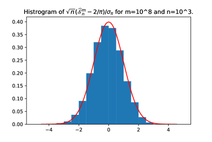
Figure 3: Empirical distribution of standardized ${\widehat{\mathscr{S}}_{n}^{m}}$ for the variables $Y_{k}$ defined in (7.3). The red line corresponds to the density of the standard normal distribution.

8 Conclusion

Inspired by Barndorff-Nielsen and Shephard’s methodology to test the existence of jumps in the trajectories of certain semimartingales, we have built an statistical test to determine if a given random variable $X$ belongs to the domain of attraction of the Gaussian law or of another stable law. This statistical test allows us to give a partial answer to the ill-posed (but important in practice) problem of testing the finiteness of moments of an observed random variable.

So far, our methodology is based on asymptotic results. For the purpose of practical applications it would be interesting to obtain a non-asymptotic version of our test or, at least, to obtain theoretical results on suitable dependences between the parameters $m$ and $n$ which guarantee that our hypothesis test is reliable. To obtain accurate estimates w.r.t. $m$ and $n$ for $\mathbb{P}\left(C_{n,m}|H_{0}\right)$ and $\mathbb{P}\left(C_{n,m}|H_{1}\right)=1$ (which supposes to obtain non asymptotic estimates precising the CLT for $\widehat{\mathscr{S}}_{n}^{m}$) the calculations appear to be heavy, lengthy and very technical. We hope to be able to obtain satisfying results in the next future.

Acknowledgment:

The two authors thank the referees of a first version of this paper for their useful suggestions to improve the overall organisation of the manuscript and to clarify some mathematical issues.

The first author is also grateful to Karine Bertin and Joaquin Fontbona for some helpfull discussions and comments on a previous version of this work.

Appendix A An elementary lemma on Gaussian distributions

In the proof below of the inequalities (6.8) and (6.9) we use the following elementary property of standard Gaussian laws. Recall that at the beginning of Section 6.4 the function $q$ was defined as

$$q(x,a,b)=|x-a||x-b|-|a||b|.$$

Let $\phi$, $\Phi$ respectively denote the density and the cumulative distribution function of a standard Gaussian random variable. In the computations below we will use the following elementary equalities that hold for any $x\in\mathbb{R}$ :

$$\int_{-\infty}^{\infty}\operatorname{sgn}(x-z_{1})~{}\phi(z_{1})~{}dz_{1}=2\Phi(x)-1,$$ (A.1)

$$\int_{-\infty}^{\infty}|x-z_{2}|~{}\phi(z_{2})~{}dz_{2}=2x\Phi(x)-x+2\phi(x),$$ (A.2)

and

$$\int_{-\infty}^{\infty}\int_{-\infty}^{\infty}q(x,z_{3},z_{4})~{}\phi(z_{3})~{}\phi(z_{4})~{}dz_{3}~{}dz_{4}=\left(2x\Phi(x)-x+2\phi(x)\right)^{2}-\frac{2}{\pi}.$$ (A.3)

A.1 Proof of Inequality (6.8)

Let $f(x,z_{1},z_{2},z_{3},z_{4})$ be defined as

$$f(x,z_{1},z_{2},z_{3},z_{4}):=q(x,z_{1},z_{2})q(x,z_{3},z_{4}).$$

Then

$$D_{-}f(x,z_{1},z_{2},z_{3},z_{4})=D_{-}q(x,z_{1},z_{2})q(x,z_{3},z_{4})+q(x,z_{1},z_{2})D_{-}q(x,z_{3},z_{4}),$$

and

$$D^{2}f(dx,z_{1},z_{2},z_{3},z_{4}) =f^{\prime\prime}(x,z_{1},z_{2},z_{3},z_{4})dx$$

$$\quad+2|z_{1}-z_{2}|q(z_{1},z_{3},z_{4})\delta_{z_{1}}(dx)+2|z_{2}-z_{1}|q(z_{2},z_{3},z_{4})\delta_{z_{2}}(dx)$$

$$\quad+2|z_{3}-z_{4}|q(z_{3},z_{1},z_{2})\delta_{z_{3}}(dx)+2|z_{4}-z_{3}|q(z_{4},z_{1},z_{2})\delta_{z_{4}}(dx),$$

where

$$f^{\prime\prime}(x,z_{1},z_{2},z_{3},z_{4}) =2\left[\operatorname{sgn}(x-z_{1})|x-z_{2}|+|x-z_{1}|\operatorname{sgn}(x-z_{2})\right]$$

$$\quad\times\left[\operatorname{sgn}(x-z_{3})|x-z_{4}|+|x-z_{3}|\operatorname{sgn}(x-z_{4})\right]$$

$$\quad+2\operatorname{sgn}(x-z_{1})\operatorname{sgn}(x-z_{2})q(x,z_{3},z_{4})$$

$$\quad+2\operatorname{sgn}(x-z_{3})\operatorname{sgn}(x-z_{4})q(x,z_{1},z_{2}).$$

It is then easy to check that the conditions 1-4 4 of Proposition 6.4 hold true.

It remains to check that conditions 5’ and 6’ of Proposition 6.4 also hold true. We use the same notation as in the aforementioned proposition. Observe that

$$h_{0}(x) =\mathbb{E}\left[f^{\prime\prime}(x,G_{i},G_{i+1},G_{k},G_{k+1})\right]$$

$$=\int_{-\infty}^{\infty}\int_{-\infty}^{\infty}\int_{-\infty}^{\infty}\int_{-\infty}^{\infty}f^{\prime\prime}(x,z_{1},z_{2},z_{3},z_{4})\phi(z_{1})\phi(z_{2})\phi(z_{3})\phi(z_{4})dz_{1}dz_{2}dz_{3}dz_{4}$$

$$=8\left(\int_{-\infty}^{\infty}\operatorname{sgn}(x-z_{1})\phi(z_{1})dz_{1}\right)^{2}\left(\int_{-\infty}^{\infty}|x-z_{2}|\phi(z_{2})dz_{2}\right)^{2}$$

$$\quad+4\left(\int_{-\infty}^{\infty}\operatorname{sgn}(x-z_{1})\phi(z_{1})dz_{1}\right)^{2}\int_{-\infty}^{\infty}\int_{-\infty}^{\infty}q(x,z_{3},z_{4})\phi(z_{3})\phi(z_{4})dz_{3}dz_{4}.$$

In view of equalities (A.1), (A.2) and (A.3) a straightforward computation leads to

$$h_{0}(x) =12\left(2\Phi(x)-1\right)^{2}\left(2x\Phi(x)-x+2\phi(x)\right)^{2}-\frac{8}{\pi}\left(2\Phi(x)-1\right)^{2}.$$

It is clear that $h_{0}(0)=0$ and also that $h$ is smooth enough to satisfy Condition 5’ in Proposition 6.4.

On the other hand, the weights of the singular part of $D^{2}f(dx,z_{1},z_{2},z_{3},z_{4})$ are given by

$$\gamma^{1}_{z} =2|z_{1}-z_{2}|q(z_{1},z_{3},z_{4}), \gamma^{2}_{z} =2|z_{2}-z_{1}|q(z_{2},z_{3},z_{4}),$$

$$\gamma^{3}_{z} =2|z_{3}-z_{4}|q(z_{3},z_{1},z_{2}), \gamma^{4}_{z} =2|z_{4}-z_{3}|q(z_{4},z_{1},z_{2}).$$

Since $G_{i},G_{i+1},G_{k},G_{k+1}$ are i.i.d. it follows

$$h_{1}(x) =\left(\int_{-\infty}^{\infty}\int_{-\infty}^{\infty}\int_{-\infty}^{\infty}|x-z_{2}|q(x,z_{3},z_{4})\phi(z_{2})\phi(z_{3})\phi(z_{4})dz_{2}dz_{3}dz_{4}\right)\phi(x)$$

$$=\left(\int_{-\infty}^{\infty}|x-z_{2}|\phi(z_{2})dz_{2}\right)\left(\int_{-\infty}^{\infty}\int_{-\infty}^{\infty}q(x,z_{3},z_{4})\phi(z_{3})\phi(z_{4})dz_{3}dz_{4}\right)\phi(x)$$

$$=\left(2x\Phi(x)-x+2\phi(x)\right)\left(\left(2x\Phi(x)-x+2\phi(x)\right)^{2}-\frac{2}{\pi}\right)\phi(x).$$

Notice that $h_{1}$ is $\mathcal{C}^{\infty}$, and its derivatives have polynomial growth, therefore $h_{1}$ satisfies Condition 6’ in Proposition 6.4.

Since $G_{i},G_{i+1},G_{k},G_{k+1}$ are identically distributed, one has that $h_{2}(x)=h_{3}(x)=h_{4}(x)=h_{1}(x)$, and therefore $h_{2},h_{3}$ and $h_{4}$ also satisfy Condition 6’ in Proposition 6.4.

Appendix B Proof of Inequality (6.9)

Notice that

$$\mathbb{E} \bigg{[}q(\bar{G}^{n\#},G_{i},G_{i+1})\left(|\frac{H_{i,k}}{n}||G_{k}+G_{k+1}-2\bar{G}^{n\#}|\right)\bigg{]}$$

$$\leq\mathbb{E}\bigg{[}q(\bar{G}^{n\#},G_{i},G_{i+1})\left(|\frac{G_{i}+G_{i+1}}{n}|+|\frac{G_{k}+G_{k+1}}{n}|\right)\left(|G_{k}+G_{k+1}|+2|\bar{G}^{n\#}|\right)\bigg{]}$$

$$=\mathbb{E}\bigg{[}q(\bar{G}^{n\#},G_{i},G_{i+1})|\frac{G_{i}+G_{i+1}}{n}||G_{k}+G_{k+1}|\bigg{]}+2\mathbb{E}\bigg{[}q(\bar{G}^{n\#},G_{i},G_{i+1})|\frac{G_{i}+G_{i+1}}{n}||\bar{G}^{n\#}|\bigg{]}$$

$$\quad+\mathbb{E}\bigg{[}q(\bar{G}^{n\#},G_{i},G_{i+1})\frac{|G_{k}+G_{k+1}|^{2}}{n}\bigg{]}+2\mathbb{E}\bigg{[}q(\bar{G}^{n\#},G_{i},G_{i+1})|\frac{G_{k}+G_{k+1}}{n}||\bar{G}^{n\#}|\bigg{]}$$

$$=:E_{1}+E_{2}+E_{3}+E_{4}.$$

We are now going to bound from above each $E_{i}$.

Again notice that $\bar{G}^{n\#}$ is equal in law to a Brownian motion $W$ at time $(n-4)/n^{2}$, from which

$$E_{2} =\frac{2}{n}\mathbb{E}\bigg{[}|G_{i}+G_{i+1}|q(W_{\frac{n-4}{n^{2}}},G_{i},G_{i+1})|W_{\frac{n-4}{n^{2}}}|\bigg{]},$$

We aim to apply the proposition 6.4 to the function

$$f(x,z_{1},z_{2}):=|z_{1}+z_{2}|~{}q(x,z_{1},z_{2})~{}|x|.$$

In this case, $z=(z_{1},z_{2})$. We have:

$$D_{-}f_{z}(x)=|z_{1}+z_{2}|D_{-}q(x,z_{1},z_{2})|x|+|z_{1}+z_{2}|q(x,z_{1},z_{2})\operatorname{sgn}(x),$$

and

$$D^{2}f_{z}(dx) =f_{z}^{\prime\prime}(x)dx+2|z_{1}+z_{2}||z_{1}-z_{2}|\delta_{z_{1}}(dx)+2|z_{1}+z_{2}||z_{2}-z_{1}|\delta_{z_{2}}(dx),$$

where

$$f_{z}^{\prime\prime}(x) =2|z_{1}+z_{2}|\left(\operatorname{sgn}(x-z_{1})|x-z_{2}|+|x-z_{1}|\operatorname{sgn}(x-z_{2})\right)\operatorname{sgn}(x)$$

$$\quad+2|z_{1}+z_{2}|\operatorname{sgn}(x-z_{1})\operatorname{sgn}(x-z_{2}).$$

We now show that for $i=0,1,2$, the functions $t\to\mathbb{E}\left[h_{i}(W_{t})\right]$ are bounded for $t$ in a neighborhood of  $0$.

Indeed,

$$|h_{0}(x)| =|\mathbb{E}\left[f_{G}^{\prime\prime}(x)\right]|$$

$$\leq\int_{\mathbb{R}^{2}}\left(2|z_{1}+z_{2}|\left(|x-z_{2}|+|x-z_{1}|\right)+2|z_{1}+z_{2}|\right)\phi(z_{1})\phi(z_{2})dz_{1}dz_{2}$$

$$\leq\int_{\mathbb{R}^{2}}\left((z_{1}+z_{2})^{2}+\left(|x-z_{2}|+|x-z_{1}|\right)^{2}+2|z_{1}+z_{2}|\right)\phi(z_{1})\phi(z_{2})dz_{1}dz_{2}$$

$$=2+\int_{\mathbb{R}^{2}}\left(\left(x-z_{2}\right)^{2}+2|x-z_{2}||x-z_{1}|+\left(x-z_{1}\right)^{2}\right)\phi(z_{1})\phi(z_{2})dz_{1}dz_{2}+\frac{4}{\sqrt{\pi}}$$

$$=2+2+2x^{2}+2\left(\int_{-\infty}^{\infty}|x-z_{1}|\phi(z_{1})dz_{1}\right)\left(\int_{-\infty}^{\infty}|x-z_{2}|\phi(z_{2})dz_{1}dz_{2}\right)+\frac{4}{\sqrt{\pi}}$$

$$=4+2x^{2}+2\left(2x\Phi(x)-x+2\phi(x)\right)^{2}+\frac{4}{\sqrt{\pi}}$$

$$\leq C_{1}+C_{2}|x|+C_{3}x^{2}.$$

Hence,

$$\mathbb{E}\left[h_{0}(W_{t})\right]\leq C_{1}+C_{2}\mathbb{E}\left[|W_{t}|\right]+C_{3}\mathbb{E}\left[W_{t}^{2}\right]=C_{1}+C_{2}\sqrt{t}+C_{3}t.$$

In particular, Condition 5 in Proposition 6.4 holds true.

Similarly,

$$|h_{1}(x)|=\left|2\left(\int_{-\infty}^{\infty}|x^{2}-z_{2}^{2}|\phi(z_{2})dz_{2}\right)\phi(x)\right|\leq 2\left(x^{2}+1\right).$$

Due to the symmetries of the weights $h_{1}=h_{2}$, and therefore for $i=1,2$

$$\mathbb{E}\left[h_{i}(W_{t})\right]\leq C_{1}+C_{2}\mathbb{E}\left[W_{t}^{2}\right]=C_{1}+C_{2}t,$$

and Condition 6 in 6.4 also holds true. We therefore are in a position to use Proposition 6.4 and get

$$\mathbb{E}\bigg{[}|G_{i}+G_{i+1}|q(W_{\frac{n-4}{n^{2}}},G_{i},G_{i+1})|W_{\frac{n-4}{n^{2}}}|\bigg{]}\leq C\frac{n-4}{n^{2}},$$

from which

$$E_{2}\leq\frac{C(n-4)}{n^{3}}.$$

Similar arguments allow us to show that $E_{i}\leq\frac{C(n-4)}{n^{3}}$ for $i=1,3,4$. That ends the proof of (6.9).

References

- [1] Yacine Aït-Sahalia and Jean Jacod. Testing for jumps in a discretely observed process. The Annals of Statistics, 37(1):184–222, 02 2009.
- [2] Florin Avram and Murad S. Taqqu. Weak Convergence of Sums of Moving Averages in the -Stable Domain of Attraction. The Annals of Probability, 20(1):483 – 503, 1992.
- [3] Ole E Barndorff-Nielsen and Neil Shephard. Econometrics of testing for jumps in financial economics using bipower variation. Journal of financial Econometrics, 4(1):1–30, 2006.
- [4] Jean Bertoin. Lévy Processes, volume 121. Cambridge university press, 1998.
- [5] Paul Embrechts and Charles M Goldie. On closure and factorization properties of subexponential and related distributions. Journal of the Australian Mathematical Society, 29(2):243–256, 1980.
- [6] Paul Embrechts, Claudia Klüppelberg, and Thomas Mikosch. Modelling Extremal Events: for Insurance and Finance. Stochastic Modelling and Applied Probability. Springer Berlin Heidelberg, 1997.
- [7] William Feller. An Introduction to Probability Theory and Its Applications. Number v. 2 in An Introduction to Probability Theory and Its Applications. Wiley, 1971.
- [8] Doyle L. Hawkins. Can the finiteness of a mean be tested? Statistics & Probability Letters, 32(3):273 – 277, 1997.
- [9] Wassily Hoeffding and Herbert Robbins. The central limit theorem for dependent random variables. Duke Math. J., 15(3):773–780, 09 1948.
- [10] Jean Jacod and Albert Shiryaev. Limit Theorems for Stochastic Processes, volume 288. Springer Science & Business Media, 2013.
- [11] Jana Jurečková and Jan Picek. A class of tests on the tail index. Extremes, 4(2):165–183, 2001.
- [12] Natalia Markovich. Nonparametric Analysis of Univariate Heavy-tailed data: Research and Practice. John Wiley & Sons, 2008.
- [13] Héctor Olivero and Denis Talay. Supplementary material to “a hypothesis test for the domain of attraction of a random variable”. https://hal.science/hal-04266438.
- [14] Shao Qiman. An invariance principle for stationary p-mixing sequences with infinite variance. Chinese Annals of Mathematics B, 14(1):27–42, 1993.
- [15] Alain-Sol Sznitman. Topics in propagation of chaos. In École d’Été de Probabilités de Saint-Flour XIX—1989, volume 1464 of Lecture Notes in Math., pages 165–251. Springer, Berlin, 1991.
- [16] Denis Talay and Milica Tomasevic. A stochastic particle method to solve the parabolic-parabolic Keller-Segel system: an algorithmic and numerical study. 2022. Submitted for publication.
- [17] Marta Tyran-Kamińska. Convergence to lévy stable processes under some weak dependence conditions. Stochastic Processes and their Applications, 120(9):1629–1650, 2010.
- [18] Ward Whitt. Stochastic-process Limits: An Introduction to Stochastic-process Limits and their Application to Queues. Springer Science & Business Media, 2002.