Tunable Complexity Benchmarks for Evaluating Physics-Informed Neural Networks on Coupled Ordinary Differential Equations

Abstract

In this work, we assess the ability of physics-informed neural networks (PINNs) to solve increasingly-complex coupled ordinary differential equations (ODEs). We focus on a pair of benchmarks: discretized partial differential equations and harmonic oscillators, each of which has a tunable parameter that controls its complexity. Even by varying network architecture and applying a state-of-the-art training method that accounts for “difficult” training regions, we show that PINNs eventually fail to produce correct solutions to these benchmarks as their complexity—the number of equations and the size of time domain—increases. We identify several reasons why this may be the case, including insufficient network capacity, poor conditioning of the ODEs, and high local curvature, as measured by the Laplacian of the PINN loss.

1 Introduction

In recent years, there has been much interest in using machine learning (ML) models to approximate systems governed by mechanistic dynamics (Willard et al. 2020; Karniadakis et al. 2021). This includes rapid forward simulations and the ability to determine unknown components of dynamics via solution of inverse problems. Typically, these physics-based ML models incorporate a priori knowledge of the system to be modeled—via a black-box simulation environment or an explicit system of differential equations (DEs). In this work, we analyze a popular approach to the latter strategy: physics-informed neural networks (PINNs) (Raissi, Perdikaris, and Karniadakis 2019). PINNs incorporate DEs as physics-based regularizers in the objective function of a neural network (i.e., soft constraints) along with terms associated with initial and boundary conditions. This is a straightforward approach to incorporating known dynamics into neural networks and showed early success (McClenny and Braga-Neto 2020; Lu et al. 2021), but recent results (McClenny and Braga-Neto 2020; Krishnapriyan et al. 2021; Wang, Teng, and Perdikaris 2021; Wang, Yu, and Perdikaris 2022) highlight difficulties that PINNs face due to their complex objectives. Our analysis builds upon these latter efforts, focusing on representing coupled systems of ordinary differential equations (ODEs).

ODE systems, or differential equations with a single independent variable and one or more dependent variables, arise in a number of use cases. These include modeling reaction-diffusion processes in synthetic biology (Singhal et al. 2021) and chemical kinetics (Ji et al. 2021), as well as solving partial differential equations (PDEs) via the method of lines (Verwer and Sanz-Serna 1984). This leads, for example, to applications in fluid mechanics like Burgers’ equation (Zogheib et al. 2021) and condensed matter physics such as lattice dynamics (Chow, Mallet-Paret, and Van Vleck 1996).

Systems of ODEs vary in complexity based on domain size, number of equations being modeled, and problem stiffness. These challenges occur regularly—for example, when discretizing PDEs into coupled ODEs, the number of ODEs scales with discretization granularity. This is a computational bottleneck in higher-fidelity simulations. Due to the ubiquity of these systems, it is natural to explore how effectively PINNs solve them, especially as their complexities increase. Similar work was performed by (Krishnapriyan et al. 2021), who use underlying PDE parameters such as convection coefficients as proxies for the complexity of the learning problem, and show that PINNs fail to solve these problems as the complexity increases.

In this paper, we review the formulation of PINNs (Section 2.1) and introduce two problems that involve systems of coupled ODEs (Section 2.3). Each problem is characterized by a tunable “complexity”. We then demonstrate that PINNs, even with the use of a state-of-the-art training method, fail to produce correct solutions to the system of ODEs (as indicated by a classical ODE solver) as the complexity of the problem increases (Section 3). We then link the intuitive complexity of the problem with a quantitative characterization of the difficulty via the Laplacian of the PINN learning problem.

2 Approach

2.1 Physics-Informed Neural Networks

PINNs (Raissi, Perdikaris, and Karniadakis 2019) are neural networks with weights trained such that the network satisfies a differential equation. The use of a neural network to satisfy a DE is motivated by the universal approximation theorem; however, this theorem does not guarantee that a specific optimization procedure will yield a network satisfying the DE. (Shin 2020) showed that, for certain categories of PDE, as the amount of available data increases, the PINN learning problem will converge to a solution to the PDE.

Due to the overhead of training, solving a DE with a PINN takes longer than using a classical numerical method. Unlike classical methods, however, PINNs are easily extended to inverse problems—i.e., given a partially-specified governing equation and some data, recover the full governing equation. Furthermore, PINNs do not require a mesh, which enables efficient application to new problems. The forward prediction setting, which we consider here, is a different use-case than many ML applications, in that the training signal uses a DE (or system of DEs), rather than a labelled dataset.

To define PINNs, consider a general ODE that determines function $\mathbf{u}:\mathbb{R}\to\mathbb{R}^{N}$:

$$\mathcal{N}(\mathbf{u})(t) = 0,\,\,\,\,\,t\in(0,T)$$

$$\mathcal{I}(\mathbf{u})(t) = 0,\,\,\,\,\,t=0,$$

where $\mathcal{N}$ is a differential operator, and $\mathcal{I}$ captures deviation from prespecified initial conditions. For the first-order DEs considered here, $\mathcal{I}(\mathbf{u})(t)=\mathbf{u}(t)-\mathbf{u}_{0}$, where $\mathbf{u}_{0}$ is fixed. Then a PINN $\hat{\mathbf{u}}_{w}:\mathbb{R}\to\mathbb{R}^{N}$ is a neural network parameterized by a weight vector $w\in\mathbb{R}^{M}$ that satisfies

$$\min_{w}L(w)=\sum_{t_{d}\in\mathcal{T}}||\mathcal{N}(\hat{\mathbf{u}}_{w})(t_{d})||^{2}+\nu_{\mathcal{I}}||\mathcal{I}(\mathbf{\hat{u}}_{w})(0)||^{2},$$ (1)

where $\nu_{\mathcal{I}}>0$ weights the initial condition components and $\mathcal{T}=\{t_{1},\ldots,t_{D}\}\subseteq(0,T)$ is the set of training points. The PINN literature typically refers to the loss term involving the differential operator $\mathcal{N}$ as the residual loss.

The PINN loss $L(w)$ may be minimized with first-order methods like Adam (Kingma and Ba 2014). Unlike many other ML settings, it includes derivatives of $\hat{\mathbf{u}}_{w}$ with respect to its input $t$. These may be calculated using the same automatic differentiation procedures (Baydin et al. 2017) used to calculate loss gradients with respect to network weights, but this means that the weight update of a PINN loss function contains second- and higher-order derivatives (a gradient calculation with respect to $w$, combined with derivatives with respect to $t$ based on the DE).

In practice, we often solve a modified formulation of Equation 2, introduced by (McClenny and Braga-Neto 2020):

$$\min_{w}\max_{\lambda}L(w,\lambda)$$ (2)

where

$$L(w,\lambda) = \frac{1}{|\mathcal{T}|}\sum_{t_{d}\in\mathcal{T}}\mu(\lambda_{d})||\mathcal{N}(\mathbf{\hat{u}}_{w})(t_{d})||^{2}$$

$$+\mu(\lambda_{0})\nu_{\mathcal{I}}||\mathcal{I}(\mathbf{\hat{u}}_{w})(0)||^{2},$$

where $\lambda\in\mathbb{R}^{D+1}_{\geq 0}$ are attention weights associated with each point $t_{d}\in\{0\}\cup\mathcal{T}$, and $\mu:\mathbb{R}^{+}\to\mathbb{R}^{+}$ is a masking function required to be differentiable, non-negative, and strictly increasing. This problem can be solved with a joint gradient ascent (for attention weights $\lambda$) and descent (for PINN weights $w$) procedure.

(Krishnapriyan et al. 2021) observe that the PINN learning problem can be ill-conditioned due to the differential operator $\mathcal{N}$ in $L$. We continue this line of analysis by considering the Laplacian $\Delta L_{c}$ of a component $c$ (residual loss or initial condition loss) of $L$ with respect to the network weights $w$:

$$\Delta L_{c}(w)=\sum_{p}\partial_{w_{p},w_{p}}L_{c}(w),$$

where $L_{c}$ is the residual loss or the initial condition loss in Equation 1. The Laplacian’s magnitude measures the local size of the learning problem’s curvature. We evaluate the Laplacian by estimating the trace of the Hessian $\nabla^{2}L_{c}(w)$ using Hutchinson’s method (Yao et al. 2020):

$$\Delta L_{c}(w)=\mathrm{tr}\,\nabla^{2}L_{c}(w)=\mathbb{E}_{v}\{v^{T}[(\nabla^{2}L_{c})(w)]v\},$$

where $v\in\mathbb{R}^{M}$ has $iid$ components sampled from a Rademacher distribution, and the Hessian-vector products do not require the full Hessian (Pearlmutter 1994).

PINNs have primarily been used to solve and analyze PDEs rather than ODEs. This is partially because, unlike for PDEs (Brandstetter, Worrall, and Welling 2022), classical ODE solvers such as Runge-Kutta (Dormand and Prince 1980) are efficient for forward predictions of ODE systems. We focus here on forward prediction of ODEs because they represent the simplest-possible application domain of PINNs. PINN failures during forward prediction should be addressed to allow general use of PINNs in other settings like inverse problems and PDEs.

2.2 The pinn-jax library

PINN research has benefited from several open-source libraries, including DeepXDE (Lu et al. 2021), NeuralPDE.jl (Zubov et al. 2021), and TensorDiffEq (McClenny, Haile, and Braga-Neto 2021). DeepXDE in particular easily enables solving PINNs over irregular domain geometries. For this work, we implemented our PINNs in a new library, pinn-jax, which is built on the jax framework and uses flax for neural network layers and optax for optimization. The use of jax improves code performance and allows calculations to be run on CPUs/GPUs/TPUs as available, while preserving the flexibility to specify different ODEs and obtain their solutions via different PINN training strategies (e.g., different weighting schemes) and neural network architectures (e.g., multi-layer perceptrons (MLPs) and ResNets (He et al. 2016)).

As we consider scalar inputs for our networks, pinn-jax implements first-order loss derivatives with forward-mode automatic differentiation (the jacfwd function), and second-order loss derivatives with forward-over-forward-mode automatic differentiation. The vmap function enables efficient calculation of these derivatives over an entire batch of domain points. Calculation of Hessian-vector products to assess loss Laplacians $\Delta L_{c}$ is accomplished by composing the Jacobian-vector product function jvp with the gradient function grad. Although we focus on PINNs for ODEs, we note that pinn-jax also includes functionality for solving PDEs. In that component of the library, we use DeepXDE’s  (Lu et al. 2021) geometry module, which enables specification of and sampling from complex domains.

2.3 Benchmarks

After finding it difficult to train PINNs on a set of biological reaction equations, we decided to explore the broader problem of using PINNs to solve systems of ODEs. This resulted in the development of two benchmarks with parameterized complexity—one that scales the number of equations in the system (a discretized heat equation) and the other that defines complexity as a maximum simulation time (simple harmonic motion (SHM)). Each of our benchmarks has additional parameters (e.g., choice of initial conditions) that we do not vary in these results—our goal is to leave much fixed and explore the effect of increasing complexity on the ability of a PINN to solve these ODE systems.

Discretized heat equation

The heat equation, $\mathbf{u}_{t}=\Delta\textbf{u}$, is defined for a scalar field $u$ on the domain $(x,t)\in(0,1)\times(0,T)$. In particular, when sources are added to it, one obtains a broad family of reaction-diffusion systems applicable to lattice problems (Chow, Mallet-Paret, and Van Vleck 1996). Although the heat equation may be solved as a PDE with a PINN, here we explore how effectively PINNs solve it after it is discretized into a set of coupled ODEs. In particular, we apply the method of lines (Verwer and Sanz-Serna 1984) and discretize the spatial dimension into $N$ evenly-spaced points $x_{1},\ldots,x_{N}$, where $x_{n}=(n-1)\Delta x=(n-1)/(N-1)$, and then approximate the second derivative with a central finite difference. This yields the following coupled ODE, for a function $\mathbf{u}:\mathbb{R}\to\mathbb{R}^{N}$:

$$\dot{\mathbf{u}} = \mathbf{A}\mathbf{u}+\mathbf{f},\,\,\,\,t\in(0,T),$$

$$\mathbf{u}_{t=0} = [g(x_{1}),\ldots,g(x_{N})]^{T}$$

where the matrix $\mathbf{A}$ is given by

$$\mathbf{A}_{n,n} = -2(N-1)^{2}$$

$$\mathbf{A}_{n,n+1} = (N-1)^{2}$$

$$\mathbf{A}_{n+1,n} = (N-1)^{2}$$

$$\mathbf{A}_{n,n^{\prime}} = 0.$$

Further, $\mathbf{f}=(N-1)^{2}[u_{L}(t),0,\ldots,0,u_{R}(t)]^{T}$, $g$ specifies the initial condition, and $u_{L}$ and $u_{R}$ specify the boundary conditions on the left and right side, respectively, of the spatial domain $(0,1)$.

An example solution to this problem is shown in Figure 1. In this discretized formulation, the complexity of the problem is determined by the size of the discretization $N$. The discretized differential operator $\mathbf{A}$ couples each state variable $u_{n}$ to its spatially-adjacent variables $u_{n+1}$ and $u_{n-1}$.

As the number of discretized space-points $N$ increases, the coupled ODEs become more ill-conditioned. Specifically, as $\mathbf{A}$ is a symmetric tridiagonal Toeplitz matrix, it has a closed-form representation of its eigenvalues (Noschese, Pasquini, and Reichel 2013):

$$e_{n} = -2(N-1)^{2}(1-\cos(n\pi/(N+1))),$$

for $n=1,\ldots,N$.

In this case, the condition number is given by:

$$\kappa_{N}=\frac{|e_{N}|}{|e_{1}|}=\frac{1-\cos(N\pi/(N+1))}{1-\cos(\pi/(N+1))}$$

Since the condition number increases without bound as the discretization size $N$ increases, we have an explicit connection between an intuitive notion of complexity ($N$) and a more formal notion of complexity (the condition number of the matrix $\mathbf{A}$). Further details on this benchmark are found in Appendix A.

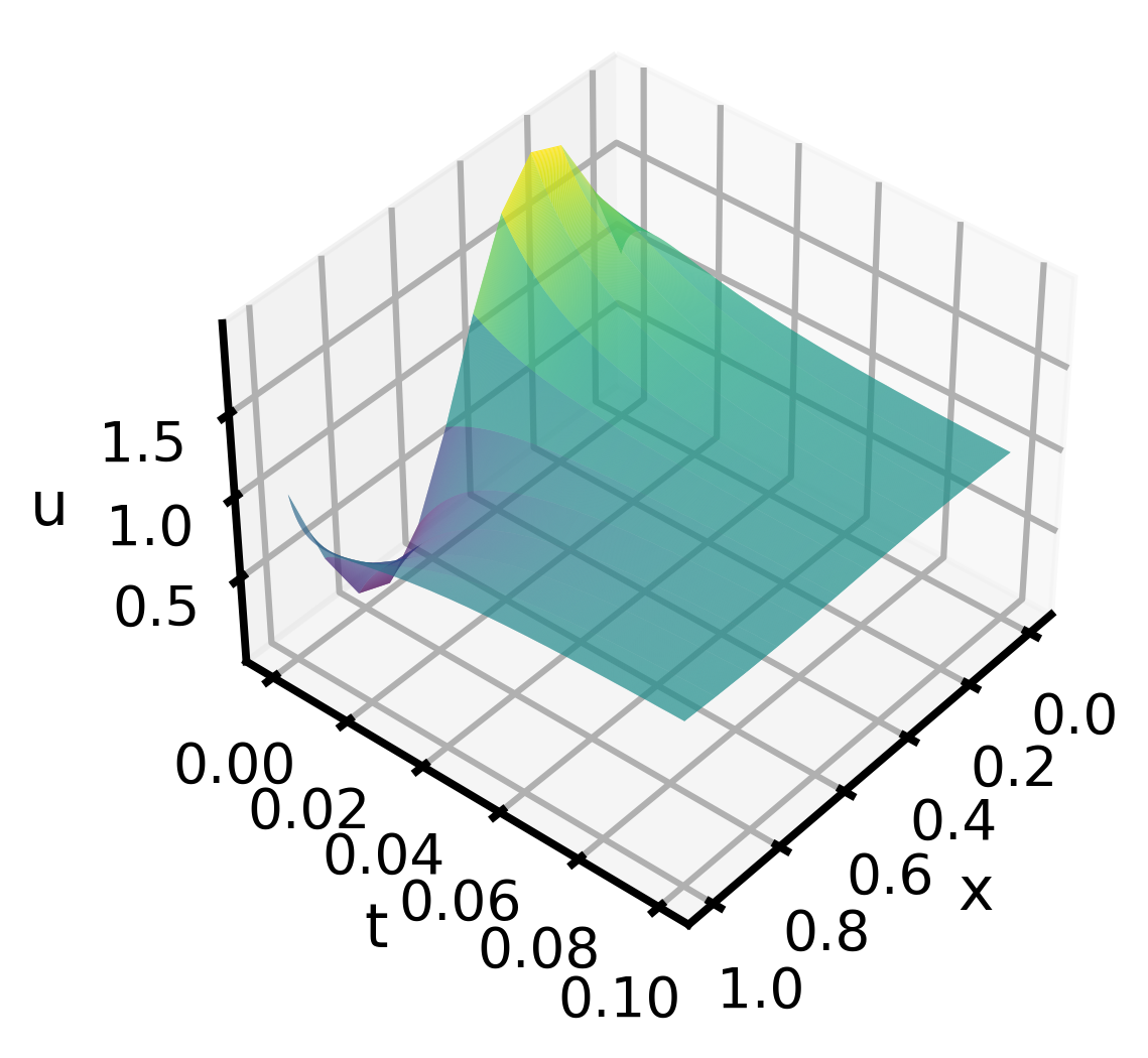
Figure 1: An example solution to the heat equation (Section 2.3). At $t=0$, the system has a sinusoidal shape; as $t$ increases, the solution decays to a constant value. As the discretization of the spatial dimension increases, the problem becomes more ill-conditioned.

Long time-horizon simple harmonic motion

We begin by considering a classic coupled ODE: simple harmonic motion (SHM), and we increase its complexity by evaluating it over increasingly large time domains. This ODE, for a function $\mathbf{u}:\mathbb{R}\to\mathbb{R}^{2}$, is specified by

$$\dot{\mathbf{u}} = \mathbf{A}\mathbf{u},\,\,\,\,\,\,\,\,\,\,t\in(0,T)$$

$$\mathbf{u}_{t=0} = \mathbf{u}_{0}$$

where the matrix $\mathbf{A}$ is given by $\mathbf{A}_{1,2}=-\omega$, $\mathbf{A}_{2,1}=\omega$, and $\mathbf{A}_{1,1}=\mathbf{A}_{2,2}=0$, for a frequency $\omega>0$. This problem has a closed-form solution in which $u_{1}$ and $u_{2}$ are sinusoidal, and a representative solution is shown in Figure 2. In this work, we use a fixed initial condition of $\mathbf{u}_{0}=[0,\pi/2]^{T}$ and a frequency of $\omega=1$.

When being solved by a PINN, the complexity of the ODE is determined by the size of the time domain $T$. Although the solution is periodic, we will show that PINNs fail to solve this ODE as $T$ increases in Section 3.3.

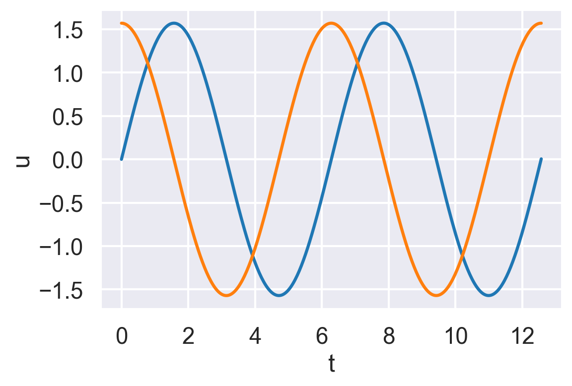
Figure 2: A solution to the SHM problem (Section 2.3); as the size of the time domain increases, the model becomes harder to solve with a PINN. The initial condition $\mathbf{u}_{0}=[0,\pi/2]^{T}$ was used with a maximum time of $T=4\pi$ and a frequency of $\omega=1$.

2.4 Related work

PINNs were introduced in (Raissi, Perdikaris, and Karniadakis 2019), and there has been a great deal of follow-on research. We focus on work that considers the PINN learning problem and recommend (Karniadakis et al. 2021) as an overview of the broader space of physics-informed ML.

Because the PINN formulation is end-to-end differentiable, it is easily modified—e.g., for uncertainty estimation of components (Yang, Meng, and Karniadakis 2021). Although a given trained network $\hat{\mathbf{u}}_{w}$ is valid only for a single instantiation of the DE, transfer learning approaches (Arthurs and King 2021) were shown to enable generalization over some spaces of parametrically-related equations.

(Wang, Teng, and Perdikaris 2021) showed that standard PINNs can fail to solve simple PDEs like the 2D Helmholtz equation with a known analytic solution. The PINN struggled with fitting this problem’s boundary condition, which the authors relate to underlying stiffness in the dynamics of the PINN training process. They suggest several heuristic strategies for mitigating this stiffness, including a learning rate annealing process and a novel network architecture. Similarly, (Maddu et al. 2022) use gradient uncertainties to adjust learning rates for PINNs.

In follow-on work (Wang, Yu, and Perdikaris 2022) analyzed the dynamics of the PINN learning problem through a neural tangent kernel (NTK) (Jacot, Gabriel, and Hongler 2018) perspective and found that components of the PINN loss function had different convergence rates. Most recently, (Wang, Sankaran, and Perdikaris 2022) proposed a time-weighted scheme for training PINNs that attempts to preserve physical causality in DEs, and (Daw et al. 2022) analyzed how PINNs can fail to propgate solutions across large time-domains.

(McClenny and Braga-Neto 2020) observed that different regions of the domain can be harder to solve and introduced a set of attention weights to allow the network to adaptively focus on difficult regions of the domain. In a later addition to their paper, they built from (Wang, Yu, and Perdikaris 2022) and conducted a NTK analysis of this modified loss function.

(Krishnapriyan et al. 2021) focused instead on the difficulties that follow from the presence of differential operators in the PINN loss function. This operator can lead to a poorly-conditioned loss function (as measured by local smoothness), which impairs the PINN’s ability to model simple PDEs like a reaction-diffusion model. (Krishnapriyan et al. 2021) also used Hessian-based information to analyze PINNs— specifically, they perturbed the PINN loss in directions defined by the top two principal eigenvectors of the Hessian. (Wang, Teng, and Perdikaris 2021) tracked the principal eigenvalue of the Hessian to define a time scale of training. Outside of work with PINNs, (Yao et al. 2020) analyze Hessian traces and spectral densities of feed-forward neural networks for computer vision problems, and (Yao et al. 2021) proposes a training scheme that uses an approximated Hessian diagonal to account for single-objective loss function curvature.

Similarly to our work, (Ji et al. 2021) noted that the PINNs defined by (Raissi, Perdikaris, and Karniadakis 2019) struggle when attempting to model stiff systems of ODEs for chemical kinetics models. They showed that the quasi-steady-state assumption, used to reduce the stiffness of a problem by assuming a zero concentration change rate for certain variables, can improve the accuracy of PINNs when the reduced system is used as the PINN loss $L(w)$. This approach showed promise for stiff systems, but will likely not mitigate the general challenge of ODE system complexity with increased problem size and coupling.

Although the classic PINN focuses on the strong formulation of a DE,  (Kharazmi, Zhang, and Karniadakis 2021) instead solved the weak formulation of a DE. Other extensions to the PINN learning problem came from (Yang, Zhang, and Karniadakis 2020), who incorporated a generative adversarial component into their PINN.

One of our benchmarks (Section 2.3) shows that the accuracy of a PINN breaks down as the size of the time domain $T$ increases. Prior work has considered similar settings for PINNs (Krishnapriyan et al. 2021; Meng et al. 2020) and operator-learning approaches (Wang and Perdikaris 2021), albeit focusing more on complicated PDEs. We show here that the challenge of using PINNs for long time-horizon forecasting exists even in the simplest ODEs.

3 Results

3.1 Evaluation procedure

In Table 1 in Appendix B, we show the network configurations and hyperparameters considered when training PINNs for each benchmark. All hidden layers had the same number of units (64 or 128) depending on the particular architecture, and ResNet models incorporate skip connections (He et al. 2016) between hidden layers. These network sizes are typical of those used in PINN literature (e.g., (Wang, Sankaran, and Perdikaris 2022; McClenny and Braga-Neto 2020; Maddu et al. 2022), which primarily consider networks with 4-5 layers and 20-100 hidden units).

We selected training points across the time domain as $\mathcal{T}=\{T/D,2T/D,\ldots,(D-1)T/D,T\}$, evaluation points as the midpoints of $\mathcal{T}$: $\mathcal{T}^{\prime}=\{(3T)/(2D),\ldots,(2D-1)T/(2D)\}$, and for each benchmark/complexity value pair we trained a total of 48 PINN configurations. All networks used $\tanh$ activation functions to ensure smoothness in the loss, and Table 2 in Appendix B includes benchmark-specific parameters.

3.2 Evaluation metrics

We evaluate PINN solutions via several methods. The primary approach is with the relative $\ell^{2}$ error of the PINN solution $\mathbf{\hat{u}}_{w}$ at the end of training vs. a solution $\mathbf{u}$ obtained with a classical ODE solver:

$$\mathrm{RelError}_{\mathcal{T^{\prime}}}(\mathbf{u},\mathbf{\hat{u}}_{w})=\sqrt{\frac{\sum_{t^{\prime}\in\mathcal{T}^{\prime}}||\mathbf{u}(t^{\prime})-\mathbf{\hat{u}}_{w}(t^{\prime})||^{2}}{\sum_{t^{\prime}\in\mathcal{T}^{\prime}}||\mathbf{u}(t^{\prime})||^{2}}},$$

where $\mathcal{T}^{\prime}\subseteq(0,T)$ is a set of evaluation collocation points distinct from the training points $\mathcal{T}$. Classical solver solutions are obtained with the solve_ivp function in scipy.integrate using RK45, the explicit Runge-Kutta method of order 5(4) (i.e., fourth-order accuracy with fifth-order local extrapolation) (Dormand and Prince 1980). In addition, we consider relative initial condition error

$$\mathrm{RelError}_{0}(\mathbf{u},\mathbf{\hat{u}}_{w})=\frac{||\mathbf{u}_{0}-\hat{\mathbf{u}}_{w}(0)||}{||\mathbf{u}_{0}||}.$$

As discussed in Section 2.1, we track the complexity of the PINN learning problem with the Laplacian of components of the PINN loss function. We also demonstrate that our notion of benchmark “complexity” or “difficulty” correlates with this measure of complexity for some benchmarks.

3.3 Relative error analysis

In Figure 3, we show that PINNs fail to solve the discretized heat equation problem (Section 2.3) as the discretization size $N$ increases. This happens across variations in network architecture and PINN formulation. Despite our normalization of the residual loss by the norm of the discretized differential operator, the uniform PINN formulation (Equation 1) fails to solve the problem, and the adaptive PINN (Equation 2) performs worse.

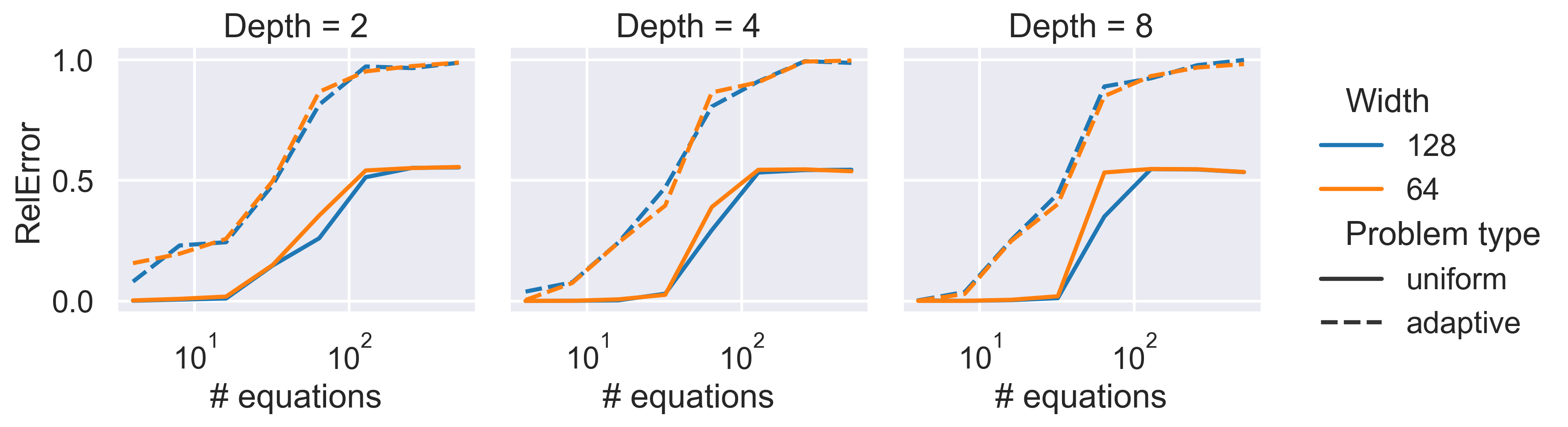
Figure 3: In the heat equation benchmark, all PINNs fail to solve the problem as dimensionality $N$ increases. Adaptive weighting in the domain (McClenny and Braga-Neto 2020) performs worse than uniform weighting—the weights $\lambda$ cannot mitigate the increase in ill-conditionedness of the problem. Interestingly, increasing network depth and width have little effect on the final relative error. Here we show relative error results for MLPs initiated with a learning rate of $10^{-3}$; results for other PINN configurations are comparable or worse.

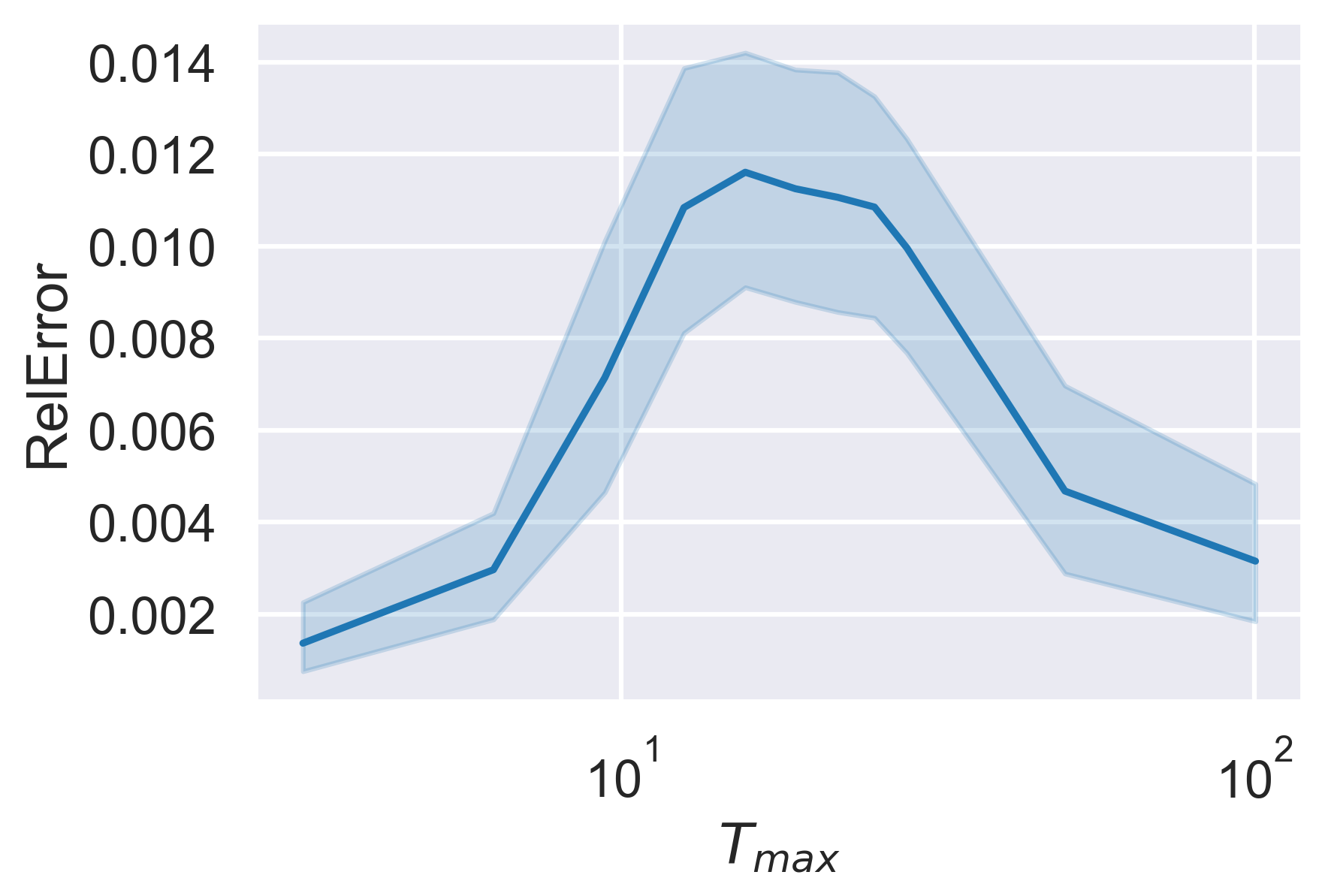
Figure 7: For the SHM problem, all PINNs are able to consistently minimize the relative initial condition error. Here we plot the final relative errors, averaged over all network configurations. Error bars indicate 95% confidence intervals for the estimate of the mean.

In Figure 4, we show that PINNs fail to solve the SHM problem (Section 2.3) as the maximum time $T$ of the domain increases. This happens despite our variations in network architecture and PINN formulation, as well as the fact that we increase the number of training points $D$ as the maximum time $T$ increases (Appendix B, Table 2). All configurations are able to effectively learn the problem’s initial condition—in Figure 7 in Appendix C, we show that the average relative errors for the initial condition do not exceed 0.02. In this problem, the adaptive weighting scheme (McClenny and Braga-Neto 2020) attains the lowest relative error but is still dependent on other hyperparameters.

In Figure 4 (SHM) but not Figure 3 (heat equation), deeper networks were able to solve more complex problems—although the high-end of time domain size still results in a failed PINN. This is likely not an indication that increased network depth is a solution, as the underlying phenomena has a simple periodic structure with fixed complexity. Thus, the PINN is not discovering the periodic structure in SHM and can only learn the DE’s behavior with very high-capacity networks. This works in this SHM setting, but will not scale to complex long-time horizon phenomena.

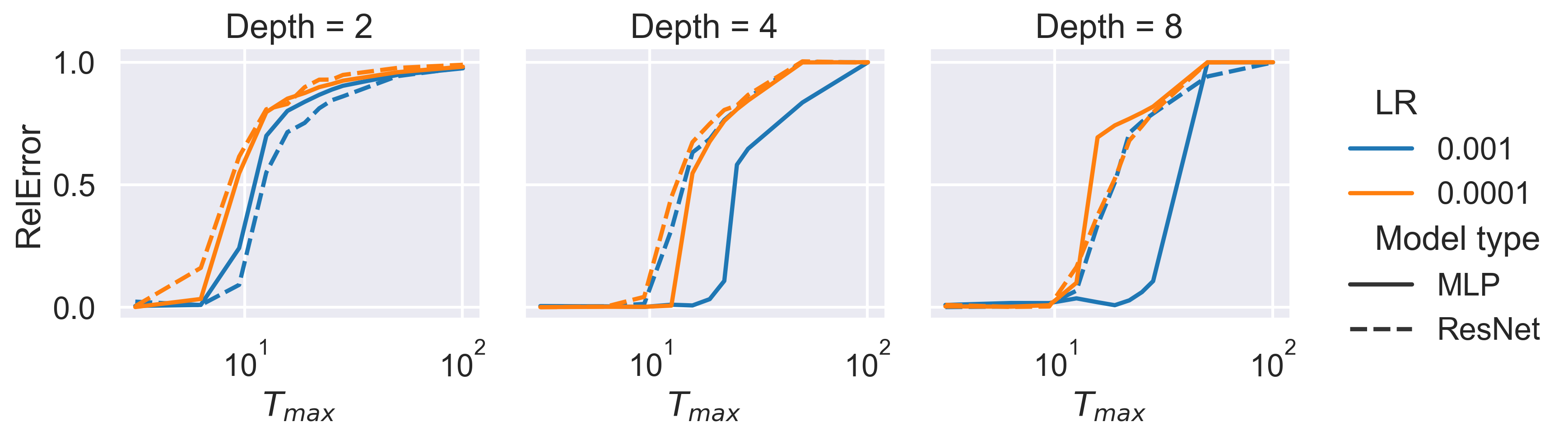
Figure 4: For the SHM benchmark and network depths of 2, 4, and 8, all PINNs increasingly fail to solve the problem as the maximum time $T$ increases. Depth reduces relative error, although error is still dependent on other hyperparameters—the high learning rate of 0.001 and a MLP perform the best. Here we show error results for models under the adaptive weighting PINN formulation with a width of 64 units; results for other PINN configurations are comparable or worse. Upper bounds on $T$ are of form $T_{max}\pi$ when actually training the PINNs. Precise values of maximum time are given in Table 2 in Appendix B.

3.4 Laplacian analysis

In Figure 6, we analyze the Laplacian $\Delta L_{c}$ of the components of the heat equation loss function. We seek trends in the Laplacian as the number of equations varies; thus, we normalize the Laplacian of the residual by the condition number of the discretized differential operator and the Laplacian of the initial condition error by the number of equations. Even with this normalization, there remains a positive correlation between the number and equations and the Laplacian of the residual—the PINN formulation cannot handle the ill-conditioning of the heat equation benchmark.

In Figure 5, we analyze the Laplacian $\Delta L_{c}$ of the components of the SHM loss function. For ResNet architectures, the Laplacian of the residual loss does increase as the maximum time $T$ also increases; however, this increase is not also found for MLP architectures.

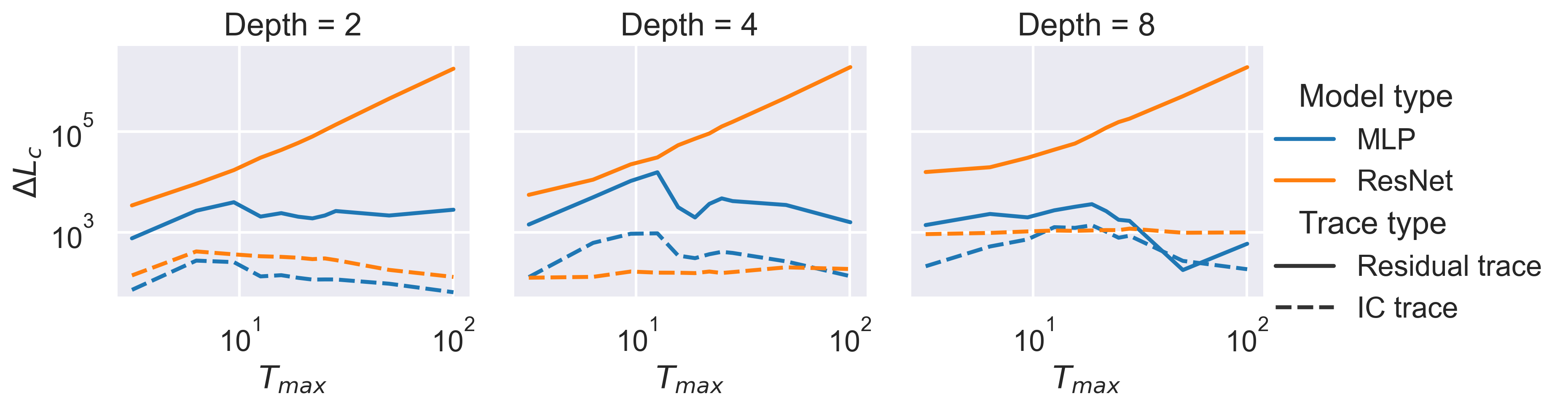
Figure 5: Analysis of the Laplacian $\Delta L_{c}$ of components of the SHM loss function. The Laplacian of the initial condition loss remains fairly constant as network configurations and maximum time $T$ change, reflecting how the initial condition error for this problem is easily satisfied. Interestingly, the Laplacian of PINNs with ResNet networks is consistently much larger than those with MLPs, which aligns with the findings of (Yao et al. 2020) but contradicts findings of (Li et al. 2018); both of whom consider computer vision problems. We show results for the uniform PINN loss formulation, initiated with a learning rate of $10^{-3}$; other results are comparable.

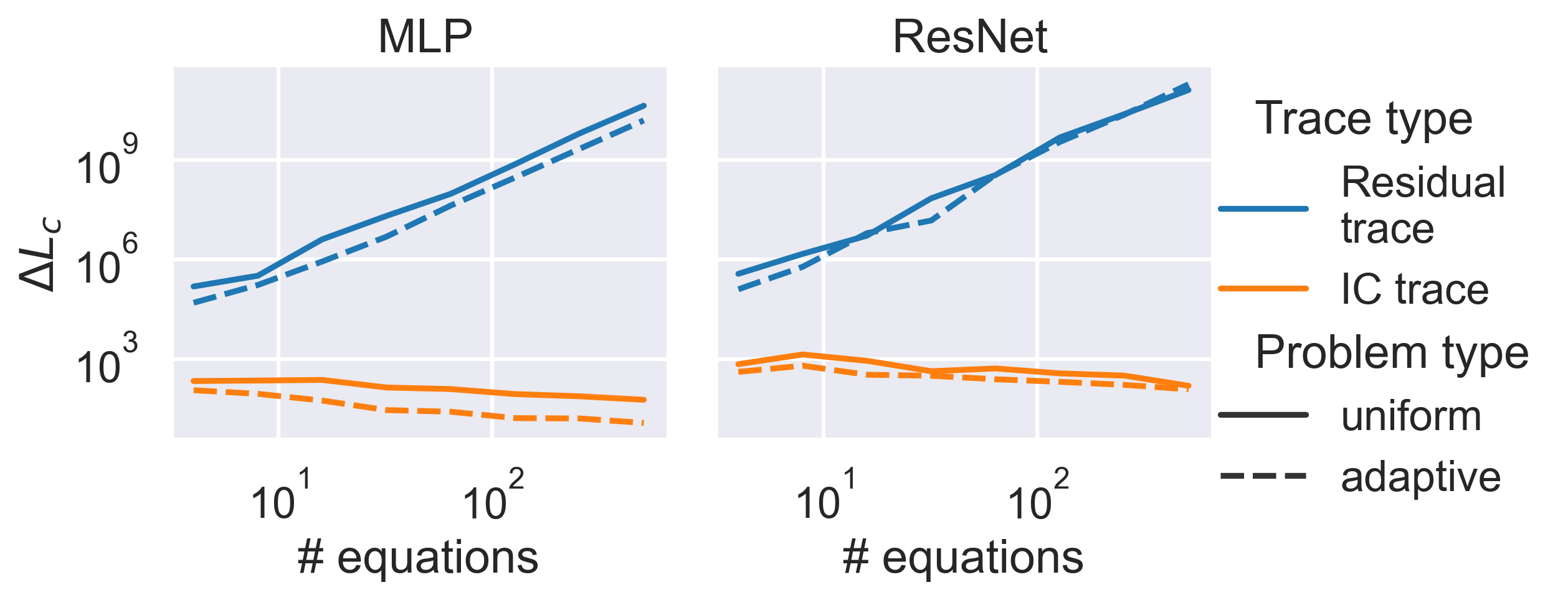
Figure 6: Analysis of the Laplacian $\Delta L_{c}$ of the components of the heat equation loss function, where the residual trace has been normalized by the condition number of the discretized differential operator, and the initial condition trace has been normalized by the number of equations. Under this normalization, the Laplacian of the initial condition loss slightly decreases as the number of equations increases, but the Laplacian of the residual loss increases rapidly. Laplacians of the uniform and adaptive PINN formulations remain comparable, despite the latter performing much worse with respect to relative error (Figure 3). Results are shown for models with 8 hidden layers of 128 units, trained with an initial learning rate of $10^{-3}$.

4 Discussion

In this paper, we demonstrate that, in a pair of benchmarks, the relative error of a PINN falters as problem complexity increases. Our results serve as a cautionary tale in that the ability of modern ML to “reason” in the language of physical laws still remains challenging.

Our experiments can be expanded on in several ways. First, we only consider forward problems, in the assumption that inverse problems would require robust forward prediction capability. This seems necessary, but may not be sufficient for successful solutions to inverse problems. Second, our current results may benefit from a larger sweep of model hyperparameters—which could provide additional insight into PINN behavior and increase confidence in our results. Finally, our choice of two benchmarks is focused on PINN performance for ODEs—as we discuss below, a broader benchmark suite is likely needed.

The two benchmarks chosen for this paper are simple and representative of actual DE modeling problems encountered in scientific applications. We identify Hessian-based metrics as being sometimes representative of a PINN’s ability to solve a problem, but further work remains in a devising a more general classification of PINNs and DEs. This can assist in evaluating novel approaches for PINN architectures, loss functions, and training schemes. Our benchmarks can easily be made more extensive. For example, more than one dimension of complexity can be varied, and a variety of initial conditions can be specified. In addition, similar benchmarks can be developed for PDEs. We believe that a robust suite of benchmarks for physics-informed ML models is needed to facilitate reproducibility and to aid validation of models for difficult problems—such as large, stiff, and multi-scale systems, as well as inverse problems.

Appendix A Details on the heat equation

The continuous-space formulation of the heat equation is:

$$\partial_{t}u = \partial_{xx}u$$

$$u(x,0) = g(x)$$

$$u(0,t) = u_{L}(t)$$

$$u(1,t) = u_{R}(t)$$

$$(x,t) \in (0,1)\times(0,T),$$

where $g$ specifies the initial condition, and $u_{L}$ and $u_{R}$ specify the boundary conditions on the left and right side, respectively, of the spatial domain $(0,1)$. We use an initial condition of $g(x)=\sin(2\pi x)+1$ and boundary conditions of $u_{L}(t)=u_{R}(t)=1$.

The central finite difference approximation to $\partial_{xx}$ is:

$$\partial_{xx}u(x_{n},t)=\frac{u(x_{n+1},t)-2u(x_{n},t)+u(x_{n-1},t)}{(\Delta x)^{2}},$$

which yields the system of linear equations described in Section 2.3.

Appendix B Supplemental tables

Hyperparameter	Value(s) used
# Layers	2, 4, 8
# Hidden units	64, 128
Initial learning rate	$10^{-3},10^{-4}$
Network type	MLP, ResNet
PINN formulation	Uniform, Adaptive
Activation function	$\tanh$
Masking function $\mu$	Sigmoid
# Adam iterations	10,241
# Training points $D$ (SHM)	$256T/\pi$
# Training points $D$ (heat equation)	1,024

Table 1: Hyperparameters searched over when solving PINN problems. For the PINN formulation, Uniform is the standard PINN formulation Equation 1, and Adaptive is the adaptive-weighted PINN formulation Equation 2. The heat equation benchmark uses a fixed number of training points, since their domains do not vary in size; the SHM benchmark scales the number of training points with the time horizon $T$.

Problem	Complexity parameter	Values evaluated	Other parameters
Simple harmonic motion	Maximum time	$T=2^{\ell}\pi,\ell=0,1,\ldots,5$	$N=2$, $\nu_{\mathcal{I}}=1$
Heat equation	# discretized points	$N$ = 4, 8, …, 256, 512	$\nu_{\mathcal{I}}=||\mathbf{A}||_{2},T=0.1$

Table 2: ODE system parameters evaluated. For Section 2.3, since the norm of $\mathbf{A}$ scales with the number of discretizations $N$ and the initial condition remains constant, we scale the initial condition error by $||\mathbf{A}||_{2}$ during training. For Section 2.3, we choose the maximum time $T$ so that the solution has decayed to a constant value.

Appendix C Supplemental Figures

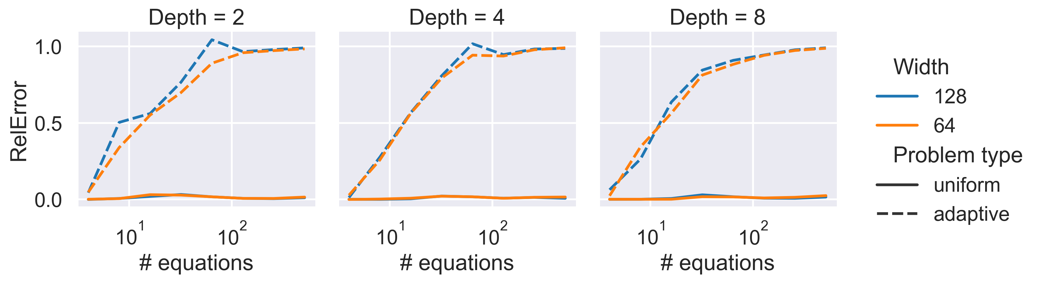
Figure 8: Even though PINNs fail to solve the high-dimensional heat equation over the entire domain, the standard PINN formulation is able to learn the initial condition.

References

- Arthurs and King (2021) Arthurs, C. J.; and King, A. P. 2021. Active Training of Physics-Informed Neural Networks to Aggregate and Interpolate Parametric Solutions to the Navier-Stokes Equations. Journal of Computational Physics, 438: 110364.
- Baydin et al. (2017) Baydin, A. G.; Pearlmutter, B. A.; Radul, A. A.; and Siskind, J. M. 2017. Automatic Differentiation in Machine Learning: A Survey. J. Mach. Learn. Res., 18(1): 5595–5637.
- Brandstetter, Worrall, and Welling (2022) Brandstetter, J.; Worrall, D. E.; and Welling, M. 2022. Message Passing Neural PDE Solvers. In International Conference on Learning Representations.
- Chow, Mallet-Paret, and Van Vleck (1996) Chow, S.-N.; Mallet-Paret, J.; and Van Vleck, E. S. 1996. Dynamics of Lattice Differential Equations. International Journal of Bifurcation and Chaos, 06(09): 1605–1621.
- Daw et al. (2022) Daw, A.; Bu, J.; Wang, S.; Perdikaris, P.; and Karpatne, A. 2022. Mitigating Propagation Failures in PINNs using Evolutionary Sampling. Doi:10.48550/ARXIV.2207.02338.
- Dormand and Prince (1980) Dormand, J.; and Prince, P. 1980. A Family of Embedded Runge-Kutta Formulae. Journal of Computational and Applied Mathematics, 6(1): 19–26.
- He et al. (2016) He, K.; Zhang, X.; Ren, S.; and Sun, J. 2016. Deep Residual Learning for Image Recognition. In 2016 IEEE Conference on Computer Vision and Pattern Recognition (CVPR), 770–778.
- Jacot, Gabriel, and Hongler (2018) Jacot, A.; Gabriel, F.; and Hongler, C. 2018. Neural Tangent Kernel: Convergence and Generalization in Neural Networks. In Advances in Neural Information Processing Systems, volume 31.
- Ji et al. (2021) Ji, W.; Qiu, W.; Shi, Z.; Pan, S.; and Deng, S. 2021. Stiff-PINN: Physics-Informed Neural Network for Stiff Chemical Kinetics. The Journal of Physical Chemistry A, 125(36): 8098–8106.
- Karniadakis et al. (2021) Karniadakis, G. E.; Kevrekidis, I. G.; Lu, L.; Perdikaris, P.; Wang, S.; and Yang, L. 2021. Physics-Informed Machine Learning. Nature Reviews Physics, 3(6): 422–440.
- Kharazmi, Zhang, and Karniadakis (2021) Kharazmi, E.; Zhang, Z.; and Karniadakis, G. E. 2021. hp-VPINNs: Variational Physics-Informed Neural Networks with Domain Decomposition. Computer Methods in Applied Mechanics and Engineering, 374: 113547.
- Kingma and Ba (2014) Kingma, D. P.; and Ba, J. 2014. Adam: A Method for Stochastic Optimization. Doi:10.48550/ARXIV.1412.6980.