The Distribution of Unstable Fixed Points in Chaotic Neural Networks

Abstract

We analytically determine the number and distribution of fixed points in a canonical model of a chaotic neural network. This distribution reveals that fixed points and dynamics are confined to separate shells in phase space. Furthermore, the distribution enables us to determine the eigenvalue spectra of the Jacobian at the fixed points. Despite the radial separation of fixed points and dynamics, we find that nearby fixed points act as partially attracting landmarks for the dynamics.

Chaotic dynamics are well understood in low dimensional systems but are notoriously challenging in high dimensions [1]. In low dimensions, the first step in the analysis of a dynamical system is to determine its fixed points in phase space, for example the two unstable fixed points at the centers of the Lorenz attractor [2]. For high-dimensional nonlinear systems, merely finding all fixed points rapidly becomes prohibitive [3]. Accordingly, the phase space of high-dimensional chaotic systems is still largely terra incognita (see [4] for a recent exception) despite their ubiquitous appearance across disciplines.

Here, we investigate the phase space of a particular high-dimensional nonlinear system: a neural network. Neural networks inherently operate outside equilibrium due to the asymmetric coupling [5, 6] and exhibit chaotic dynamics [7, 8]. Concretely, we consider the canonical model of a chaotic neural network proposed by [7]: $N$ nonlinearly connected units $x_{i}(t)$ receiving a constant external input $\eta_{i}$ and obeying the dynamics

$$\dot{x}_{i} =-x_{i}+\sum_{j=1}^{N}J_{ij}\phi(x_{j})+\eta_{i}$$ (1)

with nonlinear transfer function $\phi(x)=\tanh(x)$, independent and identically distributed (i.i.d.) coupling weights $J_{ij}\sim\mathcal{N}(0,g^{2}/N)$, and i.i.d. external inputs $\eta_{i}\sim\mathcal{N}(0,D)$. Due to the directional nature of synapses, the coupling weights are asymmetric.

A major advantage of the recurrent network model (1) is that the analytical approach of dynamical mean-field theory [7, 9] (pedagogically reviewed in [10]) led to a deep understanding of its dynamics at large $N$. Both without [7, 9] and with [11] external input, the statistics of the activity is well captured by a zero-mean Gaussian process with self-consistent autocorrelation function and the system is chaotic above a critical value of $g=g_{c}$ (without external input $g_{c}=1$). Dynamical mean-field theory has also been successfully applied to various extensions of the model [12, 13, 14, 15, 16, 17, 18, 19, 20, 21, 22, 23]. Furthermore, cross-correlations [24] and the full Lyapunov spectrum have been investigated recently [25]. In summary, the high-dimensional chaotic dynamics of the model are exceptionally well understood.

In contrast to the dynamics, the phase space and the fixed point structure of the model received considerably less attention. The pioneering work [26] showed that for $g=1+\varepsilon$, $0<\varepsilon\ll 1$ and in the absence of external input, the phase space contains a number of fixed points that grows exponentially with the system size $N$. Their finding that the maximum Lyapunov exponent and the rate controlling the exponential increase of fixed points to leading order in $\varepsilon$ coincide led the authors to hypothesize a deep link between the abundance of fixed points and the chaoticity of the dynamics. However, to investigate the relation between the fixed points and the dynamics, a mandatory first step is to establish the location of the fixed points.

In this Letter, we determine the spatial distribution of the fixed points. On the technical level, this requires to compute the expected zero-crossings of a Gaussian process with location dependent, i.e., non-homogeneous, statistics. Afterwards, we compare the geometries of the fixed points and the dynamics to show that both are confined to separate shells in phase space. Next, we leverage the distribution of fixed points to investigate the stability of the local dynamics at the fixed points, from which we deduce that the dynamics closely passes the fixed points. Finally, we argue that the fixed points can be used as landmarks to describe the dynamics symbolically.

Spatial distribution of fixed points.—Throughout the Letter we assume that the network is in the chaotic regime $g>g_{c}$ and that the number of units $N$ is sufficiently large to allow us focus on the leading order behavior, which we express by the abbreviated notation $a\overset{.}{=}e^{Nb}$ to denote $\lim_{N\to\infty}\frac{1}{N}\ln a=b$.

We use vector notation to write Eq. (1) as $\dot{\bm{x}}=\bm{y}(\bm{x})$ with velocity $\bm{y}(\bm{x})=-\bm{x}+\mathbf{J}\phi(\bm{x})+\bm{\eta}$. Since $\mathbf{J}$ and $\bm{\eta}$ are Gaussian, the velocity $\bm{y}(\bm{x})$ and the Jacobian $\bm{y}^{\prime}(\bm{x})=-\mathds{1}+\mathbf{J}\,\mathrm{diag}[\phi^{\prime}(\bm{x})]$ are Gaussian processes (note that both $\bm{y}(\bm{x})$ and $\bm{y}^{\prime}(\bm{x})$ are non-homogeneous). Due to the randomness of $\bm{y}(\bm{x})$, the location of the fixed points $\bm{y}(\bm{x})=0$ is described by a distribution $\rho(\bm{x})$. This distribution counts how many fixed points are on average within an infinitesimal volume in phase space. We determine $\rho(\bm{x})$ from the Kac-Rice formula [27, 28, 29]

$$\rho(\bm{x}) =\left\langle\delta[\bm{y}(\bm{x})]\,\left|\det\bm{y}^{\prime}(\bm{x})\right|\right\rangle_{\mathbf{J},\bm{\eta}}.$$ (2)

The expected number of fixed points $N_{\mathrm{fp}}$ follows from the normalization constant $N_{\mathrm{fp}}=\int_{\mathbb{R}^{N}}d\bm{x}\,\rho(\bm{x})$. The Jacobian determinant $\left|\det\bm{y}^{\prime}(\bm{x})\right|$ in Eq. (2) ensures that every fixed point contributes to the distribution with equal weight. Eq. (2) is equivalent to a random matrix problem: Using Bayes’ law to condition on $\bm{y}(\bm{x})=0$, $\rho(\bm{x})$ can be rewritten into [30, A.1]

$$\rho(\bm{x}) =p_{\mathrm{L}}(\bm{x})\left\langle\left|\det\left[\mathbf{M}(\bm{x})+\mathbf{X}\,\bm{\Sigma}(\bm{x})\right]\right|\right\rangle_{X_{ij}\sim\mathcal{N}(0,N^{-1})}$$ (3)

where the first factor $p_{\mathrm{L}}(\bm{x})=\mathcal{N}(\bm{x}\,|\,0,\kappa(\bm{x})+D)$ with $\kappa(\bm{x})=\frac{g^{2}}{N}\sum_{i=1}^{N}\phi(x_{i})^{2}$ is the probability of the velocity to be zero and the second factor is the expected determinant of a random matrix with mean $\mathbf{M}(\bm{x})$ and covariance $\bm{\Sigma}(\bm{x})^{\mathrm{T}}\bm{\Sigma}(\bm{x})$ controlling for the fluctuations of the velocity process. Here, $\kappa(\bm{x})+D$ is the variance of the Gaussian process $\bm{y}(\bm{x})$ and $\mathbf{M}(\bm{x})$, $\bm{\Sigma}(\bm{x})^{\mathrm{T}}\bm{\Sigma}(\bm{x})$ are the mean and variance, respectively, of the Gaussian process $\bm{y}^{\prime}(\bm{x})$ conditioned on $\bm{y}(\bm{x})=0$. Extending the technique introduced in [31], and excluding singularities, the determinant is given by $\left\langle\left|\det\left[\mathbf{M}(\bm{x})+\mathbf{X}\,\bm{\Sigma}(\bm{x})\right]\right|\right\rangle\overset{.}{=}\exp\big{(}N\zeta(\bm{x})\big{)}$ with [30, A.2]

$$\zeta(\bm{x}) =-\frac{1}{2}z_{*}+\frac{1}{2N}\sum_{i=1}^{N}\ln[1+z_{*}g^{2}\phi^{\prime}(x_{i})^{2}]$$ (4)

where $z_{\ast}$ is the solution of

$$1 =\frac{1}{N}\sum_{i=1}^{N}\frac{g^{2}\phi^{\prime}(x_{i})^{2}}{1+z_{\ast}\,g^{2}\phi^{\prime}(x_{i})^{2}}.$$ (5)

To summarize, the $N$-dimensional distribution of the fixed points is $\rho(\bm{x})\overset{.}{=}\exp\big{(}-NS(\bm{x})\big{)}$ with

$$S(\bm{x}) =\frac{q(\bm{x})}{2[\kappa(\bm{x})+D]}+\frac{1}{2}\ln\left\{2\pi[\kappa(\bm{x})+D]\right\}-\zeta(\bm{x})$$ (6)

where $q(\bm{x})=\frac{1}{N}\sum_{i=1}^{N}x_{i}^{2}$ and $\zeta(\bm{x})$ is determined by Eq. (4) and Eq. (5).

The fixed point distribution Eq. (6) depends on $\bm{x}$ only through network averages. Consequently, it is permutation-symmetric, which implies an approximate independence of coordinates $\int\rho(\bm{x})\,dx_{k+1}...dx_{N}\approx\prod_{i=1}^{k}\mu(x_{i})$ for $k\ll N$ [30, B.3]. Furthermore, we can express it as a functional $\rho(\bm{x})=\rho[\mu_{\bm{x}}]$ of the empirical measure

$$\mu_{\bm{x}}(y) =\frac{1}{N}\sum_{i=1}^{N}\delta(y-x_{i}),$$ (7)

i.e., the empirical distribution of vector components of $\bm{x}$. From the expected empirical measure at the fixed points $\mu_{\ast}(y)=\left\langle\mu_{\bm{x}}(y)\right\rangle_{\bm{x}\sim\rho(\bm{x})}$ all network-averaged expectation values $\left\langle\frac{1}{N}\sum_{i=1}^{N}f(x_{i})\right\rangle_{\bm{x}\sim\rho(\bm{x})}=\int dy\,\mu_{\ast}(y)f(y)$ can be computed. The expected empirical measure is given, for large $N$, by the saddle point that maximizes $\rho[\mu_{\bm{x}}]$ in function space and admits the form [30, B.1]

$$\mu_{\ast}(y)\propto\sqrt{1+\alpha\phi^{\prime}(y)^{2}}e^{-\frac{y^{2}+\gamma\phi(y)^{2}}{2\beta}},$$ (8)

for which the parameters $\alpha$, $\beta$, and $\gamma$ are determined by $1=g^{2}\big{\langle}(\phi^{\prime}(y)^{-2}+\alpha)^{-1}\big{\rangle}_{\mu_{\ast}}$, $\beta=g^{2}\big{\langle}\phi(y)^{2}\big{\rangle}_{\mu_{\ast}}+D$, and $\gamma=g^{2}\big{(}1-\beta^{-1}\big{\langle}y^{2}\big{\rangle}_{\mu_{\ast}}\big{)}$ where expectation values have to be taken self-consistently w.r.t. $\mu_{\ast}$.

We compare the empirical measure Eq. (8) to the distribution of vector components of numerically determined fixed points.

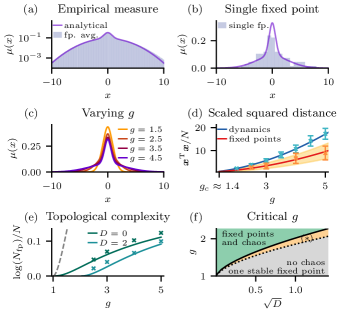
Figure 1: Characterization of fixed points. (a) Distribution of vector components of fixed points (empirical measure): theoretical result (solid line) based on Eq. (8) and histogram (bars) averaged across $4\times 10^{4}$ fixed points for a single realization of the coupling weights. (b) Same as (a) for a randomly chosen single fixed point. (c) Empirical measure for different values of $g$. (d) Scaled squared norm of fixed points (theory: red solid line; theoretical finite-size standard deviation: yellow shading; numerical results: orange error bars) and dynamics (theory: blue solid line; numerical integration averaged over $15$ realizations per $g$: turquoise error bars). (e) Number of fixed points (topological complexity; solid lines: theory, Eq. (10); crosses: numerical results, [30, E]; gray dashed line: theory for $g\rightarrow 1^{+}$, $D=0$ by [26]). (f) Transition to positive topological complexity (black dotted line) and transition to chaos (black solid line) based on [11]. In the regime $(\ast)$ the phase space exhibits an exponential number of fixed points but the dynamics are not chaotic. Parameters: $D=0.1$ for (a)–(d), $g=4$ for (a) and (b), $N=100$ for numerical results and the shading in (d).

For the numerical results, we fix the realization of the random parameters and employ a Levenberg-Marquart rootfinder starting from independent normally distributed initial conditions until saturation, i.e., until almost no new fixed points are found (see [30, E]). We see in Fig. 1(a) that the theory Eq. (8) is in excellent agreement with the empirical measure averaged over all fixed points found numerically in a single realization of $\mathbf{J}$ (see [30, Fig. 2(a)] for further examples). Moreover, as shown in Fig. 1(b), even single fixed points closely resemble the expected empirical measure.

Indeed the probability distribution functional of the empirical measures takes the form $P[\mu]\overset{.}{=}\exp(-NH[\mu])$ with an analytically determined rate functional $H[\mu]$ [30, B.2], i.e., it obeys a large deviation principle [32, 33]. The minimum of $H[\mu]$ is attained at the expected empirical measure $\mu_{\ast}$. Since $P[\mu]$ quantifies both the variability within a realization of the parameters as well as across realizations [30, B.2], akin to the law of total variance, deviations of $\mu$ from $\mu_{\ast}$ are rare for large $N$ even at the level of individual fixed points. Mismatches between $\mu_{\bm{x}}$ and $\mu_{\ast}$ for a fixed point $\bm{x}$ are thus finite size effects (see [30, Fig. 2(b)] for further examples).

Geometry of fixed point distribution.—The excess kurtosis of $\mu_{\ast}$ reflects the compromise between the two contributions in the fixed point density Eq. (3): high probability of a vanishing velocity, captured by $p_{\mathrm{L}}(\bm{x})$, and a steep expected slope to increase the density of zero crossings, captured by the determinant. The former leads to the broad Gaussian base and the latter to the sharp peak. Geometrically the excess kurtosis implies that the fixed points are posed in the vicinity of spans of subsets of axes in phase space.

The expected value of the scaled squared distance $u_{\bm{x}}=\frac{1}{N}\bm{x}^{\mathrm{T}}\bm{x}$, which quantifies the distance to the origin, is $u_{\ast}=\int dy\,y^{2}\mu_{\ast}(y)$. The distribution of the distance $P(u)$ inherits the exponential form of $P[\mu]$ because $u$ is determined by the empirical measure; formally, this is a consequence of the contraction principle [32]. Thus, $P(u)\overset{.}{=}\exp(-NI(u))$ where the rate function is

$$I(u)=\inf_{\mu:\,\int y^{2}\mu(y)\,dy=u}H[\mu].$$ (9)

The rate function is again $\mathcal{O}(1)$; hence, for $N\gg 1$, the fluctuations of the distance vanish and the fixed points are distributed on a thin spherical shell with radius $\sqrt{Nu_{\ast}}$. In Fig. 1(d), we show the average distance and fluctuations based on Eq. (9) (see [30, C.1]) for $N=100$.

To put the fixed point’s distance to the origin into context with the dynamics we leverage the result from dynamic mean-field theory that the network-averaged variance $q[\bm{x}(t)]=\frac{1}{N}\sum_{i=1}^{N}x_{i}(t)^{2}$ is self-averaging for stationary statistics with fluctuations vanishing in the large $N$ limit [10, 22]. Hence, also the trajectory is embedded in a thin shell around the origin, which is of radius $\sqrt{Nq}$.

The confinement to a thin spherical shell is a generic feature of high-dimensional, weakly correlated random variables [34] but the radius depends on the underlying high-dimensional distribution. Thus, we compare the radii of the two shells in Fig. 1(d). For all $g>g_{c}$, the fixed points shell is inside of the trajectories shell. Furthermore, for $N\rightarrow\infty$, the overlap between the shells vanishes and thus the trajectory is clearly separated from the fixed points in phase space.

Number of fixed points.—A core result of [26] is that without noise, $D=0$, the system has a transition from a single stable fixed point to an exponential number of unstable fixed points $N_{\text{fp}}\overset{.}{=}\exp[cN]$ at $g_{c}=1$. The respective rate $c$, the topological complexity, is

$$c=\frac{\gamma-\alpha}{2g^{2}}-D\frac{\gamma}{2\beta g^{2}}+\ln\mathcal{Z}-\frac{1}{2}\ln(2\pi\beta)$$ (10)

where $\mathcal{Z}$ is the normalization of Eq. (8). Asymptotically, at $D=0$, $c\to-\frac{1}{\pi}+\ln\big{[}1+\mathrm{erf}(\sqrt{1/\pi})e^{1/\pi}\big{]}$ for $g\to\infty$ and $c=\big{(}\frac{2}{3}\big{)}^{4}\epsilon^{3}+O(\epsilon^{4})$ for $g-1=\epsilon\to 0$ [30, C.3]. In Fig. 1(e), we see that the critical gain parameter $g_{c}$ grows with $D>0$; the corresponding transition line is shown in Fig. 1(f). For $D\ll 1$, the transition to an exponential number of fixed points coincides with the transition to chaos. For larger noise strengths $D$, however, a regime exists where the system has an exponential number of fixed points yet the dynamics are not chaotic (see [35] for a similar observation). Both our theory and numerical results are in agreement with the critical point $g_{c}=1$ for $D=0$ found by [26] but the quantitative value of the topological complexity differs clearly from the result by [26] and is well-captured by our theory Fig. 1(e).

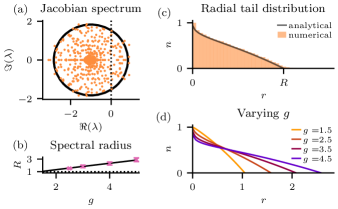
Figure 2: Jacobian spectrum at fixed points. (a) Eigenvalues (orange dots) of the Jacobian at five randomly chosen fixed points of one realization of $\mathbf{J}$ and $\bm{\eta}$. Every eigenvalue with positive real part corresponds to an unstable mode of the fixed point. The support of the spectrum (black circle) is determined by the spectral radius, Eq. (11). (b) Spectral radius; theory (black line) and numerical results (pink errorbars). (c) Radial tail distribution of eigenvalues; theory (black line) based on Eq. (12) and histogram (orange bars) based on the eigenvalues shown in (a). (d) Theory from (c) for varying $g$. Parameters: $N=100$, $g=3$ in (a) and (c), $D=0.1$.

Stability of fixed points.—We now consider the dynamics in the vicinity of fixed points $\bm{x}^{\ast}$. Local stability is determined by the eigenvalues of the Jacobian at the fixed point $\bm{y}^{\prime}(\bm{x}^{\ast})$ (see Fig. 2(a)): Each eigenvalue with positive (negative) real part corresponds to an unstable (stable) eigendirection of the fixed point. The Jacobian can be written as $\bm{y}^{\prime}(\bm{x})=-\mathds{1}+\mathbf{X}\,\mathrm{diag}[g\phi^{\prime}(\bm{x})]$ with $X_{ij}\sim\mathcal{N}(0,N^{-1})$; the corresponding eigenvalue spectrum can be computed with the method developed in [36] because $\mathrm{diag}[g\phi^{\prime}(\bm{x})]$ is invertible. For large $N$, the eigenvalue distribution of $\bm{y}^{\prime}(\bm{x})$ is centered around $-1+0i$ and confined within a circle of radius $R(\bm{x})=g\sqrt{N^{-1}\phi^{\prime}(\bm{x})^{\mathrm{T}}\phi^{\prime}(\bm{x})}$. At a fixed point, the contraction principle attests a large deviation principle for the spectral radius, with the expected value given by

$$R_{\ast}=g\sqrt{\int dy\,\phi^{\prime}(y)^{2}\mu_{\ast}(y)}.$$ (11)

This radius is always $>1$ in the chaotic phase (Fig. 2), indicating that for large $N$ all fixed points are unstable.

Within the support the distribution of eigenvalues is isotropic around the center. We express the distribution by the fraction of eigenvalues further than $r$ from the center $n_{\bm{x}}(r)$, i.e., the radial tail distribution. It obeys, again, a large deviation principle dominated by the solution $n_{\ast}(r)$ of

$$1=\int dy\,\mu_{\ast}(y)\frac{g^{2}\phi^{\prime}(y)^{2}}{r^{2}+n_{\ast}(r)\,g^{2}\phi^{\prime}(y)^{2}}.$$ (12)

We present the solution in Fig. 2(c). The unstable modes of fixed points are underrepresented relative to a uniform spectrum. The overrepresentation of eigenvalues on the real line [Fig. 2(a)] and the smearing of the spectral radius [Fig. 2(c)] are known finite size effects [37, 38].

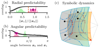
Figure 3: Impact of fixed points. (a) Pearson correlation between $\bm{y}(\bm{x}_{0})$, where $\bm{x}_{0}$ is on the attractor, and its linear predictor $\bm{y}(\bm{x}_{1})+\bm{y}^{\prime}(\bm{x}_{1})[\bm{x}_{0}-\bm{x}_{1}]$ for radially perturbed points $\bm{x}_{1}$ (black line), and nearest fixed points (purple errorbar). Density of norm of the fixed points that are closest to the dynamics (pink) and to random points (green) and mean norm of all fixed points (dashed line). Parameters: $g=5$, $D=0$, and $N=300$ (perturbations), and $N=100$ (fixed points), shadings denote standard deviation. (b) Like (a) but for angular perturbed points $\bm{x}_{1}=a\bm{x}_{0}+\sqrt{1-a^{2}}\|\bm{x}_{0}\|\bm{z}$, where $z_{i}\overset{\mathrm{i.i.d.}}{\sim}\mathcal{N}(0,1/N)$. (c) Sketch of trajectories (blue lines) meandering around the projections (black stars) onto the dynamics shell of some fixed points (red stars), and the resulting symbolic dynamics (red arrows).

Impact of fixed points.—In [26], it is conjectured that the dynamics meanders around the different fixed points, first following their stable directions and then being repelled along their unstable directions. The radial separation of fixed points and dynamics seemingly contradicts this hypothesis.

The conjecture assumes that linearizing the velocity at the nearest fixed point $\bm{x}^{\ast}$ provides a satisfactory prediction of the actual velocity $\bm{y}[\bm{x}(t)]$. Given the linear predictor $\bm{y}_{1}\equiv\bm{y}(\bm{x}^{\ast})+\bm{y}^{\prime}(\bm{x}^{\ast})\left[\bm{x}(t)-\bm{x}^{\ast}\right]$ we quantify the accuracy of the prediction by the time-averaged Pearson correlation between $\bm{y}[\bm{x}(t)]$ and $\bm{y}_{1}$. Points that are radially shrunk or stretched still predict the dynamics well [Fig. 3(a)] whereas points that are rotated by a fixed angle into a random tangential direction quickly decline in predictive power [Fig. 3(b)]. On average, the correlation with the nearest fixed points’ linear predictor is approximately $0.5$ (purple error bar) which corroborates the intuitive picture by [26]. The remaining gap to perfect predictability must be predominantly attributed to the angular, instead of the radial, separation (pink histograms) although the angular separation is small compared to the angular separation between fixed points and random control points that are statistically equivalent to the dynamics (green histograms).

The small angular distance at which the dynamics passes the fixed points results from a majority of attractive directions: In [30, D.1] we show that almost every sample from a sphere around a fixed point moves towards it. In contrast, the expected constant velocity of equivalent points $\bm{p}$, $p_{i}\overset{\text{i.i.d.}}{\sim}\mu_{\ast}$, is non-zero which renders $\bm{p}$ highly repulsive. In this sense, fixed points can be seen as landmarks of the dynamics [39]: The dynamics float above the shell of fixed points, visiting the fixed points in a chain that symbolically describes the dynamics [Fig. 3(c)].

Discussion.—In this Letter we characterize the phase space structure of a chaotic neural network using the distribution of fixed points. We identify a decoupling of the chaos transition and the emergence of unstable fixed points. We furthermore show a spatial separation between fixed points and dynamics. Last, we establish the dynamic role of the fixed points as attractive landmarks for the trajectory.

In high-dimensional linear dynamical systems, May’s pioneering stability analysis [40] enabled considerable insights into the dynamics of ecosystems [41]. In the nonlinear case, the number of fixed points can be determined if the velocity is generated by a homogeneous Gaussian potential [42]; in this case, it is even possible to determine the number of minima of the potential [43, 44, 45] with applications in deep learning [46, 47]. The non-potential case has been addressed in [26] for the random network (1) at $g=1+\varepsilon$ with $\varepsilon\ll 1$, in [48] for a velocity field based on a homogeneous Gaussian field (for which it is possible to extend the analysis to the fraction of stable directions of fixed points [49]), and in [4, 50] for a Lotka-Volterra model. Other non-homogeneous cases have been studied in [51] with dynamics constrained to a sphere and in [52] with a metastable model where the distance of the fixed points to the origin determines which initial conditions decay or escape. For a recent review on stationary points of random fields see [53]. Here, we go beyond the previous results and determine distribution of fixed points, which includes their number, of the random neural network (1) for arbitrary $g>g_{c}$. To this end, we extend methods from random matrix theory [31, 36] to compute the determinant of non-hermitian random matrices with a correlation structure including low-rank terms. The analysis is restricted to the average number of fixed points, which provides an upper bound to the typical number of fixed points [4, 50]. Our numerical results suggest that the bound is rather tight; for the density of fixed points we expect no difference between average and typical behavior, in line with the excellent match of empirical and theoretical density.

The results presented here pave the way towards a mechanistic understanding of the velocity field underlying high dimensional chaotic networks. There are several directions for further research: First, it would be interesting to extend the analysis to more structured networks, e.g., in terms of low rank perturbations [19], levels of symmetry [31, 54, 55], or population structure [15, 14, 22]. Second, the frustration created by the quenched rotation between the axes system, singled out by the element-wise application of the nonlinearity, and the eigensystem of the connectivity creates the complexity of the phase space. What is the geometric relation between the axes system and the dynamics on the chaotic attractor? Last, deep insights into trained neural networks are possible by analyzing their phase space [56, 57]. Here, we analyzed the phase space of a random reservoir which already allows universal computation if the readout is optimized [58]—more generally, learning with chaotic networks [59, 21, 60] is a direction of research that might be able to leverage the exponential number of fixed points and the associated capability for sequence processing.