Compensating for non-linear distortions in controlled quantum systems

Abstract

Predictive design and optimization methods for controlled quantum systems depend on the accuracy of the system model. Any distortion of the input fields in an experimental platform alters the model accuracy and eventually disturbs the predicted dynamics. These distortions can be non-linear with a strong frequency dependence so that the field interacting with the microscopic quantum system has limited resemblance to the input signal. We present an effective method for estimating these distortions which is suitable for non-linear transfer functions of arbitrary lengths and magnitudes provided the available training data has enough spectral components. Using a quadratic estimation, we have successfully tested our approach for a numerical example of a single Rydberg atom system. The transfer function estimated from the presented method is incorporated into an open-loop control optimization algorithm allowing for high-fidelity operations in quantum experiments.

I Introduction

Over the last few decades, various quantum systems, including superconducting circuits, neutral atoms, trapped ions, and spins [1, 2, 3], have shown exciting progress in controlling quantum effects for applications in quantum sensors [4], simulators [5], and computers [6]. In these setups, quantum operations are implemented using external fields or pulses which are generated and influenced by several electronic and optical devices. For high-fidelity and uptime applications, this requires high performance of, e.g., population transfers and quantum gates, while suppressing interactions with the environment as well as decoherence. By shaping temporal and spatial profiles of external fields and pulses, the time-dependent system Hamiltonian steers the quantum dynamics towards the targeted outcome.

Experimental distortions of the applied pulses may reduce the effectiveness and robustness of the desired quantum operation [7, 8]. Methods have been developed to characterize distortions based on the impulse response or transfer function of the experimental system [9, 7, 10, 11, 12, 13, 14, 8, 15]. These approaches for estimating field distortions work well for distortions with a linear transfer function. This work, however, addresses the more general case with substantial non-linear distortions originating from the experimental hardware.

The description of the distortions can be challenging without knowing the exact characteristics of the experimental hardware. Also, approximating a significant non-linearity using a linear model will result in model coefficients and control pulses that are not robust against experimental distortions and suffer from a loss in fidelity. To account for this problem, we introduce a mathematical model and an estimation method which rely on limited experimental data and can characterize the system behavior up to a non-linearity of finite order. To streamline our presentation, we focus on quadratic non-linearities, but more general non-linearities can be treated similarly. We illustrate our estimation approach with numerical data for a single-Rydberg atom excitation experiment in the presence of significant non-linearities and we highlight how our approach can calibrate for and suppress large distortions. We describe an effective approach for estimating the coefficients of this non-linear model and correct the pulses accordingly. We emphasize that our approach is independent of a specific experimental setup and can therefore be applied to various (spatially or temporally) field-tunable phenomena on different quantum platforms.

Our estimation method for distortions is particularly effective in combination with methods from quantum optimal control [16, 17, 18, 19, 20] and it yields optimized pulses for highly efficient gates while accounting for estimated distortions. To this end, we provide an analytical expression for estimating the Jacobian of the transfer function for quadratic distortions, which can be further generalized to higher orders. We also validate this combined approach with our Rydberg atom excitation example. In the context of quantum control, any inaccuracy in the system Hamiltonian can severely affect the performance of pulses produced by optimal control. Given a reasonably accurate model, control fields might also suffer from discretization effects, electronic distortions, and bandwidth limitations (mostly assumed to be linear). Accounting for these distortions by including the linear transfer function within the dynamics, as well as its combined gradient, has been incorporated in related optimization work [7, 21, 15, 22, 23]. Another strategy for minimizing non-linear pulse distortions is to avoid high frequencies altogether in control pulses [24, 25].

Starting from initial applications [26, 27], optimal control methods have been extensively used in quantum computing, quantum simulation, and quantum information processing [17, 20, 28, 29, 30, 31]. Analytic results applicable to smaller quantum systems shape our understanding for the limits to population transfers and quantum gates (see [17, 20, 32, 33, 34, 35, 36, 37, 38, 39, 40, 41, 42, 43, 44, 45, 46, 47, 48] and references therein). Increasing the efficiency of quantum operations by numerically optimizing and fine-tuning control parameters can rely on open-loop or model-based optimal control methods [49, 50, 51, 52, 7, 53, 54, 55, 56, 57]. Our work on the estimation of distortions can be seen in the context of model-based approaches, which might rely on an accurate gradient calculation of the analytical cost function and thus on the knowledge of the Hamiltonian of the system [17, 7]. This knowledge might be available in naturally occurring qubits (such as atomic, molecular, or optical systems), but may also be estimated in engineered (solid-state) technologies. Similarly, closed-loop (i.e. adaptive feed-forward) control methods [58, 59, 60, 61, 62, 63, 31, 64] are used in situ to reduce adverse experimental effects on the control pulses, while direct (real-time) feedback and reservoir engineering methods can also be used where appropriate to counteract control uncertainties [65, 66].

The paper is organized as follows: Section II sketches the control setup for optimizing quantum experiments and describes the conventional method for estimating the transfer function and its inclusion in the optimization. In Sec. III, we detail our non-linear estimation method using non-linear kernels. We also describe how to derive the transformation matrix and its gradient. The non-linear effects on quantum operations are shown with a numerical example of Rydberg atom excitations in Sec. IV. We apply the estimation methodology to our numerical Rydberg example in Sec. V and discuss requirements on the available measurement data. Finally, we consider different numerical optimization methods in combination with our estimation method in Sec. VI (see also Appendix A) and conclude in Sec. VII. The raw data files from the simulations performed for this work are provided in [67].

II Time-dependent Control Problems

We aim to efficiently transferring the population from an initial quantum state to a final target state. The evolving state of a quantum system is described by its density operator $\rho(t)$ and the corresponding equation of motion is written for coherent dynamics as

$$\dot{\rho}=-i[H(t),\rho]+\mathcal{L}(\rho).$$ (1)

The form of the Lindblad term $\mathcal{L}(\rho)$ is discussed in Sec. IV while the Hamiltonian can be expressed as

$$H(t)=H_{d}+\sum_{i}{u_{i}(t)\,H_{i}}.$$ (2)

The free-evolution or drift component is given by $H_{d}$, while $H_{i}$ denotes the control Hamiltonians which are multiplied with time-dependent control pulses $u_{i}(t)$. More precisely, our goal is to transfer a quantum system from a given initial pure state with density operator $\rho_{i}$ to a target pure-state density operator $\rho_{t}$ in time $T$ by varying the control pulses $u_{i}(t)$ while minimizing the cost function

$$C=1-|\langle\rho_{t}|\rho(T)\rangle|^{2}=1-|\mathrm{Tr}[\rho_{t}^{\dagger}\rho(T)]|^{2},$$ (3)

where $\mathrm{Tr}(M)$ denotes the trace of a matrix $M$. This cost function measures the difference between the target-state density operator $\rho_{t}$ and the final-state density operator $\rho(T)$. In this work, we employ gradient-based optimization methods, which are described and discussed in Section VI and Appendix A.

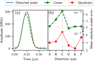
Figure 1: Quadratic estimation of distorted pulses [Eq. (7)] is preferable to linear estimation [Eq. (4)]: (a) A pulse is numerically distorted (solid line); later the distortion is estimated up to linear (dashed line) and quadratic terms (dotted line). The quadratic estimation better matches the actual distorted pulse when compared to the linear estimation. (b) Numerically computed errors for different types of distortions [including the distortion C plotted in (a)] generated by Eqs. (20)–(21) are plotted for both the linear and the quadratic estimation. The error is defined in Eq. (22) and describes the difference between the actual distorted and the estimated pulse.

The experimental realization of control pulses $u_{i}(t)$ relies on several devices, which might introduce systematic distortions and reduce the overall control efficiency. It is our objective to determine these systematic distortions in order to adapt the control pulses during the optimization and counteract any adverse effects. For a linear distortion, we can calculate its transfer function

$$T(\omega)=\frac{Y(\omega)}{X(\omega)}$$ (4)

in the Fourier domain as the ratio of the Fourier transform of the input and output pulses $x(t)$ and $y(t)$, i.e. before and after the distortion has taken place. Alternatively, we can calculate the impulse response $\mathcal{I}(t)$ of the system which relates the input and output pulse in the time domain using the convolution

$$y(t)=(x*\mathcal{I})(t)=\int_{-\infty}^{\infty}x(\tau)\,\mathcal{I}(t{-}\tau)d\tau.$$ (5)

Figure 1 highlights that a linear model might not be sufficient for estimating experimental distortions as it cannot account for non-linear effects. Non-linear effects are demonstrated in Fig. 1(a) by passing one estimated example pulse through a numerically generated distortion [see Eqs. (20)–(21)]. When estimating the distortion coefficients using a linear model, the resulting distorted pulse does not match in Fig. 1(a) with the actual distorted pulse. However, the quadratic estimation with a non-linear model (as described in Sec. III) precisely recovers the actual distorted pulse. Non-linear models are, e.g., preferable for Rydberg excitations which are detailed with realistic experimental parameters in Sec. IV.

III Non-linear Estimation Method

We provide now a general approach for estimating non-linear distortions in a controlled quantum system and explain how this estimation approach can be incorporated into the synthesis of robust optimal control pulses.

III.1 Truncated Volterra series method

We characterize non-linear distortions using the truncated Volterra series method [68]. The Volterra series is a mathematical description of non-linear behaviors for a wide range of systems [69]. In analogy to Eq. (5), we can write the general form of the Volterra series as

$$y(t)=h^{(0)}+\sum_{n=1}^{P}\int_{a}^{b}\!\!\!\ldots\!\int_{a}^{b}h^{(n)}(\tau_{1},\ldots,\tau_{n})\prod_{j=1}^{n}x(t{-}\tau_{j})d\tau_{j}$$ (6)

where $x(t)$ is assumed to be zero for $t<0$ as we consider general, non-periodic signals. The output function $y(t)$ can be expressed as a sum of the higher-order functionals of the input function $x(t)$ weighted by the corresponding Volterra kernels $h^{(n)}$. These kernels can be regarded as higher-order impulse responses of the system. The Volterra series in Eq. (6) is truncated to the order $P<\infty$ and it is called doubly finite if $a$ and $b$ are also finite. For a causal system, the output $y(t)$ can only depend on the input $x(t{-}\tau_{j})$ for earlier times (i.e. $t\geq\tau_{j}$) which results in $a\geq 0$; recall that $x(t{-}\tau_{j})=0$ for $\tau_{j}>t$. The Volterra series can therefore also model memory effects (which are assumed to be of finite length) and it is not restricted to instantaneous effects.

The discretized form of the Volterra series truncated to second order (i.e. $P=2$) is given by ([68, Eq. 2.25])

$$y_{n}=h^{(0)}+\sum_{j=0}^{R-1}h^{(1)}_{j}\,x_{n{-}j}+\sum_{k,\ell=0}^{R-1}h^{(2)}_{k\ell}\,x_{n{-}k}\,x_{n{-}\ell},$$ (7)

The discrete output entries $y_{n}$ have $N$ time steps with $n\in\{0,\ldots,N{-}1\}$ which are obtained from $L$ discrete input entries $x_{q}$ where $x_{q}=0$ for $q<0$. Note that $N=L+R-1\geq L$, where $R\geq 1$ denotes the assumed memory length of the distortion. The memory length $R$ quantifies how the response at the current time step depends on the input of previous time steps, i.e., $R$ bounds the number of previous time steps that can affect the current one. Volterra kernel coefficients of the zeroth, first, and second order are represented by $h^{(0)}$, $h^{(1)}_{j}$, and $h^{(2)}_{k\ell}$. The matrix given by $h^{(2)}_{k\ell}$ is symmetric. We are characterizing the transfer function by estimating the kernel coefficients in Eq. (7). The number $M$ of the to-be-estimated coefficients scales quadratically with the memory length $R$ (in general, the number of coefficients scales with $R^{P}$). Although the Volterra estimation can be extended to any higher order $P>2$, we will focus in this work on the quadratic case.

For the estimation process, we assume that we are provided with a training data set consisting of input-output pulse pairs $(x(t),y(t))$ from an experimental device (or a sequence of devices) which causes the distortion. Next, we discuss how given the training data, we can estimate the kernel coefficients in Eq. (7) by minimizing some error measures (such as the mean square error) between the modeled output and the measured output.

III.2 Truncated Volterra series via least squares

We can choose from different methods to estimate the Volterra series. The most widely used ones are the crosscorrelation method of Lee and Schetzen [70] and the exact orthogonal method of Korenberg [71]. We choose the latter due to its simplicity and as it does not require an infinite-length input. We can write Eq. (7) as

$$y_{n} =\sum_{m=0}^{M-1}u_{nm}\,k_{m}$$ (8)

or equivalently as the matrix equation $$Y=UK$$ or

$$\begin{bmatrix}y_{0}\\ y_{1}\\[-2.84526pt] \vdots\\ y_{N-1}\end{bmatrix} =\begin{bmatrix}u_{00}&u_{01}&\cdots&u_{0,M-1}\\ u_{10}&u_{11}&\cdots&u_{1,M-1}\\[-2.84526pt] \vdots&\vdots&&\vdots\\ u_{N-1,0}&u_{N-1,1}&\cdots&u_{N-1,M-1}\\ \end{bmatrix}\begin{bmatrix}k_{0}\\ k_{1}\\[-2.84526pt] \vdots\\ k_{M-1}\end{bmatrix},$$ (9)

where $K$ is defined in Eq. (11) below. We follow the convention that the entries of a given matrix (or vector) $D$ are represented by $d_{ij}$ (or $d_{i}$). Here, $n\in\{0,\ldots,N{-}1\}$ and $m\in\{0,\ldots,M{-}1\}$ where

$$M=1{+}R{+}R(R{+}1)/2$$ (10)

denotes the number of coefficients that need to be estimated to describe the quadratic Volterra series. In particular, $u_{nm}$ are obtained from the input pulses via (recall again $x_{q}=0$ for $q<0$)

$$u_{nm}=\begin{cases}1&\text{for }\;m=0,\\ x_{n{-}m{+}1}&\text{for }\;m\in\{1,\ldots,R\},\\ {x_{n{-}a}\,x_{n{-}b}}&\text{for }\;m\in\{R{+}1,\ldots,M{-}1\},\end{cases}$$

where $(a,b)$ with $0\leq a\leq b\leq R{-}1$ is the $(m{-}R{-}1)$th element in the lexicographically ordered sequence from $(0,0)$ to $(R{-}1,R{-}1)$. As the quadratic distortion coefficients $h^{(2)}_{k\ell}$ are symmetric, only the upper (or lower) triangular entries need to be considered. The column vector

$$K=[h^{(0)},h^{(1)}_{0},\ldots,h^{(1)}_{R-1},h^{(2)}_{00},\ldots,h^{(2)}_{R-1,R-1}]^{T}$$ (11)

consists of all the Volterra kernels, where $k_{m}=h^{(2)}_{ab}$ for $R{+}1\leq m\leq M{-}1$ and $(a,b)$ is chosen as above.

The example of $R=2$, $L=3$, $N=L+R-1=4$, and $M=6$ results in (with $x_{q}=0$ for $q<0$)

$$\begin{bmatrix}y_{0}\\ y_{1}\\ y_{2}\\ y_{3}\end{bmatrix} =\begin{bmatrix}1&x_{0}&x_{-1}&x_{0}x_{0}&x_{0}x_{-1}&x_{-1}x_{-1}\\ 1&x_{1}&x_{0}&x_{1}x_{1}&x_{1}x_{0}&x_{0}x_{0}\\ 1&x_{2}&x_{1}&x_{2}x_{2}&x_{2}x_{1}&x_{1}x_{1}\\ 1&x_{3}&x_{2}&x_{3}x_{3}&x_{3}x_{2}&x_{2}x_{2}\\ \end{bmatrix}\begin{bmatrix}h^{(0)}\\ h^{(1)}_{0}\\ h^{(1)}_{1}\\ h^{(2)}_{00}\\ h^{(2)}_{01}\\ h^{(2)}_{11}\end{bmatrix}.$$ (12)

For the estimation of the distortions, we need to determine the values of $K$ by solving the matrix equation (9) with the method of least squares. We assume now that the output data vector $Y$ has been measured in an experimental setup. We can also concatenate multiple output pulses into a single vector to form $Y$, which allows us to perform the estimation using multiple short pulses with different characteristics as compared to a single long pulse. This provides the freedom of choosing the format for our training data while observing experimental constraints. In addition to taking a single long pulse or a set of short pulses, we can also repeatedly use the same set of pulses to reduce the measurement error.

As the matrix $U$ contains higher-order terms of the input $x_{n}$, different columns of $U$ are highly correlated with each other. This leads to the problem of solving a linear regression model with a correlated basis set, i.e., the input variables are dependent on each other. The precision of the estimation is adversely affected and less robust when naively applying the method of least squares to solve the matrix equation (9). We resolve this problem by first orthogonalizing the columns of the matrix $U$. The orthogonalization transforms the input variables (stacked in columns of $U$) such that they are independent of each other. After orthogonalizing $U$ to $V$, Eq. (9) is transformed to

$$Y=VW.$$ (13)

Now we can solve the modified matrix equation (13) using the method of least squares to robustly obtain the values of the vector $W$. Finally, if the Gram-Schmidt method is used for orthogonalization, then one can convert $W$ to $K$ by recursive methods (as explained in [71]) to extract the Volterra kernels $h^{(0)}$, $h^{(1)}_{j}$, and $h^{(2)}_{k\ell}$. In this work, we use the QR factorization method which directly provides the values for $K$ [72, 73].

III.3 Gradient of the input response function

Assuming that we have successfully estimated the transfer function, we want to include this information in our gradient-based optimization. This would allow us to also go beyond the piecewise-constant control basis of GRAPE by including arbitrarily deformed controls, generalizing further along the lines of Ref. [7]. We provide now an analytic expression for the corresponding gradient (i.e. Jacobian) to build upon the earlier work discussed in Appendix A.

We apply the commutativity of the convolution (i.e. $f*g=g*f$), e.g., by changing the integration variable from $\tau$ to $z=t-\tau$ in Eq. (5). Using a slight generalization, Eq. (7) can be rewritten as

$$y_{n}=h^{(0)}+\sum_{j=0}^{L-1}h^{(1)}_{n{-}j}\,x_{j}+\sum_{k,\ell=0}^{L-1}h^{(2)}_{n{-}k,n{-}\ell}\,x_{k}\,x_{\ell},$$ (14)

where the upper summation bound $L{-}1$ differs from $R{-}1$ in Eq. (7), i.e. integrating over the length of the input instead of the length of the kernel. From Eq. (14), we specify for each time step (indexed by $n$) a scalar $K^{(0)}=h^{(0)}$, a column vector $K^{(1)}_{n}$ with entries $[K^{(1)}_{n}]_{j}=h^{(1)}_{n{-}j}$, and a matrix $K^{(2)}_{n}$ with entries $[K^{(2)}_{n}]_{k\ell}=h^{(2)}_{n{-}k,n{-}\ell}$ for $j,k,\ell\in\{0,\ldots,L{-}1\}$. With this notation, we can write Eq. (14) as a matrix equation

$$y_{n}=K^{(0)}+{X}^{T}K^{(1)}_{n}+{X}^{T}K^{(2)}_{n}{X},$$ (15)

where the column vector $X=(x_{0},\ldots,x_{L-1})^{T}$ has length $L$. The corresponding partial derivatives are given by

$$\frac{\partial{y_{n}}}{\partial{X}}=K^{(1)}_{n}+{X}^{T}[K^{(2)}_{n}+(K^{(2)}_{n})^{T}],$$ (16)

which simplifies for a symmetric quadratic kernel to

$$\frac{\partial{y_{n}}}{\partial{X}}=K^{(1)}_{n}+2{X}^{T}K^{(2)}_{n}$$ (17)

We can calculate $\partial{y_{n}}/\partial{X}$ for all $n$ and then determine the Jacobian. Eventually, the gradient of the cost function (3) is obtained using the chain rule as, e.g., in [7] and as discussed in Appendix A.

IV Non-linear distortions during Rydberg excitations

We illustrate our scenario of non-linear distortions during controlled quantum dynamics with robust state-to-state transfers in a single Rydberg atom experiment. In recent years, Rydberg atoms have been proven to be a promising platform for quantum simulation [74] and quantum computation [75]. One of the most distinctive features of these atoms in quantum experiments is their strong and tunable dipole-dipole interactions [76, 77]. For larger Rydberg atom arrays as for quantum simulators, excitation protocols (and more general operations) from the ground state to the Rydberg state are crucial. We consider a gradient-based optimization of control pulses (without feedback) for tailored excitation pulses as outlined in Sec. II, (see also Sec. VI and Appendix A).

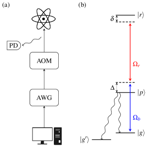
Figure 2: (a) Path of the input control pulse from the computer code via an arbitrary waveform generator (AWG) and an acousto-optic modulator (AOM) to the atom. Before the atom, the output control pulse can be measured using a photodiode (PD). (b) Energy diagram for the excitation of a single Rydberg atom (see text).

The Lindblad master equation for the time evolution of the system is given by Eq. (1). Following [78], the model Hamiltonian for a single Rydberg atom is equal to

$$H(t) =\Omega_{b}(t)\frac{|g\rangle\langle p|+|p\rangle\langle g|}{2}+\Omega_{r}(t)\frac{|p\rangle\langle r|+|r\rangle\langle p|}{2}$$

$$-\Delta|p\rangle\langle p|-\delta|r\rangle\langle r|.$$ (18)

The Rabi frequency $\Omega_{b}(t)$ of the blue laser excites the atom from the ground state $|g\rangle$ to the intermediate state $|p\rangle$ and the Rabi frequency $\Omega_{r}(t)$ excites the atom from $|p\rangle$ to the desired Rydberg state $|r\rangle$ (see Fig. 2(b)). In terms of Eq. (2), $\Omega_{b}(t)$ and $\Omega_{r}(t)$ constitute time-dependent control pulses (such as given by STIRAP [79]). Moreover, $\Delta$ and $\delta$ are the single-photon and the two-photon resonance detuning, which will be for simplicity assumed to be zero ($\Delta=0$ MHz and $\delta=0$ MHz). The Lindblad operator [80] reads as [78]

$${\mathcal{L}(\rho)=\sum\limits_{j\in\{d,g,g^{\prime}\}}(V_{j}\rho V_{j}^{\dagger})-\tfrac{1}{2}(V_{j}^{\dagger}V_{j}\rho+\rho V_{j}^{\dagger}V_{j})}$$ (19)

where $V_{g}=\sqrt{\Gamma_{g}}|g\rangle\langle p|$, $V_{g^{\prime}}=\sqrt{\Gamma_{g^{\prime}}}|g^{\prime}\rangle\langle p|$, and $V_{d}=\sqrt{\Gamma_{d}}|r\rangle\langle r|$ are the Kraus operators. Here, $\Gamma_{g}={\Gamma}/{3}$ and $\Gamma_{g^{\prime}}={2\Gamma}/{3}$ denote the probability for spontaneous emission from $|p\rangle$ to the ground state $|g\rangle$ or to $|g^{\prime}\rangle$ which represents all other ground-state sublevels. Realistic experimental parameters $\Gamma=2\pi\times 1.41$ MHz and $\Gamma_{d}=2\pi\times 0.043$ MHz have been provided by the Browaeys group, where $\Gamma_{d}$ is the Doppler effect. In a real experiment, the gradients of the controls are restricted due to bandwidth limitations. In particular, the controls cannot have derivatives larger than a certain rise speed given by the experimental setup. In our simulations, we take realistic values for the rise times of $0.1\mu s$ and $0.15\mu s$ for the red and blue laser pulses respectively (which translate into rise speeds).

Let us now discuss how systematic distortions can be introduced in this experimental platform during the processing and forwarding of the control signals which finally act on the atom(s). The path of the control signals is sketched in Fig. 2(a). Starting from some computer program, the input pulse (modulated with a fixed carrier frequency) is passed through an arbitrary waveform generator (AWG) to produce the radio-frequency pulse. This pulse is then used as an input for an acousto-optic modulator (AOM) which modulates the intensity of a laser beam. The final laser pulse is then applied to the atom(s) to perform the excitation. The AOM can shape pulses using optical effects such as dispersion [81, 82]. In this experimental setup, one can measure the laser signal before it acts on the atom(s) using a photo diode. In summary, one can choose the input pulse and measure the output pulse; multiple measured input-output pulse pairs serve as training data, which is used to determine systematic distortions.

In our simulation, we excite the Rydberg atom using the system Hamiltonian from Eq. (18) by applying our optimized input control pulses. After that, we introduce quadratic distortions to the control pulses and repeat the simulation. The discrete linear and quadratic distortions are prepared from Gaussian distributions described by

$$h_{1}(t) =\frac{1}{\sigma\sqrt{2\pi}}\exp[{-\tfrac{(t{-}\mu)^{2}}{2{\sigma_{1}}^{2}}}],$$ (20)

$$h_{2}(t_{1},t_{2}) =J\exp[{-\frac{(t_{1}{-}\mu_{1})^{2}+(t_{2}{-}\mu_{2})^{2}}{2{\sigma_{2}}^{2}}}].$$ (21)

The memory length of the discretized dimensionless distortion is $R$. For the distortions A, B, and C, we have chosen $R=50$, standard deviations $\sigma_{1}$ of $1$, $6$, and $11$, and $\sigma_{2}$ of $4.25$, $6.37$, and $8.50$. Similarly, for the distortions D, E, and F, we have varied $R$ between $20$, $40$, and $60$ while fixing $\sigma_{1}=1$ and $\sigma_{2}=4.25$. The amplitude term $J$ has been kept constant at $5\times 10^{-6}$ in all cases. The example distortion C is shown in Figs. 4(a1) and 4(b1). Throughout this work, the zeroth order kernel is set to $h^{0}=0.1$.

We observe optimized controls with a simulated Rydberg excitation error in the range from $0.06$ to $0.008$ for different pulse lengths (see Fig. 3). As expected, longer total durations for the excitation lead to smaller simulated errors. But longer pulse durations might lead to further decoherence effects in the experimental implementation (particularly when combined with additional experimental steps). We, therefore, aim at reducing the length of the pulses (e.g. to a pulse duration around $0.3\mu s$) with reduced excitation errors. In Fig. 3(a), we notice a uniform increase in the error magnitude when we increase the standard deviation of the Gaussian kernels of Eqs. (20)-(21) for the distortions A to C. The distortions result in larger excitation errors for shorter control durations. The case of $0.1\mu s$ is however an exception, where the distorted pulse incidentally has a lower excitation error when compared with the duration of $0.15\mu s$. The standard deviation is kept constant in Fig. 3(b), but we increase the memory length for the distortions D to F which also results in a larger excitation error. Similar to Fig. 3(a), shorter pulses result in higher excitation errors in Fig. 3(b), where the excitation error for the distortion F for the durations $0.15\mu s$ and $0.2\mu s$ are coincidentally equal. The increased excitation errors suggest that optimized control pulses would be susceptible to distortions when applied in the Rydberg atom experiments (and particularly for short pulse lengths). In Sec. V, we present estimation results building on Sec. III for the considered types of distortions.

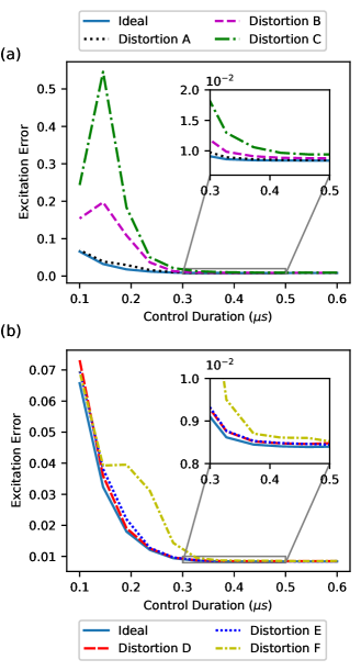
Figure 3: Reduced excitation efficiencies of optimized control pulses due to non-linear distortions in a simulated single Rydberg atom for distortions with (a) an increasing variance but constant memory length (A-C) and (b) a constant variance but increasing memory length (D-F); refer to Sec. IV.

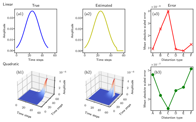
Figure 4: Estimation of both the linear and quadratic components for a non-linear distortion: (a) The linear component (a1) of the distortion C is compared with its estimated value (a2). The amplitude and time steps are dimensionless. (a3) The mean absolute scaled error [as defined in Eq. (22)] between the actual and the estimated values is calculated for various types of distortions A-F [see Eqs. (20)–(21)]. (b) Quadratic component similar as in (a).

V Numerical estimation results

We report in this section on different simulated estimation results which describe the characteristics and precision of applying the Truncated Volterra series method while also comparing multiple types of input control pulses used in the estimation. We also perform the optimization for a single Rydberg excitation again by including the distortions in the algorithm. In each analysis, the estimated results are compared with the actual ones using the mean absolute scaled error (MASE) measure

$$\text{MASE}=\frac{1}{N}\sum_{i=1}^{N}\left|\frac{z^{\text{true}}_{i}}{||z^{\text{true}}||}-\frac{z^{\text{est}}_{i}}{||z^{\text{est}}||}\right|$$ (22)

where $z^{\text{true}}$ is the actual value, $z^{\text{est}}$ is the estimated value, and $||z||$ is the Frobenius norm of the observable $z$ of length $N$. The MASE is numerically more stable compared to the mean relative error, which can be very large when the measured and the actual values are very small.

V.1 Estimation of distortions

We start with the results presented in Fig. 4 where numerical distortions are estimated by relying on a single randomly generated control pulse with $4000$ time steps. We apply different distortions to the pulse and employ the resulting input-output pulse pairs in the estimation. In order to provide a more realistic analysis, we add an additional noise term to the output pulse

$$y_{\text{noise}}=y_{\text{output}}+\tfrac{1}{\sigma\sqrt{2\pi}}\exp[{-\tfrac{(t{-}\mu)^{2}}{2{\sigma}^{2}}}],$$ (23)

where the noise is drawn from a normal distribution with mean $\mu=0$ and standard deviation $\sigma=10^{-4}$. Figures 4(a1)-(b1) display the linear and quadratic contribution of the distortion C. The corresponding estimated contributions are shown in Figs. 4(a2)-(b2) which match closely with values in Figs. 4(a1)-(b1). The results also emphasize that provided we can measure the output pulse accurately, we can calculate the memory length of the distortion (which is here $R=50$) and redundant coefficients are automatically set to zero during the estimation for a sufficiently large $R$ (here set to $60$). The estimation process has been repeated for multiple distortions of type A to F and we observe in Figs. 4(a3)-(b3) low estimation errors of approximately $10^{-7}$ to $10^{-8}$. Slight variations in the estimation error for different distortions could be attributed to the strength of the particular distortion or numerical noise.

We now also compare the estimation method of Sec. III with a linear estimation method in the time domain which relies on a linear impulse response [cf. Eq. (5)]. We omit here the very similar linear estimation in the frequency domain. We again use the distortion types A to F from Sec. IV for this comparison and apply them again to a random-noise pulse of $4000$ steps to obtain input-output pulse pairs for the estimation. Figure 1(a) shows the effect of the true and estimated distortion C when applied to an example pulse of $0.4$$\mu s$ duration. The example pulse is stretched under the distortion to a final duration of $0.65$$\mu s$. The linear estimation is considerably less precise when compared to the quadratic estimation. This effect is confirmed in Figure 1(b) which plots the estimation errors for the different distortion types A-F. Naturally, this also validates that the chosen distortion types contain some non-linearity which is not accounted for by a linear estimation.

V.2 Orthogonalization

One important step of the estimation method is orthogonalization and we have discussed its significance in Sec. III. To further highlight the benefits of orthogonalizing the basis functionals, we test the estimation by directly solving the matrix equation

$${U^{T}Y=U^{T}UK},$$ (24)

where $U$ is the matrix of the non-orthogonalized and correlated basis functionals, $K$ is the to-be-estimated vector of linear or nonlinear kernel coefficients and $Y$ is the measured output vector. We compare the results with coefficients we get from solving the matrix equation (13) with the orthogonalized basis set.

In this analysis, along with the benefit of orthogonalization, we also demonstrate how the estimation depends on the number $M$ of the to-be-estimated coefficients for the distortion, the amount of training data, and the presence of noise in the output pulse. Figures 5(a)-(b) discuss the case without added noise. The nonlinear distortion with $\sigma_{1}=0.1,\sigma_{2}=0.42$ and $R=5$ is estimated using spline input pulses as the training data. Each test and training pulse has 500 time steps and a unique frequency. For a fixed number of spline pulses, we observe in Fig. 5(a) an increasing estimation error for an increasing number of coefficients $M$ (or memory length $R$ as $M\propto{R^{2}}$). For each $M$, we apply the estimation results on $50$ different spline pulses which serve as test data. The corresponding mean error is plotted as a line and the $95\%$ confidence interval is shown as a shaded region around the mean.

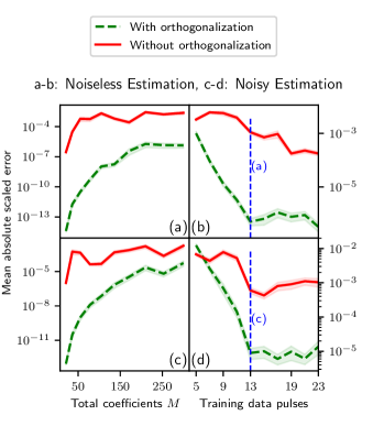
Figure 5: Comparison of the simulated estimation of non-linear distortions without and with orthogonalization solving respectively Eq. (24) and (13): (a) Using a fixed number of noiseless training data for spline input pulses, the relative error rises with an increasing number of coefficients $M$. The plotted line shows the mean error and the shaded area indicates the spread between the $95\%$ confidence interval found from applying the estimation results to $50$ different test pulses. Orthogonalization is advantageous for a larger number of coefficients. (b) Average estimation errors for different training data sets (see text) highlight the importance of increasing the frequency content of the available data. The averaging is performed over the full range of all number of coefficients $M$ in (a). (c)-(d) As in (a)-(b), but the added noise in the output pulses of the data requires a higher frequency content for comparable error rates.

In Fig. 5(b), we gradually increase the number of training pulses used in the estimation. For each fixed number of pulses, we perform the estimation on all the values of $M$ as shown in Fig. 5(a). Hence each point in Fig. 5(b) is averaged over $500$ results. In all cases, the estimation benefits from being performed with orthogonalization. Also, extending the amount of training data points by adding more spline pulses with different frequencies improves the estimation precision as seen in Fig. 5(b). For Figs. 5(c)-(d) in the presence of a noise term in the output pulse with a standard deviation of $10^{-9}$, we observe higher estimation errors which need to be compensated with additional training data points. One can also reduce correlations present in the training data by considering a random input pulse as its autocorrelation is zero. However, even a completely random input pulse results in correlations in $U$ from Eqs. (9) and (24) which contains various non-linear terms of the same input vector [68, p. 165]. In summary, Fig. 5 illustrates the positive effect of orthogonalization on the error rates in the estimation of the distortion.

V.3 Frequency requirements

We investigate different types of training data and their performance in the estimation following the setup of Fig. 6. We can order different training data types according to their increasing frequency content, with Gaussian pulses having the minimum frequency and random-noise pulses having the maximum. Here, the frequency content describes the spectral content of the training data while its value depends on the type of pulses used (see Fig. 5(b) and (d). There are different errors for spline and cosine pulses depending on the amount of data. For a fixed number of pulses, the estimation error grows with an increasing number of coefficients $M$ [see Fig. 6(a)]. Gaussian input pulses are most strongly affected by this, while this effect is essentially negligible in the case of random-noise pulses. This illustrates the importance of spectrally rich input training pulses, which is further emphasized in Fig. 6(b) where the estimation error is plotted, relative to the frequency content. For different types of input pulses, the frequency content is increased differently: we add more pulses with different standard deviations for Gaussian pulses, we add more pulses with different frequencies for cosine pulses, we add more random knots to a single spline. Since a random-noise pulse has a very large bandwidth, we aim at increasing the frequency content by increasing the number of random-noise pulses which only slightly reduces the estimation error. Figure 6(b) highlights that the frequency content is crucial for the estimation and even a single random-noise pulse is highly effective due to its high-frequency content. Splines start to outperform the cosine pulses as soon as they attain higher frequency content than the latter. Similar conclusions hold under noise as shown in Fig. 6(c)-(d) while the overall estimation error increases for the different input pulse types when compared to the noiseless case. The data suggests that a high-frequency content in the training pulses might prevent overfitting noise, which is important when working with real experimental data. Also under noise, random-noise input pulses are most effective in the estimation due to their high frequency content.

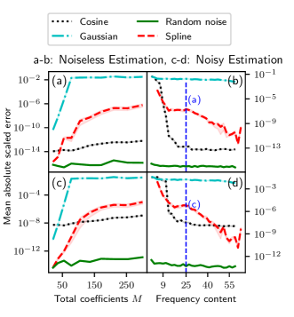
Figure 6: Simulated estimation errors of distortions with multiple types of data: (a) training data with more frequency content (such as random-noise pulses) perform better, even as the number of to-be-estimated coefficients $M$ increases. (b) A lower error can be achieved by increasing the frequency content of the training data. For cosine and Gaussian pulses, the frequency content is increased by adding more pulses with different frequencies, whereas the number of knots is increased within a single pulse for splines. Spectrally rich random-noise pulses are highly effective while keeping the data requirements low. (c)-(d) Similar to (a) and (b), but noisy training data increases the overall error, while random-noise pulses are the most robust. The estimation setup is similar to Fig. 5.

V.4 Compensating for the distortion

With the help of the estimated linear or non-linear distortion coefficients, we compensate for the effect of the distortion on the pulses. One natural approach to find a pre-distorted input pulse shape is to apply the inverted distortion to the target pulse shape. In the case of a linear distortion $T(\omega)$, we would multiply $T^{-1}(\omega)$ with $X(\omega)$ [see Eq. (4)] and later transform it to the time domain. In the non-linear cases and for distortions expressed in time-domain kernels, we solve the following minimization problem to find the pre-distorted pulse

$$\operatorname{argmin}_{x^{\text{input}}}\frac{1}{N}\sum_{i=1}^{N}\left|x^{\text{target}}_{i}{-}\mathcal{D}(x^{\text{input}}_{i})\right|,$$ (25)

where $\mathcal{D}$ applies the distortion. As an example, we correct one analytical Gaussian pulse in order to compensate for the numerical distortion C (see Figure 7). The pre-distorted pulse constructed from the minimization problem produces the ideal Gaussian after passing through the distortion C.

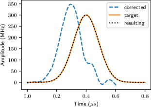
Figure 7: The estimated distortion can be inverted via Eq. (25) and applied to the ideal pulse to produce a pre-distorted pulse. The pre-distorted pulse produces the target Gaussian pulse shape after passing through distortion C.

Next, we perform tests on more complex optimized pulses. As explained in Sec. IV for the single Rydberg excitation, we have two pulses where the blue pulse $\Omega_{b}(t)$ excites the atom from the ground state $|g\rangle$ to the intermediate state $|p\rangle$ and the red pulse $\Omega_{r}(t)$ excites the atom from $|p\rangle$ to the desired Rydberg state $|r\rangle$ [see Fig. 2(b)]. Figure 8 shows pairs of these blue and red pulses as input pulses and the corresponding distorted output pairs. The input pulses in Figure 8(a) are the ideal optimized pulses and when we do not estimate and correct for the distortion, we receive the corresponding output pulses in the experiments.

Next, we estimate the distortion and construct the pre-distorted pulses using the minimization scheme discussed in Eq. (25). The pre-distorted pulses and the corresponding outputs after passing through the distortion are shown in Figure 8(b). Unlike the analytical Gaussian pulse case (see Figure 7), we see that the input pre-distorted pulses do not completely reshape to the ideal optimized pulses after passing through the distortion. This suggests that for more complex pulse shapes, pre-distorting the pulse shape with this method is insufficient to reach a high excitation efficiency. However, we can include the estimated distortion in the optimization to produce pulse shapes that give minimum Rydberg excitation error in the presence of the distortion. The detailed discussion and results of this method are presented in Sec. VI. Figure 8(c) shows an example of input pulses produced from this method and the corresponding distorted output pulses. Note that the input-output pairs in Figure 8(a) and Figure 8(c) are quite similar. We expect this behavior since the excitation error from these example pulses of $0.4\mu s$ duration [see Fig. 9] is not much affected by the distortion. For shorter pulses, the optimization can however produce more complex pulses different from the ideal ones in order to compensate for the distortion. Therefore, we recommend to include the distortion in the optimization to compensate for the effect of the distortion as in Fig. 8(c) and Sec. VI, especially for complex pulse shapes.

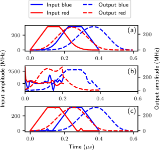
Figure 8: A set of pulses before and after passing through the numerical distortion C in the control chain for the single Rydberg atom excitation. The blue pulse $\Omega_{b}(t)$ excites the atom from the ground state $|g\rangle$ to the intermediate state $|p\rangle$ and the red pulse $\Omega_{r}(t)$ excites the atom from $|p\rangle$ to the desired Rydberg state $|r\rangle$ [see Fig. 2(b)] (a) Optimized input pulses and the corresponding outputs without correction for any distortion. (b) Pre-distorted pulses constructed from the distortion via Eq. (25) and the corresponding output pulses. The output pulses do not match the optimized input pulses from (a). (c) Instead of finding the pre-distorted pulses via Eq. (25), the distortion is included in the optimization to reach the minimum excitation error (see Sec. VI). Pulses from this optimization and the corresponding outputs are shown.

VI Application in optimal control

Starting from early developments in the field, various theoretical and experimental aspects of quantum control have been discussed in the recent review [20]. The overall aim of quantum control is to shape a set of external field pulses that drive a quantum system and perform a given quantum process efficiently. While the analytical way of finding the control parameters works for special cases, one can use highly developed numerical tools in the context of optimal control theory. One solves the Schrödinger or master equation iteratively and produces pulse shapes that perform the desired time evolution. Quantum optimal control is broadly divided into at least the two categories of open-loop and closed-loop. Open-loop methods can be gradient-based or not. Open-loop control is based on the available information about the Hamiltonian of the system and hence it suffers when the system parameters are not completely known such as in the case of an engineered quantum system (such as solid state systems) or when the model cannot be solved precisely as in the case of many-body dynamics [83]. These limitations might be overcome by means of closed-loop optimal control where the control parameters are updated based on the earlier measurements results [61, 62]. Closed-loop quantum optimal control can be implemented via both gradient-based and gradient-free algorithms [84, 85, 86]. In some cases, hybrid approaches have also been suggested [87]. But in the case where the system Hamiltonian is well known, open-loop control provides more freedom to precisely tune the controls depending on experimental constraints and generally explore a wider range of control solutions. Moreover, it also gives a better understanding of the system and works well with systems where fast measurements are not feasible or very noisy, in contrast to closed-loop methods which may require many measurements to converge.

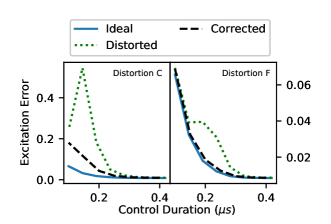
Figure 9: Reduced excitation errors after correcting for the distortion with a gradient-based optimization relying on the trust-region method. (a) distortion C: significant reduced errors, (d) distortion F: mostly recovers the ideal case.

To take full advantage of the open-loop control method and to provide more robust pulses, one can also characterize the experimental system completely or at least partially. Here, we highlight how the estimation method from Sec. III can be employed in an open-loop control setting to minimize the cost function $C$ in Eq. (27) by relying on the corresponding gradients as computed via Eqs. (16) and (30). We refer to Appendix A for details. This compensates for distortions and decreases the error. Figure 9 shows test minimizations of the cost function using the trust-region constrained algorithm [88], which can perform constraint minimization with linear or non-linear constraints on the control pulses. Trust-region methods allow us to explicitly observe bandwidth limitations of the control hardware such as limited rise speeds as discussed in Sec. IV by enforcing the corresponding pulse constraints. Since distortions C and F defined by Eqs. (20) and (21), have the strongest effects on the Rydberg excitation error (see Fig. 3), we correct the control pulses affected by them in the simulations. We limit our test to pulses with shorter durations ranging from 0.1$\mu s$ to 0.4$\mu s$ as they are less susceptible to decoherence and hence might be more suitable for the excitation process. We compare the excitation error produced from the corrected pulse with the ideal and the distorted pulse excitation error. In particular, Figure 9 shows that the effect of the distortion C can be significantly reduced, but it cannot be completely corrected due to a large standard deviation and long memory length in the distortion. The distortion F has a small standard deviation combined with a long memory length which still produces strong effects on the control pulse but with a generally weaker distortion. In this case, the effect of the distortion can be almost completely corrected.

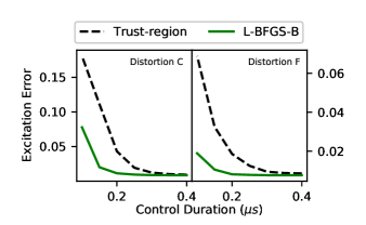
Figure 10: Reduced excitation error for L-BFGS-B when compared to the trust-region method, even though L-BFGS-B does not explicitly enforce constraints on the control pulses (such as limited rise speeds). But the correctly estimated transfer function will implicitly account for pulse constraints. Also, L-BFGS-B is more effective in the optimization.

The estimation of transfer functions in order to correct for distortions has one additional benefit. The experimental hardware given by, e.g., AWGs and AOMs usually has bandwidth limitations which translate into limited rise speeds as discussed in Sec. IV. In the process of characterizing the experimental devices via their transfer function, we also estimate the effects of these bandwidth limitations. The estimated transfer function is then applied during the optimization, which mirrors the effects in the experimental platform and implicitly enforces limitations on the bandwidth or rise time. Assuming that the bandwidth-limiting effect of the estimated transfer function is pronounced enough, this allows us to use the limited memory Broyden–Fletcher–Goldfarb–Shanno (L-BFGS) algorithm to perform the minimization of the cost function [52]. L-BFGS usually offers a more efficient optimization but it cannot explicitly account for general linear or non-linear constraints. In the corresponding optimizations, we only enforce simple box constraints to limit the amplitude of the controls while using the extended L-BFGS or L-BFGS-B algorithm [89]. The results are shown in Fig. 10 where L-BFGS-B improves the excitation efficiency more effectively than the trust-region method (which needs to also explicitly enforce the constraints on the rise speeds). In summary, combining the estimation of distortions with gradient-based optimizations can often effectively compensate for these non-linear distortions during an open-loop optimization.

VII Conclusion

We have proposed a method for estimating non-linear pulse distortions originating from experimental hardware. Hardware limitations affect the performance of optimal control pulses as highlighted using numerical data for single Rydberg atom excitations. In this case, the errors are increased for distorted control pulses beyond purely linear effects. We provide a general model for describing the complex characteristics of these non-linear effects. To incorporate estimated distortions into open-loop optimizations, we have detailed a formula to determine the Jacobian of the transfer function.

We tested and validated our proposed method by efficiently estimating different numerical quadratic distortions with varying strength and duration. We have also shown that linear estimation methods cannot effectively handle non-linear transfer functions. From our detailed analysis and tests, we deduce that the orthogonalization (as described in Sec. V.2) is key for a robust estimation. A robust least-squares estimation is effective only after the orthogonalization is applied to the matrix containing the training data as its correlated columns would otherwise interfere with the estimation. Another critical requirement for effectively performing the estimation is training data with enough frequency content. Large frequency content such as in random-noise pulses better captures the non-linear features of transfer functions, particularly in the presence of measurement noise.

Since the estimation method is independent of any particular type of device characteristics, it can easily be adapted to a wide range of experimental platforms. Combining our estimation method with existing numerical optimization techniques can improve the quality and robustness of quantum operations. Our work thereby addresses a key challenge of enhancing the accuracy and robustness of experimental quantum technology platforms.

Appendix A Optimization algorithm

We work with open-loop optimal control and detail how to incorporate the Jacobian of the transfer function which can be determined following Sec. III.3. In the mathematical statement of an optimal control problem, the fidelity function $C$ is minimized with regard to the control values $u_{i}$. We can apply the gradient-based optimization technique known as GRAPE [49] which can also utilize Newton or quasi-Newton (BFGS) methods [52, 7, 90]. We assume that the total control duration $T$ is divided into $L$ equal steps of duration $\Delta t=T/L$. During each time step, the control amplitudes $u_{i}$ are constant. The time evolution of the quantum system during the $j$th time step is given by

$$U_{j}=\exp{(-i\Delta t(H_{0}+\sum_{i}{u_{i}(j)H_{i}}))}.$$ (26)

The cost function can be written as

$$C=1-|\langle\rho_{t}|{{U_{L}\cdots U_{1}\rho_{i}U_{1}^{{\dagger}}\cdots U_{L}^{{\dagger}}}}\rangle|^{2}.$$ (27)

From the inner product definition and invariance of the trace of a product under cyclic permutations of the factors, Eq. (27) can be rewritten as,

$$1-|\!\underbrace{\langle U_{j+1}^{{\dagger}}\cdots U_{L}^{{\dagger}}\rho_{t}U_{L}\cdots U_{j+1}|}_{\lambda_{j}}\underbrace{{U_{j}\cdots U_{1}\rho_{i}U_{1}^{{\dagger}}\cdots U_{j}^{{\dagger}}}\rangle}_{\rho_{j}}\!|^{2}.$$ (28)

Here, $\rho_{j}$ denotes the density operator at the $j$th time step and $\rho_{t}$ is the backward propagated target operator at the $j$th time step. If we perturb $u_{i}(j)$ to $u_{i}(j)+\delta u_{i}(j)$, the derivative of $C$ is given in terms of the change in $U_{j}$ to the first order in $\delta u_{i}(j)$ which is calculated by the Fréchet derivative method [91] using the Python package SciPy [92].

In order to minimize $C$, at every iteration of the algorithm, we update the controls by

$$u_{i}(j)\rightarrow u_{i}(j)-\epsilon\frac{\delta C}{\delta u_{i}(j)},$$ (29)

where $\epsilon$ is a small unitless step matrix. Next, we follow the derivation in [7], where the product rule for gradient calculation is applied and one obtains

$$\frac{\delta C}{\delta u_{i}(j)}=\sum_{n=0}^{N-1}{\frac{\delta s_{k}(n)}{\delta u_{k}{(j)}}\frac{\delta C}{\delta s_{k}(n)}}\;\text{ where }\;\frac{\delta s_{k}(n)}{\delta u_{k}{(j)}}=T_{k}(n,j).$$ (30)

Compared to (16), $u_{k}$ corresponds to the input pulse $x$ and $s_{n}$ corresponds to the output pulse $y$. Hence we can calculate each column of $T_{k}$ from Eq. (16) as

$$T_{k}(n)=\frac{\delta y_{n}}{\delta X},$$ (31)

and insert $T_{k}$ into Eq. (30) to calculate the effective gradient.

References

- Clarke and Wilhelm [2008] J. Clarke and F. K. Wilhelm, Superconducting quantum bits, Nature 453, 1031 (2008).
- Häffner et al. [2008] H. Häffner, C. Roos, and R. Blatt, Quantum computing with trapped ions, Phys. Rep. 469, 155 (2008).
- Greiner et al. [2002] M. Greiner, O. Mandel, T. Esslinger, T. W. Hänsch, and I. Bloch, Quantum phase transition from a superfluid to a Mott insulator in a gas of ultracold atoms, Nature 415, 39 (2002).
- Gross et al. [2010] C. Gross, T. Zibold, E. Nicklas, J. Estève, and M. K. Oberthaler, Nonlinear atom interferometer surpasses classical precision limit, Nature 464, 1165 (2010).
- Bloch et al. [2012] I. Bloch, J. Dalibard, and S. Nascimbène, Quantum simulations with ultracold quantum gases, Nat. Phys. 8, 267 (2012).
- Kielpinski et al. [2002] D. Kielpinski, C. Monroe, and D. J. Wineland, Architecture for a large-scale ion-trap quantum computer, Nature 417, 709 (2002).
- Motzoi et al. [2011] F. Motzoi, J. M. Gambetta, S. T. Merkel, and F. K. Wilhelm, Optimal control methods for rapidly time-varying Hamiltonians, Phys. Rev. A 84, 022307 (2011).
- Feng et al. [2016] G. Feng, J. J. Wallman, B. Buonacorsi, F. H. Cho, D. K. Park, T. Xin, D. Lu, J. Baugh, and R. Laflamme, Estimating the coherence of noise in quantum control of a solid-state qubit, Phys. Rev. Lett. 117, 260501 (2016).
- Skinner and Gershenzon [2010] T. E. Skinner and N. I. Gershenzon, Optimal control design of pulse shapes as analytic functions, J. Magn. Reson. 204, 248 (2010).
- Gustavsson et al. [2013] S. Gustavsson, O. Zwier, J. Bylander, F. Yan, F. Yoshihara, Y. Nakamura, T. P. Orlando, and W. D. Oliver, Improving Quantum Gate Fidelities by Using a Qubit to Measure Microwave Pulse Distortions, Phys. Rev. Lett. 110, 040502 (2013).
- Spindler et al. [2012] P. E. Spindler, Y. Zhang, B. Endeward, N. Gershernzon, T. E. Skinner, S. J. Glaser, and T. F. Prisner, Shaped optimal control pulses for increased excitation bandwidth in EPR, J. Magn. Reson. 218, 49 (2012).
- Kaufmann et al. [2013] T. Kaufmann, T. J. Keller, J. M. Franck, R. P. Barnes, S. J. Glaser, J. M. Martinis, and S. Han, DAC-board based X-band EPR spectrometer with arbitrary waveform control, J. Magn. Reson. 235, 95 (2013).
- Spindler et al. [2017] P. E. Spindler, P. Schöps, W. Kallies, S. J. Glaser, and T. F. Prisner, Perspectives of shaped pulses for EPR spectroscopy, J. Magn. Reson. 280, 30 (2017).
- Rife and Vanderkooy [1989] D. D. Rife and J. Vanderkooy, Transfer-function measurement with maximum-length sequences, AES: J. Audio Eng. Soc. 37, 419 (1989).
- Le et al. [2022] I. N. M. Le, J. D. Teske, T. Hangleiter, P. Cerfontaine, and H. Bluhm, Analytic filter-function derivatives for quantum optimal control, Phys. Rev. Applied 17, 024006 (2022).
- Brif et al. [2010] C. Brif, R. Chakrabarti, and H. Rabitz, Control of quantum phenomena: past, present and future, New J. Phys. 12, 075008 (2010).
- Glaser et al. [2015] S. J. Glaser, U. Boscain, T. Calarco, C. P. Koch, W. Köckenberger, R. Kosloff, I. Kuprov, B. Luy, S. Schirmer, T. Schulte-Herbrüggen, D. Sugny, and F. K. Wilhelm, Training Schrödinger’s cat: quantum optimal control, Eur. Phys. J. D 69, 279 (2015).
- Schulte-Herbrüggen et al. [2019] T. Schulte-Herbrüggen, R. Zeier, M. Keyl, and G. Dirr, A Brief on Quantum Systems Theory and Control Engineering, in Quantum Information: From Foundations to Quantum Technology Applications, Vol. 2, edited by D. Bruss and G. Leuchs (Wiley, Weinheim, 2019) 2nd ed., pp. 607–641.
- D’Alessandro [2021] D. D’Alessandro, Introduction to Quantum Control and Dynamics, 2nd ed. (CRC Press, Boca Raton, FL, 2021).
- Koch et al. [2022] C. P. Koch, U. Boscain, T. Calarco, G. Dirr, S. Filipp, S. J. Glaser, R. Kosloff, S. Montangero, T. Schulte-Herbrüggen, D. Sugny, and F. K. Wilhelm, Quantum optimal control in quantum technologies. Strategic report on current status, visions and goals for research in Europe, EPJ Quantum Technol. 9, 19 (2022).
- Hincks et al. [2015] I. Hincks, C. Granade, T. W. Borneman, and D. G. Cory, Controlling quantum devices with nonlinear hardware, Phys. Rev. Applied 4, 024012 (2015).
- Jäger and Hohenester [2013] G. Jäger and U. Hohenester, Optimal quantum control of Bose-Einstein condensates in magnetic microtraps: Consideration of filter effects, Phys. Rev. A 88, 035601 (2013).
- Wittler et al. [2021] N. Wittler, F. Roy, K. Pack, M. Werninghaus, A. S. Roy, D. J. Egger, S. Filipp, F. K. Wilhelm, and S. Machnes, Integrated tool set for control, calibration, and characterization of quantum devices applied to superconducting qubits, Phys. Rev. Applied 15, 034080 (2021).
- Sørensen et al. [2020] J. J. Sørensen, J. S. Nyemann, F. Motzoi, J. Sherson, and T. Vosegaard, Optimization of pulses with low bandwidth for improved excitation of multiple-quantum coherences in NMR of quadrupolar nuclei, J. Chem. Phys. 152, 054104 (2020).
- Sørensen et al. [2018] J. J. W. H. Sørensen, M. O. Aranburu, T. Heinzel, and J. F. Sherson, Quantum optimal control in a chopped basis: Applications in control of Bose-Einstein condensates, Phys. Rev. A 98, 022119 (2018).
- Conolly et al. [1986] S. Conolly, D. Nishimura, and A. Macovski, Optimal Control Solutions to the Magnetic Resonance Selective Excitation Problem, IEEE Trans. Med. Imaging 5, 106 (1986).
- Peirce et al. [1988] A. P. Peirce, M. A. Dahleh, and H. Rabitz, Optimal control of quantum-mechanical systems: Existence, numerical approximation, and applications, Phys. Rev. A 37, 4950 (1988).
- Hohenester [2006] U. Hohenester, Optimal quantum gates for semiconductor qubits, Phys. Rev. B 74, 161307 (2006).
- Khani et al. [2009] B. Khani, J. Gambetta, F. Motzoi, and F. K. Wilhelm, Optimal generation of fock states in a weakly nonlinear oscillator, Phys. Scr. 2009, 014021 (2009).
- Goerz et al. [2014] M. H. Goerz, E. J. Halperin, J. M. Aytac, C. P. Koch, and K. B. Whaley, Robustness of high-fidelity Rydberg gates with single-site addressability, Phys. Rev. A 90, 032329 (2014).
- Omran et al. [2019] A. Omran, H. Levine, A. Keesling, G. Semeghini, T. T. Wang, S. Ebadi, H. Bernien, A. S. Zibrov, H. Pichler, S. Choi, J. Cui, M. Rossignolo, P. Rembold, S. Montangero, T. Calarco, M. Endres, M. Greiner, V. Vuletić, and M. D. Lukin, Generation and manipulation of Schrödinger cat states in Rydberg atom arrays, Science 365, 570 (2019).
- Khaneja et al. [2001] N. Khaneja, R. Brockett, and S. J. Glaser, Time Optimal Control in Spin Systems, Phys. Rev. A 63, 032308 (2001).
- Khaneja et al. [2002] N. Khaneja, S. J. Glaser, and R. Brockett, Sub-Riemannian Geometry and Time-Optimal Control of Three-Spin Systems: Quantum Gates and Coherence Transfer, Phys. Rev. A 65, 032301 (2002).
- Bennett et al. [2002] C. H. Bennett, J. I. Cirac, M. S. Leifer, D. W. Leung, N. Linden, S. Popescu, and G. Vidal, Optimal Simulation of Two-Qubit Hamiltonians Using General Local Operations, Phys. Rev. A 66, 012305 (2002).
- Vidal et al. [2002] G. Vidal, K. Hammerer, and J. I. Cirac, Interaction Cost of Nonlocal Gates, Phys. Rev. Lett. 88, 237902 (2002).
- Zeier et al. [2004] R. Zeier, M. Grassl, and T. Beth, Gate Simulation and Lower Bounds on the Simulation Time, Phys. Rev. A 70, 032319 (2004).
- Carlini et al. [2006] A. Carlini, A. Hosoya, T. Koike, and Y. Okudaira, Time-optimal quantum evolution, Phys. Rev. Lett. 96, 060503 (2006).
- Khaneja et al. [2007] N. Khaneja, B. Heitmann, A. Spörl, H. Yuan, T. Schulte-Herbrüggen, and S. J. Glaser, Shortest paths for efficient control of indirectly coupled qubits, Phys. Rev. A 75, 012322 (2007).
- Yuan et al. [2008] H. Yuan, R. Zeier, and N. Khaneja, Elliptic Functions and Efficient Control of Ising Spin Chains with Unequal Couplings, Phys. Rev. A 77, 032340 (2008).
- Zeier et al. [2008] R. Zeier, H. Yuan, and N. Khaneja, Time-optimal synthesis of unitary transformations in a coupled fast and slow qubit system, Phys. Rev. A 77, 032332 (2008).
- Carlini et al. [2011] A. Carlini, A. Hosoya, T. Koike, and Y. Okudaira, Time-optimal CNOT between indirectly coupled qubits in a linear Ising chain, J. Phys. A 44, 145302 (2011).
- Nimbalkar et al. [2012] M. Nimbalkar, R. Zeier, J. L. Neves, S. B. Elavarasi, H. Yuan, N. Khaneja, K. Dorai, and S. J. Glaser, Multiple-spin coherence transfer in linear Ising spin chains and beyond: Numerically optimized pulses and experiments, Phys. Rev. A 85, 012325 (2012).
- Carlini and Koike [2012] A. Carlini and T. Koike, Time-optimal transfer of coherence, Phys. Rev. A 86, 054302 (2012).
- Van Damme et al. [2014] L. Van Damme, R. Zeier, S. J. Glaser, and D. Sugny, Application of the Pontryagin maximum principle to the time-optimal control in a chain of three spins with unequal couplings, Phys. Rev. A 90, 013409 (2014).
- Yuan et al. [2015] H. Yuan, R. Zeier, N. Pomplun, S. J. Glaser, and N. Khaneja, Time-optimal polarization transfer from an electron spin to a nuclear spin, Phys. Rev. A 92, 053414 (2015).
- Freeman [1998] R. Freeman, Spin choreography (Oxford University Press Oxford, 1998).
- Guéry-Odelin et al. [2019] D. Guéry-Odelin, A. Ruschhaupt, A. Kiely, E. Torrontegui, S. Martínez-Garaot, and J. G. Muga, Shortcuts to adiabaticity: Concepts, methods, and applications, Rev. Mod. Phys. 91, 045001 (2019).
- Theis et al. [2018] L. Theis, F. Motzoi, S. Machnes, and F. Wilhelm, Counteracting systems of diabaticities using drag controls: The status after 10 years (a), EPL 123, 60001 (2018).
- Khaneja et al. [2005] N. Khaneja, T. Reiss, C. Kehlet, T. Schulte-Herbrüggen, and S. J. Glaser, Optimal control of coupled spin dynamics: design of nmr pulse sequences by gradient ascent algorithms, J. Magn. Reson. 172, 296 (2005).
- Nigmatullin and Schirmer [2009] R. Nigmatullin and S. G. Schirmer, Implementation of fault-tolerant quantum logic gates via optimal control, New J. Phys. 11, 105032 (2009).
- Tošner et al. [2009] Z. Tošner, T. Vosegaard, C. Kehlet, N. Khaneja, S. J. Glaser, and N. C. Nielsen, Optimal control in NMR spectroscopy: Numerical implementation in SIMPSON, J. Magn. Reson. 197, 120 (2009).
- de Fouquieres et al. [2011] P. de Fouquieres, S. G. Schirmer, S. J. Glaser, and I. Kuprov, Second order gradient ascent pulse engineering, J. Magn. Reson. 212, 412 (2011).
- Machnes et al. [2011] S. Machnes, U. Sander, S. J. Glaser, P. de Fouquières, A. Gruslys, S. Schirmer, and T. Schulte-Herbrüggen, Comparing, optimizing, and benchmarking quantum-control algorithms in a unifying programming framework, Phys. Rev. A 84, 022305 (2011).
- Bergholm et al. [2019] V. Bergholm, W. Wieczorek, T. Schulte-Herbrüggen, and M. Keyl, Optimal control of hybrid optomechanical systems for generating non-classical states of mechanical motion, Quantum Sci. Technol. 4, 190501 (2019).
- Palao and Kosloff [2003] J. P. Palao and R. Kosloff, Optimal control theory for unitary transformations, Phys. Rev. A 68, 062308 (2003).
- Palao and Kosloff [2002] J. P. Palao and R. Kosloff, Quantum Computing by an Optimal Control Algorithm for Unitary Transformations, Phys. Rev. Lett. 89, 188301 (2002).
- Goerz et al. [2019] M. H. Goerz, D. Basilewitsch, F. Gago-Encinas, M. G. Krauss, K. P. Horn, D. M. Reich, and C. P. Koch, Krotov: A Python implementation of Krotov’s method for quantum optimal control, SciPost Phys. 7, 80 (2019).
- Liu et al. [1990] H. Liu, S. J. Glaser, and G. P. Drobny, Development and optimization of multipulse propagators: Applications to homonuclear spin decoupling in solids, J. Chem. Phys. 93, 7543 (1990).
- Goodwin et al. [2018] D. L. Goodwin, W. K. Myers, C. R. Timmel, and I. Kuprov, Feedback control optimisation of ESR experiments, J. Magn. Reson. 297, 9 (2018).
- Bardeen et al. [1997] C. J. Bardeen, V. V. Yakovlev, K. R. Wilson, S. D. Carpenter, P. M. Weber, and W. S. Warren, Feedback quantum control of molecular electronic population transfer, Chem. Phys. Lett. 280, 151 (1997).
- Caneva et al. [2011] T. Caneva, T. Calarco, and S. Montangero, Chopped random-basis quantum optimization, Phys. Rev. A 84, 022326 (2011).
- Doria et al. [2011] P. Doria, T. Calarco, and S. Montangero, Optimal control technique for many-body quantum dynamics, Phys. Rev. Lett. 106, 190501 (2011).
- Rach et al. [2015] N. Rach, M. M. Müller, T. Calarco, and S. Montangero, Dressing the chopped-random-basis optimization: A bandwidth-limited access to the trap-free landscape, Phys. Rev. A 92, 062343 (2015).
- Müller et al. [2022] M. M. Müller, R. S. Said, F. Jelezko, and T. Calarco, One decade of quantum optimal control in the chopped random basis, Rep. Prog. Phys. 85, 076001 (2022).
- Solomon and Schirmer [2011] A. I. Solomon and S. G. Schirmer, Quantum control of two-qubit entanglement dissipation, J. Russ. Laser Res. 32, 502 (2011).
- Motzoi et al. [2016] F. Motzoi, E. Halperin, X. Wang, K. B. Whaley, and S. Schirmer, Backaction-driven, robust, steady-state long-distance qubit entanglement over lossy channels, Phys. Rev. A 94, 032313 (2016).
- Singh et al. [2023] J. Singh, R. Zeier, T. Calarco, and F. Motzoi, Raw data files (2023).
- Mathews and Sicuranza [2000] V. Mathews and G. L. Sicuranza, Polynomial signal processing (Wiley, New York, 2000).
- Cheng et al. [2017] C. Cheng, Z. Peng, W. Zhang, and G. Meng, Volterra-series-based nonlinear system modeling and its engineering applications: A state-of-the-art review, Mech. Syst. Signal Process. 87, 340 (2017).
- Lee and Schetzen [1965] Y. W. Lee and M. Schetzen, Measurement of the Wiener Kernels of a Non-linear System by Cross-correlation, Int. J. Control 2, 237 (1965).
- Korenberg et al. [1988] M. J. Korenberg, S. B. Bruder, and P. J. McLlroy, Exact orthogonal kernel estimation from finite data records: Extending Wiener’s identification of nonlinear systems, Ann. Biomed. Eng. 16, 201 (1988).
- Horn and Johnson [1985] R. A. Horn and C. R. Johnson, Matrix analysis (Cambridge University Press, Cambridge, 1985).
- Golub and Van Loan [1996] G. H. Golub and C. F. Van Loan, Matrix computations, 3rd ed. (The John Hopkins University Press, Baltimore, 1996).
- Weimer et al. [2010] H. Weimer, M. Müller, I. Lesanovsky, P. Zoller, and H. P. Büchler, A Rydberg quantum simulator, Nat. Phys. 6, 382 (2010).
- Saffman et al. [2010] M. Saffman, T. G. Walker, and K. Mølmer, Quantum information with Rydberg atoms, Rev. Mod. Phys. 82, 2313 (2010).
- Jau et al. [2016] Y. Y. Jau, A. M. Hankin, T. Keating, I. H. Deutsch, and G. W. Biedermann, Entangling atomic spins with a Rydberg-dressed spin-flip blockade, Nat. Phys. 12, 71 (2016).
- Browaeys et al. [2016] A. Browaeys, D. Barredo, and T. Lahaye, Experimental investigations of dipole-dipole interactions between a few Rydberg atoms, J. Phys. B 49, 152001 (2016).
- de Léséleuc et al. [2018] S. de Léséleuc, D. Barredo, V. Lienhard, A. Browaeys, and T. Lahaye, Analysis of imperfections in the coherent optical excitation of single atoms to Rydberg states, Phys. Rev. A 97, 053803 (2018).
- Vitanov et al. [2017] N. V. Vitanov, A. A. Rangelov, B. W. Shore, and K. Bergmann, Stimulated raman adiabatic passage in physics, chemistry, and beyond, Rev. Mod. Phys. 89, 015006 (2017).
- Lindblad [1976] G. Lindblad, On the generators of quantum dynamical semigroups, Commun. Math. Phys. 48, 119 (1976).
- Zeng et al. [2007] S. Zeng, K. Bi, S. Xue, Y. Liu, X. Lv, and Q. Luo, Acousto-optic modulator system for femtosecond laser pulses, Rev. Sci. Instrum. 78, 015103 (2007).
- Tzang et al. [2018] O. Tzang, D. Hershkovitz, A. Nagler, and O. Cheshnovsky, Pure sinusoidal photo-modulation using an acousto-optic modulator, Rev. Sci. Instrum. 89, 123102 (2018).
- Castro et al. [2012] A. Castro, J. Werschnik, and E. K. U. Gross, Controlling the dynamics of many-electron systems from first principles: A combination of optimal control and time-dependent density-functional theory, Phys. Rev. Lett. 109, 153603 (2012).
- Li et al. [2017] J. Li, X. Yang, X. Peng, and C.-P. Sun, Hybrid quantum-classical approach to quantum optimal control, Phys. Rev. Lett. 118, 150503 (2017).
- Kelly et al. [2014] J. Kelly, R. Barends, B. Campbell, Y. Chen, Z. Chen, B. Chiaro, A. Dunsworth, A. G. Fowler, I.-C. Hoi, E. Jeffrey, A. Megrant, J. Mutus, C. Neill, P. J. J. O’Malley, C. Quintana, P. Roushan, D. Sank, A. Vainsencher, J. Wenner, T. C. White, A. N. Cleland, and J. M. Martinis, Optimal quantum control using randomized benchmarking, Phys. Rev. Lett. 112, 240504 (2014).
- Rol et al. [2017] M. A. Rol, C. C. Bultink, T. E. O’Brien, S. R. de Jong, L. S. Theis, X. Fu, F. Luthi, R. F. L. Vermeulen, J. C. de Sterke, A. Bruno, D. Deurloo, R. N. Schouten, F. K. Wilhelm, and L. DiCarlo, Restless tuneup of high-fidelity qubit gates, Phys. Rev. Applied 7, 041001 (2017).
- Egger and Wilhelm [2014] D. J. Egger and F. K. Wilhelm, Adaptive hybrid optimal quantum control for imprecisely characterized systems, Phys. Rev. Lett. 112, 240503 (2014).
- Conn et al. [2000] A. R. Conn, N. I. M. Gould, and P. L. Toint, Trust Region Methods (SIAM: Society for Industrial and Applied Mathematics, 2000).
- Byrd et al. [1995] R. Byrd, P. Lu, J. Nocedal, and C. Zhu, A limited memory algorithm for bound constrained optimization, SIAM Journal of Scientific Computing 16, 1190 (1995).
- Dalgaard et al. [2020] M. Dalgaard, F. Motzoi, J. H. M. Jensen, and J. Sherson, Hessian-based optimization of constrained quantum control, Phys. Rev. A 102, 042612 (2020).
- Al-Mohy and Higham [2009] A. H. Al-Mohy and N. J. Higham, Computing the Fréchet Derivative of the Matrix Exponential, with an Application to Condition Number Estimation, SIAM J. Matrix Anal. Appl. 30, 1639 (2009).
- Virtanen et al. [2020] P. Virtanen, R. Gommers, T. E. Oliphant, M. Haberland, T. Reddy, D. Cournapeau, E. Burovski, P. Peterson, W. Weckesser, J. Bright, S. J. van der Walt, M. Brett, J. Wilson, K. J. Millman, N. Mayorov, A. R. J. Nelson, E. Jones, R. Kern, E. Larson, C. J. Carey, İ. Polat, Y. Feng, E. W. Moore, J. VanderPlas, D. Laxalde, J. Perktold, R. Cimrman, I. Henriksen, E. A. Quintero, C. R. Harris, A. M. Archibald, A. H. Ribeiro, F. Pedregosa, P. van Mulbregt, and SciPy 1.0 Contributors, SciPy 1.0: Fundamental Algorithms for Scientific Computing in Python, Nat. Methods 17, 261 (2020).