A polynomial-time approximation scheme for the maximal overlap of two independent Erdős-Rényi graphs

Abstract

For two independent Erdős-Rényi graphs $\mathbf{G}(n,p)$, we study the maximal overlap (i.e., the number of common edges) of these two graphs over all possible vertex correspondence. We present a polynomial-time algorithm which finds a vertex correspondence whose overlap approximates the maximal overlap up to a multiplicative factor that is arbitrarily close to 1. As a by-product, we prove that the maximal overlap is asymptotically $\frac{n}{2\alpha-1}$ for $p=n^{-\alpha}$ with some constant $\alpha\in(1/2,1)$.

1 Introduction

In this paper we study the random optimization problem of maximizing the overlap for two independent Erdős-Rényi graphs over all possible vertex correspondence. More precisely, we fix two vertex sets $V=\{v_{1},\dots,v_{n}\},\mathsf{V}=\{\mathsf{v}_{1},\dots,\mathsf{v}_{n}\}$ with edge sets

$$E_{0}=\{(v_{i},v_{j}):1\leq i<j\leq n\},\ \mathsf{E}_{0}=\{(\mathsf{v}_{i},\mathsf{v}_{j}):1\leq i<j\leq n\}\,.$$ (1.1)

For a parameter $p\in(0,1)$, we consider two Erdős-Rényi random graphs $G=(V,E)$ and $\mathsf{G}=(\mathsf{V},\mathsf{E})$ where $E\subset E_{0}$ and $\mathsf{E}\subset\mathsf{E}_{0}$ are obtained from keeping each edge in $E_{0}$ and $\mathsf{E}_{0}$ (respectively) with probability $p$ independently. For convenience, we abuse the notation and denote by $G$ and $\mathsf{G}$ the adjacency matrices for the two graphs respectively. That is to say, $G_{i,j}=1$ if and only if $(v_{i},v_{j})\in E$ and $\mathsf{G}_{i,j}=1$ if and only if $(\mathsf{v}_{i},\mathsf{v}_{j})=1$ for all $1\leq i<j\leq n$. Let $S_{n}$ be the collection of all permutations on $[n]=\{1,\ldots,n\}$. For $\pi\in S_{n}$, define

$$\mathrm{Overlap}(\pi)\stackrel{{\scriptstyle\text{def}}}{{=}}\sum_{1\leq i<j\leq n}G_{i,j}\mathsf{G}_{\pi(i),\pi(j)}$$ (1.2)

to be the number of edges $(v_{i},v_{j})\in E$ with $(\mathsf{v}_{\pi(i)},\mathsf{v}_{\pi(j)})\in\mathsf{E}$. Our main result is a polynomial-time approximation scheme (PTAS) for this optimization problem.

Theorem 1.1.

Assume $p=n^{-\alpha}$ for some $\alpha\in(1/2,1)$. For any fixed $\varepsilon>0$, there exist a constant $C=C(\varepsilon)$ and an algorithm (see Algorithm 2.3) with running time $O(n^{C})$ which takes $G,\mathsf{G}$ as input and outputs a permutation $\pi^{*}\in S_{n}$, such that

$$\mathbb{P}\left[\frac{\mathrm{Overlap}(\pi^{*})}{n}\geq\frac{1-\varepsilon}{2\alpha-1}\right]=1-o(1),\quad\text{as }n\to\infty.$$ (1.3)

In addition, $\max_{\pi\in S_{n}}\frac{\mathrm{Overlap}(\pi)}{n}$ converges to $\frac{1}{2\alpha-1}$ in probability as $n\to\infty$.

Remark 1.2.

For $\alpha\in(0,1/2)$, a straightforward computation yields that with probability tending to 1 as $n\to\infty$, the overlap is asymptotic to $\frac{n^{2}p^{2}}{2}$ for all $\pi\in S_{n}$. Thus, this regime is trivial if one’s goal is to approximate the maximal overlap in the asymptotic sense. For the “critical” case when $\alpha$ is near $1/2$, the problem seems more delicate and our current method falls short in approximating the maximal overlap asymptotically.

Remark 1.3.

One can find Hamiltonian cycles in both graphs with an efficient algorithm (see [35] as well as references therein) and obviously this leads to an overlap with $n$ edges. Also, a simple first moment computation as in the proof of Proposition 2.1 shows that the maximal overlap is of order $n$. Therefore, the whole challenge in this paper is to nail down the asymptotic constant $1/(2\alpha-1)$.

Remark 1.4.

Theorem 1.1 provides an algorithmic lower bound on the maximal overlap which is sharp asymptotically (i.e., the correct order with the correct leading constant), and we emphasize that prior to our work the asymptotic maximal overlap was not known even from a non-constructive perspective. In fact, the problem of the asymptotic maximal overlap was proposed by Yihong Wu and Jiaming Xu as an intermediate step in analyzing the hardness of matching correlated random graphs, and Yihong Wu and Jiaming Xu have discussed extensively with us on this problem. It is fair to say that we have come up with a fairly convincing roadmap using the second moment method, but the technical obstacles seem at least somewhat daunting such that we did not manage to complete the proof. The current paper was initiated with the original goal of demonstrating an information-computation gap for this random optimization problem (as we have believed back then), but it turned out to evolve in a somewhat unexpected way: not only the maximal overlap can be approximated by a polynomial time algorithm, but also it seems (as of now) this may even be a more tractable approach even if one’s goal is just to derive the asymptotic maximal overlap. Finally, the very stimulating discussions we had with Yihong Wu and Jiaming Xu, while not explicitly used in the current paper, have been hugely inspiring to us. We record this short “story” here as on the one hand it may be somewhat enlightening to the reader, and on the other hand we would like to take this opportunity to thank Yihong Wu and Jiaming Xu in the warmest terms.

1.1 Background and related results

Our motivation is twofold: on the one hand, we wish to accumulate insights for understanding the computational phase transition for matching two correlated random graphs; on the other hand, as mentioned in Remark 1.4 we wished to study the computational transition for the random optimization problem of the maximal overlap, which is a natural and important combinatorial optimization problem known to be NP-hard to solve in the worst-case scenario. We will further elaborate both of these two points in what follows.

Recently, there has been extensive study on the problem of matching the vertex correspondence between two correlated graphs and the closely related problem of detecting the correlation between two graphs. From the applied perspective, some versions of graph matching problems have emerged from various applied fields such as social network analysis [33, 34], computer vision [6, 4], computational biology [39, 42] and natural language processing [21]. From the theoretical perspective, graph matching problems seem to provide another important set of examples with the intriguing information-computation gap. The study of information-computation gaps for high-dimensional statistical problems as well as random optimization problems is currently an active and challenging topic. For instance, there is a huge literature on the problem of recovering communities in stochastic block models (see the monograph [1] for an excellent account on this topic) together with some related progress on the optimization problem of extremal cuts for random graphs [11, 31]; there is also a huge literature on the hidden clique problem and the closely related problem of submatrix detection (see e.g. [43] for a survey and see e.g. [19, 26] and references therein for a more or less up-to-date review). In addition, it is worth mentioning that in the last few decades various framework has been proposed to provide evidence on computational hardness for such problems with random inputs; see surveys [47, 2, 37, 24, 18] and references therein.

As for random graph matching problems, so far most of the theoretical study was carried out for Erdős-Rényi graph models since Erdős-Rényi graph is arguably the most canonical random graph model. Along this line, much progress has been made recently, including information-theoretic analysis [8, 7, 22, 45, 44, 12, 13] and proposals for various efficient algorithms [36, 46, 25, 23, 17, 38, 3, 14, 5, 9, 10, 32, 16, 20, 15, 27, 28]. As of now, it seems fair to say that we are still relatively far away from being able to completely understand the phase transition for computational complexity of graph matching problems—we believe, and we are under the impression that experts on the topic also believe, that graph matching problems do exhibit information-computation gaps. Thus, (as a partial motivation for our study) it is plausible that understanding the computational aspects for maximizing the overlap should shed lights on the computational transition for graph matching problems.

As hinted earlier, it is somewhat unexpected that a polynomial time approximation scheme for the maximal overlap problem exists while the random graph matching problem seems to exhibit an information-computation gap. As a side remark, before finding this approximation algorithm, we have tried to demonstrate the computational hardness near the information threshold via the overlap gap property but computations suggested that this problem does not exhibit the overlap gap property. In addition, we point out that efficient algorithms have been discovered to approximate ground states for some spin glass problems [41, 30], which take advantage of the so-called full replica symmetry breaking property. From what we can tell, [41, 30] seem to be rare natural examples for which approximation algorithms were discovered for random instances whereas the worse-case problems are known to be hard to solve. In a way, our result contributes yet another example of this type and possibly of a different nature since we do not see full replica symmetry breaking in our algorithm.

1.2 An overview of our method

The main contribution of our paper is to propose and analyze the algorithm as in Theorem 1.1. The basic idea for our algorithm is very simple: roughly speaking, we wish to match vertices of two graphs sequentially such that the increment on the number of common edges (within matched vertices) per each matched pair is $(2\alpha-1)^{-1}$.

An obvious issue is that $(2\alpha-1)^{-1}$ may not be an integer. Putting this aside for a moment, we first explain our idea in the simple case when $p=n^{-\frac{3}{4}+\delta}$ with some arbitrarily small $\delta>0$. In this case, our goal is to construct some $\pi\in S_{n}$ such that $\mathrm{Overlap}(\pi)\geq(2-\varepsilon)n$ for an arbitrarily small $\varepsilon>0$. Assume we have already determined $\pi(1),\ldots,\pi(k)$ for some $k\in\left[\frac{\varepsilon}{3}n,\left(1-\frac{\varepsilon}{3}\right)n\right]$ (i.e., assume we have already matched $v_{1},\dots,v_{k}\in V$ to $\mathsf{v}_{\pi(1)},\dots,\mathsf{v}_{\pi(k)}\in\mathsf{V}$). We wish to find some $\ell\in[n]\setminus\{\pi(1),\dots,\pi(k)\}$ such that

$$\sum_{1\leq j\leq k}G_{j,k+1}\mathsf{G}_{\pi(j),\ell}\geq 2\,.$$ (1.4)

Provided that this is feasible, we may set $\pi(k+1)=\ell$. Therefore, the crux is to show that (1.4) is feasible for most of the steps. Ignoring the correlations between different steps for now, we can then regard $\sum_{1\leq j\leq k}G_{j,k+1}\mathsf{G}_{\pi(j),\ell}$ as a Binomial variable $\mathbf{B}(k,p^{2})$ for each $\ell\in[n]\setminus\{\pi(1),\dots,\pi(k)\}$ and thus (1.4) holds with probability of order $(kp^{2})^{2}\gtrsim n^{\delta-1}$. Since there are at least $\varepsilon n$ potential choices for $\ell$, (ignoring the potential correlations for now again) it should hold with overwhelming probability that there exists at least one $\ell$ satisfying (1.4). This completes the heuristics underlying the success of such a simple iterative algorithm.

The main technical contribution of this work is to address the two issues we ignored so far: the integer issue and the correlations between iterations. In order to address the integer issue, it seems necessary to match $\chi$ vertices every step with an increment of $\zeta$ common edges for some suitably chosen $\chi,\zeta$ with $\zeta/\chi\approx(2\alpha-1)^{-1}$. Thus, one might think that a natural analogue of (1.4) shall be the following: there exist $\ell_{1},\ldots,\ell_{\chi}\in[n]\setminus\{\pi(1),\dots,\pi(k)\}$ such that

$$\sum_{1\leq j\leq k}\sum_{1\leq i\leq\chi}G_{j,k+i}\mathsf{G}_{\pi(j),\ell_{i}}\geq\zeta\,.$$ (1.5)

However, (1.5) is not really feasible since in order for (1.5) to hold it is necessary that for some $i\in\{1,\dots,\chi\}$, there exists $\ell\in[n]\setminus\{\pi(1),\dots,\pi(k)\}$ such that $\sum_{1\leq j\leq k}G_{j,k+i}\mathsf{G}_{\pi(j),\ell}\geq\lceil(2\alpha-1)^{-1}\rceil$ (where $\lceil x\rceil$ denotes the minimal integer that is at least $x$). A simple first moment computation suggests that the preceding requirement cannot be satisfied for most steps.

In light of the above discussions, we see that in addition to common edges between the matched vertices and the “new” vertices, it will be important to also take advantage of common edges that are within “new” vertices, which requires to also carefully choose a collection of vertices from $V$ (otherwise typically there will be no edges within a constant number of fixed vertices). In order to implement this, it turns out that we may carefully construct a rooted tree $\mathbf{T}$ with $\chi$ non-leaf vertices and $\zeta$ edges, and we wish that the collection of added common edges per step contains an isomorphic copy of $\mathbf{T}$. To be more precise, let $\operatorname{M}=\{j\in[n]:v_{j}\mbox{ has been matched}\}$ and let $\pi(\operatorname{M})=\{\pi(j):j\in\operatorname{M}\}$, and in addition let $k$ be the minimal integer in $[n]\setminus\operatorname{M}$. We then wish to strengthen (1.5) to the following: there exists $\xi=\zeta+1-\chi$ integers $i_{1},\ldots,i_{\xi}\in\operatorname{M}$, $\chi$ integers $j_{1}=k,j_{2},\ldots,j_{\chi}\in[n]\setminus\operatorname{M}$ and $\chi$ integers $\ell_{1},\ldots,\ell_{\chi}\in[n]\setminus\{\pi(1),\dots,\pi(k)\}$ such that the following hold:

• the subgraph of $G$ induced on $\{v_{i_{1}},\ldots,v_{i_{\xi}}\}\cup\{v_{j_{1}},\ldots,v_{j_{\chi}}\}$ contains $\mathbf{T}$ as a subgraph with leaf vertices $\{v_{i_{1}},\ldots,v_{i_{\xi}}\}$;

• the subgraph of $\mathsf{G}$ induced on $\{\mathsf{v}_{\pi(i_{1})},\ldots,\mathsf{v}_{\pi(i_{\xi})}\}\cup\{\mathsf{v}_{\ell_{1}},\ldots,\mathsf{v}_{\ell_{\chi}}\}$ contains $\mathbf{T}$ as a subgraph with leaf vertices $\{\mathsf{v}_{\pi(i_{1})},\ldots,\mathsf{v}_{\pi(i_{\xi})}\}$.

(In this case, we then set $\pi(j_{i})=\ell_{i}$ for $1\leq i\leq\chi$.) In the above, we require the non-leaf vertices of isomorphic copies of $\mathbf{T}$ to be contained in “new” vertices in order to make sure that the edges we add per each iteration are disjoint. In order for the existence of isomorphic copies of $\mathbf{T}$, we need to pose some carefully chosen balanced conditions on $\mathbf{T}$; see Lemma 2.2, (2.4) and (2.5) below.

Figure 1: A single step in the iterative matching algorithm: the black vertices are matched ones, and the blue vertices are the ones matched in the current step (where a tree is added on both sides with leaves being black vertices).

The existence of $\mathbf{T}$, once appropriate balanced conditions are posed, is not that hard to show in light of [3, 28]. However, the major challenge comes in since we need to yet treat the correlations between different iterative steps. This is indeed fairly delicate and most of the difficult arguments in this paper (see Section 3) are devoted to address this challenge.

Finally, we point out that in order for a high precision approximation of $(2\alpha-1)^{-1}$, we will have to choose integers $\chi,\zeta$ fairly large. Since our algorithm is required to check all $\chi$-tuples over unmatched vertices, we only obtain an algorithm with polynomial running time where the power may grow in the precision of approximation. It remains an interesting question whether a polynomial time algorithm with a fixed power can find a matching that approximates the maximal overlap up to a constant that is arbitrarily close to 1.

2 Proof of Theorem 1.1

2.1 Upper bound of the maximal overlap

In this subsection, we prove the upper bound of Theorem 1.1 in the next proposition.

Proposition 2.1.

For any constant $\rho>\frac{1}{2\alpha-1}$, we have

$$\mathbb{P}\left[\max_{\pi\in S_{n}}\mathrm{Overlap}(\pi)\geq\rho n\right]\to 0\,,\quad\text{as }n\to\infty\,.$$ (2.1)

Proof.

By a union bound we see the left hand side of (2.1) is bounded by

$$\sum_{\pi\in S_{n}}\mathbb{P}\left[\mathrm{Overlap}(\pi)\geq\rho n\right]=n!\mathbb{P}\left[\mathbf{B}\geq\rho n\right],$$

where $\mathbf{B}$ is distributed as a binomial variable $\mathbf{B}(\binom{n}{2},p^{2})$. By standard large deviation estimates for binomial variables (see e.g. [29, Theorem 4.4]), we have

$$\mathbb{P}\left[\mathbf{B}\geq\rho n\right]\leq\exp\left(-\rho n\log\left(\frac{\rho n}{\binom{n}{2}p^{2}}\right)+\rho n\right)=\exp\left(-\rho(2\alpha-1+o(1))n\log n+O(n)\right),$$

which is of smaller magnitude than $\exp(-n\log n)\ll(n!)^{-1}$. This completes the proof. ∎

We introduce some asymptotic notation which will be used later. For non-negative sequences $f_{n}$ and $g_{n}$, we write $f_{n}\lesssim g_{n}$ if there exists a constant $C>0$ such that $f_{n}\leq Cg_{n}$ for all $n\geq 1$. We write $f_{n}\asymp g_{n}$ if $f_{n}\lesssim g_{n}$ and $g_{n}\lesssim f_{n}$.

2.2 Preliminaries of the algorithm

The rest of the paper is devoted the description and analysis of the algorithm in Theorem 1.1. Since $\alpha\in(1/2,1)$, we may pick an integer $k\geq 1$ such that $\frac{1}{2\alpha-1}\in(k,k+1]$. Henceforth we will fix $\varepsilon>0$ together with a positive constant $\eta$ sufficiently close to $0$. More precisely, we choose $\eta>0$ such that

$$\frac{1-2\eta}{2\alpha+2\eta-1}>\frac{1-\varepsilon}{2\alpha-1}\,,\quad\frac{1}{2\alpha+2\eta-1}>k\,,$$ (2.2)

and $$\bigg{\lfloor}\frac{(k+1)(2{(\alpha+\eta)}-1)-1}{2-2{(\alpha+\eta)}}\bigg{\rfloor}=\bigg{\lfloor}\frac{(k+1)(2{\alpha}-1)-1}{2-2{\alpha}}\bigg{\rfloor}\,,$$ (2.3)

where $\lfloor x\rfloor$ is the greatest integer $\leq x$ and $\lceil x\rceil$ is the minimal integer $\geq x$.

As described in Section 1.2, our matching algorithm works by searching for isomorphic copies of certain well-chosen tree in an iterative manner. We next construct this tree with a number of “balanced conditions” which will play an essential role in the analysis of the algorithm later. Before doing so, we introduce some notation conventions. For any simple graph $\mathbf{H}$, let $V(\mathbf{H}),E(\mathbf{H})$ be the set of vertices and edges of $\mathbf{H}$, respectively. Throughout the paper, we will use bold font for a graph (e.g., $\mathbf{T}$) to emphasize its structural information; we use normal font for subgraphs of $G$ (e.g., ${T}$) and we use mathsf font for subgraphs of $\mathsf{G}$ (e.g., $\mathsf{T}$). In addition, we use sans-serif font such as $\operatorname{L},\operatorname{Q}$ to denote the subsets of $\{1,\cdots,n\}$ which serve as the subscripts of vertices in $G$ and $\mathsf{G}$.

Lemma 2.2.

There exist an irrational number $\alpha_{\eta}$ and two integers $\chi,\zeta$ such that there is a rooted tree $\mathbf{T}$ with leaf set $\mathbf{L}$ and non-leaf set $\mathbf{Q}$ such that the following hold:
(i) $\alpha<\alpha_{\eta}<\alpha+\eta,|\mathbf{Q}|=\chi,|E(\mathbf{T})|=\zeta$ and $0<\chi-(2\alpha_{\eta}-1)\zeta<1-\alpha_{\eta}$.
(ii) For each $u\in\mathbf{Q}$ which is adjacent to some leaves, $u$ is adjacent to exactly $k$ leaves.
(iii) For any subgraph $\mathbf{F}\subsetneq\mathbf{T}$ with $\mathbf{L}\subset\mathbf{F}$, it holds that

$$|V(\mathbf{T})\setminus V(\mathbf{F})|<\alpha_{\eta}|E(\mathbf{T})\setminus E(\mathbf{F})|\,.$$ (2.4)

(iv) For any subtree $\mathbf{T}_{0}\subsetneq\mathbf{T}$, it holds that

$$|V(\mathbf{T}_{0})\cap\mathbf{Q}|-(2\alpha_{\eta}-1)|E(\mathbf{T}_{0})|>\chi-(2\alpha_{\eta}-1)\zeta\,.$$ (2.5)

Proof.

Recall that $k=\lceil\frac{1}{2\alpha-1}\rceil-1$. First, we claim there exist positive integers $n_{1}\leq n_{2}\leq\cdots\leq n_{l}$ such that

$$2\alpha-1<\frac{1+\frac{1}{n_{1}}+\frac{1}{n_{1}n_{2}}+\cdots+\frac{1}{n_{1}n_{2}\cdots n_{l}}}{k+1+\frac{1}{n_{1}}+\frac{1}{n_{1}n_{2}}+\cdots+\frac{1}{n_{1}n_{2}\cdots n_{l-1}}}<2(\alpha+\eta)-1\,.$$ (2.6)

In order to see this, pick an irrational number $\beta$ such that

$$2\alpha-1<\frac{1+\beta}{k+1+\beta}<2(\alpha+\eta)-1\,.$$

Then we can express $\beta$ as the infinite sum

$$\beta=\frac{1}{n_{1}}+\frac{1}{n_{1}n_{2}}+\frac{1}{n_{1}n_{2}n_{3}}+\cdots$$

with positive integers $n_{1}\leq n_{2}\leq\cdots$ determined by the following inductive procedure: assuming $n_{1},\dots,n_{k-1}$ have been fixed, we choose $n_{k}$ such that

$$\frac{1}{n_{k}}<n_{1}\cdots n_{k-1}\left(\beta-\frac{1}{n_{1}}-\cdots-\frac{1}{n_{1}\cdots n_{k-1}}\right)<\frac{1}{n_{k}-1}$$

(note that the irrationality of $\beta$ ensures the strict inequality above). It is straightforward to verify that this yields the desired expression. With this at hand, we obtain the desired relation (2.6) by an appropriate truncation.

Writing $\ell=n_{1}n_{2}\cdots n_{l}$, we set

$$\chi=\ell\left(1+\frac{1}{n_{1}}+\cdots+\frac{1}{n_{1}n_{2}\cdots n_{l}}\right)\mbox{ and }\zeta=\ell\Big{(}k+1+\frac{1}{n_{1}}+\cdots+\frac{1}{n_{1}n_{2}\cdots n_{l-1}}\Big{)}\,.$$

Thus, we have $\zeta=k\ell+\chi-1$. We define a rooted tree $\mathbf{T}$ with $(\ell+2)$ generations as follows: the $0$-th generation contains a single root; for $0\leq i\leq l-1$, each vertex in the $i$-th generation has $n_{l-i}$ children; each vertex in the $l$-th generation has $k$ children (which are leaves). It is clear that $\mathbf{T}$ has $\chi$ non-leaf vertices and $\zeta$ edges. In addition, $\mathbf{T}$ satisfies (ii). Choose $\widetilde{\alpha}$ such that $\chi/\zeta=2\widetilde{\alpha}-1$. Then by (2.6), we see that (i) holds for $\alpha_{\eta}\in(\alpha,\widetilde{\alpha})$ which are sufficiently close to $\widetilde{\alpha}$. In the rest of the proof, we will show that for some irrational $\alpha_{\eta}<\widetilde{\alpha}$ sufficiently close to $\widetilde{\alpha}$, (iii) and (iv) also hold. We remark that the proof is somewhat technical and it may be skipped at the first reading.

We begin with (2.4). We say $\mathbf{T}_{0}$ is an entire subtree of $\mathbf{T}$ if $\mathbf{T}_{0}$ is a subtree of $\mathbf{T}$ such that $\mathbf{T}_{0}$ contains all neighbors of $u$ in $\mathbf{T}$ for any vertex $u$ with degree larger than 1 in $\mathbf{T}_{0}$. For a subgraph $\mathbf{F}\subset\mathbf{T}$, we consider the following procedure:

• remove all the vertices and edges in $\mathbf{F}$ from $\mathbf{T}$ and thus what remains is a union of vertices and edges while some edges may be incomplete since its one or both endpoints may have been removed;

• for each aforementioned incomplete edge that remains and for each of the endpoint that has been removed, we add a distinct vertex to replace the removed endpoint.

Figure 2: The red part on the left is the subgraph $\mathbf{F}$. The black part on the right is $\mathbf{T}\setminus_{\star}\mathbf{F}$. There are three entire subtrees (black) in $\mathbf{T}\setminus_{\star}\mathbf{F}$.

At the end of this procedure, we obtain a collection of trees that are both edge-disjoint and vertex-disjoint and we denote this collection of trees as $\mathbf{T}\setminus_{\star}\mathbf{F}$. In addition, for each tree in $\mathbf{T}\setminus_{\star}\mathbf{F}$, it can be regarded as a subtree of $\mathbf{T}$ (if we identify the added vertex in the tree in $\mathbf{T}\setminus_{\star}\mathbf{F}$ to the corresponding vertex in $\mathbf{T}$) and one can verify that each such subtree is an entire subtree of $\mathbf{T}$.

Therefore, in order to prove (2.4) it suffices to show that for any entire subtree $\mathbf{T}_{0}\subset\mathbf{T}$ where $\mathbf{Q}_{0}$ is the collection of vertices with degree larger than 1 in $\mathbf{T}_{0}$, we have

$$|\mathbf{Q}_{0}|\leq\alpha|E(\mathbf{T}_{0})|$$ (2.7)

(note that $\alpha<\alpha_{\eta}$) and in addition the equality holds only when the tree is a singleton. For a subtree $\mathbf{T}_{0}$ of $\mathbf{T}$, assume its root $\mathbf{v}$ (i.e., the vertex in $V(\mathbf{T}_{0})$ closest to the root of $\mathbf{T}$) lies in the $i$-th generation of $\mathbf{T}$. We define the height of $\mathbf{T}_{0}$ by

$$h(\mathbf{T}_{0})=\begin{cases}l+1-i,\quad&\text{ if }|V(\mathbf{T}_{0})|\leq 2\text{ or }\mathbf{v}\in\mathbf{Q}_{0}\,,\\ l-i,\quad&\text{ if }|V(\mathbf{T}_{0})|>2\text{ and }\mathbf{v}\notin\mathbf{Q}_{0}\,.\end{cases}$$

Since obviously the equality in (2.7) holds if $|V(\mathbf{T}_{0})|\leq 2$, we then deal with the other cases. Let $m=|\{i:n_{i}=1\}|$. From (2.6) we see

$$\frac{1}{n_{1}}+\cdots+\frac{1}{n_{1}\cdots n_{l-1}}<\frac{(k+1)(2\widetilde{\alpha}-1)-1}{2-2\widetilde{\alpha}}<\frac{1}{n_{1}}+\cdots+\frac{1}{n_{1}\cdots n_{l}}\,.$$

Since $n_{1}=\cdots=n_{m}=1$ and $n_{t}\geq 2$ for $t>m$, we get from (2.3) that

$$m=\Big{\lfloor}\frac{(k+1)(2\widetilde{\alpha}-1)-1}{2-2\widetilde{\alpha}}\Big{\rfloor}=\Big{\lfloor}\frac{(k+1)(2{\alpha}-1)-1}{2-2{\alpha}}\Big{\rfloor}\,.$$ (2.8)

We now prove (2.7) for any entire subtree $\mathbf{T}_{0}$ with $h(\mathbf{T}_{0})\leq m+1$.

• If $1/2<{\alpha}\leq 3/4$, then we have $k\geq 2$ and $m=0$. Thus, $\mathbf{T}_{0}$ must be a star graph with $k$ or $k+1$ leaves, implying that

  $$|\mathbf{Q}_{0}|-\alpha|E(\mathbf{T}_{0})|\leq 1-k\alpha<0\,.$$

• If $3/4<\alpha<1$, then $k=1$ and $\frac{2m+3}{2m+4}<\alpha\leq\frac{2m+5}{2m+6}$. Thus, $\mathbf{T}_{0}$ must be a chain with length at most $m+2$, implying that

  $$|\mathbf{Q}_{0}|-\alpha|E(\mathbf{T}_{0})|\leq(m+1)-(m+2)\alpha<0\,.$$

For an entire subtree $\mathbf{T}_{0}$ with $h(\mathbf{T}_{0})\geq m+2$, we prove (2.7) by proving it for generalized entire subtrees, where $\mathbf{T}_{0}$ is a generalized entire subtree if $\mathbf{T}_{0}$ contains all the children (in $\mathbf{T}$) of $u$ for each $u\in\mathbf{Q}_{0}$. We prove a stronger version of (2.7) since we will prove it by induction (and it is not uncommon that proving a stronger statement by induction makes the proof easier). For the base case when $h(\mathbf{T}_{0})=m+2$, it follows since

$$|\mathbf{Q}_{0}|-\alpha|E(\mathbf{T}_{0})|\leq\begin{cases}1-2\alpha,\quad&1/2<\alpha\leq 3/4\,,\\ (2m+3)-(2m+4)\alpha,\quad&3/4<\alpha<1\,,\end{cases}$$

which is negative by preceding discussions. Now suppose that (2.7) holds whenever $\mathbf{T}_{0}$ is a generalized entire subtree with $h(\mathbf{T}_{0})=h$, and we next consider a generalized entire subtree $\mathbf{T}_{0}$ with $h(\mathbf{T}_{0})=h+1$. Denote the non-leaf vertex of $\mathbf{T}_{0}$ at the $(l-h-1)$-th generation (in $\mathbf{T}$) by $\mathbf{o}_{0}$ (this is well-defined since $\mathbf{o}_{0}$ uniquely exists as long as $\mathbf{T}_{0}$ contains more than $2$ vertices). In addition, denote the subtrees of $\mathbf{T}_{0}$ rooted at children of $\mathbf{o}_{0}$ by $\mathbf{T}_{1},\dots,\mathbf{T}_{s}$ where $\mathbf{T}_{i}$ contains all the descendants (in $\mathbf{T}_{0}$) of its root. Then $\mathbf{T}_{i}$ is a generalized entire subtree with height $h$ for $i=1,\ldots,s$. Thus, by our induction hypothesis we get (denoting by $\mathbf{Q}_{i}$ the non-leaf vertices in $\mathbf{T}_{i}$)

$$|\mathbf{Q}_{i}|\leq\alpha|E(\mathbf{T}_{i})|\mbox{ for all }1\leq i\leq s\,.$$ (2.9)

Note that $|\mathbf{Q}_{0}|=1+|\mathbf{Q}_{1}|+\ldots+|\mathbf{Q}_{s}|$ and $|E(\mathbf{T}_{0})|\geq s+|E(\mathbf{T}_{1})|+\cdots+|E(\mathbf{T}_{s})|$. Combined with (2.9) and the fact $s\geq 2$, it yields that $|\mathbf{Q}_{0}|-\alpha|E(\mathbf{T}_{0})|<0$, completing the inductive step for the proof of (2.7) (so this proves (2.4)).

We next prove (2.5). It suffices to show that for any subtree $\mathbf{T}_{0}\subsetneq\mathbf{T}$,

$$\frac{|V(\mathbf{T}_{0})\cap\mathbf{Q}|}{|E(\mathbf{T}_{0})|}>\frac{|\mathbf{Q}|}{|E(\mathbf{T})|}=\frac{\chi}{\zeta}=2\widetilde{\alpha}-1\,.$$ (2.10)

Indeed, (2.10) implies that

$$|V(\mathbf{T}_{0})\cap\mathbf{Q}|-(2\widetilde{\alpha}-1)|E(\mathbf{T}_{0})|>0=\chi-(2\widetilde{\alpha}-1)\zeta\mbox{ for all }\mathbf{T}_{0}\subsetneq\mathbf{T}\,.$$

Writing $A$ the set of $\alpha_{\eta}$ for which (2.5) holds, we get from the preceding inequality that $\widetilde{\alpha}\in A$. By the finiteness of $\mathbf{T}$, we have that $A$ is an open set and thus we can pick an irrational $\alpha_{\eta}\in A$ with $\alpha_{\eta}<\widetilde{\alpha}$ and sufficiently close to $\widetilde{\alpha}$.

Define $\mathbb{T}=\{\mathbf{T}_{v}:v\in\mathbf{T}\}$ where $\mathbf{T}_{v}$ is a subtree rooted at $v$ containing all descendants of $v$ in $\mathbf{T}$. We first verify (2.10) for subtrees in $\mathbb{T}$. Denoting $n_{0}=1$, we see that for any $0\leq j\leq l$ and any vertex $v$ in the $(l-j)$-th generation,

$$\frac{|V(\mathbf{T}_{v})\cap\mathbf{Q}|}{|E(\mathbf{T}_{v})|}=\frac{\frac{1}{n_{0}}+\frac{1}{n_{1}}+\cdots+\frac{1}{n_{1}\cdots n_{j}}}{k+\frac{1}{n_{0}}+\frac{1}{n_{1}}+\cdots+\frac{1}{n_{1}\cdots n_{j-1}}}\stackrel{{\scriptstyle\operatorname{def}}}{{=}}2\alpha_{j}-1\,.$$

We now show $\alpha_{j}>\widetilde{\alpha}$ for any $0\leq j\leq l-1$. This is true for $j=0$ by the choice of $\eta$ in (2.2). For $j\geq 1$, we assume otherwise that the inequality does not hold for some $j\geq 1$. Then we may pick the minimal $j_{0}\in\{1,2,\dots,l-1\}$ such that $\alpha_{j_{0}}\leq\widetilde{\alpha}$. By minimality of $j_{0}$, we have that $\alpha_{j_{0}-1}>\widetilde{\alpha}$ and thus $n_{j_{0}}>\frac{1}{2\widetilde{\alpha}-1}$. Since $\{n_{j}\}_{j=0}^{l}$ is non-decreasing, we get $n_{j}>\frac{1}{2\widetilde{\alpha}-1}$ for all $j\geq j_{0}$, and thus $\alpha_{j}<\widetilde{\alpha}$ for any $j>j_{0}$. This implies $\widetilde{\alpha}=\alpha_{l}<\widetilde{\alpha}$, arriving at a contradiction and thus verifying (2.10) for subtrees in $\mathbb{T}$.

Finally, we reduce the general case to subtrees in $\mathbb{T}$ as follows: for any subtree $\mathbf{T}_{0}\subset\mathbf{T}$, we denote its root by $\mathbf{o}_{0}$ (this is the closest vertex in $\mathbf{T}_{0}$ to the root of $\mathbf{T}$) and consider $\mathbf{T}_{\mathbf{o}_{0}}\in\mathbb{T}$. It is clear that $\mathbf{T}_{0}$ can be obtained from $\mathbf{T}_{\mathbf{o}_{0}}$ by deleting some vertices and edges. Further, the numbers of vertices and edges deleted are the same and let us denote by $N$ this number. We then have

$$\frac{|V(\mathbf{T}_{0})\cap\mathbf{Q}|}{|E(\mathbf{T}_{0})|}\geq\frac{|V(\mathbf{T}_{\mathbf{o}_{0}})\cap\mathbf{Q}|-N}{|E(\mathbf{T}_{\mathbf{o}_{0}})|-N}\geq\frac{|\mathbf{T}_{\mathbf{o}_{0}}\cap\mathbf{Q}|}{E(\mathbf{T}_{\mathbf{o}_{0}})}\geq{2\widetilde{\alpha}-1}\,,$$ (2.11)

with equality holds if and only if $N=0$ and $\mathbf{T}_{\mathbf{o}_{0}}=\mathbf{T}$ (that is, $\mathbf{T}_{0}=\mathbf{T}$). This completes the proof of (2.10). ∎

In what follows, we fix $\alpha_{\eta},\chi,\zeta$ and the tree $\mathbf{T}$ given in Lemma 2.2, and let $\xi=\zeta-\chi+1$. We label the vertices of $\mathbf{T}$ by $1,2,\dots,\chi,\chi+1,\dots,\chi+\xi$, such that the root is labeled by $1$, $\mathbf{Q}=\{1,2,\dots,\chi\}$ and $\mathbf{L}=\{\chi+1,\dots,\chi+\xi\}$. Recall that

$$E(\mathbf{T})=\{(i,j):1\leq i<j\leq\chi+\xi,i\mbox{ is adjacent to }j\mbox{ in }\mathbf{T}\}\,.$$ (2.12)

For later proof, it would be convenient to consider Erdős-Rényi graphs with edge density $p_{\eta}=n^{-\alpha_{\eta}}$, and we can reduce our problem to this case by monotonicity. Indeed, since $\alpha_{\eta}>\alpha$ we have $p_{\eta}<p$ for all $n$ and thus $\mathbf{G}(n,p)$ is stochastically dominated by $\mathbf{G}(n,p_{\eta})$. In addition, since monotonicity in $p$ naturally holds for $\mathrm{Overlap}(\pi)$, we may change the underlying distribution from $\mathbf{G}(n,p)$ to $\mathbf{G}(n,p_{\eta})$ and prove the lower bound for the latter. In what follows we use $G$ and $\mathsf{G}$ to denote two independent Erdős-Rényi graphs $\mathbf{G}(n,p_{\eta})$ (as well as the respective adjacency matrices); we drop the superscript $\eta$ here for notation convenience. We denote by $\mathbb{P}$ the joint law of $(G,\mathsf{G})$. Finally, we remark that the assumption of irrationality for $\alpha_{\eta}$ in Lemma 2.2 is purely technical, which will be useful in later proofs (for the purpose of ruling out equalities).

2.3 Description of the algorithm

We first introduce some notations. For any nonempty subset $\operatorname{S}\subset[n]$ and any integer $1\leq m\leq|\operatorname{S}|$, define (recalling (2.12))

$$\mathfrak{A}(\operatorname{S},m)=\{(i_{1},\dots,i_{m})\in S^{m}:i_{1},\dots,i_{m}\text{ are distinct}\}\,.$$ (2.13)

In addition, for $m\in\{\chi,\xi\}$, we sample a random total ordering $\prec_{m}$ on the set $\mathfrak{A}([n],m)$ uniformly from all possible orderings and fix it (This can be done efficiently, since it is equivalent to sampling a uniform permutation on a set with cardinality polynomial in $n$, which can be done in poly-time in $n$). We will omit the subscript when it is clear in the context. For any tuple $\operatorname{L}=(t_{1},\ldots,t_{m})$ and any permutation $\pi$, we write $\pi(\operatorname{L})=(\pi(t_{1}),\ldots,\pi(t_{m}))$. For a $\xi$-tuple $\operatorname{L}=(t_{\chi+1},\dots,t_{\chi+\xi})\in\mathfrak{A}([n],\xi)$ and a $\chi$-tuple $\operatorname{Q}=(t_{1},\dots,t_{\chi})\in\mathfrak{A}([n],\chi)$ with $\operatorname{L}\cap\operatorname{Q}=\emptyset$ (i.e., the coordinates of $\operatorname{L}$ are disjoint from the coordinates of $\operatorname{Q}$), we let $L=\{v_{i}:i\in\operatorname{L}\}$, $Q=\{v_{i}:i\in\operatorname{Q}\}$ and define

$$\{L\Join_{G}Q\}=\{G_{t_{i},t_{j}}=1\mbox{ for all }(i,j)\in E(\mathbf{T})\}\,.$$ (2.14)

Let $\{L\not\Join_{G}Q\}$ be the complement of $\{L\Join_{G}Q\}$. In addition, similar notations of $\mathsf{L}$, $\mathsf{Q}$, $\{\mathsf{L}\Join_{\mathsf{G}}\mathsf{Q}\},\{\mathsf{L}\not\Join_{\mathsf{G}}\mathsf{Q}\}$ apply for the graph $\mathsf{G}$, where the $G_{i,j}$’s in $\eqref{eq:def-TsimT'}$ are replaced by corresponding $\mathsf{G}_{i,j}$’s. For any $\xi$-tuple $\operatorname{L}\subset\mathfrak{A}([n],\xi)$ and any subset $\operatorname{U}\subset[n]$, let $\{L\Join_{G}U\}$ be the event that $\{L\Join_{G}Q\}$ occurs for at least one $\chi$-tuple $\operatorname{Q}\subset\mathfrak{A}(\operatorname{U}\setminus\operatorname{L},\chi)$ where $U=\{v_{i}:i\in\operatorname{U}\}$. Further, for $r\in\operatorname{U}$, let $\{L\Join_{G,r}U\}$ denote the event that there exists $\operatorname{Q}=(t_{1},\ldots,t_{\chi})\in\mathfrak{A}(\operatorname{U}\setminus\operatorname{L},\chi)$ such that the event $\{L\Join_{G}Q\}$ holds and $t_{1}=r$. Similar notations of $\{\mathsf{L}\Join_{\mathsf{G}}\mathsf{U}\},\{\mathsf{L}\Join_{\mathsf{G},r}\mathsf{U}\}$ apply for $\mathsf{G}$. Moreover, we define a mapping $\Pi=\Pi_{\pi}:[n]\to\mathsf{V}$ corresponding to $\pi$ such that $\Pi(i)=\mathsf{v}_{\pi(i)}$, and we define a mapping $I_{G}:[n]\to V$ by $I_{G}(i)=v_{i}$ (we also define $I_{\mathsf{G}}$ similarly).

Now we are ready to describe our matching algorithm. Roughly speaking, our algorithm proceeds iteratively in the following greedy sense: in the $s$-th step, assuming we have already matched a set $\operatorname{M}_{s-1}$ (i.e., we have determined the value of $\pi^{*}(i)$ for $i\in\operatorname{M}_{s-1}$), we then pick some $u\in\operatorname{R}_{s-1}=[n]\setminus\operatorname{M}_{s-1}$ and try to find a triple of tuples $(L,Q,\mathsf{Q})$ with

$$\begin{split}L&=\{(v_{t_{\chi+1}},\cdots,v_{t_{\chi+\xi}}):\,(t_{\chi+1}\cdots,t_{\chi+\xi})\in\mathfrak{A}(\operatorname{M}_{s-1},\xi)\},\\ Q&=\{(v_{t_{1}},\cdots,v_{t_{\chi}}):\,(t_{1},\dots,t_{\chi})\in\mathfrak{A}(\operatorname{R}_{s-1},\chi)\},\\ \mathsf{Q}&=\{(\mathsf{v}_{t_{1}^{\prime}},\cdots,\mathsf{v}_{t_{\chi}^{\prime}}):\,(t_{1}^{\prime},\dots,t_{\chi}^{\prime})\in\mathfrak{A}([n]\setminus\pi^{*}(\operatorname{M}_{s-1}),\chi)\}\,.\end{split}$$

such that $t_{1}=u$ and both $\{L\Join_{G}Q\}$ and $\{\Pi\left(I_{G}^{-1}(L)\right)\Join_{\mathsf{G}}\mathsf{Q}\}$ happen. If such $L,Q,\mathsf{Q}$ exist, we let $\pi^{*}(t_{j})=t_{j}^{\prime}$ and $\Pi(t_{i})=\mathsf{v}_{t_{j}^{\prime}}$ for $1\leq j\leq\chi$ (that is, we determine the values of $\pi^{*}$ at $t_{1},\ldots,t_{\chi}$ in this step); else we just choose the value $\pi^{*}(u)$ arbitrarily (that is, we just determine the value of $\pi^{*}$ at $u$ in an arbitrary manner). This completes the construction for the $s$-th step. We expect that in most steps we are able to find such triples and thus the increment for the overlap is at least $\zeta$. Since there are around ${n}/{\chi}$ steps in total, this would imply that at the end of the procedure $\mathrm{Overlap}(\pi^{*})\approx{\zeta}n/\chi\approx\frac{n}{2\alpha-1}$, as desired.

While the above algorithm may indeed achieve our goal, we will further incorporate the following technical operations in order to facilitate the analysis of the algorithm:

• Fixing a large integer $\kappa_{0}$ with $\kappa_{0}>4\zeta/\eta$, in each step we will first exclude the vertices which have been “used” for at least $\kappa_{0}$ times.

• In each step, when seeking the desired triple $(L,Q,\mathsf{Q})$, we will check the tuples in the order given by $\prec$.

We next present our full algorithm formally. Initially, we set $\pi^{*}(i)=i$ for all $1\leq i\leq\eta n$ and let $\operatorname{M}_{0}=\{1,2,\dots,\lfloor\eta n\rfloor\}$. Let $\operatorname{R}_{0}=[n]\setminus\operatorname{M}_{0}$. Set $\operatorname{EXP}_{0}=\operatorname{SUC}_{0}=\operatorname{FAIL}_{0}=\emptyset$. As we will see in the formal definition below, we will define $\operatorname{EXP}_{s}=\operatorname{SUC}_{s}\cup\operatorname{FAIL}_{s}\subset\mathfrak{A}([n],\xi)$ to be the set of $\xi$-tuples which are explored during the $s$-th step, where $\operatorname{SUC}_{s}$ (respectively $\operatorname{FAIL}_{s}$) denotes the collection of tuples which were successfully matched (respectively, failed to be matched). Our algorithm then proceeds as follows:

  Algorithm 1 Greedy Matching Algorithm

 

1:  Define $\pi^{*}(i),1\leq i\leq\eta n$ and $\operatorname{M}_{0},\operatorname{R}_{0},\operatorname{EXP}_{0},\operatorname{SUC}_{0},\operatorname{FAIL}_{0}$ as above.

2:  for $s=1,2,\dots$ do

3:     if $|\operatorname{R}_{s-1}|\geq\eta n$ then

4:        Set $I_{s}=0$; set a triple $\operatorname{MT}_{s}=\mathtt{null}$; set $\mathtt{M}_{s}=\operatorname{M}_{s-1}$.

5:        for all $u\in\operatorname{M}_{s-1}$ do

6:           if $u$ appears in at least $\kappa_{0}$ tuples in $\{\operatorname{MT}_{t}:1\leq t\leq s-1\}$ then

7:              Delete $u$ from $\mathtt{M}_{s}$.

8:           end if

9:        end for

10:        Set $\operatorname{EXP}_{s}=\operatorname{SUC}_{s}=\operatorname{FAIL}_{s}=\emptyset$.

11:        Find the minimal element $u_{s}\in\operatorname{R}_{s-1}$.

12:        Let $\operatorname{CAND}_{s}$ be the collection of $\operatorname{L}\in\mathfrak{A}(\mathtt{M}_{s},\xi)$ so that $\{I_{G}(\operatorname{L})\Join_{G,u_{s}}\operatorname{R}_{s-1}\}$ holds.

13:        Label elements in $\operatorname{CAND}_{s}$ by $\operatorname{L}_{1},\dots,\operatorname{L}_{l}$ such that $\operatorname{L}_{1}\prec\cdots\prec\operatorname{L}_{l}$.

14:        Label all $\chi$-tuples in $\mathfrak{A}([n]\setminus\pi^{*}(\operatorname{M}_{s-1}),\chi)$ by $\operatorname{Q}_{1},\dots,\operatorname{Q}_{m}$ so that $\operatorname{Q}_{1}\prec\cdots\prec\operatorname{Q}_{m}$.

15:        for $i=1,2,\dots,l$ do

16:           for $j=1,2,\dots,m$ do

17:              Check whether $\{\Pi(\operatorname{L}_{i})\Join_{\mathsf{G}}I_{\mathsf{G}}(\operatorname{Q}_{j})\}$ happens where $\Pi=\Pi_{\pi^{*}}$.

18:              if $\{\Pi(\operatorname{L}_{i})\Join_{\mathsf{G}}I_{\mathsf{G}}(\operatorname{Q}_{j})\}$ happens then

19:                 Find a $\chi$-tuple $\operatorname{Q}\in\mathfrak{A}(\operatorname{R}_{s-1},\chi)$ such that $\{I_{G}(\operatorname{L}_{i})\Join_{G,u_{s}}I_{G}(\operatorname{Q})\}$ holds. {The existence of $\operatorname{Q}$ is guaranteed by definition of $\operatorname{L}_{i}$.}

20:                 Set $I_{s}=1$ and $\operatorname{MT}_{s}=(\operatorname{L}_{i},\operatorname{Q},\operatorname{Q}_{j})$.

21:                 Add $\operatorname{L}_{i}$ into $\operatorname{SUC}_{s}$. Then break the for cycle, and break the for cycle again.

22:              else if $j=m$ then

23:                 Add $\operatorname{L}_{i}$ into $\operatorname{FAIL}_{s}$. {This means we have checked all possible tuples $\operatorname{Q}_{j},j=1,2,\dots,m$ but failed to find the desired one.}

24:              end if

25:           end for

26:        end for

27:        Set $\operatorname{EXP}_{s}=\operatorname{SUC}_{s}\cup\operatorname{FAIL}_{s}$.

28:        if $I_{s}=1$ then

29:           Recall $\operatorname{MT}_{s}=(\operatorname{L}_{i},\operatorname{Q},\operatorname{Q}_{j})$. Set $\pi^{*}$ on coordinates of $\operatorname{Q}$ so that $\pi^{*}(\operatorname{Q})=\operatorname{Q}_{j}$.

30:           Set $\operatorname{M}_{s}$ as the union of $\operatorname{M}_{s-1}$ and all coordinates in $\operatorname{Q}$; set $\operatorname{R}_{s}=[n]\setminus\operatorname{M}_{s}$.

31:        else

32:           Set $\pi^{*}(u_{s})$ as the minimal element in $[n]\setminus\pi^{*}(\operatorname{M}_{s-1})$.

33:           Set $\operatorname{M}_{s}=\operatorname{M}_{s-1}\cup\{u_{s}\},\operatorname{R}_{s}=[n]\setminus\operatorname{M}_{s}$.

34:        end if

35:     else

36:        set $\pi^{*}(u)$ for $u\in\operatorname{R}_{s}$ arbitrarily such that $\pi^{*}$ becomes a permutation on $[n]$.

37:        Break the for cycle.

38:     end if

39:  end for

40:  return  $\pi^{*}$.

 

Remark 2.3.

$\operatorname{CAND}_{s}$ stands for the candidate tuples which may be successfully matched in the $s$-th step, while $\operatorname{EXP}_{s}$ denotes for the set of tuples in $\operatorname{CAND}_{s}$ that have been checked during the algorithm. In most part of this paper, we do not distinguish $\operatorname{CAND}_{s}$ and $\operatorname{EXP}_{s}$, and they are indeed equal when $I_{s}=0$ (i.e., we have checked all candidate tuples but failed to match up). However, one should keep in mind that typically it holds $|\operatorname{EXP}_{s}|\ll|\operatorname{CAND}_{s}|$. Heuristically, this is because the checking procedure is according to a uniform ordering $\prec$ and it stops as long as any successful matching triple is found. We shall make this precise and incorporate it as an ingredient for proofs in Section 3.3.

2.4 Aanalysis of the algorithm

In this subsection we prove that Algorithm 2.3 satisfies the condition of Theorem 1.1. To this end, we need to analyze the conditional probability for the event $\{I_{s}=1\}$ given the behavior of Algorithm 2.3 in previous steps. For notation convenience, in what follows we write $\pi=\pi^{*}$ and write $\operatorname{R}^{\prime}_{s}=[n]\setminus\pi(\operatorname{M}_{s})$. Since in each step we always have $|\operatorname{R}_{s+1}|\geq|\operatorname{R}_{s}|-\chi$, the algorithm runs for at least $S=\lfloor\frac{1-2\eta}{\chi}n\rfloor$ steps. We will only consider the first $S$ steps. For each $1\leq s\leq S$, define $\mathcal{F}_{s-1}$ to be the $\sigma$-field generated by $\operatorname{M}_{t},\operatorname{SUC}_{t},\operatorname{FAIL}_{t},\operatorname{CAND}_{t},I_{t},\operatorname{MT}_{t}$ for $t=1,\ldots,s-1$ as well as $\pi(i)$ for $i\in\operatorname{M}_{s-1}$ (here we denote the matching triples in $\operatorname{MT}_{t}$ by $(\operatorname{L}_{t},\operatorname{Q}_{t},\operatorname{Q}^{\prime}_{t})$ if $I_{t}=1$, and denote $\operatorname{MT}_{t}=\mathtt{null}$ if $I_{t}=0$). Then $\mathcal{F}_{s-1}$ contains all the information generated by Algorithm 2.3 in the first $s-1$ steps. Thus conditioning on a realization of $\mathcal{F}_{s-1}$ is equivalent to conditioning on a realization of the first $s-1$ steps of Algorithm 2.3. We further denote $\mathcal{F}_{s-1/2}$ as the $\sigma$-field generated by $\mathcal{F}_{s-1}$ and $\operatorname{CAND}_{s}$.

With slight abuse of notation, we will write $\mathbb{P}[\cdot\mid\mathcal{F}_{s-1}]$ (respectively $\mathbb{P}[\cdot\mid\mathcal{F}_{s-1/2}]$) for the conditional probability given some particular realization of $\mathcal{F}_{s-1}$ (respectively some realization of $\mathcal{F}_{s-1/2}$). Let

$$\mathsf{Fail}_{s-1}= \bigcup_{1\leq t\leq s-1}\Big{\{}\big{(}\Pi(\operatorname{L}),I_{\mathsf{G}}(\operatorname{Q}^{\prime})\big{)}:\operatorname{L}\in\operatorname{FAIL}_{t},\,\operatorname{Q}^{\prime}\in\mathfrak{A}(\operatorname{R}_{t}^{\prime},\chi)\Big{\}}$$ (2.15)

$$\bigcup \bigcup_{1\leq t\leq s-1,\atop I_{t}=1}\Big{\{}\big{(}\Pi(\operatorname{L}_{t}),I_{\mathsf{G}}(\operatorname{Q}^{\prime})):\operatorname{Q}^{\prime}\in\mathfrak{A}(\operatorname{R}_{t}^{\prime},\chi),\operatorname{Q}^{\prime}\prec\operatorname{Q}^{\prime}_{t}\Big{\}}$$

and

$$\text{Suc}_{s-1}=\bigcup_{1\leq t\leq s-1,\atop I_{t}=1}\{(I_{G}(\operatorname{L}_{t}),I_{G}(\operatorname{Q}_{t}))\}\,,\quad\mathsf{Suc}_{s-1}=\bigcup_{1\leq t\leq s-1,\atop I_{t}=1}\{(\Pi(\operatorname{L}_{t}),I_{\mathsf{G}}(\operatorname{Q}_{t}^{\prime}))\}\,.$$ (2.16)

Since the two graphs are independent, we have that for any event $\mathcal{B}$ measurable with respect to $\mathsf{G}$,

$$\mathbb{P}[\mathcal{B}\mid\mathcal{F}_{s-1/2}]=\mathbb{P}[\mathcal{B}\mid\mathcal{F}_{s-1}]=\mathbb{P}[\mathcal{B}\mid\mathcal{A}_{s}^{1},\mathcal{A}_{s}^{2}]$$

with

$$\mathcal{A}_{s}^{1}=\bigcap_{(\mathsf{L},\mathsf{Q})\in\mathsf{Fail}_{s-1}}\{\mathsf{L}\not\Join_{\mathsf{G}}\mathsf{Q}\}\,,\quad\mathcal{A}_{s}^{2}=\bigcap_{(\mathsf{L},\mathsf{Q})\in\mathsf{Suc}_{s-1}}\{\mathsf{L}\Join_{\mathsf{G}}\mathsf{Q}\}\,.$$ (2.17)

Now we investigate the event $\{I_{s}=0\}$ conditioned on some realization of $\mathcal{F}_{s-1}$. As in the algorithm, we first pick $u_{s}\in\operatorname{R}_{s-1}$ and find all $\xi$-tuples $\operatorname{L}\in\operatorname{CAND}_{s}$ (recall that $I_{G}(\operatorname{L})\Join_{G,u_{s}}R_{s-1}$ for $\operatorname{L}\in\operatorname{CAND}_{s}$). Note that whenever $\mathcal{F}_{s-1}$ is given, this procedure is measurable with respect to $G$. Provided with $\operatorname{CAND}_{s}$, we have that $I_{s}=0$ is equivalent to

$$\sum_{\operatorname{L}\in\operatorname{CAND}_{s}}\mathbf{1}_{\{\Pi(\operatorname{L})\Join_{\mathsf{G}}\mathsf{R}_{s-1}\}}=0\mbox{ where }\mathsf{R}_{s-1}=I_{\mathsf{G}}(\operatorname{R}_{s-1}^{\prime})\,.$$

Since our aim is to lower-bound the preceding sum, it turns out more convenient to consider the sum over tuples with additional properties. To this end, we will define certain $s$-good tuples ($s$-good is measurable with respect to $\mathcal{F}_{s-1}$; see Definition 3.3 below) and consider

$$X_{s}\stackrel{{\scriptstyle\operatorname{def}}}{{=}}\sum_{\operatorname{L}\in\operatorname{CAND}_{s}\atop\operatorname{L}\text{ is }s\text{-good}}\mathbf{1}_{\{\Pi(\operatorname{L})\Join_{\mathsf{G}}\mathsf{R}_{s-1}\}}\,.$$ (2.18)

Clearly, $\{I_{s}=0\}\subset\{X_{s}=0\}$.

For any $1\leq s\leq S$, we shall define two good events $\mathcal{G}_{s}^{i},i=1,2$, where $\mathcal{G}_{s}^{1}$ is measurable with respect to $\mathcal{F}_{s-1}$ and $\mathcal{G}_{s}^{2}$ is measurable with respect to $\mathcal{F}_{s-1/2}$. The precise definitions of $\mathcal{G}_{s}^{1},\mathcal{G}_{s}^{2}$ will be given in the next section. Roughly speaking, $\mathcal{G}_{s}^{1}$ states that the cardinality of $\operatorname{Fail}_{s-1}$ is not unusually large, while $\mathcal{G}_{s}^{2}$ says that the number of $s$-good tuples in $\operatorname{CAND}_{s}$ is not too small and the intersecting profile for pairs of $s$-good tuples in $\operatorname{CAND}_{s}$ behaves in a typical way.

The following three propositions, whose proofs are postponed until Section 3, are key ingredients for the proof of Theorem 1.1.

Proposition 2.4.

For $1\leq s\leq S$, any realization of $\mathcal{F}_{s-1}$ and any $\xi$-tuple $\operatorname{L}\in\mathfrak{A}(\operatorname{M}_{s-1},\xi)$,

$$\mathbb{P}[\Pi(\operatorname{L})\Join_{\mathsf{G}}\mathsf{R}_{s-1}\mid\mathcal{A}_{s}^{1},\mathcal{A}_{s}^{2}]\leq\mathbb{P}[\Pi(\operatorname{L})\Join_{\mathsf{G}}\mathsf{R}_{s-1}]\,.$$ (2.19)

Furthermore, for any realization on the good event $\mathcal{G}_{s}^{1}$ and $s$-good $\xi$-tuple $\operatorname{L}\in\mathfrak{A}(\operatorname{M}_{s-1},\xi)$, it holds uniformly that

$$\mathbb{P}[\Pi(\operatorname{L})\Join_{\mathsf{G}}\mathsf{R}_{s-1}\mid\mathcal{A}_{s}^{1},\mathcal{A}_{s}^{2}]\geq\big{[}1-o(1)\big{]}\mathbb{P}[\Pi(\operatorname{L})\Join_{\mathsf{G}}\mathsf{R}_{s-1}]\,.$$ (2.20)

In addition, under such additional assumptions, for some positive constants $c_{1},c_{2}$ depending only on $\eta,\alpha_{\eta}$ and $\mathbf{T}$, we have

$$c_{1}n^{\chi}p_{\eta}^{\zeta}\leq\mathbb{P}[\Pi(\operatorname{L})\Join_{\mathsf{G}}\mathsf{R}_{s-1}\mid\mathcal{A}_{s}^{1},\mathcal{A}_{s}^{2}]\leq c_{2}n^{\chi}p_{\eta}^{\zeta}\,.$$ (2.21)

Proposition 2.5.

For any realization of $\mathcal{F}_{s-1/2}$ on $\mathcal{G}_{s}^{1}\cap\mathcal{G}_{s}^{2}$, it holds uniformly for $1\leq s\leq S$ that

$$\mathbb{E}\left[X_{s}^{2}\mid\mathcal{F}_{s-1/2}\right]\leq\big{[}1+o(1)\big{]}\big{(}\mathbb{E}\left[X_{s}\mid\mathcal{F}_{s-1/2}\right]\big{)}^{2}\,.$$ (2.22)

Proposition 2.6.

The good events are typical, i.e. for $1\leq s\leq S$, it holds uniformly that

$$\mathbb{P}\big{[}\mathcal{G}_{s}^{1}\big{]}=1-o(1)\,,\quad\mathbb{P}\big{[}\mathcal{G}_{s}^{2}\big{]}=1-o(1)\,.$$ (2.23)

Proof of Theorem 1.1.

It is clear that this algorithm runs in polynomial time, so it remains to show (1.3). For each $1\leq s\leq S$, whenever the realization of $\mathcal{F}_{s-1/2}$ satisfies $\mathcal{G}_{s}^{1}\cap\mathcal{G}_{s}^{2}$, we can apply the second moment method and obtain that

$$\mathbb{P}[I_{s}=1\mid\mathcal{F}_{s-1/2}]\geq\mathbb{P}[X_{s}>0\mid\mathcal{F}_{s-1/2}]\geq\frac{\left(\mathbb{E}[X_{s}\mid\mathcal{F}_{s-1/2}]\right)^{2}}{\mathbb{E}[X_{s}^{2}\mid\mathcal{F}_{s-1/2}]}\,.$$

Thus, from Proposition 2.5 we get $\mathbb{P}[I_{s}=0\mid\mathcal{F}_{s-1/2}]=o(1)$, uniformly for all $1\leq s\leq S$ and all realization of $\mathcal{F}_{s-1/2}$ satisfying $\mathcal{G}_{s}^{1}\cap\mathcal{G}_{s}^{2}$. Combined with Proposition 2.6, it yields that

$$\ \mathbb{E}\Big{[}\sum_{s=1}^{S}\mathbf{1}_{\{I_{s}=0\}}\Big{]}=\sum_{s=1}^{S}\Big{(}\mathbb{E}\big{[}\mathbf{1}_{\{I_{s}=0\}\cap(\mathcal{G}_{s}^{1}\cap\mathcal{G}_{s}^{2})^{c}}\big{]}+\mathbb{E}\big{[}\mathbf{1}_{\{I_{s}=0\}\cap\mathcal{G}_{s}^{1}\cap\mathcal{G}_{s}^{2}}\big{]}\Big{)}$$ (2.24)

$$\leq \ \sum_{s=1}^{S}\Big{(}\mathbb{P}\big{[}(\mathcal{G}_{s}^{1}\cap\mathcal{G}_{s}^{2})^{c}\big{]}+\mathbb{E}\big{[}\mathbb{P}[I_{s}=0\mid\mathcal{F}_{s-1/2}]\mathbf{1}_{\mathcal{G}_{s}^{1}\cap\mathcal{G}_{s}^{2}}\big{]}\Big{)}=o(n)\,.$$

Define the increment of the target quantity $\mathrm{Overlap}(\pi)$ in the $s$-th step by

$$\mathcal{O}_{s}=\sum_{i<j,(i,j)\in\mathfrak{A}(\operatorname{M}_{s+1},2)\setminus\mathfrak{A}(\operatorname{M}_{s},2)}G_{i,j}\mathsf{G}_{\pi(i),\pi(j)}\,.$$

Then $\{I_{s}=1\}\subset\{\mathcal{O}_{s}\geq\zeta\}$ for all $1\leq i\leq S$. Therefore,

$$\mathrm{Overlap}(\pi)\geq \ \sum_{s=1}^{S}\mathcal{O}_{s}\geq\zeta\sum_{s=1}^{S}\mathbf{1}_{\{I_{s}=1\}}=\zeta S-\zeta\sum_{s=1}^{S}\mathbf{1}_{\{I_{s}=0\}}$$

$$\geq \ \frac{1-2\eta-o(1)}{2\alpha_{\eta}-1}n-\zeta\sum_{s=1}^{S}\mathbf{1}_{\{I_{s}=0\}}\,.$$

Since $\frac{1-2\eta}{2\alpha_{\eta}-1}>\frac{1-\varepsilon}{2\alpha-1}$ by the choice of $\eta$ in (2.2) and Lemma 2.2 (i), we conclude from Markov’s inequality that

$$\mathbb{P}\left[\mathrm{Overlap}(\pi)\leq\frac{1-\varepsilon}{2\alpha-1}n\right]\leq\frac{\zeta\cdot\mathbb{E}\left[\sum_{i=1}^{S}\mathbf{1}_{\{I_{s}=0\}}\right]}{\left(\frac{1-2\eta-o(1)}{2\alpha_{\eta}-1}-\frac{1-\varepsilon}{2\alpha-1}\right)n}\stackrel{{\scriptstyle\eqref{eq:sum-is-o(n)}}}{{=}}o(1)\,,$$

completing the proof of the theorem. ∎

3 Complimentary proofs

In this section, we prove Propositions 2.4, 2.5 and 2.6. We need some more definitions and notations. For a subgraph $\mathbf{H}\subset\mathbf{T}$, we define its capacity by

$$\operatorname{Cap}(\mathbf{H})=|V(\mathbf{H})\cap\mathbf{Q}|-\alpha_{\eta}|E(\mathbf{H})|\,.$$

For a subtree $\mathbf{T}_{0}\subset\mathbf{T}$, we say it is dense if $\operatorname{Cap}(\mathbf{F})>\operatorname{Cap}(\mathbf{T})$ for any subgraph $\mathbf{F}\subsetneq\mathbf{T}_{0}$ with $V(\mathbf{T}_{0})\cap\mathbf{L}\subset\mathbf{F}$. In addition, we choose a subgrah $\mathbf{F}_{0}\subset\mathbf{T_{0}}$ with $V(\mathbf{T}_{0})\cap\mathbf{L}\subset V(\mathbf{F}_{0})$ such that $\operatorname{Cap}(\mathbf{F}_{0})$ is minimal (among all such choices for $\mathbf{F}_{0}$). We define a quantity $\mathbb{D}(\mathbf{T}_{0})$ by

$$\log_{n}\mathbb{D}(\mathbf{T}_{0})=\operatorname{Cap}(\mathbf{T}_{0})-\operatorname{Cap}(\mathbf{F}_{0})\,.$$ (3.1)

Throughout this section, we will frequently deal with the conditional probability that $\mathsf{G}$ contains a subgraph $\mathsf{T}\cong\mathbf{T}$ with fixed leaves given the existence of certain subgraph $\mathsf{H}$ in $\mathsf{G}$. To this end, we decompose such event according to the intersecting pattern of $\mathsf{T}\cap\mathsf{H}$. For each possible realization $\mathsf{F}$ of $\mathsf{T}\cap\mathsf{H}$, take $\mathbf{F}\subset\mathbf{T}$ such that $\mathbf{F}$ is the image of $\mathsf{F}$ under the isomorphism from $\mathsf{T}$ to $\mathbf{T}$. Then it is straightforward from Markov’s inequality that

$$\mathbb{P}[\exists\mathsf{T}\subset\mathsf{G}\mbox{ such that }\mathsf{T}\cong\mathbf{T}\mbox{ and }\mathsf{T}\cap\mathsf{H}=\mathsf{F}\mid\mathsf{H}\subset\mathsf{G}]\leq n^{|V(\textbf{T})\setminus V(\textbf{F})|}p_{\eta}^{|E(\textbf{T})\setminus E(\textbf{F})|}\,.$$ (3.2)

(In the above, $\mathsf{H}$ is a fixed subgraph with vertex set in $\mathsf{V}$, and the event $\mathsf{H}\subset\mathsf{G}$ means that every edge in $\mathsf{H}$ is contained in $\mathsf{G}$.) Thus, in order to upper-bound $\mathbb{P}[\exists\mathsf{T}\subset\mathsf{G}\mbox{ such that }\mathsf{T}\cong\mathbf{T}\mid\mathsf{H}\subset\mathsf{G}]$, we may sum over the right hand side of (3.2) over all possible $\mathsf{F}$.

Finally, we introduce some notations. For $1\leq s\leq S$, fix a realization of $\mathcal{F}_{s-1}$. Recall the definitions of $\operatorname{Fail}_{s-1}$, $\operatorname{Suc}_{s-1}$, $\mathsf{Suc}_{s-1}$ and $\mathcal{A}_{s}^{1},\mathcal{A}_{s}^{2}$ in (2.15), (2.16) and (2.17). Clearly $\mathcal{A}_{s}^{1}$ is decreasing and $\mathcal{A}_{s}^{2}$ is increasing. We let (below $L\cup Q$ means the set of all vertices appearing in $L$ and $Q$)

$$O_{s-1}=\bigcup_{(L,Q)\in\operatorname{Suc}_{s-1}}\{v:v\in L\cup Q\}\text{\quad and\quad}\mathsf{O}_{s-1}=\bigcup_{(\mathsf{L},\mathsf{Q})\in\mathsf{Suc}_{s-1}}\{\mathsf{v}:\mathsf{v}\in\mathsf{L}\cup\mathsf{Q}\}.$$

Then $\mathsf{O}_{s-1}$ is the set of vertices involved in the event $\mathcal{A}_{s}^{2}$. From the algorithm we see

$$O_{s-1}\subset M_{s-1}=I_{G}(\operatorname{M}_{s-1})\,,\quad\mathsf{O}_{s-1}\subset\mathsf{M}_{s-1}=\Pi(\operatorname{M}_{s-1})\,.$$ (3.3)

We define ${GO}_{s-1}$ (respectively $\mathsf{GO}_{s-1}$) as the graph on $M_{s-1}$ (respectively $\mathsf{M}_{s-1}$) which is the union of the trees that certify the events $\{L\Join_{G}Q\}$ for $(L,Q)\in\operatorname{Suc}_{s-1}$ (respectively $\{\mathsf{L}\Join_{\mathsf{G}}\mathsf{Q}\}$ for $(\mathsf{L},\mathsf{Q})\in\mathsf{Suc}_{s-1}$). Then it is clear that the event $\mathcal{A}_{s}^{2}$ is equivalent to $\mathsf{GO}_{s-1}\subset\mathsf{G}$. For a given realization of $\mathcal{F}_{s-1}$, we see that $O_{s-1},\mathsf{O}_{s-1},{GO}_{s-1}$ and $\mathsf{GO}_{s-1}$ are deterministic, and in addition ${GO}_{s-1}\cong\mathsf{GO}_{s-1}$ through $\Pi\circ I_{G}^{-1}$ restricted on $M_{s-1}$. In addition, the rule of Algorithm 2.3 implies

$$\Delta({GO}_{s})\leq\kappa_{0}+\Delta(\textbf{T})\,,$$ (3.4)

where $\Delta(\cdot)$ is the maximal vertex degree. This is because except for the first time when a vertex is “used” it will always participate as a leaf vertex and thus only contributes 1 to the degree. For simplicity, we will denote $\widehat{\mathbb{P}}$ for the conditional probability on $\mathsf{G}$ given by $\mathbb{P}\big{[}\cdot|\mathcal{A}_{s}^{2}\big{]}=\mathbb{P}\big{[}\cdot\mid\mathsf{GO}_{s}\subset\mathsf{G}\big{]}.$

3.1 Proof of Proposition 2.4

We continue to fix a realization of $\mathcal{F}_{s-1}$ as above and also fix a $\xi$-tuple $\operatorname{L}\in\mathfrak{A}(\operatorname{M}_{s-1},\xi)$. We first show the upper bound (2.19). Note that $\widehat{\mathbb{P}}$ is a product measure which admits the FKG inequality. As a result,

$$\begin{split}&\ \mathbb{P}\left[\Pi(\operatorname{L})\Join_{\mathsf{G}}\mathsf{R}_{s-1}|\mathcal{A}_{s}^{1},\mathcal{A}_{s}^{2}\right]=\widehat{\mathbb{P}}\left[\Pi(\operatorname{L})\Join_{\mathsf{G}}\mathsf{R}_{s-1}|\mathcal{A}_{s}^{1}\right]\\ \leq&\ \widehat{\mathbb{P}}[\Pi(\operatorname{L})\Join_{\mathsf{G}}\mathsf{R}_{s-1}]=\mathbb{P}[\Pi(\operatorname{L})\Join_{\mathsf{G}}\mathsf{R}_{s-1}]\,,\end{split}$$

where the inequality holds because $\{\Pi(\operatorname{L})\Join_{\mathsf{G}}\mathsf{R}_{s-1}\}$ is increasing and $\mathcal{A}_{s}^{1}$ is decreasing, and the last equality follows from independence (recall (3.3)). This gives the upper bound.

Now we turn to the lower bound (2.20). The precise definitions of $\mathcal{G}_{s}^{1}$ and $s$-good tuples will be given later in this subsection, and we just assume $\mathcal{F}_{s-1}$ satisfies $\mathcal{G}_{s}^{1}$ and $\operatorname{L}$ is $s$-good for now. Let $\mathcal{U}$ be the event that there is a unique $\chi$-tuple $\operatorname{Q}\in\mathfrak{A}(\operatorname{R}_{s-1}^{\prime},\chi)$ such that $\Pi(\operatorname{L})\Join_{\mathsf{G}}I_{\mathsf{G}}(\operatorname{Q})$. Then we have

$$\ \mathbb{P}[\Pi(\operatorname{L})\Join_{\mathsf{G}}\mathsf{R}_{s-1}\mid\mathcal{A}_{s}^{1},\mathcal{A}_{s}^{2}]\geq\mathbb{P}\left[\Pi(\operatorname{L})\Join_{\mathsf{G}}\mathsf{R}_{s-1},\mathcal{U}\mid\mathcal{A}_{s}^{1},\mathcal{A}_{s}^{2}\right]$$

$$= \ \frac{1}{\widehat{\mathbb{P}}[\mathcal{A}_{s}^{1}]}\sum_{\operatorname{Q}\in\mathfrak{A}(\operatorname{R}_{s-1}^{\prime},\chi)}{\widehat{\mathbb{P}}\left[\Pi(\operatorname{L})\Join_{\mathsf{G}}I_{\mathsf{G}}(\operatorname{Q}),\mathcal{U},\mathcal{A}_{s}^{1}\right]}\,.$$ (3.5)

For each term in the preceding sum, note that $\mathcal{U}$ is decreasing conditioned on $\Pi(\operatorname{L})\Join_{\mathsf{G}}I_{\mathsf{G}}(\operatorname{Q})$ and thus we have

$${\widehat{\mathbb{P}}\left[\Pi(\operatorname{L})\Join_{\mathsf{G}}I_{\mathsf{G}}(\operatorname{Q}),\mathcal{U},\mathcal{A}_{s}^{1}\right]}= \ \widehat{\mathbb{P}}\left[\Pi(\operatorname{L})\Join_{\mathsf{G}}I_{\mathsf{G}}(\operatorname{Q}),\mathcal{U}\right]\cdot{\widehat{\mathbb{P}}\left[\mathcal{A}_{s}^{1}|\ \Pi(\operatorname{L})\Join_{\mathsf{G}}I_{\mathsf{G}}(\operatorname{Q}),\mathcal{U}\right]}$$

$$= \ {\mathbb{P}}\left[\Pi(\operatorname{L})\Join_{\mathsf{G}}I_{\mathsf{G}}(\operatorname{Q}),\mathcal{U}\right]\cdot\widehat{\mathbb{P}}\left[\mathcal{A}_{s}^{1}\mid\Pi(\operatorname{L})\Join_{\mathsf{G}}I_{\mathsf{G}}(\operatorname{Q}),\mathcal{U}\right]$$

$$\geq \ {\mathbb{P}}\left[\Pi(\operatorname{L})\Join_{\mathsf{G}}I_{\mathsf{G}}(\operatorname{Q}),\mathcal{U}\right]\cdot\widehat{\mathbb{P}}\left[\mathcal{A}_{s}^{1}\mid\Pi(\operatorname{L})\Join_{\mathsf{G}}I_{\mathsf{G}}(\operatorname{Q})\right],$$ (3.6)

where the second equality follows from independence and the last inequality follows from FKG inequality ($\widehat{\mathbb{P}}[\cdot\mid\Pi(\operatorname{L})\Join_{\mathsf{G}}I_{\mathsf{G}}(\operatorname{Q})]$ is still a product measure). Thus to prove the (2.20), the key is to show the following two lemmas.

Lemma 3.1.

For any $\operatorname{L}\in\mathfrak{A}(\operatorname{M}_{s-1},\xi)$, it holds that

$$\mathbb{P}\left[\Pi(\operatorname{L})\Join_{\mathsf{G}}I_{\mathsf{G}}(\operatorname{Q}),\mathcal{U}\right]\geq\big{[}1-o(1)\big{]}\mathbb{P}\left[\Pi(\operatorname{L})\Join_{\mathsf{G}}I_{\mathsf{G}}(\operatorname{Q})\right].$$ (3.7)

Lemma 3.2.

On some good event $\mathcal{G}_{s}^{1}$ (defined in Definition 3.4 below), we have that for any $s$-good $\operatorname{L}\in\mathfrak{A}(\operatorname{M}_{s-1},\xi)$,

$${\widehat{\mathbb{P}}\left[\mathcal{A}_{s}^{1}\mid\Pi(\operatorname{L})\Join_{\mathsf{G}}I_{\mathsf{G}}(\operatorname{Q})\right]}\geq\big{[}1-o(1)\big{]}\widehat{\mathbb{P}}\left[\mathcal{A}_{s}^{1}\right].$$ (3.8)

We now continue to complete the proof for (2.20). Note that

$${\mathbb{P}}\left[\Pi(\operatorname{L})\Join_{\mathsf{G}}\mathsf{R}_{s-1}\right]\leq\sum_{\operatorname{Q}\in\mathfrak{A}(\operatorname{R}_{s-1}^{\prime},\chi)}\mathbb{P}\left[\Pi(\operatorname{L})\Join_{\mathsf{G}}I_{\mathsf{G}}(\operatorname{Q})\right].$$

Combined with (3.1), (3.1) and Lemmas 3.1 and 3.2, this verifies (2.20).

We next prove (2.21). The upper bound follows easily from Markov’s inequality. As for the lower bound, by Lemma 3.1 we have

$$\mathbb{P}[\Pi(\operatorname{L})\Join_{\mathsf{G}}\mathsf{R}_{s-1}]\geq\sum_{\operatorname{Q}\in\mathfrak{A}(\operatorname{R}_{s-1}^{\prime},\chi)}\mathbb{P}\left[\Pi(\operatorname{L})\Join_{\mathsf{G}}I_{\mathsf{G}}(\operatorname{Q}),\mathcal{U}\right]$$

$$\geq \big{[}1-o(1)\big{]}\sum_{\operatorname{Q}\in\mathfrak{A}(\operatorname{R}_{s-1}^{\prime},\chi)}\mathbb{P}\left[\Pi(\operatorname{L})\Join_{\mathsf{G}}I_{\mathsf{G}}(\operatorname{Q})\right]\gtrsim n^{\chi}p_{\eta}^{\zeta}\,.$$ (3.9)

Combined with (2.19) and (2.20), it yields (2.21), completing the proof of Proposition 2.4.

It remains to prove Lemmas 3.1 and 3.2.

Proof of Lemma 3.1.

(3.7) is equivalent to $\mathbb{P}\left[\mathcal{U}\mid\Pi(\operatorname{L})\Join_{\mathsf{G}}I_{\mathsf{G}}(\operatorname{Q})\right]\geq 1-o(1)$. We now show $\mathbb{P}\left[\mathcal{U}^{c}\mid\Pi(\operatorname{L})\Join_{\mathsf{G}}I_{\mathsf{G}}(\operatorname{Q})\right]=o(1)$ by a union bound. Let $\mathsf{T}$ denote the tree in $\mathsf{G}$ that certifies $\Pi(\operatorname{L})\Join_{\mathsf{G}}I_{\mathsf{G}}(\operatorname{Q})$ (so in particular $V(\mathsf{T})=\{\mathsf{v}:\mathsf{v}\in\Pi(\operatorname{L})\cup I_{\mathsf{G}}(\operatorname{Q})\}$ and $\mathsf{L}=\Pi(\operatorname{L})$ is the leaf set of $\mathsf{T}$). On the event $\mathcal{U}^{c}$, there exists another tree $\mathsf{T}^{\prime}\cong\mathsf{T}$ with $V(\mathsf{T})\neq V(\mathsf{T}^{\prime})$ such that $\mathsf{T}^{\prime}\subset\mathsf{G}$ and the leaf set of $\mathsf{T}^{\prime}$ is also $\mathsf{L}$. Therefore, $\mathsf{T}$ and $\mathsf{T}^{\prime}$ intersect at some subgraph of $\mathsf{F}$ with $\mathsf{L}\subset\mathsf{F}\subsetneq\mathsf{T}$. By a union bound, we see

$$\ \mathbb{P}[\mathcal{U}^{c}\mid\Pi(\operatorname{L})\Join_{\mathsf{G}}I_{\mathsf{G}}(\operatorname{Q})]$$

$$\leq \sum_{\mathsf{L}\subset\mathsf{F}\subsetneq\mathsf{T}}\mathbb{P}[\mbox{there exists }\mathsf{T}^{\prime}\subset\mathsf{G}\mbox{ such that }\mathsf{T}^{\prime}\cong\mathsf{T}\mbox{ and }\mathsf{T}^{\prime}\cap\mathsf{T}=\mathsf{F}\mid\mathsf{T}\subset\mathsf{G}]$$

$$\stackrel{{\scriptstyle\eqref{eq:observation}}}{{\leq}} \sum_{\mathbf{L}\subset\mathbf{F}\subsetneq\mathbf{T}}n^{|V(\textbf{T})\setminus V(\textbf{F})|}p_{\eta}^{|E(\mathbf{T})\setminus E(\mathbf{F})|}=\sum_{\mathbf{L}\subset\mathbf{F}\subsetneq\mathbf{T}}n^{|V(\mathbf{T})\setminus V(\mathbf{F})|-\alpha_{\eta}|E(\mathbf{T})\setminus E(\mathbf{F})|}\,,$$ (3.10)

which is $o(1)$ by (2.4), as desired. ∎

The rest of this subsection is devoted to the proof of Lemma 3.2. Recalling the definition of $\mathsf{GO}_{s-1}$, we see $\widehat{\mathbb{P}}$ is a product measure on the space $\Omega=\{0,1\}^{\mathsf{E}_{0}\setminus E(\mathsf{GO}_{s-1})}$. Denote $\mathsf{T}\cong\textbf{T}$ as the subtree of $\mathsf{G}$ that certifies $\{\Pi(\operatorname{L})\Join_{\mathsf{G}}I_{\mathsf{G}}(\operatorname{Q})\}$ as before. For $\omega\in\Omega$, we write $\omega=\omega_{1}\oplus\omega_{2}$, where $\omega_{1}\in\Omega_{1}=\{0,1\}^{\mathsf{E}_{0}\setminus(E(\mathsf{GO}_{s-1})\cup E(\mathsf{T}))}$ and $\omega_{2}\in\Omega_{2}=\{0,1\}^{E(\mathsf{T})}$ (here $\oplus$ means concatenation). It is then clear from the definition that

$$\widehat{\mathbb{P}}[\omega_{1}\oplus\omega_{2}]=\widehat{\mathbb{P}}[\omega_{1}]\widehat{\mathbb{P}}[\omega_{2}]\mbox{ and }\{\Pi(\operatorname{L})\Join_{\mathsf{G}}I_{\mathsf{G}}(\operatorname{Q})\}=\{\omega_{2}=(1,\ldots,1)\}\,.$$

For $i\in\{0,1\}$, define

$$\mathscr{A}_{s}^{i}=\left\{\omega_{1}\in\Omega_{1}:\omega_{1}\oplus\{i,\dots,i\}\in\mathcal{A}_{s}^{1}\right\}\,.$$ (3.11)

The fact that $\mathcal{A}_{s}^{1}$ is decreasing implies that $\mathscr{A}_{s}^{0}$ is also decreasing and $\mathscr{A}_{s}^{1}\subset\mathscr{A}_{s}^{0}$. The left hand side of (3.8) can be expressed as $\widehat{\mathbb{P}}\big{[}\mathscr{A}_{s}^{1}\big{]}$. For $\widehat{\mathbb{P}}\big{[}\mathcal{A}_{s}^{1}\big{]}$ we have

$$\widehat{\mathbb{P}}\left[\mathcal{A}_{s}^{1}\right]= \ \sum_{\omega_{1}\in\Omega_{1}}\sum_{\omega_{2}\in\Omega_{2}}\mathbf{1}_{\mathcal{A}_{s}^{1}}(\omega_{1}\oplus\omega_{2})\widehat{\mathbb{P}}[\omega_{1}\oplus\omega_{2}]$$

$$\leq \ \sum_{\omega_{1}\in\Omega_{1}}1_{\mathcal{A}_{s}^{1}}(\omega_{1}\oplus\{0,\dots,0\}){\mathbb{P}}[\omega_{1}]\sum_{\omega_{2}\in\Omega_{2}}\mathbb{P}[\omega_{2}]$$

$$= \ \widehat{\mathbb{P}}\left[\big{\{}\omega_{1}:\omega_{1}\oplus\{0,\dots,0\}\in\mathcal{A}_{s}^{1}\big{\}}\right]=\widehat{\mathbb{P}}\left[\mathscr{A}_{s}^{0}\right]\,.$$

Provided with this, we see (3.8) reduces to

$$\frac{\widehat{\mathbb{P}}[\mathscr{A}_{s}^{1}]}{\widehat{\mathbb{P}}[\mathscr{A}_{s}^{0}]}=\widehat{\mathbb{P}}\big{[}\mathscr{A}_{s}^{1}\mid\mathscr{A}_{s}^{0}\big{]}\geq 1-o(1)\,.$$

To this end, we note that for $\omega_{1}\in\mathscr{A}^{0}_{s}\setminus\mathscr{A}^{1}_{s}$, we have $\mathcal{A}_{s}^{1}$ holds if the edges in $E(\mathsf{T})$ are all closed while $\mathcal{A}_{s}^{1}$ fails after opening these edges. There are two possible scenarios for this: (i) opening edges in $\mathsf{T}$ changes the realization of $\mathcal{F}_{s-1}$ and hence alters the event $\mathcal{A}_{s}^{1}$; (ii) opening edges in $\mathsf{T}$ does not change the realization of $\mathcal{F}_{s-1}$, but some of these edges participate in the tuple which certifies the failure of $\mathcal{A}_{s}^{1}$. Denote by $\mathcal{E}_{s}$ the event that after opening edges in $E(\mathsf{T})$, there exists a subgraph $\mathsf{T}^{\prime}\subset\mathsf{G}$ with an isomorphism $\phi:\mathbf{T}\to\mathsf{T}^{\prime}$ such that

$$E(\mathsf{T}^{\prime})\cap E(\mathsf{T})\neq\emptyset\mbox{ and }\phi(\mathbf{L})=\Pi(\operatorname{L}^{\prime})\mbox{ for some }\operatorname{L}^{\prime}\in\bigcup_{1\leq t\leq s-1}\operatorname{EXP}_{t}\,.$$ (3.12)

Clearly, $\mathcal{E}_{s}$ is an increasing event. We claim that both scenarios imply $\mathcal{E}_{s}$. Indeed, if $\mathcal{E}_{s}$ does not hold, then after opening edges in $E(\mathsf{T})$, the realization of $\mathcal{F}_{s-1}$ remains to be the same by the rule of Algorithm 2.3. So, in particular $\mathsf{Fail}_{s-1}$ remains to be the same. In addition, from the definition of $\mathcal{A}_{s}^{1}$, we see under the event $\mathcal{E}_{s}^{c}$, whether $\mathcal{A}_{s}^{1}$ happens does not depend on openess/closedness for edges in $E(\mathsf{T})$. This proves the claim and now it suffice to show

$$\widehat{\mathbb{P}}\big{[}\mathcal{E}_{s}\mid\mathscr{A}_{s}^{0}\big{]}\leq\widehat{\mathbb{P}}[\mathcal{E}_{s}]=o(1)\,,$$

where the first inequality follows from FKG.

We divide $\mathcal{E}_{s}$ according to the intersecting patterns of $\mathsf{T}^{\prime}$ with $\mathsf{T}$ and $\mathsf{GO}_{s-1}$. Denote $\mathcal{P}$ for the pairs $(\mathbf{F}_{1},\mathbf{F}_{2})$ with $\mathbf{F}_{1},\mathbf{F}_{2}\subset\mathbf{T}$ such that $\mathbf{F}_{1}$ is a proper subtree of $\mathbf{T}$ with at least one edge, $V(\mathbf{F}_{1})\cap V(\mathbf{F}_{2})=\emptyset$ and $\mathbf{L}\subset V(\mathbf{F}_{1})\cup V(\mathbf{F}_{2})$. For a pair $(\mathbf{F}_{1},\mathbf{F}_{2})\in\mathcal{P}$, define $\mathcal{E}_{s}(\mathbf{F}_{1},\mathbf{F}_{2})$ to be the event that (3.12) holds and that

$$\phi\big{(}E(\mathbf{F}_{1})\big{)}\cap E(\mathsf{T})\neq\emptyset\,,\quad\phi\left(\mathbf{F}_{1}\cup\mathbf{F}_{2}\right)=\mathsf{T}^{\prime}\cap(\mathsf{GO}_{s-1}\cup\mathsf{T})\,.$$

Recalling (3.12), we obtain

$$\mathcal{E}_{s}\subset\mathcal{E}_{s}(\mathbf{T},\emptyset)\cup\bigcup_{(\mathbf{F}_{1},\mathbf{F}_{2})\in\mathcal{P}}\mathcal{E}_{s}(\textbf{F}_{1},\mathbf{F}_{2})\,.$$ (3.13)

(Indeed, $\mathbf{F}_{1}$ can be taken as any component of $\phi^{-1}(\mathsf{T}^{\prime}\cap(\mathsf{T}\cup\mathsf{GO}_{s-1}))$ which contains at least one edge in $E(\mathsf{T})$.) We want to exclude the case $\mathcal{E}_{s}(\mathbf{T},\emptyset)$ from the assumption that $\operatorname{L}$ is $s$-good. To this end, we make the following definition.

Definition 3.3.

For a $\xi$-tuple $\operatorname{L}\in\mathfrak{A}(\operatorname{M}_{s-1},\xi)$, we say it is $s$-bad, if for some $T\cong\mathbf{T}$ with leaf set $L=I_{G}(\operatorname{L})$ and $V(T)\cap M_{s-1}=L$, we have that the graph $T\cup GO_{s-1}$ contains a subgraph $T^{*}\cong\mathbf{T}$ satisfying that $E(T^{*})\cap E(T)\neq\emptyset$ and that the leaf set of $T^{*}$ equals to $L^{*}=I_{G}(\operatorname{L}^{*})$ for some $\operatorname{L}^{*}\in\bigcup_{1\leq t\leq s-1}\operatorname{EXP}_{t}$ (note that in this definition for ‘some’ $T\cong\mathbf{T}$ is equivalent to for ‘any’ $T\cong\mathbf{T}$). Otherwise we say $\operatorname{L}\in\mathfrak{A}(\operatorname{M}_{s-1},\xi)$ is $s$-good.

From the definition and the fact that $GO_{s-1}\cong\mathsf{GO}_{s-1}$ through $\Pi\circ I_{G}^{-1}$, we see that $\mathcal{E}_{s}\cap\mathcal{E}_{s}(\mathbf{T},\emptyset)=\emptyset$ under the assumption that $\operatorname{L}$ is $s$-good. Thus, (3.13) can be strengthened as

$$\mathcal{E}_{s}\subset\bigcup_{(\mathbf{F}_{1},\mathbf{F}_{2})\in\mathcal{P}}\mathcal{E}_{s}(\mathbf{F}_{1},\mathbf{F}_{2})\,.$$ (3.14)

For a pair $(\mathbf{F}_{1},\mathbf{F}_{2})\in\mathcal{P}$, let $\operatorname{Enum}(\mathbf{F}_{1},\mathbf{F}_{2})$ be the number of $\xi$-tuples $\operatorname{L}^{\prime}\in\bigcup_{1\leq t\leq s-1}\operatorname{EXP}_{t}$ such that there exist two embeddings $\phi_{i}:\mathbf{F}_{i}\to\mathsf{T}\cup\mathsf{GO}_{s-1},i=1,2$ such that

$$\phi_{1}\big{(}E(\mathbf{F}_{1})\big{)}\cap E(\mathsf{T})\neq\emptyset\text{ and }\phi_{1}\big{(}V(\mathbf{F}_{1})\cap\mathbf{L}\big{)}\cup\phi_{2}\big{(}V(\mathbf{F}_{2})\cap\mathbf{L}\big{)}=\Pi(\operatorname{L}^{\prime})\,.$$

(Note that $\operatorname{Enum}(\mathbf{F}_{1},\mathbf{F}_{2})$ depends on $\mathsf{T}$ although we did not include $\mathsf{T}$ in the notation.) Then $\operatorname{Enum}(\mathbf{F}_{1},\mathbf{F}_{2})$ is the number of possible choices for the leaf set of $\mathsf{T}^{\prime}$ which may potentially certify the event $\mathcal{E}_{s}(\mathbf{F}_{1},\mathbf{F}_{2})$. For each fixed choice, we see from (3.2) that the probability that this indeed certifies the event $\mathcal{E}_{s}(\mathbf{F}_{1},\mathbf{F}_{2})$ is upper-bounded by

$$\operatorname{Prob}(\mathbf{F}_{1},\mathbf{F}_{2})=n^{|V(\mathbf{T})|-|V(\mathbf{F}_{1})|-|V(\mathbf{F}_{2})|}p_{\eta}^{|E(\mathbf{T})|-|E(\mathbf{F}_{1})|-|E(\mathbf{F}_{2})|}\,.$$ (3.15)

Then by a union bound, for any pair $(\mathbf{F}_{1},\mathbf{F}_{2})\in\mathcal{P}$ it holds that

$$\widehat{\mathbb{P}}\left[\mathcal{E}_{s}(\mathbf{F}_{1},\mathbf{F}_{2})\right]\leq\operatorname{Enum}(\mathbf{F}_{1},\mathbf{F}_{2})\times\operatorname{Prob}(\mathbf{F}_{1},\mathbf{F}_{2})\,.$$ (3.16)

Let $\mathcal{P}_{0}$ be the collection of $(\mathbf{F}_{1},\mathbf{F}_{2})\in\mathcal{P}$ which maximizes the right hand side of (3.16). We claim that for any $(\mathbf{F}_{1},\mathbf{F}_{2})\in\mathcal{P}_{0}$ the components of $\mathbf{F}_{2}$ are dense trees which intersect $\mathbf{L}$. We now prove this claim by contradiction, and we divide the proof into two cases. If $\mathbf{F}_{2}$ contains a tree component disjoint from $\mathbf{L}$, we can simply remove this component from $\mathbf{F}_{2}$ to get a pair $(\mathbf{F}_{1},\mathbf{F}_{2}^{\prime})\in\mathcal{P}$ with

$$\operatorname{Prob}(\mathbf{F}_{1},\mathbf{F}_{2}^{\prime})>\operatorname{Prob}(\mathbf{F}_{1},\mathbf{F}_{2}),\quad\operatorname{Enum}(\mathbf{F}_{1},\mathbf{F}_{2}^{\prime})\geq\operatorname{Enum}(\mathbf{F}_{1},\mathbf{F}_{2})\,,$$

contradicting the maximality. If $\mathbf{F}_{2}$ contains a tree component $\mathbf{T}_{0}$ which intersects $\mathbf{L}$ but is not dense, we may find some $\mathbf{F}_{0}\subsetneq\mathbf{T}_{0}$ which contains $V(\mathbf{T}_{0})\cap\mathbf{L}$ such that $\operatorname{Cap}(\mathbf{F}_{0})<\operatorname{Cap}(\mathbf{T}_{0})$ (this is feasible since $\alpha_{\eta}$ is irrational). We define $\mathbf{F}^{\prime}_{2}$ by replacing $\mathbf{T}_{0}$ with $\mathbf{F}_{0}$ in $\mathbf{F}_{2}$ and get a pair $(\mathbf{F}_{1},\mathbf{F}_{2}^{\prime})\in\mathcal{P}$. Again, it satisfies

$$\operatorname{Prob}(\mathbf{F}_{1},\mathbf{F}_{2}^{\prime})>\operatorname{Prob}(\mathbf{F}_{1},\mathbf{F}_{2})\mbox{ and }\operatorname{Enum}(\mathbf{F}_{1},\mathbf{F}_{2}^{\prime})\geq\operatorname{Enum}(\mathbf{F}_{1},\mathbf{F}_{2})\,,$$

contradicting the maximality. This completes the verification of the claim. Recall (3.1). We are now ready to define our good event $\mathcal{G}_{s}^{1}$.

Definition 3.4.

Fix some large constant $\kappa_{1}=\kappa_{1}(\eta,\alpha_{\eta},\mathbf{T})$ which will be determined later. We define $\mathcal{G}_{s}^{1}$ to be the event that for any $(\mathbf{F}_{1},\mathbf{F}_{2})\in\mathcal{P}_{0}$ and for any $\mathsf{T}\subset\mathsf{G}$,

$$\operatorname{Enum}(\mathbf{F}_{1},\mathbf{F}_{2})\leq\begin{cases}\kappa_{1}n\times(np_{\eta})^{|E(\mathbf{T})|-|E(\mathbf{F}_{2})|},\quad&\text{if }V(\mathbf{F}_{1})\cap\mathbf{L}=\emptyset\,,\\ \kappa_{1}\mathbb{D}(\mathbf{F}_{1})\times(np_{\eta})^{|E(\mathbf{T})|-|E(\mathbf{F}_{1})|-|E(\mathbf{F}_{2})|},&\text{if }V(\mathbf{F}_{1})\cap\mathbf{L}\neq\emptyset\,.\end{cases}$$ (3.17)

Since $|\mathcal{P}|$ is uniformly bounded in $n$, it suffices to show that on $\mathcal{G}_{s}^{1}$

$$\operatorname{Enum}(\mathbf{F}_{1},\mathbf{F}_{2})\times\operatorname{Prob}(\mathbf{F}_{1},\mathbf{F}_{2})=o(1)\mbox{ for any }(\mathbf{F}_{1},\mathbf{F}_{2})\in\mathcal{P}_{0}\,.$$ (3.18)

To this end, we may write $(\mathbf{F}_{1},\mathbf{F}_{2})=(\mathbf{T}_{0},\mathbf{T}_{1}\cup\cdots\cup\mathbf{T}_{l})$, where $\mathbf{T}_{i}$ is a subtree of $\mathbf{T}$ for $0\leq i\leq l$. The proof is divided into two cases.

In the case that $V(\mathbf{T}_{0})\cap\mathbf{L}=\emptyset$, the target product is upper-bounded by (recalling (3.17))

$$\kappa_{1}n^{\chi+\zeta}p_{\eta}^{2\zeta}\times n^{-|V(\mathbf{T}_{0})|+1}p_{\eta}^{-|E(\mathbf{T}_{0})|}\times\prod_{i=1}^{l}n^{-|V(\mathbf{T}_{i})\cap\mathbf{Q}|-|E(\mathbf{T}_{i})|}p_{\eta}^{-2|E(\mathbf{T}_{i})|}$$

$$= \ \kappa_{1}n^{\chi-(2\alpha_{\eta}-1)\zeta}\times(np_{\eta})^{-|E(\mathbf{T}_{0})|}\times\prod_{i=1}^{l}n^{-|V(\mathbf{T}_{i})\cap\mathbf{Q}|+(2\alpha_{\eta}-1)|E(\mathbf{T}_{i})|}\,.$$

Note that the second term (i.e., $(np_{\eta})^{-|E(\mathbf{T}_{0})|}$) is no more than $n^{\alpha_{\eta}-1}$ since $E(\mathbf{T}_{0})\neq\emptyset$ and that the third term is bounded by $1$ from (2.5). Thus, we see the expression above is upper-bounded by $\kappa_{1}n^{\chi-(2\alpha_{\eta}-1)\zeta}\times n^{\alpha_{\eta}-1}$, which is $o(1)$ by Lemma 2.2 (i). This proves the desired bound in this case.

In the case that $V(\mathbf{T}_{0})\cap\mathbf{L}\neq\emptyset$, we may write

$$\mathbb{D}(\mathbf{T}_{0})=n^{\operatorname{Cap}(\mathbf{T}_{0})-\operatorname{Cap}(\mathbf{F}_{0})}=n^{\operatorname{Cap}(\mathbf{T}_{0})-\sum_{j=1}^{m}\operatorname{Cap}(\mathbf{T}_{j}^{\prime})}\,,$$

where $\mathbf{F}_{0}\subset\mathbf{T}_{0}$ is the union of disjoint trees $\mathbf{T}_{1}^{\prime},\ldots,\mathbf{T}_{m}^{\prime}$ with $V(\mathbf{T}_{0})\cap\mathbf{L}\subset V(\mathbf{F}_{0})$ such that $\operatorname{Cap}(\mathbf{F}_{0})$ is minimized. As a result, we see the product $\operatorname{Enum}(\mathbf{F}_{1},\mathbf{F}_{2})\times\operatorname{Prob}(\mathbf{F}_{1},\mathbf{F}_{2})$ is upper-bounded by

$$\kappa_{1}n^{\chi+\zeta}p_{\eta}^{2\zeta}\times n^{-\sum_{j=1}^{m}\operatorname{Cap}(\mathbf{T}_{j}^{\prime})}\times(np_{\eta})^{-|E(\mathbf{T}_{0})|}\times\prod_{i=1}^{l}n^{-|V(\mathbf{T}_{i})\cap\mathbf{Q}|-|E(\mathbf{T}_{i})|}p_{\eta}^{-2|E(\mathbf{T}_{i})|}\,.$$ (3.19)

If some of $\mathbf{T}_{j}^{\prime}$ is not a singleton, then (3.19) is upper-bounded by (recalling that the product above is upper-bounded by 1)

$$\ \kappa_{1}n^{\chi+\zeta}p_{\eta}^{2\zeta}\times n^{-\sum_{j=1}^{m}\operatorname{Cap}(\mathbf{T}_{j}^{\prime})}\times(np_{\eta})^{-\sum_{j=1}^{m}|E(\mathbf{T}_{j}^{\prime})|}$$

$$\leq \ \kappa_{1}n^{\chi-(2\alpha_{\eta}-1)\zeta}\prod_{j=1}^{m}n^{-|V(\mathbf{T}_{j}^{\prime})\cap Q(\mathbf{T})|+(2\alpha_{\eta}-1)|E(\mathbf{T}_{j}^{\prime})|}\,,$$

which is $o(1)$ by Lemma 2.2 (i) and (iv). If each $\mathbf{T}_{j}^{\prime}$ is a singleton, then (3.19) is upper-bounded by

$$\kappa_{1}n^{\chi+\zeta}p_{\eta}^{2\zeta}\times(np_{\eta})^{-1}\leq\kappa_{1}n^{\chi-(2\alpha_{\eta}-1)\zeta}\times n^{\alpha_{\eta}-1}\,,$$

which is also $o(1)$ Lemma 2.2 (i). This completes the proof in this case, and thus finally completes the proof of Lemma 3.2.

3.2 Proof of Proposition 2.5

We continue to fix some $1\leq s\leq S$ and a realization of $\mathcal{F}_{s-1}$. We further fix a realization of $\operatorname{CAND}_{s}$, and hence we also get the set of $s$-good $\xi$-tuples in $\operatorname{CAND}_{s}$, denoted as $\operatorname{GC}_{s}=\{\operatorname{L}_{1},\dots,\operatorname{L}_{l}\}$. For any nonempty subset $\mathbf{R}\subset\mathbf{L}$, denote $\mathbf{Span}(\mathbf{R})$ for the subtree of $\mathbf{T}$ spanned by $\mathbf{R}$ (i.e., the minimal subtree that contains $\mathbf{R}$). Throughout this section, it will be convenient to partition pairs in $\operatorname{GC}_{s}\times\operatorname{GC}_{s}$ according to their intersecting patterns. More precisely, for two $\xi$-tuples $\operatorname{L}=(t_{1},\ldots,t_{\xi})$ and $\operatorname{L}^{\prime}=(t^{\prime}_{1},\ldots,t^{\prime}_{\xi})$, we let $\operatorname{Loc}(\operatorname{L},\operatorname{L}^{\prime})=\{1\leq i\leq\xi:t^{\prime}_{i}\in\{t_{1},\ldots,t_{\xi}\}\}$. For any subset $\mathbf{R}\subset\mathbf{L}$ (Recall that $\mathbf{L}=\{\chi+1,\dots,\chi+\xi\}$), we let

$$\operatorname{IP}_{s}(\mathbf{R})=\big{\{}(\operatorname{L}_{i},\operatorname{L}_{j})\in\operatorname{GC}_{s}\times\operatorname{GC}_{s}:\operatorname{Loc}(\operatorname{L}_{i},\operatorname{L}_{j})=\{r-\chi,r\in\mathbf{R}\}\big{\}}\,.$$

We are now ready to define our good event $\mathcal{G}_{s}^{2}$.

Definition 3.5.

Fix some positive constants $\kappa_{2},\kappa_{3}$ depending only on $\eta,\alpha_{\eta}$ and $\mathbf{T}$ which will be determined later. The good event $\mathcal{G}_{s}^{2}$ is the intersection of the following two events:
(i) $l=|\operatorname{GC}_{s}|\geq\kappa_{2}(np_{\eta})^{\zeta}$.
(ii) For any nonempty subset $\mathbf{R}\subset\mathbf{L}$,

$$|\operatorname{IP}_{s}(\mathbf{R})|\leq\kappa_{3}(np_{\eta})^{\zeta}\times\mathbb{D}(\mathbf{Span}(\mathbf{R}))\times(np_{\eta})^{|E(\mathbf{T})\setminus E(\mathbf{Span}(\mathbf{R}))|}\,.$$

We next assume that the realization $\mathcal{F}_{s-1/2}=\sigma(\mathcal{F}_{s}\cup\operatorname{CAND}_{s})$ satisfies $\mathcal{G}_{s}^{1}\cap\mathcal{G}_{s}^{2}$ and prove (2.22). For simplicity, we write $\mathsf{L}_{i}=\Pi(\operatorname{L}_{i})$. Since $\mathcal{F}_{s-1}$ satisfies $\mathcal{G}_{s}^{1}$, from Proposition 2.4 we see for any $\mathsf{L}_{i}\in\Pi\left(\operatorname{GC}_{s}\right)$,

$$\mathbb{P}[\mathsf{L}_{i}\Join_{\mathsf{G}}\mathsf{R}_{s-1}\mid\mathcal{F}_{s-1/2}]=\mathbb{P}[\mathsf{L}_{i}\Join_{\mathsf{G}}\mathsf{R}_{s-1}\mid\mathcal{F}_{s-1}]\geq\big{[}1-o(1)\big{]}\mathbb{P}[\mathsf{L}_{i}\Join_{\mathsf{G}}\mathsf{R}_{s-1}]\geq c_{1}n^{\chi}p_{\eta}^{\zeta}\,.$$

Combined with (i) in $\mathcal{G}_{s}^{2}$, this yields a lower bound on the right hand side of (2.22):

$$\begin{split}\big{(}\mathbb{E}\left[X_{s}\mid\mathcal{F}_{s-1/2}\right]\big{)}^{2}=\left(\sum_{i=1}^{l}\mathbb{P}[\mathsf{L}_{i}\Join_{\mathsf{G}}\mathsf{R}_{s-1}\mid\mathcal{F}_{s-1/2}]\right)^{2}\gtrsim l^{2}\big{(}n^{\chi}p_{\eta}^{\zeta}\big{)}^{2}\gtrsim\big{(}n^{\chi+\zeta}p_{\eta}^{2\zeta}\big{)}^{2}\,.\end{split}$$ (3.20)

For the left hand side of (2.22), we may expand it out and break the sum into several parts as follows:

$$\ \mathbb{E}\left[X_{s}^{2}\mid\mathcal{F}_{s-1/2}\right]= \sum_{i,j=1}^{l}\mathbb{P}[\mathsf{L}_{i}\Join_{\mathsf{G}}\mathsf{R}_{s-1},\mathsf{L}_{j}\Join_{\mathsf{G}}\mathsf{R}_{s-1}\mid\mathcal{F}_{s-1/2}]$$

$$= \sum_{(\operatorname{L}_{i},\operatorname{L}_{j})\in\operatorname{IP}_{s}(\emptyset)}\mathbb{P}[\mathsf{L}_{i}\Join_{\mathsf{G}}\mathsf{R}_{s-1},\mathsf{L}_{j}\Join_{\mathsf{G}}\mathsf{R}_{s-1}\mid\mathcal{F}_{s-1}]$$ (3.21)

$$+ \sum_{\emptyset\neq\mathbf{R}\subset\mathbf{L}}\sum_{(\operatorname{L}_{i},\operatorname{L}_{j})\in\operatorname{IP}_{s}(\mathbf{R})}\mathbb{P}[\mathsf{L}_{i}\Join_{\mathsf{G}}\mathsf{R}_{s-1},\mathsf{L}_{j}\Join_{\mathsf{G}}\mathsf{R}_{s-1}\mid\mathcal{F}_{s-1}]\,.$$ (3.22)

We estimate the probabilities in the sum above by the following two lemmas.

Lemma 3.6.

For any $(\operatorname{L}_{i},\operatorname{L}_{j})\in\operatorname{IP}_{s}(\emptyset)$, it holds that

$$\ \mathbb{P}[\mathsf{L}_{i}\Join_{\mathsf{G}}\mathsf{R}_{s-1},\mathsf{L}_{j}\Join_{\mathsf{G}}\mathsf{R}_{s-1}\mid\mathcal{F}_{s-1}]$$ (3.23)

$$\leq \ \big{[}1+o(1)\big{]}\mathbb{P}[\mathsf{L}_{i}\Join_{\mathsf{G}}\mathsf{R}_{s-1}\mid\mathcal{F}_{s-1}]\mathbb{P}[\mathsf{L}_{j}\Join_{\mathsf{G}}\mathsf{R}_{s-1}\mid\mathcal{F}_{s-1}]\,.$$

Lemma 3.7.

For any nonempty subset $\mathbf{R}\subset\mathbf{L}$, let $\mathbf{F}_{\mathbf{R}}$ be the subgraph of $\mathbf{T}$ with $V(\mathbf{F}_{\mathbf{R}})\cap\mathbf{L}=\mathbf{R}$ such that $\operatorname{Cap}(\mathbf{F}_{\mathbf{R}})$ is minimized out of all such subgraphs. Then for any $(\operatorname{L}_{i},\operatorname{L}_{j})\in\operatorname{IP}_{s}(\mathbf{R})$, it holds that

$$\mathbb{P}[\mathsf{L}_{i}\Join_{\mathsf{G}}\mathsf{R}_{s-1},\mathsf{L}_{j}\Join_{\mathsf{G}}\mathsf{R}_{s-1}\mid\mathcal{F}_{s-1}]\lesssim\big{(}n^{\chi}p_{\eta}^{\zeta}\big{)}^{2}\times n^{-\operatorname{Cap}(\mathbf{F}_{\mathbf{R}})}.$$ (3.24)

Proof of Proposition 2.5.

From Lemma 3.6, (3.21) is upper-bounded by

$$\big{[}1+o(1) \big{]}\sum_{(\operatorname{L}_{i},\operatorname{L}_{j})\in\operatorname{IP}_{s}(\emptyset)}\mathbb{P}[\mathsf{L}_{i}\Join_{\mathsf{G}}\mathsf{R}_{s-1}\mid\mathcal{F}_{s-1}]\mathbb{P}[\mathsf{L}_{j}\Join_{\mathsf{G}}\mathsf{R}_{s-1}\mid\mathcal{F}_{s-1}]$$ (3.25)

$$\leq\big{[}1+o(1) \big{]}\sum_{i,j=1}^{l}\mathbb{P}[\mathsf{L}_{i}\Join_{\mathsf{G}}\mathsf{R}_{s-1}\mid\mathcal{F}_{s-1}]\mathbb{P}[\mathsf{L}_{j}\Join_{\mathsf{G}}\mathsf{R}_{s-1}\mid\mathcal{F}_{s-1}]$$ (3.26)

which is $\big{[}1+o(1)\big{]}\big{(}\mathbb{E}\left(X_{s}\mid\mathcal{F}_{s-1}\right)\big{)}^{2}$. In addition, for each nonempty subset $\mathbf{R}\subset\mathbf{L}$, by (ii) in $\mathcal{G}_{s}^{2}$ and Lemma 3.7 we see that $\sum_{(\operatorname{L}_{i},\operatorname{L}_{j})\in\operatorname{IP}_{s}(\mathbf{R})}\mathbb{P}[\mathsf{L}_{i}\Join_{\mathsf{G}}\mathsf{R}_{s-1},\mathsf{L}_{j}\Join_{\mathsf{G}}\mathsf{R}_{s-1}\mid\mathcal{F}_{s-1}]$ is bounded by a constant multiplies

$$\ (np_{\eta})^{\zeta}\times\mathbb{D}(\textbf{Span}(\mathbf{R}))\times(np_{\eta})^{|E(\mathbf{T})\setminus E(\mathbf{Span}(\mathbf{R}))|}\times\big{(}n^{\chi}p_{\eta}^{\zeta}\big{)}^{2}\times n^{-\operatorname{Cap}(\mathbf{F}_{\mathbf{R}})}$$

$$= \ \big{(}n^{\chi+\zeta}p_{\eta}^{2\zeta}\big{)}^{2}\times n^{-|E(\textbf{Span}(\mathbf{R}))|+|V(\textbf{Span}(\mathbf{R}))\cap\mathbf{Q}|}\times n^{-2\operatorname{Cap}(\mathbf{F}_{\mathbf{R}})}\,,$$ (3.27)

where we used the fact that $\mathbb{D}(\mathbf{Span}(\mathbf{R}))=n^{\operatorname{Cap}(\mathbf{Span}(\mathbf{R}))-\operatorname{Cap}(\mathbf{F}_{\mathbf{R}})}$. Suppose $\mathbf{F}_{\mathbf{R}}$ is a union of subtrees $\mathbf{T}_{1},\dots,\mathbf{T}_{r}$ of $\mathbf{T}$. We note that

$$|E(\mathbf{Span}(\mathbf{R}))|-|V(\mathbf{Span}(\mathbf{R}))\cap\mathbf{Q}|=|\mathbf{R}|-1\geq|\mathbf{R}|-r=\sum_{i=1}^{r}\big{(}|E(\mathbf{T}_{i})|-|V(\mathbf{T}_{i})\cap\mathbf{Q}|\big{)}\,,$$

Thus, the term $n^{-|E(\mathbf{Span}(\mathbf{R}))|+|V(\mathbf{Span}(\mathbf{R}))\cap\mathbf{Q}|}\times n^{-2\operatorname{Cap}(\mathbf{F}_{\mathbf{R}})}$ in (3.27) is bounded by

$$\prod_{i=1}^{r}n^{-|E(\mathbf{T}_{i})|+|V(\mathbf{T}_{i})\cap\mathbf{Q}|-2\operatorname{Cap}(\mathbf{T}_{i})}=\prod_{i=1}^{r}n^{-|V(\mathbf{T}_{i})\cap\mathbf{Q}|+(2\alpha_{\eta}-1)|E(\mathbf{T}_{i})|}\,,$$

which is $o(1)$ from Lemma 2.2 (iv). This shows that (3.27) is $o\Big{(}\big{(}n^{\chi+\zeta}p_{\eta}^{2\zeta}\big{)}^{2}\Big{)}$ for each $\mathbf{R}$. Since the number of possible $\mathbf{R}$ is uniformly bounded in $n$, we complete the proof by combining with (3.20). ∎

It remains to prove Lemma 3.6 and Lemma 3.7. We note that for any two tuples $\mathsf{L}_{i},\mathsf{L}_{j}\in\Pi\left(\operatorname{GC}_{s}\right)$, it holds

$$\ \mathbb{P}[\mathsf{L}_{i}\Join_{\mathsf{G}}\mathsf{R}_{s-1},\mathsf{L}_{j}\Join_{\mathsf{G}}\mathsf{R}_{s-1}\mid\mathcal{F}_{s-1}]=\widehat{\mathbb{P}}[\mathsf{L}_{i}\Join_{\mathsf{G}}\mathsf{R}_{s-1},\mathsf{L}_{j}\Join_{\mathsf{G}}\mathsf{R}_{s-1}\mid\mathcal{A}_{s}^{1}]$$

$$\leq \ \widehat{\mathbb{P}}[\mathsf{L}_{i}\Join_{\mathsf{G}}\mathsf{R}_{s-1},\mathsf{L}_{j}\Join_{\mathsf{G}}\mathsf{R}_{s-1}]=\mathbb{P}[\mathsf{L}_{i}\Join_{\mathsf{G}}\mathsf{R}_{s-1},\mathsf{L}_{j}\Join_{\mathsf{G}}\mathsf{R}_{s-1}]\,,$$ (3.28)

where the inequality follows from the FKG inequality and the last equality follows from independence. Then it is clear that $\mathbb{P}[\mathsf{L}_{i}\Join_{\mathsf{G}}\mathsf{R}_{s-1},\mathsf{L}_{j}\Join_{\mathsf{G}}\mathsf{R}_{s-1}\mid\mathcal{F}_{s-1}]$ is upper-bounded by

$$\sum_{\operatorname{Q}\in\mathfrak{A}(\operatorname{R}_{s-1}^{\prime},\chi)}\mathbb{P}[\mathsf{L}_{i}\Join_{\mathsf{G}}I_{\mathsf{G}}(\operatorname{Q}),\mathsf{L}_{j}\Join_{\mathsf{G}}\mathsf{R}_{s-1}]$$

$$= \sum_{\operatorname{Q}\in\mathfrak{A}(\operatorname{R}_{s-1}^{\prime},\chi)}\mathbb{P}[\mathsf{L}_{i}\Join_{\mathsf{G}}I_{\mathsf{G}}(\operatorname{Q})]\mathbb{P}[\mathsf{L}_{j}\Join_{\mathsf{G}}\mathsf{R}_{s-1}\mid\mathsf{L}_{i}\Join_{\mathsf{G}}I_{\mathsf{G}}(\operatorname{Q})]\,.$$ (3.29)

By Proposition 2.4 and (3.9), we have

$$\sum_{\operatorname{Q}\in\mathfrak{A}(\operatorname{R}_{s-1}^{\prime},\chi)}\mathbb{P}[\mathsf{L}_{i}\Join_{\mathsf{G}}I_{\mathsf{G}}(\operatorname{Q})]\leq\big{[}1+o(1)\big{]}\mathbb{P}[\mathsf{L}_{i}\Join_{\mathsf{G}}\mathsf{R}_{s-1}\mid\mathcal{F}_{s-1}]\lesssim n^{\chi}p_{\eta}^{\zeta}\,.$$ (3.30)

Thus it remains to show for each $\operatorname{Q}\in\mathfrak{A}(\operatorname{R}_{s-1}^{\prime},\chi)$, we have

$$\mathbb{P}[\mathsf{L}_{j}\Join_{\mathsf{G}}\mathsf{R}_{s-1}\mid\mathsf{L}_{i}\Join_{\mathsf{G}}I_{\mathsf{G}}(\operatorname{Q})]\leq\begin{cases}\big{[}1+o(1)\big{]}\mathbb{P}[\mathsf{L}_{j}\Join_{\mathsf{G}}\mathsf{R}_{s-1}]\,,&\text{ if }(\operatorname{L}_{i},\operatorname{L}_{j})\in\operatorname{IP}_{s}(\emptyset)\,;\\ O\big{(}n^{\chi}p_{\eta}^{\zeta}\times n^{-\operatorname{Cap}(\mathbf{F}_{\mathbf{R}})}\big{)}\,,&\text{ if }(\operatorname{L}_{i},\operatorname{L}_{j})\in\operatorname{IP}_{s}(\mathbf{R}),\mathbf{R}\neq\emptyset\,.\end{cases}$$

Fix such a tuple $\operatorname{Q}$ and denote $\mathsf{T}\subset\mathsf{G}$ the subtree that certifies $\{\mathsf{L}_{i}\Join_{\mathsf{G}}I_{\mathsf{G}}(\operatorname{Q})\}$. Similarly for each $\operatorname{Q}^{\prime}\in\mathfrak{A}(\operatorname{R}_{s-1}^{\prime},\chi)$, we let $\mathsf{T}^{\prime}\subset\mathsf{G}$ be the subtree that certifies $\{\mathsf{L}_{j}\Join_{\mathsf{G}}I_{\mathsf{G}}(\operatorname{Q}^{\prime})\}$. Then from a union bound we get

$$\mathbb{P}[\mathsf{L}_{j}\Join_{\mathsf{G}}\mathsf{R}_{s-1}\mid\mathsf{L}_{i}\Join_{\mathsf{G}}I_{\mathsf{G}}(\operatorname{Q})]\leq\ \sum_{\operatorname{Q}^{\prime}\in\mathfrak{A}(\operatorname{R}_{s-1}^{\prime},\chi)}\mathbb{P}[\mathsf{L}_{j}\Join_{\mathsf{G}}I_{\mathsf{G}}(\operatorname{Q}^{\prime})\mid\mathsf{L}_{i}\Join_{\mathsf{G}}I_{\mathsf{G}}(\operatorname{Q})]$$

$$= \ \sum_{\begin{subarray}{c}\operatorname{Q}^{\prime}\in\mathfrak{A}(\operatorname{R}_{s-1}^{\prime},\chi)\\ E(\mathsf{T})\cap E(\mathsf{T}^{\prime})=\emptyset\end{subarray}}\mathbb{P}[\mathsf{L}_{j}\Join_{\mathsf{G}}I_{\mathsf{G}}(\operatorname{Q}^{\prime})]+\sum_{\begin{subarray}{c}\operatorname{Q}^{\prime}\in\mathfrak{A}(\operatorname{R}_{s-1}^{\prime},\chi)\\ E(\mathsf{T})\cap E(\mathsf{T}^{\prime})\neq\emptyset\end{subarray}}\mathbb{P}[\mathsf{L}_{j}\Join_{\mathsf{G}}I_{\mathsf{G}}(\operatorname{Q}^{\prime})\mid\mathsf{L}_{i}\Join_{\mathsf{G}}I_{\mathsf{G}}(\operatorname{Q})]\,,$$ (3.31)

where the equality follows from independence.

For any subset $\mathbf{R}\subset\mathbf{L}$ (possibly $\mathbf{R}=\emptyset$), we define $\mathcal{P}(\mathbf{R})$ as the collection of nonempty subgraphs $\mathbf{F}\subset\mathbf{T}$ with $V(\mathbf{F})\cap\mathbf{L}=\mathbf{R}$.

Proof of Lemma 3.6.

For the case $(\operatorname{L}_{i},\operatorname{L}_{j})\in\operatorname{IP}_{s}(\emptyset)$, we have $\mathsf{L}_{i}\cap\mathsf{L}_{j}=\emptyset$. The first sum in (3.31) is bounded by $\big{[}1+o(1)\big{]}\mathbb{P}[\mathsf{L}_{j}\Join_{\mathsf{G}}\mathsf{R}_{s-1}\mid\mathcal{F}_{s-1}]$ for the same reason as (3.30). As for the second sum in (3.31), it can be upper-bounded by

$$\sum_{\mathbf{F}\in\mathcal{P}(\emptyset)}\sum_{\begin{subarray}{c}{\operatorname{Q}^{\prime}\in\mathfrak{A}(\operatorname{R}_{s-1}^{\prime},\chi)}\\ \mathsf{T}\cap\mathsf{T}^{\prime}\cong\mathbf{F}\end{subarray}}\mathbb{P}[\mathsf{L}_{j}\Join_{\mathsf{G}}I_{\mathsf{G}}(\operatorname{Q}^{\prime})\mid\mathsf{L}_{i}\Join_{\mathsf{G}}I_{\mathsf{G}}(\operatorname{Q})]\,.$$

For each $\mathbf{F}\in\mathcal{P}(\emptyset)$, it is readily to see the second summation above is bounded by

$$n^{|\mathbf{Q}\setminus V(\mathbf{F})|}p_{\eta}^{|E(\mathbf{T})\setminus E(\mathbf{F})|}=n^{\chi}p_{\eta}^{\zeta}\times n^{-|V(\mathbf{F})|}p_{\eta}^{-|E(\mathbf{F})|}=o\big{(}n^{\chi}p_{\eta}^{\zeta}\big{)}=o\big{(}\mathbb{P}[\mathsf{L}_{j}\Join_{\mathsf{G}}\mathsf{R}_{s-1}\mid\mathcal{F}_{s-1}]\big{)}\,,$$

where we used the fact that $|V(\mathbf{F})|>|E(\mathbf{F})|$ for any $\mathbf{F}\in\mathcal{P}(\emptyset)$ since $\mathbf{F}$ is a forest. Since the cardinality of $\mathcal{P}(\emptyset)$ is uniformly bounded in $n$, this concludes Lemma 3.6. ∎

Proof of Lemma 3.7.

For the case $(\operatorname{L}_{i},\operatorname{L}_{j})\in\operatorname{IP}_{s}(\mathbf{R})$ with $\mathbf{R}\neq\emptyset$, similarly, the first sum in (3.31) remains to be $O(n^{\chi}p_{\eta}^{\zeta})$. Note that the second sum can be expressed as

$$\sum_{\mathbf{F}\in\mathcal{P}(\mathbf{R})}\sum_{\begin{subarray}{c}{\operatorname{Q}^{\prime}\in\mathfrak{A}(\operatorname{R}_{s-1}^{\prime},\chi)}\\ \mathsf{T}\cap\mathsf{T}^{\prime}\cong\mathbf{F}\end{subarray}}\mathbb{P}[\mathsf{L}_{j}\Join_{\mathsf{G}}I_{\mathsf{G}}(\operatorname{Q}^{\prime})\mid\mathsf{L}_{i}\Join_{\mathsf{G}}I_{\mathsf{G}}(\operatorname{Q})]\leq O\big{(}n^{\chi}p_{\eta}^{\zeta}\times\max_{\mathbf{F}\in\mathcal{P}(\mathbf{R})}n^{-\operatorname{Cap}(\mathbf{F})}\big{)}\,.$$

Since $\operatorname{Cap}(\mathbf{F}_{\mathbf{R}})=\min_{\mathbf{F}\in\mathcal{P}(\mathbf{R})}\operatorname{Cap}(\mathbf{F})$, this yields Lemma 3.7. ∎

3.3 Proof of Proposition 2.6

We start with some notations. For any simple graph $\mathbf{H}$ and $\mathbf{R}\subset V(\mathbf{H})$ with $|\mathbf{R}|=r\geq 1$, and any $r$-tuple $\operatorname{I}\in\mathfrak{A}([n],r)$, we define $\operatorname{EXT}(\operatorname{I};\mathbf{R},\mathbf{H})$ to be the collection of subgraphs $H$ in $G$ satisfying the following condition: there is an isomorphism $\phi:\mathbf{H}\to H$ such that $\phi(\mathbf{R})=(v_{i})_{i\in\operatorname{I}}$ (note that here the equality is equal in the sense of a tuple, not just in the sense of a set). In addition, we let $\operatorname{Ext}(\operatorname{I};\mathbf{R},\mathbf{H})=|\operatorname{EXT}(\operatorname{I};\mathbf{R},\mathbf{H})|$. For a pair $(\mathbf{R},\mathbf{H})$, we say it is a dense pattern, if for any subgraph $\mathbf{H}^{\prime}\subsetneq\mathbf{H}$ with $\mathbf{R}\subset V(\mathbf{H}^{\prime})$,

$$|V(\mathbf{H})\setminus V(\mathbf{H}^{\prime})|<\alpha_{\eta}|E(\mathbf{H})\setminus E(\mathbf{H}^{\prime})|.$$ (3.32)

We say $(\mathbf{R},\mathbf{H})$ is a sparse pattern, if for any subgraph $\mathbf{H}^{\prime}\subset\mathbf{H}$ with $\mathbf{R}\subset V(\mathbf{H}^{\prime})$ and $E(\mathbf{H}^{\prime})\neq\emptyset$,

$$|V(\mathbf{H}^{\prime})\setminus\mathbf{R}|>\alpha_{\eta}|E(\mathbf{H}^{\prime})|.$$ (3.33)

Note that dense and sparse patterns are mutually exclusive (this can be checked by proof of contradiction with taking $\mathbf{H}^{\prime}=\mathbf{R}$ in (3.32) and taking $\mathbf{H}^{\prime}=\mathbf{H}$ in (3.33)) but they are not mutually complementary, and in addition sparse pattern corresponds to the $\alpha_{\eta}$-safe extension in [40]. Recall (3.1) for the definition of $\mathbb{D}(\mathbf{T}_{0})$ for $\mathbf{T}_{0}\subset\mathbf{T}$. We introduce yet another good event $\mathcal{G}$ as follow:

Definition 3.8.

Fix a large constant $\kappa_{4}=\kappa_{4}(\alpha_{\eta},\mathbf{T})$ which will be determined later. Define $\mathcal{G}$ as the event that for any $\emptyset\neq\mathbf{R}\subset\mathbf{L}$ and any tree $\mathbf{T}_{0}\subset\mathbf{T}$ with $V(\mathbf{T}_{0})\cap\mathbf{L}=\mathbf{R}$,

$$\max_{\operatorname{I}\in\mathfrak{A}([n],|\mathbf{R}|)}\operatorname{Ext}(\operatorname{I};\mathbf{R},\mathbf{T}_{0})\leq\kappa_{4}\mathbb{D}(\mathbf{T}_{0})\,.$$ (3.34)

Lemma 3.9.

For some large constant $\kappa_{4}$, it holds that $\mathbb{P}[\mathcal{G}^{c}]=o(1)$.

Proof.

Since the number of pairs $(\mathbf{R},\mathbf{T}_{0})$ is bounded in $n$, we only need to prove (3.34) holds with probability tending to 1 for any fixed pair. For a fixed pair $(\mathbf{R},\textbf{T}_{0})$, we take a subgraph $\textbf{F}_{0}\subset\mathbf{T}_{0}$ with $V(\mathbf{F}_{0})\cap\mathbf{L}=\mathbf{R}$ such that $\operatorname{Cap}(\textbf{F}_{0})$ is minimized. Note that subgraphs in $\operatorname{EXT}(\operatorname{I};\mathbf{R},\mathbf{T}_{0})$ can be “constructed” as follows:
Step 1. choose a subgraph $F\cong\textbf{F}_{0}$ in $G$ with fixed leaves in $\mathbf{R}$;
Step 2. add vertices and edges to $F$ and get a final subgraph $T\cong\textbf{T}$ in $G$.
Since both $\mathbf{F}_{0}$ and $\mathbf{T}_{0}\setminus_{\star}\mathbf{F}_{0}$ are forests, we may assume $\mathbf{T}_{1},\ldots,\mathbf{T}_{l}$ are the components of $\mathbf{F}_{0}$, and $\mathbf{T}_{1}^{\prime},\ldots,\mathbf{T}_{m}^{\prime}$ are the components of $\mathbf{T}_{0}\setminus_{\star}\mathbf{F}_{0}$. Denote $\mathbf{R}_{i}=V(\mathbf{T}_{i})\cap\mathbf{R}$ for $1\leq i\leq l$ and $\mathbf{R}_{j}^{\prime}=V(\mathbf{F}_{0})\cap V(\mathbf{T}_{j}^{\prime})$ for $1\leq j\leq m$. By the minimality of $\operatorname{Cap}(\mathbf{F}_{0})$ and the irrationality of $\alpha_{\eta}$, we see that $(\mathbf{R}_{i},\textbf{T}_{i})$ is a dense pattern for each $1\leq i\leq l$ and $(\mathbf{R}_{j}^{\prime},\textbf{T}_{j}^{\prime})$ is a sparse pattern for each $1\leq j\leq m$. It then suffices to show the following two items.

• For any fixed dense pattern $(\mathbf{R},\textbf{H})$, there exists a large constant $\kappa$ such that probability $1-o(1)$,

  $$\max_{\operatorname{I}\in\mathfrak{A}([n],|\mathbf{R}|)}\operatorname{Ext}(\operatorname{I};\mathbf{R},\textbf{H})\leq\kappa\,.$$ (3.35)

• For any fixed sparse pattern $(\mathbf{R},\textbf{H})$, there exists a large constant $\kappa$ such that with probability $1-o(1)$,

  $$\max_{\operatorname{I}\in\mathfrak{A}([n],|\mathbf{R}|)}\operatorname{Ext}(\operatorname{I};\mathbf{R},\textbf{H})\leq\kappa n^{|V(\textbf{H})\setminus\mathbf{R}|-\alpha_{\eta}|E(\textbf{H})|}\,.$$ (3.36)

By [40, Corollary 4] (where the condition $\alpha_{\eta}$-safe is equivalent to the sparsity of $(\mathbf{R},\mathbf{H})$), we see that (3.36) holds. Thus, it remains to prove (3.35). To this end, we will use the following intuition: for a dense pattern $(\mathbf{R},\textbf{H})$, if $\operatorname{Ext}(\operatorname{I};\mathbf{R},\textbf{H})$ is large for some $\operatorname{I}\in\mathfrak{A}([n],|\mathbf{R}|)$, then there exists a subgraph $K\subset G$ with bounded size such that $|V(K)|-\alpha_{\eta}|E(K)|<-1$. We next elaborate this precisely. Since $(\mathbf{R},\textbf{H})$ is dense, we have

$$-\delta\stackrel{{\scriptstyle\operatorname{def}}}{{=}}\max_{\begin{subarray}{c}\textbf{H}^{\prime}\subsetneq\textbf{H},\mathbf{R}\subset V(\textbf{H}^{\prime})\end{subarray}}\big{(}|V(\textbf{H})\setminus V(\textbf{H}^{\prime})|-\alpha_{\eta}|E(\textbf{H})\setminus E(\textbf{H}^{\prime})|\big{)}<0\,.$$ (3.37)

If $\operatorname{Ext}(\operatorname{I};\mathbf{R},\textbf{H})$ exceeds a large integer $\kappa$ for some $\operatorname{I}\in\mathfrak{A}([n],|\mathbf{R}|)$, then there exist $\kappa$ subgraphs $H_{1},\dots,H_{\kappa}\cong\mathbf{H}$ in $G$, such that each isomorphism from $\mathbf{H}$ to $H_{i}$ maps $\mathbf{R}$ to $(v_{i})_{i\in\operatorname{I}}$. Let $K_{i}=H_{1}\cup H_{2}\cup\cdots\cup H_{i}$ for $1\leq i\leq\kappa$. We note that whenever $K_{i+1}\setminus K_{i}\neq\emptyset$, each of its component is isomorphic to some $\mathbf{H}\setminus_{\star}\mathbf{H}^{\prime}$ with $\mathbf{H}^{\prime}\subset\mathbf{H}$ and $\mathbf{R}\subset V(\mathbf{H}^{\prime})$. Denoting $P(K_{i})=|V(K_{i})|-\alpha_{\eta}|E(K_{i})|$, we then deduce from (3.37) that

• $P(K_{i+1})\leq P(K_{i})$ for any $i\geq 1$, with equality holds if and only if $K_{i+1}=K_{i}$,

• If $K_{i+1}\neq K_{i}$, then $P(K_{i+1})\leq P(K_{i})-\delta$.

In addition, for each fixed $K_{i}$, there exists a large integer $N=N(K_{i})$ depending only on the size of $K_{i}$ such that $K_{i+N}\neq K_{i}$. Combined with the fact that $P(K_{1})=|V(H)|-\alpha_{\eta}|E(H)|$ is bounded in $n$, we see $P(K_{\kappa})<-1$ for $\kappa$ large enough. Clearly, we also have $|V(K_{\kappa})|\leq\kappa|V(\textbf{H})|$. Therefore,

$$\ \mathbb{P}\big{[}\max_{\operatorname{I}\in\mathfrak{A}([n],|\mathbf{R}|)}\operatorname{Ext}(\operatorname{I};\mathbf{R},\textbf{H})\geq\kappa\big{]}$$ (3.38)

$$\leq \ \mathbb{P}\big{[}\exists\ {K}\subset G\text{ with }|V(K)|\leq\kappa|V(\mathbf{H})|\text{ and }P(K)<-1\big{]}$$

$$\leq \sum_{\begin{subarray}{c}|V(\textbf{K})|\leq\kappa|V(\textbf{H})|\\ P(\mathbf{K})<-1\end{subarray}}n^{|V(\textbf{K})|}p_{\eta}^{|E(\textbf{K})|}=\sum_{\begin{subarray}{c}|V(\textbf{K})|\leq\kappa|V(\textbf{H})|\\ P(\mathbf{K})<-1\end{subarray}}n^{P(\textbf{K})}=O\big{(}n^{-1}\big{)}\,.$$

This proves (3.35), and thus completes the proof of the lemma. ∎

We will prove Proposition 2.6 by induction. Assuming for some fixed $1\leq s\leq S$ it holds uniformly that for all $1\leq t\leq s-1$,

$$\mathbb{P}\big{[}(\mathcal{G}_{t}^{1})^{c}\big{]}+\mathbb{P}\big{[}(\mathcal{G}_{t}^{2})^{c}\big{]}=o(1)\,,$$ (3.39)

we will show that (3.39) holds for $t=s$ (This will in particular prove the base case of $t=1$). Recall definition (2.18) for $X_{t},1\leq t\leq s-1$, the induction hypothesis (3.39) is used in the following lemma:

Lemma 3.10.

Assuming (3.39) for $1\leq t\leq s-1$, we have that

$$\mathbb{P}[X_{t}<\log n]=o(1)\text{ uniformly for all }1\leq t\leq s-1\,.$$ (3.40)

Proof.

From the induction hypothesis we see $\mathbb{P}[X_{t}<\log n]$ is no more than

$$\mathbb{P}\big{[}(\mathcal{G}_{t}^{1})^{c}\big{]}+\mathbb{P}\big{[}(\mathcal{G}_{t}^{2})^{c}\big{]}+\mathbb{P}\big{[}X_{t}<\log n\mid\mathcal{G}_{t}^{1}\cap\mathcal{G}_{t}^{2}\big{]}=o(1)+\mathbb{P}\big{[}X_{t}<\log n\mid\mathcal{G}_{t}^{1}\cap\mathcal{G}_{t}^{2}\big{]}\,.$$

Note that $\mathbb{E}[X_{t}\mid\mathcal{G}_{t}^{1}\cap\mathcal{G}_{t}^{2}]\gg\log n$, by applying the Paley-Zygmund inequality and then make use of Proposition 2.5, we get the second term above is also $o(1)$. The estimates are uniform for all $1\leq t\leq s-1$ and the result follows. ∎

To show the desired result, we cannot condition on the full information of $\mathcal{F}_{s-1}$. Instead, we turn to $\mathcal{I}_{s-1}=\sigma\{\operatorname{M}_{s-1},\pi(\operatorname{M}_{s-1}),\operatorname{MT}_{t},1\leq t\leq s-1\}$. To the contrary of $\mathcal{F}_{s-1}$, the information of $\bigcup_{1\leq t\leq s-1}\operatorname{EXP}_{t}$ is not fully contained in $\mathcal{I}_{s-1}$. Recall the set $\mathtt{M}_{s}$ in Algorithm 2.3 and note that $\mathtt{M}_{s}$ can be determined from $\mathcal{I}_{s-1}$. In addition, by our choice $\kappa_{0}>4\zeta/\eta$ and the fact that each $\operatorname{MT}_{t}$ contains no more than $2\zeta$ elements in $[n]$, it holds deterministically that $|\mathtt{M}_{s}|\geq{\eta n}/2$. Denote $V_{R}=\{v_{i}:i\in\operatorname{R}_{s-1}\}$ (recall $\operatorname{R}_{s-1}=[n]\setminus\operatorname{M}_{s-1}$) and $V_{\mathtt{M}}=\{v_{i}:i\in\mathtt{M}_{s}\}$. For any $v\in V$, let $N_{R}(v)$ and $N_{\mathtt{M}}(v)$ be the numbers of neighbors of $v$ in $V_{R}$ and $V_{\mathtt{M}}$, respectively. The next lemma describes the properties of the conditional distribution of $G$ given $\mathcal{I}_{s-1}$, which will be useful later.

Lemma 3.11.

Recall $E_{0}$ as in (1.1). For any realization of $\mathcal{I}_{s-1}$, the graph $G$ conditioned on $\mathcal{I}_{s-1}$ is given by ${GO}_{s-1}\cup{GO}^{\dagger}_{s-1}$, where ${GO}^{\dagger}_{s-1}$ is a graph on $V$ with edges in $E_{0}\setminus E({GO}_{s-1})$ which is stochastically dominated by an Erdős-Rényi graph on $(V,E_{0}\setminus E({GO}_{s-1}))$ with edge density $p_{\eta}$ (i.e., each edge in $E_{0}\setminus E({GO}_{s-1})$ is preserved with probability $p_{\eta}$).

Proof.

It is clear that ${GO}_{s-1}\subset G$ under such conditioning, and thus it remains to understand the behavior for the remaining graph ${GO}^{\dagger}_{s-1}$. For any $e\in E_{0}\setminus E({GO}_{s-1})$ and any realization $\omega_{\setminus e}$ for edges in $E_{0}\setminus E({GO}_{s-1})$ except $e$, note that if $\omega_{\setminus e}$ together with $e\in G$ (as well as ${GO}_{s-1}\subset E$) yields the realization $\mathcal{I}_{s-1}$, then $\omega_{\setminus e}$ together with $e\not\in E$ also yields the realization $\mathcal{I}_{s-1}$. Therefore, $\mathbb{P}[e\not\in E\mid\mathcal{I}_{s-1},\omega_{\setminus e}]\geq 1-p_{\eta}$, completing the proof. ∎

In what follows, we fix a realization of $\mathcal{I}_{s-1}$.

Definition 3.12.

For a triple $(\mathbf{R},\mathbf{H},\mathbf{v})$ with $\mathbf{R}\subset V(\mathbf{H}),\mathbf{v}\in V(\mathbf{H})\setminus\mathbf{R}$ and a vertex $v\in V_{R}=\{v_{i}:i\in[n]\setminus\operatorname{M}_{s-1}\}$, we say a subgraph $H\subset G$ is an $(\mathbf{R},\mathbf{H},\mathbf{v})$-attaching graph rooted at $v$ if there is an isomorphism $\phi:\mathbf{H}\to H$, such that $\phi(\mathbf{R})\subset M_{s-1},\phi(\mathbf{v})=v$, and any two vertices in $\phi(\mathbf{R})$ has graph distance at most $\zeta$ on ${GO}_{s-1}$.

Lemma 3.13.

There exists a large constant $\kappa=\kappa(\eta,\alpha_{\eta},\mathbf{T},\kappa_{0})$ such that $\mathbb{P}[\mathcal{G}_{\kappa}|\mathcal{I}_{s-1}]=1-o(1)$ where $\mathcal{G}_{\kappa}=\mathcal{G}_{\kappa,s}$ is the following event: for any triple $(\mathbf{R},\mathbf{H},\mathbf{v})$ where $(\mathbf{R},\mathbf{H})$ is a dense pattern with $\mathbf{H}$ being a subtree of $\mathbf{T}$ and $\mathbf{R}=V(\mathbf{H})\cap\mathbf{L}$, and for any vertex $v\in V_{R}$, the number of $(\mathbf{R},\mathbf{H},\mathbf{v})$-attaching graphs rooted at $v$ is bounded by $\kappa$.

Proof.

The proof is similar to that of Lemma 3.9, and we begin with introducing $P_{\zeta}(K)$ as an analogue of $P(K)$ in the proof of Lemma 3.9. For a subgraph $K\subset G$, we draw an adjunctive edge between any pair of vertices $u,v\in V(K)$ if and only if $u,v$ has graph distance at most $\zeta$ on ${GO}_{s-1}$. This gives an adjunctive graph on $V(K)$, and we denote the collection of its components by $\mathfrak{C}_{\zeta}(K)$. Then we define $P_{\zeta}(K)=|\mathfrak{C}_{\zeta}(K)|-\alpha_{\eta}|E(K)\setminus E(GO_{s-1})|$.

Our proof is essentially by contradiction, that is, we will show that if $\mathcal{G}_{\kappa}$ fails then a rare event must occur. To this end, let $H_{1},\dots,H_{\kappa}\cong\mathbf{H}$ be distinct $(\mathbf{R},\mathbf{H},\mathbf{v})$-attaching graphs rooted at some $v\in V_{R}$, let $\phi_{i}:\mathbf{H}\to H_{i}$ be the isomorphism as in Definition 3.12 and let $K_{i}=H_{1}\cup\cdots\cup H_{i}$ for $1\leq i\leq\kappa$. We claim that for $1\leq i<\kappa$,

$$P_{\zeta}(K_{i+1})\leq P_{\zeta}(K_{i})-\delta\mathbf{1}_{\{K_{i+1}\not\subset K_{i}\cup{GO}_{s-1}\}}\,,$$ (3.41)

where $\delta>0$ is a constant which does not depend on $i$ or $\kappa$. We now fix $i$ and prove (3.41). To this end, we consider components $C_{1},\dots,{C}_{r}$ of $K_{i+1}\setminus_{\star}K_{i}$ (recall the definition of $H_{1}\setminus_{\star}H_{2}$ for two simple graphs as in the proof of Lemma 2.2, and we view $C_{j},1\leq j\leq r$ as subgraphs of $H_{i+1}$). Let $N_{j}$ be the number of components in $\mathfrak{C}_{\zeta}({K}_{i+1})$ intersecting ${C}_{j}$ but not containing $v$, and let $E_{j}=|E(C_{j})\setminus E(GO_{s-1})|$. Then, we have

$$P_{\zeta}(K_{i+1})-P_{\zeta}(K_{i})\leq\sum_{j=1}^{r}(N_{j}-\alpha_{\eta}E_{j})\,.$$

For each ${C}_{j}$, let ${F}_{j}$ be the subgraph on vertices $V(H_{i+1})\setminus\left(V({C}_{j})\setminus(V({K}_{i})\cup V({GO}_{s-1}))\right)$ with edges $E(H_{i+1})\setminus(E({C}_{j})\setminus(E(K_{i})\cup E({GO}_{s-1})))$. We further write $F_{j}={F}_{j,0}\cup{T}_{j,1}\cup\ldots{T}_{j,k_{j}}$, where ${F}_{j,0}$ is the union of components of ${F}_{j}$ which intersect $\phi_{i+1}(\mathbf{R})$, and ${T}_{j,l}$’s (for $l=1,\dots,k_{j}$) are the remaining tree components (here possibly $k_{j}=0$). Writing $\mathbf{F}_{j,0}=\phi_{i+1}^{-1}({F}_{j,0})$, we have

$$E_{j}=|E({H}_{i+1})|-|E({F}_{j,0})|-\sum_{l=1}^{k_{j}}|E({T}_{j,l})|=|E(\mathbf{H})\setminus E(\mathbf{F}_{j,0})|-\sum_{l=1}^{k_{j}}|E({T}_{j,l})|\,.$$ (3.42)

For the estimation of $N_{j}$, we claim that

$$N_{j}\leq k_{j}+|V({H}_{i+1})|-|V({F}_{j,0})|-\sum_{l=1}^{k_{j}}|V({T}_{j,l})|=|V(\mathbf{H})\setminus V(\mathbf{F}_{j,0})|-\sum_{l=1}^{k_{j}}|E({T}_{j,l})|\,.$$ (3.43)

Indeed, since $V({T}_{j,l})$ belongs to a single component in $\mathfrak{C}_{\zeta}({K}_{i+1})$ for $1\leq l\leq k_{j}$ and also the vertices in ${F}_{j,0}$ are in a single component in $\mathfrak{C}_{\zeta}({K}_{i+1})$ (by the definition of $(\mathbf{R},\mathbf{H},\mathbf{v})$-attaching and the fact that $\phi_{i+1}(\mathbf{R})\subset V({F}_{j,0})$), we get that the number of components in $\mathfrak{C}_{\zeta}({K}_{i+1})$ which intersect ${C}_{j}$ is at most $1+k_{j}+|V({H}_{i+1})|-|V({F}_{j,0})|-\sum_{l=1}^{k_{j}}|V({T}_{j,l})|$ (this is because, the number of components on $V(F_{j})$ is at most $1+k_{j}$ and each vertex outside $V(F_{j})$ induces at most one component). Moreover, since $N_{j}$ does not count the component in $\mathfrak{C}_{\zeta}({K}_{i+1})$ which contains $v$, we can remove one of the above components (possibly $F_{j,0}$ or one of the $T_{j,l}$’s) when counting $N_{j}$. This verifies (3.43). Combined with (3.42), it yields that

$$N_{j}-\alpha_{\eta}E_{j}\leq \ |V(\mathbf{H})\setminus V(\mathbf{F}_{j,0})|-\alpha_{\eta}|E(\mathbf{H})\setminus E(\mathbf{F}_{j,0})|-(1-\alpha_{\eta})\sum_{l=1}^{k_{j}}|E(T_{j,l})|\,,$$

which is $\leq-\delta\mathbf{1}_{\{\mathbf{F}_{j}\neq\mathbf{H}\}}$ for some $\delta>0$ since $(\mathbf{R},\mathbf{H})$ is a dense pattern (recall (3.37) and $\mathbf{R}\subset V(\mathbf{F}_{j,0})$). Letting $\mathbf{F}_{j}=\phi_{i+1}^{-1}(F_{j})$, we then conclude (3.41) by the observation that

$$\{{K}_{i+1}\not\subset{K}_{i}\cup{GO}_{s-1}\}\subset\bigcup_{j=1}^{r}\{\mathbf{F}_{j}\neq\mathbf{H}\},\mbox{ and thus }\mathbf{1}_{\{{K}_{i+1}\not\subset{K}_{i}\cup{GO}_{s-1}\}}\leq\sum_{j=1}^{r}\mathbf{1}_{\{\mathbf{F}_{j}\neq\mathbf{H}\}}\,.$$

In addition, for each $i$, we claim that there exists a large constant $N$ depending only on the size of $K_{i}$, such that $K_{j+1}\subset K_{j}\cup GO_{s-1}$ cannot hold simultaneously for all $j\in\{i,i+1,\dots,i+N\}$. We prove this by contradiction. Suppose otherwise and then we see $H_{i+1},\dots,H_{i+N}$ must all be contained in $K_{i}\cup GO_{s-1}$. Furthermore, since each $H_{j}$ is connected, these graphs must be contained in the $\zeta$-neighborhood of $v$ in $K_{i}\cup GO_{s-1}$. Note that the number of vertices in this $\zeta$-neighborhood is at most $\sum_{j=0}^{\zeta}(\Delta(GO_{s-1}))^{j}$ where $\Delta(GO_{s-1})$ is the maximal degree and is uniformly bounded. Recalling (3.4), we arrive at a contradiction if $N$ is chosen sufficiently large.

Combining the preceding claim and (3.41), we can choose $\kappa=\kappa(\zeta,N,\delta,\chi)$ sufficiently large such that that $P_{\zeta}(K_{\kappa})<-1$ on $\mathcal{G}_{\kappa}^{c}$. We next bound the enumeration for $K_{\kappa}$ given $\mathcal{I}_{s-1}$. To this end, we note that for each component in $\mathfrak{C}_{\zeta}(K_{\kappa})$ the number of choices is $O(n)$ (where the $O$-term depends on $(\zeta,N,\delta,\chi)$); this is because for each such component once a vertex is fixed the number of choices for remaining vertices is $O(1)$ by connectivity and by (3.4). Then in light of Lemma 3.11 (i), we can show that $\mathbb{P}[\mathcal{G}_{\kappa}^{c}]\to 0$ via a union bound over all possible choices of $K_{\kappa}$ (which is similar to that for (3.38)). This completes the proof. ∎

Now we are ready to present the proof of Proposition 2.6.

Proof of Proposition 2.6.

Assume (3.39). Recall $\mathcal{G}$ as in Definition 3.8 and recall $\mathcal{G}_{\kappa}=\mathcal{G}_{\kappa,s}$ from the statement of Lemma 3.13. For $\mathcal{G}_{s}^{1}$, recall Definition 3.4 and the notations therein. We claim that $\mathcal{G}\cap\mathcal{G}_{\kappa}\subset\mathcal{G}_{s}^{1}$. Provided with this, we obtain from Lemmas 3.9 and 3.13 that

$$\mathbb{P}\big{[}(\mathcal{G}_{s}^{1})^{c}\big{]}\leq\mathbb{P}\big{[}\mathcal{G}^{c}\big{]}+\mathbb{P}\big{[}(\mathcal{G}_{\kappa})^{c}\big{]}=o(1)+\mathbb{E}\Big{[}\mathbb{P}\big{[}(\mathcal{G}_{\kappa})^{c}\mid\mathcal{I}_{s-1}\big{]}\Big{]}=o(1)\,.$$

We next prove the claim. To this end, for each fixed pair $(\mathbf{F}_{1},\mathbf{F}_{2})=(\mathbf{T}_{0},\mathbf{T}_{1}\cup\cdots\cup\mathbf{T}_{l})\in\mathcal{P}_{0}$, denote $\mathbf{R}_{i}=V(\mathbf{T}_{i})\cap\mathbf{L}$ for $0\leq i\leq l$. From the definition of $\mathcal{P}_{0}$, we see $\mathbf{T}_{i}$ is a dense tree and thus $(\mathbf{R}_{i},\mathbf{T}_{i})$ is a dense pattern for each $1\leq i\leq l$.

Fix an arbitrary subgraph $\mathsf{T}\cong\mathbf{T}$ in $\mathsf{G}$ with leaf set $\mathsf{L}$ and $V(\mathsf{T})\cap\mathsf{M}_{s-1}=\mathsf{L}$. Recall the definition of $\operatorname{Enum}(\mathbf{F}_{1},\mathbf{F}_{2})$ (with respect to $\mathsf{T}$) below (3.14): it counts the number of $\xi$-tuples $\operatorname{L}^{\prime}\in\bigcup_{1\leq t\leq s-1}\operatorname{EXP}_{t}$ which satisfy that there are two embeddings $\phi_{1}:\mathbf{T}_{0}\to\mathsf{T}\cup\mathsf{GO}_{s-1}$ and $\phi_{2}:\mathbf{T}_{1}\cup\cdots\cup\mathbf{T}_{l}\to\mathsf{T}\cup\mathsf{GO}_{s-1}$ such that

$$\phi_{1}\big{(}E(\mathbf{T}_{0})\big{)}\cap E(\mathsf{T})\neq\emptyset\text{ and }\phi_{1}(\mathbf{R}_{0})\cup\phi_{2}(\mathbf{R}_{1}\cup\cdots\cup\mathbf{R}_{l})=I_{G}(\operatorname{L}^{\prime})\,.$$

Note that $GO_{s-1}\cong\mathsf{GO}_{s-1}$ through $\Pi\circ I_{G}^{-1}$. Combined with the fact that $\operatorname{L}^{\prime}\in\bigcup_{1\leq t\leq s-1}\operatorname{EXP}_{t}$ implies $\operatorname{L}^{\prime}\Join_{G}[n]$, it yields that each such tuple corresponds to an embedding $\psi:\mathbf{T}\to G$ which satisfies the following conditions:
(i) $\psi(\mathbf{R}_{0})$ is contained in the $\zeta$-neighborhood of $L=I_{G}\circ\Pi^{-1}(\mathsf{L})$ on $GO_{s-1}$;
(ii) for each $1\leq i\leq l$, we have $\psi(\mathbf{R}_{i})\subset GO_{s-1}$ and the diameter of $\psi(\mathbf{R}_{i})$ with respect to the graph metric on ${GO}_{s-1}$ is at most $\zeta$.

Thus, we can bound $\operatorname{Enum}(\mathbf{F}_{1},\mathbf{F}_{2})$ by the number of such embeddings. To this end, note that on $\mathcal{G}$ we have

$$\Delta(G)\leq\kappa_{4}np_{\eta}\,.$$ (3.44)

For the number of possible realizations of $\psi\big{(}V(\mathbf{T}_{0})\big{)}$, when $\mathbf{R}_{0}=\emptyset$ it is bounded by $O\big{(}n\times(np_{\eta})^{|E(\mathbf{T}_{0})|}\big{)}$ using (3.44); when $\mathbf{R}_{0}\neq\emptyset$ it is bounded by $O\big{(}\mathbb{D}(\mathbf{T}_{0})\big{)}$ using (3.4) and (3.34) (More precisely, the number of ways of choosing $\psi(\mathbf{R}_{0})$ is $O(1)$ by (3.4) and for each fixed $\psi(\mathbf{R}_{0})$, the number of ways of choosing the rest of $\psi\big{(}V(\mathbf{T}_{0})\big{)}$ is $O\big{(}\mathbb{D}(\mathbf{T}_{0})\big{)}$ by (3.34)). In addition, for any edge $(\mathbf{u},\mathbf{v})\in E(\mathbf{T})\setminus(E(\mathbf{T}_{0})\cup\cdots\cup E(\mathbf{T}_{l}))$, once $\psi(\mathbf{u})$ is fixed, the number of choices for $\psi(\mathbf{v})$ is $O(np_{\eta})$ by (3.44). For each $1\leq i\leq l$ and any $\mathbf{v}\in V(\mathbf{T}_{i})$, once $\psi(\mathbf{v})$ is fixed, each realization of $\psi\big{(}V(\mathbf{T}_{i})\big{)}$ corresponds to a $(\mathbf{R}_{i},\mathbf{T}_{i},\mathbf{v})$-attaching graph rooted at $\psi(\mathbf{v})$, and thus the number of such realizations is at most $\kappa$ by $\mathcal{G}_{\kappa}$.

Provided with preceding observations, we may bound the number of these embeddings (which in turn bounds $\operatorname{Enum}(\mathbf{F}_{1},\mathbf{F}_{2})$) by first choosing $\psi\big{(}V(\mathbf{T}_{0})\big{)}$ and then choosing the $\psi$-values for the remaining vertices on $\mathbf{T}$ inductively. More precisely, the ordering for choosing vertices satisfy the following properties (see Figure 3 for an illustration): (i) we first determine the $\psi$-value of vertices in $V(\mathbf{T}_{0})$; (ii) for the remaining vertices, the vertex whose $\psi$-value is to be chosen is neighboring to some vertex whose $\psi$-value has been chosen; (iii) whenever we choose $\psi(\mathbf{v})$ for any $\mathbf{v}\in V(\mathbf{T}_{i})$, we also choose $\psi\big{(}V(\mathbf{T}_{i})\big{)}$ immediately (which has at most $\kappa$ choices as noted above). Therefore, we conclude that

$$\operatorname{Enum}(\mathbf{F}_{1},\mathbf{F}_{2})\lesssim\begin{cases}n\times(np_{\eta})^{|E(\mathbf{T}_{0})|}\times(np_{\eta})^{|E(\mathbf{T})\setminus(E(\mathbf{T}_{0}\cup\cdots\cup(\mathbf{T}_{l}))|},\quad&\text{if }\mathbf{R}_{0}=\emptyset\,,\\ \mathbb{D}(\mathbf{T}_{0})\times(np_{\eta})^{|E(\mathbf{T})\setminus(E(\mathbf{T}_{0}\cup\cdots\cup(\mathbf{T}_{l}))|},\quad&\text{if }\mathbf{R}_{0}\neq\emptyset\,,\end{cases}$$

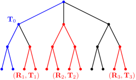
Figure 3: In order to enumerate, as described above we choose the blue, black and red parts of $\mathbf{T}$ in order.

which implies (3.17) with an appropriate choice of $\kappa_{1}$. This proves the claim.

Next we investigate $\mathcal{G}_{s}^{2}$ as in Definition 3.5. For Item (i), we first note that by the sub-Gaussian concentration of Bernoulli variables, it holds that each vertex in $G$ has degree at least $(1-\eta/8)np_{\eta}$ except with exponentially small probability. Furthermore, from Lemma 3.11 we also obtain that under any conditioning of $\mathcal{I}_{s-1}$, except with exponentially small probability we have for any $v\in V_{R}$, the total number of edges between $v$ and vertices in $V\setminus V_{\mathtt{M}}$ is no more than $(1+\eta/8)(n-|\mathtt{M}_{s}|)p_{\eta}$. Therefore, with probability $1-o(1)$ for each vertex $v\in V_{R}$ the number of neighbors in $V_{\mathtt{M}}$ is at least

$$(1-\eta/8)np_{\eta}-(1+\eta/8)(n-|\mathtt{M}_{s}|)p_{\eta}\geq(|\mathtt{M}_{s}|-\eta n/4)p_{\eta}\geq\eta np_{\eta}/4\,.$$

A similar argument applies for $V_{R}$ and we get that with probability $1-o(1)$, each $v\in V_{R}$ has at least $\eta np_{\eta}/4$ neighbors in $V_{R}$.

Provided with these degree lower bounds, the number of $\xi$-tuples in $\operatorname{CAND}_{s}$ is at least of order $(np_{\eta})^{\zeta}$. In order to get $\operatorname{GC}_{s}$, we still need to remove those $s$-bad tuples in $\operatorname{CAND}_{s}$, and it suffice to show that the total number of removed tuples is typically $o\big{(}(np_{\eta})^{\zeta}\big{)}$. By Markov’s inequality, we only need to show that $\mathbb{E}|\operatorname{CAND}_{s}\setminus\operatorname{GC}_{s}|=o\big{(}(np_{\eta})^{\xi}\big{)}$. Taking conditional expectation with respect to $\mathcal{I}_{s-1}$ and using the averaging over conditioning principle, we see

$$\mathbb{E}|\operatorname{CAND}_{s}\setminus\operatorname{GC}_{s}|=\mathbb{E}\Big{[}\sum_{\operatorname{L}\in\mathfrak{A}(\mathtt{M}_{s},\xi)}\mathbb{P}\big{[}\operatorname{L}\in\operatorname{CAND}_{s}\setminus\operatorname{GC}_{s}\mid\mathcal{I}_{s-1}\big{]}\Big{]}\,.$$ (3.45)

Denote $\mathfrak{A}_{s}$ as the set of tuples in $\mathfrak{A}(R_{s-1},\chi)$ with the first coordinate equals to $u_{s}$ (which is the minimal number in $R_{s-1}$), from the definition of $\operatorname{CAND}_{s}$ and a union bound we see

$$\mathbb{P}\big{[}\operatorname{L}\in\operatorname{CAND}_{s}\setminus\operatorname{GC}_{s}\mid\mathcal{I}_{s-1}\big{]}\leq\sum_{\operatorname{Q}\in\mathfrak{A}_{s}}\mathbb{P}\big{[}I_{G}(L)\Join_{G}Q,\operatorname{L}\notin\operatorname{GC}_{s}\mid\mathcal{I}_{s-1}\big{]}\,,$$ (3.46)

where $L,Q$ denote for $I_{G}(\operatorname{L}),I_{G}(\operatorname{Q})$, respectively. We further denote $T_{L,Q}$ for the tree that certifies the event $\{L\Join_{G}Q\}$. From Definition 3.3, $\operatorname{L}\notin\operatorname{GC}_{s}$ implies that there exists a subgraph $T^{*}\cong\mathbf{T}$ in $T_{L,Q}\cup GO_{s-1}$ with leaf set $L^{*}$, such that $E(T^{*})\cap E(T_{L,Q})\neq\emptyset$ and $I_{G}^{-1}(L^{*})\in\operatorname{EXP}_{t^{*}}$ for some $1\leq t^{*}\leq s-1$. We write $\operatorname{d}_{GO_{s-1}}$ for the graph distance on $GO_{s-1}$, then it is readily to see that the two tuples $\operatorname{L}=I_{G}^{-1}(L)=(l_{1},\dots,l_{\xi})$ and $\operatorname{L}^{*}=(l_{1}^{*},\dots,l_{\xi}^{*})$ must satisfy the following two properties:
(i) For any $i\in[\xi]$, there exists $j\in[\xi]$ such that $\operatorname{d}_{GO_{s-1}}(v_{l_{i}^{*}},v_{l_{j}})\leq\zeta$.
(ii) For at least two indices $p\in[\xi]$, there exists $q\in[\xi]$ such that $\operatorname{d}_{GO_{s-1}}(v_{l_{p}},v_{l_{q}^{*}})\leq\zeta$.
We denote by $\mathtt{L}(\operatorname{L})$ the collection of all $\xi$-tuples $\operatorname{L}^{*}\in\mathfrak{A}(\operatorname{M}_{s-1},\xi)$ that satisfy Property (i) above.

For any triple $(\operatorname{L},\operatorname{Q},\operatorname{L}^{*})$ with $\operatorname{L}^{*}\in\mathtt{L}(\operatorname{L})$, we divide the event $\operatorname{L}^{*}\in\operatorname{EXP}_{t^{*}}$ for some $1\leq t^{*}\leq s-1$ into two cases according to whether

$$t^{*}\in\mathtt{t}(\operatorname{L})\mbox{ where }\mathtt{t}(\operatorname{L})=\{t^{\prime}:d_{GO_{s-1}}(v_{u_{t^{\prime}}},v_{l_{i}})\leq\zeta\text{ for some }i\in[\xi]\}\,.$$ (3.47)

For the case that $t^{*}\notin\mathtt{t}(\operatorname{L})$, the tree that certifies $\operatorname{L}^{\prime}\in\operatorname{CAND}_{t^{*}}$ can not be fully contained in $T_{L,Q}\cup GO_{s-1}$. From Lemma 3.11 and the proof of Lemma 3.1 (see e.g., (3.10)), we see such case happens with probability $o(1)$ uniformly under any conditioning $\mathcal{I}_{s-1}\cup\{T_{L,Q}\subset G\}$. For the case that $t^{*}\in\mathtt{t}(\operatorname{L})$, we apply a union bound and thus we get

$$\mathbb{P}[L\Join_{G}Q,\operatorname{L}\notin\operatorname{GC}_{s}\mid\mathcal{I}_{s-1}]\leq \ o(1)\times\mathbb{P}[L\Join_{G}Q\mid\mathcal{I}_{s-1}]$$

$$+ \ \sum_{\operatorname{L}^{*}\in\mathtt{L}(\operatorname{L})}\sum_{t^{*}\in\mathtt{t}(\operatorname{L})}\mathbb{P}[L\Join_{G}Q,\operatorname{L}^{*}\in\operatorname{EXP}_{t^{*}}\mid\mathcal{I}_{s-1}]\,.$$

From Lemma 3.11 we see $\mathbb{P}[L\Join_{G}Q\mid\mathcal{I}_{s-1}]\leq p_{\eta}^{\zeta}$ for any realization of $\mathcal{I}_{s-1}$. Thus the first term above is $o(p_{\eta}^{\zeta})$. To treat the remaining terms, we note that
(a) $\operatorname{L}^{*}\in\operatorname{EXP}_{t^{*}}$ implies that $\operatorname{L}^{*}\in\bigcup_{1\leq t\leq s-1}\operatorname{SUC}_{t}$ or $\operatorname{L}^{*}\in\operatorname{FAIL}_{t^{*}}\setminus\bigcup_{1\leq t\leq s-1}\operatorname{SUC}_{t}$;
(b) if $\operatorname{L}^{*}\in\bigcup_{1\leq t\leq s-1}\operatorname{SUC}_{t}$, then from Property (ii) above,

$$\mbox{ there are two indecies $i,j\in\operatorname{L}$ such that $\operatorname{d}_{GO_{s-1}}(v_{i},v_{j})\leq 3\zeta$};\\$$ (3.48)

(c) $\{\operatorname{L}^{*}\in\operatorname{FAIL}_{t^{*}}\}=\{I_{t^{*}}=0\}\cup\{I_{t^{*}}=1,\operatorname{L}^{*}\prec\operatorname{L}_{t^{*}}\}$ (recall that $\operatorname{MT}_{t}=(\operatorname{L}_{t},\operatorname{Q}_{t},\operatorname{Q}_{t}^{\prime})$ for $1\leq t\leq s-1$ with $I_{t}=1$).
Combining these together, we see for each pair $(\operatorname{L},\operatorname{Q})$, any $\operatorname{L}^{*}\in\mathtt{L}(\operatorname{L})$ and any $t^{*}\in\mathtt{t}(\operatorname{L})$, it holds that $\mathbb{P}[L\Join_{G}Q,\operatorname{L}^{*}\in\operatorname{EXP}_{t^{*}}\mid\mathcal{I}_{s-1}]$ is bounded by $p_{\eta}^{\zeta}$ times

$$\ \mathbf{1}_{\{\operatorname{L}\text{ satisfies }\eqref{eq-L-condition-b}\}}+\mathbb{P}[X_{t}<\log n\mid\mathcal{I}_{s-1},L\Join_{G}Q]$$ (3.49)

$$+ \ \mathbb{P}[X_{t^{*}}\geq\log n,\operatorname{L}^{*}\notin\bigcup_{1\leq t\leq s-1}\operatorname{SUC}_{t},\operatorname{L}^{*}\prec\operatorname{L}_{t^{*}}\mid\mathcal{I}_{s-1},L\Join_{G}Q]\,.$$

In order to bound the second term in (3.49), note that if $\{X_{t}<\log n\}$ holds under $\mathcal{I}_{s-1}\cap\{L\Join_{G}Q\}$, then it also holds under $\mathcal{I}_{s-1}$ together with any other configuration on the set $E(T_{L,Q})$. Thus,

$$\mathbb{P}[X_{t^{*}}<\log n\mid\mathcal{I}_{s-1},L\Join_{G}Q]\leq\mathbb{P}[X_{t^{*}}<\log n\mid\mathcal{I}_{s-1}]\,.$$

In order to bound the third term in (3.49), denote $\operatorname{Avai}_{t}$ for the (random) set of tuples in $\operatorname{CAND}_{t}$ that can be successfully matched, $1\leq t\leq s-1$. Then $|\operatorname{Avai}_{t}|=X_{t}$ and the conditional law of $\prec$ given $\mathcal{I}_{s-1}\cap\{L\Join_{G}Q\}$ is uniform conditioned on the following event:

$$\{\operatorname{L}_{t}\text{ is $\prec$-minimal among }\operatorname{Avai}_{t},\mbox{ for all }1\leq t\leq s-1\text{ with }I_{t}=1\}\,.$$

In particular, under such conditioning, for $\operatorname{L}^{*}\notin\bigcup_{1\leq t\leq s-1}\operatorname{SUC}_{t}$ it holds with conditional probability $1/X_{t^{*}}$ that $\operatorname{L}^{*}\prec\operatorname{L}_{t^{*}}$. As a result, the third term is bounded by $(\log n)^{-1}=o(1)$.

Summing over all $(\operatorname{L},\operatorname{Q})$ and combining all the arguments above altogether, we get

$$\sum_{\operatorname{L}\in\mathfrak{A}(\mathtt{M}_{s},\xi)} \mathbb{P}\big{[}\operatorname{L}\in\operatorname{CAND}_{s}\setminus\operatorname{GC}_{s}\mid\mathcal{I}_{s-1}\big{]}$$

$$\leq\sum_{\operatorname{L}\in\mathfrak{A}(\mathtt{M}_{s},\xi)}\sum_{\operatorname{Q}\in\mathfrak{A}_{s}}\sum_{\operatorname{L}^{*}\in\mathtt{L}(\operatorname{L})}\sum_{t^{*}\in\mathtt{t}(\operatorname{L})} p_{\eta}^{\zeta}\Big{(}o(1)+\mathbf{1}_{\{\operatorname{L}\text{ satisfies }\eqref{eq-L-condition-b}\}}+\mathbb{P}[X_{t^{*}}<\log n\mid\mathcal{I}_{s-1}]\Big{)}\,.$$ (3.50)

We now bound the number of effective terms in the summation of (3.3). Clearly, $|\mathfrak{A}(\mathtt{M}_{t},\xi)|\leq n^{\xi}$ and $|\mathfrak{A}_{s}|\leq n^{\chi-1}$. In addition, by (3.4) we see both $|\mathtt{L}(\operatorname{L})|$ and $|\mathtt{t}(\operatorname{L})|$ are uniformly bounded for $\operatorname{L}\in\mathfrak{A}(\mathtt{M}_{s},\xi)$. Furthermore, the number of $\operatorname{L}\in\mathfrak{A}(\mathtt{M}_{s},\xi)$ that satisfy (3.48) is of order $O\big{(}n^{\xi-1}\big{)}$, and for each $1\leq t^{*}\leq s-1$ the number of tuples $\operatorname{L}\in\mathfrak{A}(\mathtt{M}_{s},\xi)$ such that $\mathtt{t}(\operatorname{L})$ contains $t^{*}$ is also of order $O\big{(}n^{\xi-1}\big{)}$ (since some vertex in $L$ must be close to $v_{u_{t}}$ on the graph $GO_{s-1}$). Altogether, we see the right hand side of (3.3) is upper-bounded by (recall that $\zeta=\xi+\chi-1$)

$$O\big{(}n^{\zeta}\big{)}\times o\big{(}p_{\eta}^{\zeta}\big{)}+O\big{(}n^{\zeta-1}\big{)}\times p_{\eta}^{\zeta}+O\big{(}n^{\zeta-1}\big{)}\times p_{\eta}^{\zeta}\times\sum_{1\leq t^{*}\leq s-1}\mathbb{P}[X_{t^{*}}<\log n\mid\mathcal{I}_{s-1}]\,.$$

Averaging over $\mathcal{I}_{s-1}$ and recalling (3.45) and (3.3), we obtain that

$$\mathbb{E}|\operatorname{CAND}_{s}\setminus\operatorname{GC}_{s}|=o\big{(}(np_{\eta})^{\zeta}\big{)}+O\big{(}n^{\zeta-1}p_{\eta}^{\zeta}\big{)}\sum_{1\leq t^{*}\leq s-1}\mathbb{P}[X_{t^{*}}<\log n]\stackrel{{\scriptstyle\eqref{eq;good-step-est}}}{{=}}o\big{(}(np_{\eta})^{\zeta}\big{)}\,,$$

as desired. This implies that Item (i) of $\mathcal{G}_{s}^{2}$ in Definition 3.5 holds with probability $1-o(1)$.

Finally, we treat Item (ii) of $\mathcal{G}_{s}^{2}$ in Definition 3.5 and it suffices to show that it holds on the event $\mathcal{G}$. Since each tuple in $\operatorname{GC}_{s}$ corresponds to a subgraph $T\cong\mathbf{T}$ in $G$ rooted at $v_{u_{s}}$, (3.44) implies that $|\operatorname{GC}_{s}|=O\big{(}(np_{\eta})^{\zeta}\big{)}$. For each fixed $\operatorname{L}_{i}\in\operatorname{GC}_{s}$ and a nonempty subset $\mathbf{R}\subset\mathbf{L}$, we bound the number of $\operatorname{L}_{j}\in\operatorname{GC}_{s}$ such that $(\operatorname{L}_{i},\operatorname{L}_{j})\in\operatorname{IP}_{s}(\mathbf{R})$ as follows: each such $\operatorname{L}_{j}$ corresponds to a subgraph ${T}\cong\mathbf{T}$ of ${G}$ with leaves in $\mathbf{R}$ mapped to a fixed subset in $V(G)$ under the isomorphism. In order to bound the enumeration for such ${T}$, we use the following two-step procedure to choose ${T}$:

• choose a subgraph ${T}_{0}\cong\mathbf{Span}(\mathbf{R})$ of ${G}$ with leaves in $\mathbf{R}$ mapped to a fixed subset in $V(G)$ under the isomorphism;

• choose ${T}\cong\mathbf{T}$ of ${G}$ with $\mathbf{Span}(\mathbf{R})$ mapped to $T_{0}$ under the isomorphism.

Thus, by Definition 3.8 and by (3.44), the number of choices for such $T$ is $O\big{(}\mathbb{D}(\mathbf{Span}(\mathbf{R}))\times(np_{\eta})^{|E(\mathbf{T})\setminus E(\mathbf{Span}(\mathbf{R}))|}\big{)}$ on $\mathcal{G}$, and thus Item (ii) of $\mathcal{G}_{s}^{2}$ holds with probability $1-o(1)$. This completes the proof of Proposition 2.6. ∎

References

- [1] E. Abbe. Community detection and stochastic block models: recent developments. J. Mach. Learn. Res., 18:Paper No. 177, 86, 2017.
- [2] A. S. Bandeira, A. Perry, and A. S. Wein. Notes on computational-to-statistical gaps: predictions using statistical physics. Port. Math., 75(2):159–186, 2018.
- [3] B. Barak, C.-N. Chou, Z. Lei, T. Schramm, and Y. Sheng. (nearly) efficient algorithms for the graph matching problem on correlated random graphs. In Advances in Neural Information Processing Systems, volume 32. Curran Associates, Inc., 2019.
- [4] A. Berg, T. Berg, and J. Malik. Shape matching and object recognition using low distortion correspondences. In 2005 IEEE Computer Society Conference on Computer Vision and Pattern Recognition (CVPR’05), volume 1, pages 26–33 vol. 1, 2005.
- [5] M. Bozorg, S. Salehkaleybar, and M. Hashemi. Seedless graph matching via tail of degree distribution for correlated erdos-renyi graphs. Preprint, arXiv:1907.06334.
- [6] T. Cour, P. Srinivasan, and J. Shi. Balanced graph matching. In B. Schölkopf, J. Platt, and T. Hoffman, editors, Advances in Neural Information Processing Systems, volume 19. MIT Press, 2006.
- [7] D. Cullina and N. Kiyavash. Exact alignment recovery for correlated Erdos-Rényi graphs. Preprint, arXiv:1711.06783.
- [8] D. Cullina and N. Kiyavash. Improved achievability and converse bounds for erdos-renyi graph matching. In Proceedings of the 2016 ACM SIGMETRICS International Conference on Measurement and Modeling of Computer Science, SIGMETRICS ’16, page 63–72, New York, NY, USA, 2016. Association for Computing Machinery.
- [9] D. Cullina, N. Kiyavash, P. Mittal, and H. V. Poor. Partial recovery of erdos-rényi graph alignment via -core alignment. SIGMETRICS ’20, page 99–100, New York, NY, USA, 2020. Association for Computing Machinery.
- [10] O. E. Dai, D. Cullina, N. Kiyavash, and M. Grossglauser. Analysis of a canonical labeling algorithm for the alignment of correlated erdos-rényi graphs. Proc. ACM Meas. Anal. Comput. Syst., 3(2), jun 2019.
- [11] A. Dembo, A. Montanari, and S. Sen. Extremal cuts of sparse random graphs. Ann. Probab., 45(2):1190–1217, 2017.
- [12] J. Ding and H. Du. Detection threshold for correlated erdos-renyi graphs via densest subgraph. Preprint, arXiv:2203.14573.
- [13] J. Ding and H. Du. Matching recovery threshold for correlated random graphs. Preprint, arXiv:2205.14650.
- [14] J. Ding, Z. Ma, Y. Wu, and J. Xu. Efficient random graph matching via degree profiles. Probab. Theory Related Fields, 179(1-2):29–115, 2021.
- [15] Z. Fan, C. Mao, Y. Wu, and J. Xu. Spectral graph matching and regularized quadratic relaxations II: Erdos-rényi graphs and universality. Preprint, arXiv:1907.08883.
- [16] Z. Fan, C. Mao, Y. Wu, and J. Xu. Spectral graph matching and regularized quadratic relaxations: Algorithm and theory. In Proceedings of the 37th International Conference on Machine Learning, volume 119 of Proceedings of Machine Learning Research, pages 2985–2995. PMLR, 13–18 Jul 2020.
- [17] S. Feizi, G. Quon, M. Medard, M. Kellis, and A. Jadbabaie. Spectral alignment of networks. Preprint, arXiv:1602.04181.
- [18] D. Gamarnik. The overlap gap property: A topological barrier to optimizing over random structures. Proceedings of the National Academy of Sciences, 118(41):e2108492118, 2021.
- [19] D. Gamarnik and I. Zadik. The landscape of the planted clique problem: Dense subgraphs and the overlap gap property. Preprint, arXiv:1904.07174.
- [20] L. Ganassali and L. Massoulié. From tree matching to sparse graph alignment. In J. Abernethy and S. Agarwal, editors, Proceedings of Thirty Third Conference on Learning Theory, volume 125 of Proceedings of Machine Learning Research, pages 1633–1665. PMLR, 09–12 Jul 2020.
- [21] A. Haghighi, A. Ng, and C. Manning. Robust textual inference via graph matching. In Proceedings of Human Language Technology Conference and Conference on Empirical Methods in Natural Language Processing, pages 387–394, Vancouver, British Columbia, Canada, Oct 2005.
- [22] G. Hall and L. Massoulié. Partial recovery in the graph alignment problem. Preprint, arXiv:2007.00533.
- [23] E. Kazemi, S. H. Hassani, and M. Grossglauser. Growing a graph matching from a handful of seeds. Proc. VLDB Endow., 8(10):1010–1021, jun 2015.
- [24] D. Kunisky, A. S. Wein, and A. S. Bandeira. Notes on computational hardness of hypothesis testing: Predictions using the low-degree likelihood ratio. Preprint, arXiv:1907.11636.
- [25] V. Lyzinski, D. E. Fishkind, and C. E. Priebe. Seeded graph matching for correlated Erdos-Rényi graphs. J. Mach. Learn. Res., 15:3513–3540, 2014.
- [26] P. Manurangsi, A. Rubinstein, and T. Schramm. The Strongish Planted Clique Hypothesis and Its Consequences. In J. R. Lee, editor, 12th Innovations in Theoretical Computer Science Conference (ITCS 2021), volume 185 of Leibniz International Proceedings in Informatics (LIPIcs), pages 10:1–10:21, Dagstuhl, Germany, 2021. Schloss Dagstuhl–Leibniz-Zentrum für Informatik.
- [27] C. Mao, M. Rudelson, and K. Tikhomirov. Exact matching of random graphs with constant correlation. Preprint, arXiv:2110.05000.
- [28] C. Mao, Y. Wu, J. Xu, and S. H. Yu. Testing network correlation efficiently via counting trees. Preprint, arXiv:2110.11816.
- [29] M. Mitzenmacher and E. Upfal. Probability and Computing: Randomized Algorithms and Probabilistic Analysis. Cambridge University Press, USA, 2005.
- [30] A. Montanari. Optimization of the sherrington-kirkpatrick hamiltonian. In 2019 IEEE 60th Annual Symposium on Foundations of Computer Science (FOCS), pages 1417–1433, 2019.
- [31] A. Montanari and S. Sen. Semidefinite programs on sparse random graphs and their application to community detection. In STOC’16—Proceedings of the 48th Annual ACM SIGACT Symposium on Theory of Computing, pages 814–827. ACM, New York, 2016.
- [32] E. Mossel and J. Xu. Seeded graph matching via large neighborhood statistics. Random Structures Algorithms, 57(3):570–611, 2020.
- [33] A. Narayanan and V. Shmatikov. Robust de-anonymization of large sparse datasets. In 2008 IEEE Symposium on Security and Privacy (sp 2008), pages 111–125, 2008.
- [34] A. Narayanan and V. Shmatikov. De-anonymizing social networks. In 2009 30th IEEE Symposium on Security and Privacy, pages 173–187, 2009.
- [35] R. Nenadov, A. Steger, and P. Su. An O(N) time algorithm for finding Hamilton cycles with high probability. In 12th Innovations in Theoretical Computer Science Conference, volume 185 of LIPIcs. Leibniz Int. Proc. Inform., pages Art. No. 60, 17. Schloss Dagstuhl. Leibniz-Zent. Inform., Wadern, 2021.
- [36] P. Pedarsani and M. Grossglauser. On the privacy of anonymized networks. In Proceedings of the 17th ACM SIGKDD International Conference on Knowledge Discovery and Data Mining, KDD ’11, page 1235–1243, New York, NY, USA, 2011. Association for Computing Machinery.
- [37] P. Raghavendra, T. Schramm, and D. Steurer. High dimensional estimation via sum-of-squares proofs. In Proceedings of the International Congress of Mathematicians—Rio de Janeiro 2018. Vol. IV. Invited lectures, pages 3389–3423. World Sci. Publ., Hackensack, NJ, 2018.
- [38] F. Shirani, S. Garg, and E. Erkip. Seeded graph matching: Efficient algorithms and theoretical guarantees. In 2017 51st Asilomar Conference on Signals, Systems, and Computers, pages 253–257, 2017.
- [39] R. Singh, J. Xu, and B. Berger. Global alignment of multiple protein interaction networks with application to functional orthology detection. Proceedings of the National Academy of Sciences of the United States of America, 105:12763–8, 10 2008.
- [40] J. Spencer. Counting extensions. J. Combin. Theory Ser. A, 55(2):247–255, 1990.
- [41] E. Subag. Following the ground states of full-RSB spherical spin glasses. Comm. Pure Appl. Math., 74(5):1021–1044, 2021.
- [42] J. T. Vogelstein, J. M. Conroy, V. Lyzinski, L. J. Podrazik, S. G. Kratzer, E. T. Harley, D. E. Fishkind, R. J. Vogelstein, and C. E. Priebe. Fast approximate quadratic programming for graph matching. PLOS ONE, 10(4):1–17, 04 2015.
- [43] Y. Wu and J. Xu. Statistical Problems with Planted Structures: Information-Theoretical and Computational Limits, page 383–424. Cambridge University Press, 2021.
- [44] Y. Wu, J. Xu, and S. H. Yu. Settling the sharp reconstruction thresholds of random graph matching. Preprint, arXiv:2102.00082.
- [45] Y. Wu, J. Xu, and S. H. Yu. Testing correlation of unlabeled random graphs. Preprint, arXiv:2008.10097.
- [46] L. Yartseva and M. Grossglauser. On the performance of percolation graph matching. In Proceedings of the First ACM Conference on Online Social Networks, COSN ’13, page 119–130, New York, NY, USA, 2013. Association for Computing Machinery.
- [47] L. Zdeborová and F. Krzakala. Statistical physics of inference: thresholds and algorithms. Advances in Physics, 65(5):453–552, 2016.