Activity-aware Human Mobility Prediction with Hierarchical Graph Attention Recurrent Network

Abstract

Human mobility prediction is a fundamental task essential for various applications, including urban planning, location-based services and intelligent transportation systems. Existing methods often ignore activity information crucial for reasoning human preferences and routines, or adopt a simplified representation of the dependencies between time, activities and locations. To address these issues, we present Hierarchical Graph Attention Recurrent Network (Hgarn) for human mobility prediction. Specifically, we construct a hierarchical graph based on all users’ history mobility records and employ a Hierarchical Graph Attention Module to capture complex time-activity-location dependencies. This way, Hgarn can learn representations with rich human travel semantics to model user preferences at the global level. We also propose a model-agnostic history-enhanced confidence (MaHec) label to focus our model on each user’s individual-level preferences. Finally, we introduce a Temporal Module, which employs recurrent structures to jointly predict users’ next activities (as an auxiliary task) and their associated locations. By leveraging the predicted future user activity features through a hierarchical and residual design, the accuracy of the location predictions can be further enhanced. For model evaluation, we test the performances of our Hgarn against existing SOTAs in both the recurring and explorative settings. The recurring setting focuses on assessing models’ capabilities to capture users’ individual-level preferences, while the results in the explorative setting tend to reflect the power of different models to learn users’ global-level preferences. Overall, our model outperforms other baselines significantly in all settings based on two real-world human mobility data benchmarks.

I Introduction

Human mobility is critical for various downstream applications such as urban planning, location-based services and intelligent transportation systems. The ability to model and accurately predict future human mobility can inform us about important public policy decisions for society’s betterment, such as managing traffic congestion, promoting social integration, and maximizing productivity [1]. Central to human mobility modeling is the problem of next location prediction, i.e., the prediction of where an individual is going next, which has received great attention. On the one hand, the increasing prevalence of mobile devices and popularity of location-based social networks (LBSNs) provide unprecedented data sources for mining individual-level mobility traces and preferences [2]. On the other hand, the advancement of AI and machine learning offers a plethora of analytical tools for modeling human mobility. These innovations greatly enhance human mobility modeling in the past decade, especially for the next location prediction.

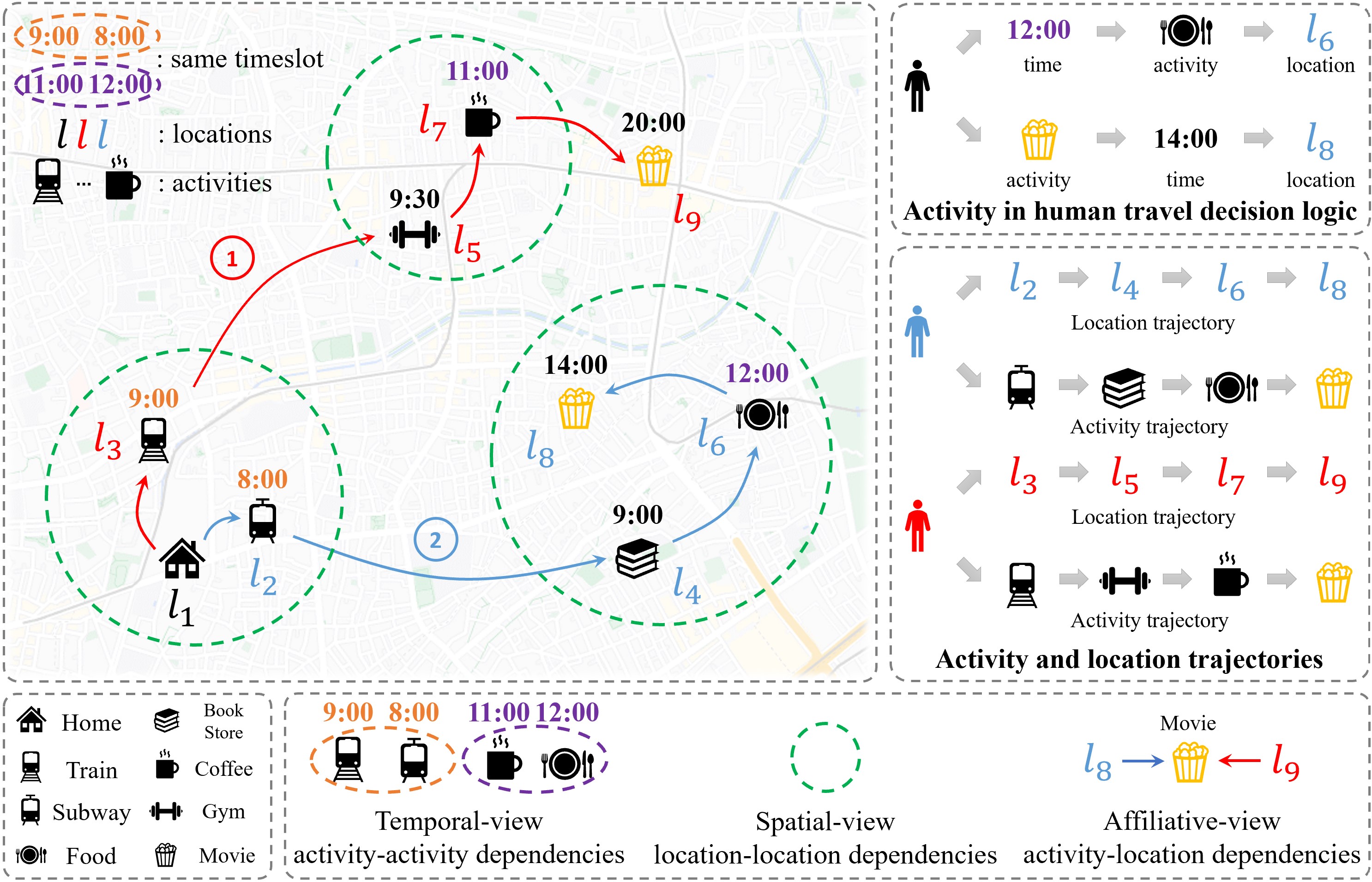
Figure 1: An illustration of two human mobility trajectories. Activities are essential in affecting human travel decisions.

Traditional approaches to human mobility analysis typically used Markov Chains (Mc) [3, 4, 5] to model transition patterns over location sequences. Later, recurrent neural networks (Rnn) [6] demonstrated better predictive power than Mc-based methods, including pioneering works that employed recurrent structures to model temporal periodicity [7] and spatial regularity [8]. Some other Rnn-based methods incorporate spatial and temporal contexts [9, 10] into the Rnn update process to boost model performances. In addition, due to the great success of the Transformer architecture [11], the attention mechanism has also been adopted to better model sequences and obtain good prediction results [12, 13]. In recent years, graph-based approaches leveraged graph representation learning [14, 15] and graph neural networks (Gnns) [16] to model user preferences [17] and spatial-temporal relationships [18, 12] between locations, obtaining rich representations [19, 20] to improve the performance of next location prediction. While most studies focus on predicting human mobility based on individual location sequences, neglecting the inherent travel behavior structure and associated activity data, and downplaying the integral interplay between activity participation and location visitation behaviors. Classic travel behavior theories suggest that an individual’s location visits are influenced by their daily activity patterns [21]. Given the greater accessibility of human activity data and the fewer activity categories compared to location options, incorporating these activity dynamics into human mobility modeling offers a behaviorally insightful and computationally effective approach.

Figure 1 shows several human mobility trajectories reflecting time-activity-location dependencies. For example, when the time is approaching noon, one user may dine at a nearby restaurant, and another may go to the movie theater for a specific starting time, which illustrates that activities are usually scheduled according to the time of day. People typically make location decisions based on the intended activities, and considering activity information can lead to better predictability of human mobility. However, few works have considered adding activity information (e.g., location categories) for next location prediction. Yu et al. [22] used activities along with spatial distances to reduce search space (i.e., candidate locations). Huang et al. [23] proposed a Cslsl which comprises an Rnn-based structure [24], where the time, activity, and location are predicted sequentially, to model human travel decision logic. However, the design of Cslsl oversimplifies the time-activity-location dependencies. Given data sparsity and behavioral uncertainties [25], the time prediction tends to be more challenging [26], which may further compromise the prediction of activities and locations.

Based on the above observations, a suitable human next location predictor should: (1) take into account human activities when predicting their next locations and leverage the predicted future human activity information to enhance location prediction, and (2) effectively manage intricate time-activity-location dependencies while circumventing the difficulty in time prediction under data sparsity and uncertain human behaviors. To our best knowledge, no prior work has attempted to model the sophisticated time-activity-location dependencies to enhance next location prediction. In this paper, we present Hierarchical Graph Attention Recurrent Network (Hgarn) for next location prediction. Initially, we construct a hierarchical graph based on time-activity-location all users’ records and employ a Hierarchical Graph Attention Module to capture complex temporal-view activity-activity, affiliated-view activity-location, spatial-view location-location dependencies. This way, Hgarn can learn representations with rich human travel semantics to model user preferences at the global level. Correspondingly, a model-agnostic history-enhanced confidence (MaHec) label is proposed to guide our model to learn each user’s individual-level preferences. We finally introduce a Temporal Module that takes the sequence of user embeddings combined with the learned hierarchical graph representations as input to jointly predict a user’s next activity (as the auxiliary task) and location. Specifically, the former can be hierarchically and residually incorporated into the latter. Through such design, Hgarn can leverage the learned time-activity-location dependencies to benefit both global- and individual-level human mobility modeling, and use predicted next activity distribution to facilitate model performance for next location prediction.

In summary, our paper makes the following contributions:

• We propose a Hierarchical Graph that incorporates human activity information to represent the temporal-view activity-activity, affiliated-view activity-location, spatial-view location-location dependencies. To the best of our knowledge, among the few approaches incorporating activity information into next location prediction, this is the first work to model the dependencies of time, activities and locations by leveraging a Hierarchical Graph.

• We design a activity-aware Hierarchical Graph Attention Recurrent Network (i.e., Hgarn), which contains a hierarchical graph attention module to model dependencies between time, activities, and locations to capture users’ global-level preferences, and a temporal module to incorporate the hierarchical graph representations into sequence modeling and utilize next activity prediction to boost next location prediction.

• We introduce a simple yet effective model-agnostic history-enhanced confidence (MaHec) label to guide the model learning of each user’s individual-level preferences, which enables the model to focus more on relevant locations in their history trajectories when predicting their next locations.

• Extensive experiments are conducted using two real-world LBSN check-in datasets. Specifically, we evaluate the prediction performance of Hgarn against existing SOTAs in the main, recurring, and explorative settings. Our work is the first to separately evaluate next location prediction performance in these settings. The results show that Hgarn can significantly outperform existing methods in all experimental settings.

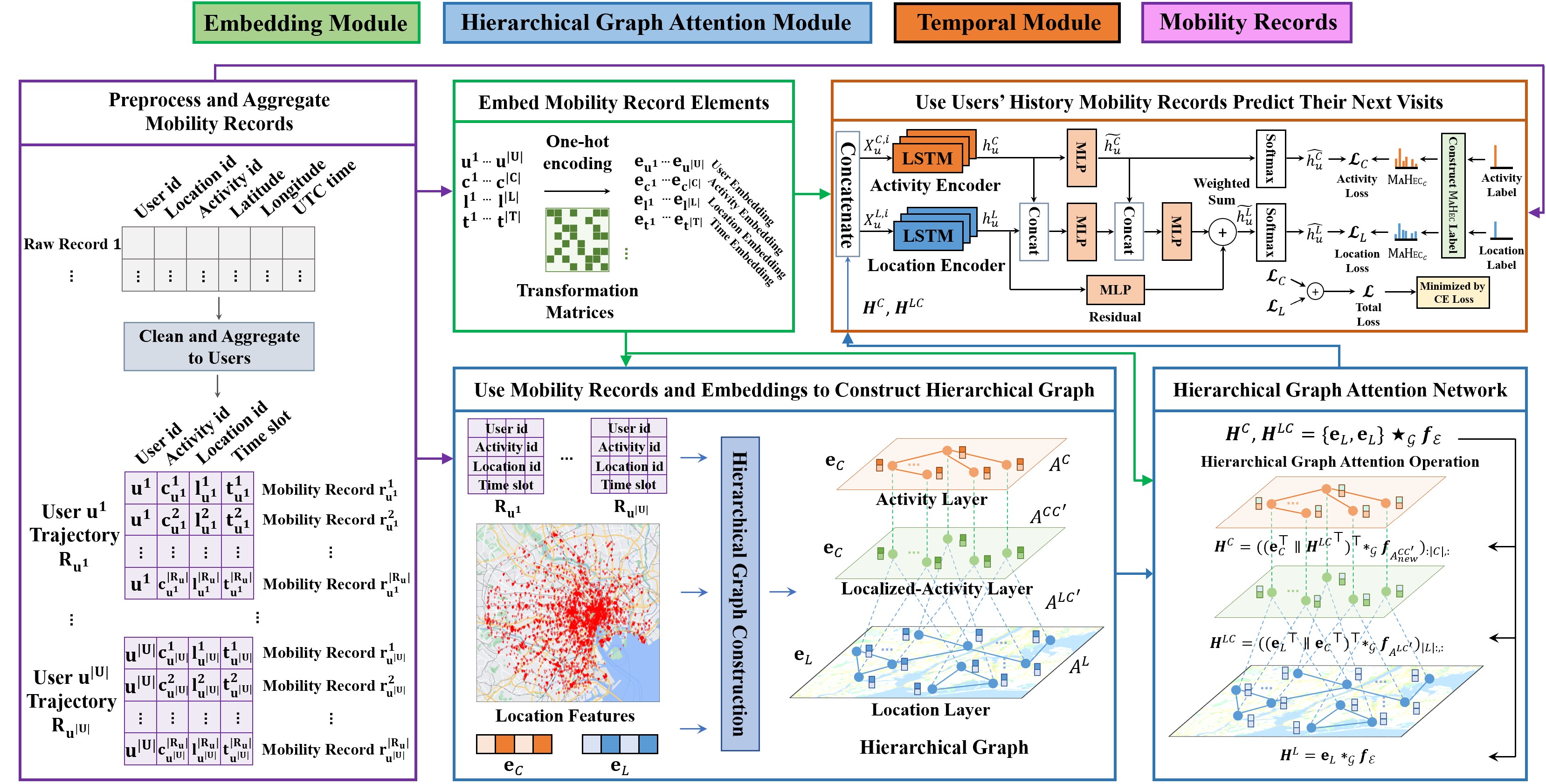
Figure 2: A workflow of the proposed Hgarn.

II Related work

II-A Next Location Prediction

Next location prediction is essentially about sequence modeling since successive location visits are usually correlated [27, 28]. Traditional Mc-based methods often incorporate other techniques, such as matrix factorization [4] and activity-based modeling [5], to capture mobility patterns and make predictions. However, Mc-based methods are limited in capturing long-term dependencies or predicting exploratvie human mobility.

Deep learning-based approaches consider the next location prediction problem as a sequence-to-sequence task and obtain better prediction results than traditional methods. The majority of existing deep learning models are based on Rnn [6, 29]. Strnn [9] is a pioneering work that incorporates spatial-temporal features between consecutive human visits into Rnn models to predict human mobility. Stgn [30] adds spatial and temporal gates to Lstm to learn users interests. Flashback [8] leverages spatial and temporal intervals to compute aggregated past Rnn hidden states for predictions. Lstpm [10] introduces a non-local network and a geo-dilated Lstm to model users’ long- and short-term preferences. Some approaches use the attention mechanism to improve their performances. DeepMove [7] leveraged attention mechanisms combined with an Rnn module to capture users’ long- and short-term preferences. Arnn [13] uses a knowledge graph to find related neighboring locations and model the sequential regularity of check-ins through attentional Rnn. Stan [12] extracts relative spatial-temporal information between consecutive and non-consecutive locations through a spatio-temporal attention network for locations predictions. In addition, some efforts incorporate contextual information [31] such as geographical information [32], dynamic-static [33], text content about locations [34] into sequence modeling.

Recently, graph-based models have been designed to enrich contextual features, which can reflect global preferences. LBSN2Vec [14] performs random walks on a hypergraph to learn embeddings for next location and friendship predictions. STP-UDGAT [17] uses Gat to learn location relationships from both local and global views based on constructed spatial, temporal, and preference graphs. Hmt-Grn [35] learned several user-region matrices of different granularity levels to alleviate the data sparsity issue and efficiently predict the next location. Gcdan [18] uses dual attention to model the high-order sequential dependencies and Gcn to mitigate the data sparsity issue. Graph-Flashback [20] uses knowledge graph embedding to construct transition graphs, and applies Gcn to refine graph representations and combines with Flashback to make predictions.

Some other works focused on different aspects, [36] focus on activity trajectory generation to model the diffusion patterns of the COVID-19 pandemic, and [37] leverages Gail [38] to simulate human daily activities. Activity-aware methods like [39] model the activities with a weighted category hierarchy (WCH), CatDM [22] uses activities along with spatial distances to reduce search space, Cslsl [23] proposed an Rnn-based causal structure to capture human travel decision logic. However, most existing methods ignore the activity information and cannot effectively model the time-activity-location dependencies, which are essential for predicting and understanding human mobility.

II-B Hierarchical Graph Neural Network

The Hierarchical Graph Neural Network (HGnn) is a family of graph neural network (Gnn) models that have gained significant attention in recent years due to their ability to capture complex dependencies in data using hierarchical structures. HGnn has been applied to various fields such as visual relationship detection [40, 41, 42], and urban forecasting applications such as parking availability [43], air quality [44], road network representation learning [45], real estate appraisal [46], and socioeconomic indicators prediction [47]. However, each model has its own structure design and graph construction mechanisms based on their specific application scenarios, resulting in fundamentally different architectures.

One relevant HGnn-based approach for next location prediction is Hmt-Grn [35], which partitions the spatial map and performs a Hierarchical Beam Search (Hbs) on different regions and POI distributions to hierarchically reduce the search space for accurate predictions. In contrast, our proposed Hgarn is an activity-based model designed for predicting the next location by capturing complex time-activity-location dependencies. Hgarn construct a hierarchical graph based on human activities and utilizes a manually defined attention-based message passing mechanism with hierarchies to effectively capture mixed information and predict the next location for each user. This activity-based design is unique and distinguishes Hgarn from other HGnn-based models.

III Preliminaries

This section introduces definitions relevant to this study and then formulates the next location prediction problem.

We use notations $U=\left\{u^{i}\right\}_{i=1}^{|U|}$, $L=\{l^{i}\}_{i=1}^{|L|}$, $C=\{c^{i}\}_{i=1}^{|C|}$, and $T=\{t^{i}\}_{i=1}^{|T|}$ to denote the sets of users, locations, activities and time series, respectively. In particular, we denote a user $u\in U$’s sets of locations, activities and time series in a temporal order as $L_{u}=\{l^{i}_{u}\}_{i=1}^{|L_{u}|}$, $C_{u}=\{c^{i}_{u}\}_{i=1}^{|C_{u}|}$, and $T_{u}=\{t^{i}_{u}\}_{i=1}^{|T_{u}|}$, where $\delta_{u}^{i}$ may not equal to $\delta^{i}$, $\delta\in\{U,L,C,T\}$.

Definition 1 (Mobility Record).

We use the notation $r$ to denote a single human mobility record. Specifically, the $i$th record of a given user $u\in U$ is represented by a tuple $r_{u}^{i}=(u,c_{u}^{i},l_{u}^{i},t_{u}^{i})$. Each record tuple comprises a user $u\in U$, an activity $c_{u}^{i}\in C_{u}$, a location $l_{u}^{i}\in L_{u}$ and the visit time $t_{u}^{i}\in T_{u}$.

Definition 2 (Trajectory).

A trajectory is a sequence of mobility records that belongs to a user $u\in U$, denoted by $R_{u}=\{r_{u}^{i}\}_{i=1}^{|R_{u}|}$. Each trajectory $R_{u}$ can be divided into a history trajectory $R_{u}^{his}=\{r_{u}^{i}\}_{i=1}^{|R_{u}|-1}$ and the final record $r_{u}^{|R_{u}|}$. In this way, we can obtain the user $u$’s activity trajectories $R_{u}^{C}={\{c_{u}^{i}\}}_{i=1}^{|R_{u}|}$, location trajectories $R_{u}^{L}={\{l_{u}^{i}\}}_{i=1}^{|R^{u}|}$, and time trajectories $R_{u}^{T}={\{t_{u}^{i}\}}_{i=1}^{|R_{u}|}$ with their history trajectories $R_{u}^{C,his}$, $R_{u}^{L,his}$ and $R_{u}^{T,his}$.

Problem 1 (Next Location Prediction).

Given a user $u\in U$’s history trajectory $R_{u}^{his}$ as input, we consider $u$’s next record as its future state. The human mobility prediction task $\mathcal{T}$ maps $u$’s history trajectory $R_{u}^{his}$ to $u$’s next location $l_{u}^{|R_{u}|}$ in the future. The above-described process can be summarized as follows:

$$R_{u}^{his}\stackrel{{\scriptstyle\mathcal{T}(\cdot;\theta)}}{{\longrightarrow}}l_{u}^{|R_{u}|},$$ (1)

where $\theta$ is the parameters of mapping $\mathcal{T}$.

IV Methodology

Hgarn’s workflow is demonstrated in Figure 2. The raw data is first encoded in the embedding Module and then input to the hierarchical graph attention module to model multi-dependencies. Finally, the user’s personalized embeddings are fused with the learned hierarchical graph representations and input to the Temporal module to make predictions. We will elaborate on the details of our Hgarn.

IV-A Embedding Module

We first introduce our embedding module, which aims to assign trainable embeddings to each unique mobility record element for neural network training, i.e., the user, activity, location and time. It is worth noting that all these elements are discrete values except for time, and it is necessary to split the continuous time into discrete intervals to facilitate the encoding of time. In this work we discretize the 24 hours of the day into $|T^{h}|$ time slots $T^{h}=\{h\}_{h=1}^{|T^{h}|}$ and another variable $T^{w}=\{w\}_{w=1}^{|T^{w}|}$ indicating the day of the week. Note that all $t\in T$ can be written in the form of $t=(h,w)$. We obtain the embeddings of each user, activity, location and time $\bm{e}_{u}\in\mathbb{R}^{d^{u}}$, $\bm{e}_{c},\bm{e}_{l}\in\mathbb{R}^{d}$, $\bm{e}_{t}\in\mathbb{R}^{d^{t}}$ by multiplying their one-hot vectors with the corresponding trainable transformation matrices, where $d^{u}$, $d$ and $d^{t}$ represent embedding dimensions. $\bm{e}_{U}\in\mathbb{R}^{|U|\times{d^{u}}}$, $\bm{e}_{C}\in\mathbb{R}^{|C|\times{d}}$, $\bm{e}_{L}\in\mathbb{R}^{|L|\times{d}}$ and $\bm{e}_{T}\in\mathbb{R}^{|T|\times{d^{t}}}$ are used to denote the embedding matrices for the user, activity, location and time, respectively. $\bm{e}_{r_{u}^{i}}=\left(\bm{e}_{u},\bm{e}_{c_{u}^{i}},\bm{e}_{l_{u}^{i}},\bm{e}_{t_{u}^{i}}\right)$ is used to denote a user $u$’s embeddings of $i$th record.

IV-B Hierarchical Graph Attention Module

To model the complex dependencies between human activities and locations, the hierarchical graph attention module is designed with two parts: hierarchical graph construction and hierarchical graph attention networks on the graph for multi-dependencies modeling.

IV-B1 Hierarchical Graph Construction

The urban spatial network can be represented as a graph structure. Graph neural networks provide an effective way to learn graph representation and model node-to-node dependencies [48, 49]. We model the location-location, location-activity, and activity-activity dependencies using a well-designed graph attention operation on a hierarchical graph.

The hierarchical graph consists of three layers: the location layer, the localized-activity layer, and the activity layer. The localized-activity layer is employed to suppress noise aggregated from the location layer. We formally describe the hierarchical graph with notation $\mathcal{G}=(\mathcal{V},\mathcal{E})$, where $\mathcal{V}$ $=$ $\mathcal{V}^{L}\cup\mathcal{V}^{C}\cup\mathcal{V}^{C^{\prime}}$ and $\mathcal{E}=\{A^{L}$,$A^{C}$,$A^{LC^{\prime}}$,$A^{CC^{\prime}}\}$. Specifically, $\mathcal{V}^{L}$ and $\mathcal{V}^{C}$ represents the location node-set and the activity node-set. $\mathcal{V}^{C^{\prime}}$ indicates the localized-activity node-set. $E$ comprises four adjacency matrices that denote connectivity between (1) two location nodes, (2) two activity nodes, (3) a location node and a localized-activity node, (4) an activity node and a localized-activity node.

For the location adjacency matrix $A^{L}$, we utilize the geographical distance to determine whether two nodes are linked to indicate spatial adjacency. We employ the haversine formula (which is used to calculate distances between locations using latitude and longitude coordinates.) to compute distances between locations. Given $l^{i}$ and $l^{j}$ and their GPS data, $A^{L}\in\mathbb{R}^{|L|\times|L|}$ is as:

$$A^{L}_{l^{i},l^{j}}=\begin{cases}1,&Haversine\left(\text{GPS}^{i},\text{GPS}^{j}\right)<D^{h}\\ 0,&\text{otherwise}\end{cases},$$ (2)

where $D^{h}$ is a hyperparameter to control the distance threshold to influence the connectivity between locations.

The construction of $A^{C}$ is based on all users’ history trajectories. Intuitively, the dependency between two activities can be measured by the frequency of co-occurrence in the same time interval $\gamma\in T^{h}$. However, if we directly consider the activity co-occurrence frequency based on all trajectories (regardless of the user), it may lead to unrelated activities being interrelated (e.g., check-in at subway stations and gyms both often occur in the evening), due to the difference in user preferences. Instead, a more reasonable way is to learn the inter-activity dependencies based on activity co-occurrence within individual-level trajectory sets. Therefore, we can traverse the history trajectories of each user $u\in U$ and calculate the co-occurrence matrix $M^{C}\in\mathbb{R}^{|C|\times|C|}$:

$$M^{C}_{c_{u}^{i},c_{u}^{j}}=\sum_{u\in U}\sum_{i=1}^{|R_{u}^{his}|}\sum^{|R_{u}^{his}|}_{j=i+1}\mathbf{1}_{t}\left(\gamma_{u}^{i},\gamma_{u}^{j}\right),$$ (3)

$$\mathbf{1}_{t}\left(\gamma_{u}^{i},\gamma_{u}^{j}\right)=\begin{cases}1,&\text{if }{\gamma}_{u}^{i}={\gamma}_{u}^{j}\\ 0,&\text{otherwise}\end{cases},$$ (4)

where $\mathbf{1}_{t}(\cdot)$ is an indicator function. Larger elements in the $M^{C}$ indicate stronger dependencies between the corresponding two activities. For the sake of simplicity and suppression of correlation between some of the less relevant activities, we calculate the adjacency between each activity pair $(c^{i},c^{j})$ to attain $A^{C}\in\mathbb{R}^{|C|\times|C|}$:

$$A^{C}_{c^{i},c^{j}}=\begin{cases}1,&\text{if }M^{C}_{c^{i},c^{j}}>\text{mean}\left(M^{C}\right)\\ 0,&\text{otherwise}\end{cases},$$ (5)

The matrix $A^{LC^{\prime}}$ defines the adjacency between nodes of the location layer and nodes of the localized-activity layer. Each node of $V^{L}$ is linked to only one node of $V^{C^{\prime}}$, representing the corresponding activity category at that location. In contrast, each node of $V^{C^{\prime}}$ may be linked to multiple nodes of $V^{L}$, as several locations can share the same activity. Formally, we define $A^{LC^{\prime}}_{L}\in\mathbb{R}^{|L|\times|C|}$ based on the affiliations of locations and activities, where each row corresponds to a location and each column an activity. Additionally, we construct the adjacency matrix $A^{LC^{\prime}}\in\mathbb{R}^{(|L|+|C|)\times(|L|+|C|)}$ based on $A^{LC^{\prime}}_{L}$ in the following block matrix form:

$$A^{LC^{\prime}}=\begin{bmatrix}O_{L}&A^{LC^{\prime}}_{L}\\ {(A^{LC^{\prime}}_{L})}^{\top}&O_{C}\end{bmatrix},$$ (6)

where ${(A^{LC^{\prime}})}^{\top}$ is the transpose of $A^{LC^{\prime}}$, $O_{L}\in\mathbb{R}^{|L|\times|L|}$ and $O_{C}\in\mathbb{R}^{|C|\times|C|}$ are two zero matrices.

The function of the localized-activity layer is to suppress noise from the location layer aggregated to the activity layer, so we define that each node in the localized-activity layer is connected to the node in the activity layer representing the same activity. Mathematically, similar to Equation 6, we have $A^{CC^{\prime}}\in\mathbb{R}^{2|C|\times 2|C|}$:

$$A^{CC^{\prime}}=\begin{bmatrix}O_{C}&I_{C}\\ I_{C}&O_{C}\end{bmatrix},$$ (7)

where $I_{C}\in\mathbb{R}^{|C|\times|C|}$ is an identity matrix.

IV-B2 Hierarchical Graph Attention Networks

Gnns have proven to be powerful in capturing dependencies on graphs. Both inter- and intra-layer nodes on the hierarchical graph have different dependencies on each other. In addition to the hierarchical graph construction, we design a hierarchical graph attention operation $\star_{\mathcal{G}}$ for modeling the dependencies between time, activity, and location. The attention mechanism can help us to understand how neighboring nodes influence one another, and we provided more discussions in the ablation study subsection of the experiment.

Given a graph adjacency matrix $A$, we define the graph attention operation $\bm{\ast}_{\mathcal{G}}$ over the input graph representation matrix $\bm{H}\in\mathbb{R}^{|V|\times d_{in}}$ and a corresponding spatial graph filter $\bm{f}_{A}$ as:

$$\bm{H}\bm{\ast}_{\mathcal{G}}\bm{f}_{A}=\left(\|_{k=1}^{K}\sigma\left(\bm{\alpha}\bm{HW}^{k}\right)\right)\bm{W}+\bm{b}$$ (8)

where $\sigma$ is a nonlinearity, $\bm{W}^{k}\in\mathbb{R}^{d_{in}\times d_{out}}$ is a trainable projection matrix, and K is the number of attention mechanism, $\bm{W}\in\mathbb{R}^{Kd_{out}\times d_{g}}$ and $\bm{b}\in\mathbb{R}^{d_{g}}$. The $\bm{\alpha}\in\mathbb{R}^{|V|\times|V|}$ is the attention matrix:

$$\bm{\alpha}_{\cdot,j}=\frac{\exp\left(\operatorname{LeakyReLU}\left(\bm{e}_{\cdot,j}\right)\right)}{\sum_{A_{\cdot,i}>0}\exp\left(\operatorname{LeakyReLU}\left(\bm{e}_{\cdot,i}\right)\right)}$$ (9)

$$\bm{e}=\bm{H}\bm{W}^{k}\bm{\Theta}^{k}_{\bm{\alpha},1}+\left(\bm{H}\bm{W}^{k}\bm{\Theta}^{k}_{\bm{\alpha},2}\right)^{\top}$$ (10)

where $\bm{\Theta}^{\cdot}_{\bm{\alpha},\cdot}\in\mathbb{R}^{d_{out}\times|V|}$ is a trainable matrix for an attention mechanism, $\bm{e}\in\mathbb{R}^{|V|\times|V|}$ is the attention coefficient. $\bm{\Theta}^{\cdot}_{\bm{\alpha},\cdot}$ can be reduced to $\mathbb{R}^{d_{out}\times 1}$ then $\bm{e}$ can be obtained through broadcast addition.

With the constructed hierarchical graph $\mathcal{G}=(\mathcal{V},\mathcal{E})$, where $\mathcal{V}$ $=$ $\mathcal{V}^{L}\cup\mathcal{V}^{C}\cup\mathcal{V}^{C^{\prime}}$ and $\mathcal{E}=\{A^{L}$,$A^{C}$,$A^{LC^{\prime}}$,$A^{CC^{\prime}}\}$ and the graph attention operation $\bm{\ast}_{\mathcal{G}}$ defined in Equation 8–10, we can build a hierarchical graph attention operation $\bm{\star}_{\mathcal{G}}$ over the input graph representation {$e_{C}$, $e_{L}$} and spatial graph filters {$\bm{f}_{A^{L}}$, $\bm{f}_{A^{LC^{\prime}}}$, $\bm{f}_{A^{CC^{\prime}}_{new}}$} to learn updated hierarchical graph representations $\bm{H}^{L},\bm{H}^{C}$:

$$\left\{\bm{e}_{L},\bm{e}_{C}\right\}\star_{\mathcal{G}}\bm{f}_{\mathcal{E}}=\bm{H}^{L},\bm{H}^{C}=\bm{e}_{L}\bm{\ast}_{\mathcal{G}}\bm{f}_{A^{L}},$$ (11)

$$\left(\left(\bm{e}_{C}^{\top}\|\left(\left(\left(\bm{e}_{L}^{\top}\|\bm{e}_{C}^{\top}\right)^{\top}\bm{\ast}_{\mathcal{G}}\bm{f}_{A^{LC^{\prime}}}\right)_{|L|:,:}\right)^{\top}\right)^{\top}\bm{\ast}_{\mathcal{G}}\bm{f}_{A^{CC^{\prime}}_{new}}\right)_{:|C|,:}$$

where $\bm{H}^{L}\in\mathbb{R}^{|L|\times d^{g}},\bm{H}^{C}\in\mathbb{R}^{|C|\times d^{g}}$ are the updated graph representations. Specifically, the first part of the equation 11 calculate the $\bm{H}^{L}$ as follows:

$$\bm{H}^{L}=\bm{e}_{L}\bm{\ast}_{\mathcal{G}}\bm{f}_{A^{L}}$$ (12)

The intuition behind this is that customers are more likely to visit locations near their location [50].

To integrate location information into representation learning of activities and suppress the noise aggregated to the nodes of the activity layer, we introduce the localized-activity layer to pre-aggregate location embeddings to obtain $\bm{H}^{LC}\in\mathbb{R}^{|C|\times d}$, the localized-activity process is implemented as:

$$\bm{H}^{LC}=\left(\left(\bm{e}_{L}^{\top}\|\bm{e}_{C}^{\top}\right)^{\top}\bm{\ast}_{\mathcal{G}}\bm{f}_{A^{LC^{\prime}}}\right)_{|L|:,:}$$ (13)

It is worth noting that for all nodes in the activity layer, we could simultaneously aggregate information from neighbors in the localized-activity layer and neighbors in the same layer by simply modifying the matrix $A^{CC^{\prime}}$ to:

$$A^{CC^{\prime}}_{new}=\begin{bmatrix}A^{C}&I_{C}\\ I_{C}&O_{C}\end{bmatrix}.$$ (14)

We still employ a similar strategy to update the node representations $\bm{H}^{C}\in\mathbb{R}^{|C|\times d^{g}}$ in the activity layer:

$$\bm{H}^{C}=\left(\left(\bm{e}_{C}^{\top}\|{\bm{H}^{LC}}^{\top}\right)^{\top}\bm{\ast}_{\mathcal{G}}\bm{f}_{A^{CC^{\prime}}_{new}}\right)_{:|C|,:}$$ (15)

IV-C Temporal Module

To model temporal dependencies of human visits, the temporal module is designed to encode a user’s history trajectory embeddings with learned graph representations $\bm{H}^{C},\bm{H}^{L}$ through recurrent structure and the decoder will map the encoded hidden states to predictions. Specifically, we employ an LSTM [6] to encode both user activity trajectories and location trajectories.

Given a user $u\in U$’s history trajectory, the input of the activity and the location encoder at $i$th iteration are implemented as:

$$\bm{X}^{C,i}_{u}={\bm{e}_{u}}\|\bm{e}_{t_{u}^{i}}\|\bm{e}_{c_{u}^{i}}\|\bm{H}^{C}_{c_{u}^{i}},$$ (16)

$$\bm{X}^{L,i}_{u}={\bm{e}_{u}}\|\bm{e}_{t_{u}^{i}}\|\bm{e}_{l_{u}^{i}}\|\bm{H}^{C}_{c_{u}^{i}}\|\bm{H}^{L}_{l_{u}^{i}},$$ (17)

where $\|$ is the concatenation operation, $\bm{H}^{C}_{c_{u}^{i}}$ and $\bm{H}^{L}_{l_{u}^{i}}$ are the learned hierarchical graph representation of the activity node $c_{u}^{i}$ and the location node $l_{u}^{i}$, the concatenated $\bm{X}^{C,i}_{u}$ and $\bm{X}^{L,i}_{u}$ are the inputs of the two encoders at the $i$th iteration.

Both activity and location encoders are implemented with Lstm, where hidden states updating process between $\bm{h}^{\cdot,i}_{u}$ and $\bm{h}^{\cdot,i-1}_{u}$ is:

$$\bm{p}_{u}^{i},\bm{q}_{u}^{i},\bm{g}_{u}^{i},\bm{o}_{u}^{i}=\text{split}\left((\bm{W}_{x}\bm{X}^{\cdot,i}_{u}+\bm{b}_{x})+(\bm{W}_{h}\bm{h}^{\cdot,i-1}_{u}+\bm{b}_{h})\right),$$ (18)

$$\bm{c}^{\cdot,i}_{u}=\sigma\left(\bm{q}_{u}^{i}\right)\odot\bm{c}^{\cdot,i-1}_{u}+\sigma\left(\bm{p}_{u}^{i}\right)\odot\tanh\left(\bm{g}_{u}^{i}\right),$$ (19)

$$\bm{h}^{\cdot,i}_{u}=\sigma\left(\bm{o}_{u}^{i}\right)\odot\tanh\left(\bm{c}^{\cdot,i}_{u}\right),$$ (20)

where “$\cdot$” can be either $C$ or $L$. $\bm{p}_{u}^{i}$, $\bm{q}_{u}^{i}$, $\bm{g}_{u}^{i}$, $\bm{o}_{u}^{i}$ are the input, forget, cell and output gates. $\bm{c}^{\cdot,i}_{u}$ is the cell state at iteration $i$. $\sigma(\cdot)$ and $\tanh(\cdot)$ are the sigmoid and tanh activation functions. $\bm{W}_{x}$, $\bm{W}_{h}$, $\bm{b}_{x}$ and $\bm{b}_{h}$ are the trainable weights shared by inputs and $\odot$ is the Hadamard product. Initial hidden states for $\bm{h}^{\cdot,1}_{u}$ and $\bm{c}^{\cdot,1}_{u}$ are initialized to zeros.

After obtaining final hidden states of activity and location encoder as $\bm{h}^{C}_{u}$ and $\bm{h}^{L}_{u}$, we implement our activity decoder as a multi-layer perceptron (Mlp) to get the next activity logits $\widetilde{\bm{h}^{C}_{u}}\in\mathbb{R}^{|C|}$:

$$\widetilde{\bm{h}^{C}_{u}}=\textsc{Mlp}_{C}\left(\bm{h}^{C}_{u}\right).$$ (21)

We finally residually combine the obtained activity logits with the encoded $h^{L}_{u}$ to learn the location logits $\widetilde{h^{L}_{u}}\in\mathbb{R}^{|L|}$:

$$\widetilde{\bm{h}^{L}_{u}}=\lambda_{r}\cdot \textsc{Mlp}_{L}^{r}\left(\bm{h}^{L}_{u}\right)+$$ (22)

$$(1-\lambda_{r})\cdot \textsc{Mlp}_{L}\left(\textsc{Mlp}_{L}^{h}\left(\bm{h}^{L}_{u}\|\bm{h}^{C}_{u}\right)\|\widetilde{\bm{h}^{C}_{u}}\right),$$

where $\lambda_{r}$ is a factor that trades off different features.

IV-D Hgarn Training

In this section we introduce the model-agnostic history-enhanced confidence label and explain the optimization process of Hgarn.

IV-D1 Model-Agnostic History-Enhanced Confidence Label

As human mobility trajectories exhibit repetitive nature (i.e., recurring mobility), existing models [7, 18] often try to capture periodicity (can be viewed as a special case of recurring mobility) by applying attention mechanisms to all user trajectories, have limited performances and interpretability. To overcome this, we modify the original label to get the model-agnostic history-enhanced confidence label (MaHec label, in short), which can guide our model to focus on relevant user trajectories.

Specifically, for each location $l^{i}\in L$, we differentiate its confidence for a user $u$’s next location in two types:

$${\textsc{MaHec}}_{l^{i}}^{u}=\begin{cases}w^{c},&\text{if }l^{i}=l_{u}^{|R_{u}|}\\ \left(1-w^{c}\right)\cdot f_{l^{i}}^{u},&\text{otherwise}\end{cases},$$ (23)

$$f_{l^{i}}^{u}=\frac{1}{|R_{u}^{his}|}\sum_{{l^{i}}\in L}\mathbf{1}_{R^{L,his}_{u}}\left(l^{i}\right)$$ (24)

$$\mathbf{1}_{R^{L,his}_{u}}\left(l^{i}\right)=\begin{cases}1,&\text{if }l^{i}\in R^{L,his}_{u}\\ 0,&\text{if }l^{i}\notin R^{L,his}_{u}\end{cases},$$ (25)

where $\mathbf{1}_{R^{L,his}_{u}}(\cdot)$ is an indicator function and $w^{c}\in[0,1]$ is a hyperparameter that indicates the confidence of the $u$’s ground truth label and $f_{l^{i}}^{u}$ denotes the user $u$’s history visit frequency to $l^{i}$. Then the MaHec label for the user $u$’s next location is as:

$${\textsc{MaHec}}_{L}^{u}=\left({\textsc{MaHec}}_{l^{i}}^{u},\right)_{i=1}^{|L|}\in\mathbb{R}^{|L|},$$ (26)

where each element in ${\textsc{MaHec}}_{L}^{u}$ represents the confidence that the user $u$ decides to pick as its next location. Similarly, we conduct the same operations for user activity trajectories to obtain ${\textsc{MaHec}}_{C}^{u}$.

IV-D2 Model Optimization

Since next location prediction is a classification problem, we transform $\widetilde{h^{L}_{u}}$ to the probability distribution $\widehat{\bm{h}^{L}_{u}}\in\mathbb{R}^{|L|}$ of all locations by $\widehat{\bm{h}^{L}_{u}}=\text{Softmax}\left(\widetilde{\bm{h}^{L}_{u}}\right)$. Given ${\textsc{MaHec}}_{L}^{u}$ and $\widehat{\bm{h}^{L}_{u}}$, we compute $\mathcal{L}_{L}$ based on cross-entropy loss:

$$\mathcal{L}_{L}=-\frac{1}{|U|}\sum_{u\in U}\sum_{i=1}^{|L|}{\textsc{MaHec}}^{u}_{l^{i}}\cdot\log\left(\widehat{\bm{h}^{L,i}_{u}}\right),$$ (27)

where $\widehat{\bm{h}^{L,i}_{u}}$ is the $i$th element of $\widehat{\bm{h}^{L}_{u}}$ and we compute the next activity loss $\mathcal{L}_{C}$ based on same above described operations. Finally, we could train our Hgarn end-to-end with a total loss function:

$$\mathcal{L}=\lambda_{L}\cdot\mathcal{L}_{L}+\lambda_{C}\cdot\mathcal{L}_{C}$$ (28)

$\lambda_{L}$ and $\lambda_{C}$ are hyperparameters that trade off different loss terms.

V Experiments

We conduct our experiments on two LBSN check-in datasets.

V-A Datasets

Table I: Statistical information of NYC and TKY datasets.

	user	activity	location	trajectory	ratio (Rec / Exp)
NYC	1065	308	4635	18918	85.9% / 14.1%
TKY	2280	286	7204	49039	91.5% / 8.5%

We adopt two LBSN datasets [2] containing Foursquare check-in records in New York City (NYC) and Tokyo (TKY) from April 12, 2012 to February 16, 2013, including 227,428 check-ins for NYC and 573,703 check-ins for TKY. The location distributions of NYC and TKY datasets are shown in Figure 3. Users and locations with less than 10 records are removed following previous work, and after cleaning, NYC and TKY have 308 and 286 activities, respectively. We divide the data into a training and testing sets in a ratio of 8:2, following the setting of [30]. More details are given in appendix: Key data summary statistics are listed in Table I.

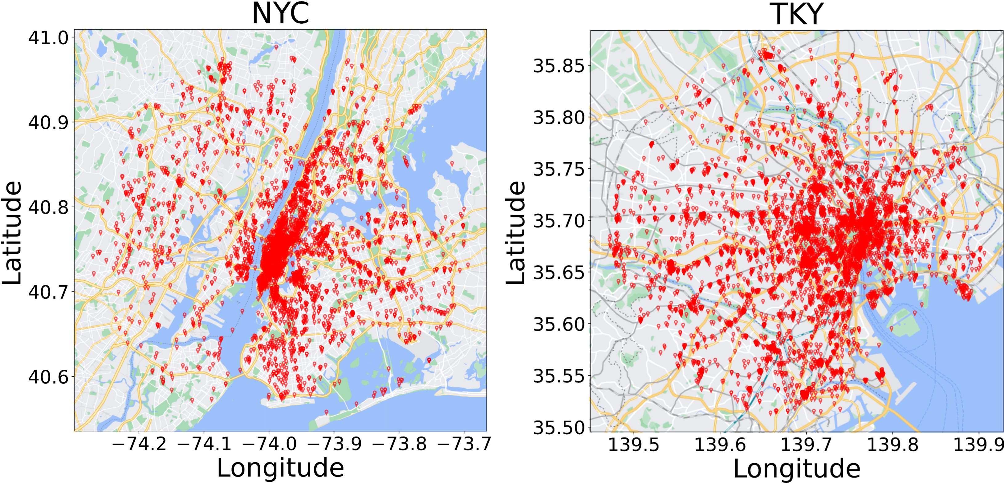
Figure 3: Location distributions of NYC and TKY.

Table II: Main results. NYC & TKY have activity info, different from Foursquare datasets used in some works, there reported results may not directly comparable to this work’s. All experiments here report the best results within a consistent environment.”

Main	NYC						TKY
	R@1	R@5	R@10	N@1	N@5	N@10	R@1	R@5	R@10	N@1	N@5	N@10
Mc	0.189	0.364	0.407	0.189	0.284	0.298	0.170	0.313	0.347	0.170	0.247	0.258
Strnn	0.162	0.255	0.287	0.162	0.213	0.223	0.123	0.209	0.246	0.123	0.169	0.180
DeepMove	0.243	0.387	0.413	0.243	0.322	0.331	0.166	0.268	0.307	0.166	0.221	0.233
Lstpm	0.235	0.436	0.492	0.235	0.342	0.361	0.205	0.366	0.416	0.205	0.292	0.309
Flashback	0.219	0.368	0.423	0.219	0.299	0.317	0.209	0.387	0.447	0.209	0.305	0.325
PG2Net	0.206	0.400	0.430	0.206	0.313	0.323	0.197	0.333	0.376	0.197	0.270	0.284
Plspl	0.187	0.315	0.365	0.187	0.258	0.274	0.166	0.272	0.315	0.166	0.222	0.236
Gcdan	0.188	0.311	0.344	0.188	0.256	0.267	0.171	0.297	0.343	0.171	0.239	0.253
Cslsl*	0.231	0.387	0.421	0.231	0.317	0.328	0.210	0.367	0.417	0.210	0.294	0.310
G-Flashback	0.219	0.371	0.428	0.219	0.300	0.319	0.209	0.387	0.441	0.209	0.304	0.322
Hmt-Grn	0.242	0.406	0.457	0.242	0.333	0.349	0.209	0.371	0.425	0.209	0.295	0.312
Hgarn w/o M, A	0.247	0.406	0.437	0.247	0.335	0.345	0.212	0.371	0.417	0.212	0.299	0.314
Hgarn w/o M	0.264	0.472	0.514	0.264	0.377	0.391	0.228	0.414	0.468	0.228	0.328	0.345
Hgarn w/o A	0.244	0.436	0.486	0.244	0.349	0.365	0.211	0.383	0.438	0.211	0.303	0.321
Hgarn	0.273	0.520	0.575	0.273	0.405	0.423	0.234	0.461	0.526	0.234	0.355	0.376

• The Cslsl paper had label leakage issues, and rerunning the experiment after correction yielded the reported results (This info for reviewers’ reference).

Table III: Comparison of different model sizes.

Strnn	DeepMove	Lstpm	Flashback	PG2Net	Plspl	Gcdan	Cslsl	G-Flashback	Hmt-Grn	Hgarn
75K	4.5M	13M	1.5M	11.8M	15.8M	22.3M	16M	1.5M	50.3M	13.3M

V-B Baselines & Experimental Details

• Mc [4]: Mc is a widely used sequential prediction approach which models transition patterns based on visited locations.

• Strnn [9]: Strnn is an Rnn-based model that incorporates the spatial-temporal contexts by leveraging transition matrices.

• DeepMove [7]: DeepMove uses attention mechanisms and an Rnn module to capture users’ long- and shot-term preferences.

• Lstpm [10]: Lstpm introduces a non-local network and a geo-dilated Lstm to model users’ long- and short-term preferences.

• Flashback [8]: Flashback is an Rnn-based model that leverages spatial and temporal intervals to compute an aggregated hidden state from past hidden states for prediction.

• Plspl [51]: Plspl incorporates activity information to learn user preferences and utilizes two Lstms to capture long-term and short-term preferences.

• PG²Net [52]: PG²Net learns users’ group and personalized preferences with spatial-temporal attention-based Bi-Lstm.

• Gcdan [18]: Gcdan leverages graph convolution to learn spatial-temporal representations and use dual-attention to model the sequential dependencies.

• Cslsl [23]: Cslsl employs multi-task learning to model decision logic and two Rnns to capture long- and short-term preferences.

• Graph-Flashback [20]: Graph-Flashback adds Gcn to Flashback to enrich learned transition graph representations constructed based on defined similarity functions over embeddings from the existing Knowledge Graph Embedding method.

• Hmt-Grn [35]: Hmt-Grn partitions the spatial map and performs a Hierarchical Beam Search to reduce the search space.

To identify the reasons for our Hgarn’s performance improvements, we compare with some variants of Hgarn as follows:

• Hgarn w/o MaHec, Activity: This variant excluded activity input, associated model components and the MaHec label.

• Hgarn w/o MaHec: Hgarn without using the MaHec label.

• Hgarn w/o Activity: This variant removed all activity input and associated model components.

For all baselines and our method, we adopt two commonly-employed metrics in prior works: Rec@K (Recall) and NDCG@K (Normalized Discounted Cumulative Gain). Specific formulas of these two metrics are defined as: $Recall@K=\frac{1}{|U|}\sum_{u\in U}\frac{|l_{u}^{|R_{u}|}\cap\widehat{l_{u,K}^{|R_{u}|}}|}{|l_{u}^{|R_{u}|}|}$ and $NDCG@K=\frac{1}{|U|}\sum_{u\in U}\sum_{i=1}^{K}\frac{|l_{u}^{|R_{u}|}\cap\widehat{l_{u,i}^{|R_{u}|}}|}{\log(i+1)}$, where $\widehat{l^{\cdot}_{u,k}}$ indicates the top $k$ predicted locations.

We port all the baselines to our run time environment for fair comparisons based on their open-source codes. We carefully tuned their hyperparameters to get the best results. Additionally, unlike previous works that only evaluate overall model performances (main setting), we also conduct experiments under the recurring and explorative settings for more comprehensive performance evaluation against the existing SOTAs. For the main and recurring settings, we choose $K=\{1,5,10\}$ for evaluation. As the performance is generally poorer under the explorative setting, we set $K=\{10,20\}$.

For the choice of hyperparameters, we set both $\lambda_{L}$ and $\lambda_{C}$ to 1, $\lambda_{r}$ to 0.6 for both datasets.For embedding dimensions, we set $d=200$, $d^{u}=10$, $d^{t}=30$, $d^{g}=50$ and the dimension of encoders’ hidden states are set to 600. Detailed reproducibility information can be found in supplementary materials.

V-C Main Results

Table II shows the performance comparisons of different methods for the next location prediction. Our Hgarn achieves state-of-the-art performance on both datasets’ metrics. Specifically, Hgarn outperforms the best baseline approach by 12-19% on Recall@$K$ and NDCG@$K$ for NYC and 11-20% for TKY. Its advantages become more significant as $K$ increases, validating the effectiveness of the hierarchical graph modeling and MaHec label for the next location prediction task. We also provide model sizes (i.e., number of model’s trainable parameters) in Table III. Since model sizes are dataset-specific, we use the NYC for demonstration.

Table IV: Performance under the recurring setting.

Recurring	NYC						TKY
	R@1	R@5	R@10	N@1	N@5	N@10	R@1	R@5	R@10	N@1	N@5	N@10
Mc	0.237	0.430	0.474	0.237	0.342	0.357	0.199	0.371	0.408	0.199	0.292	0.304
Strnn	0.189	0.248	0.259	0.189	0.248	0.259	0.162	0.273	0.316	0.162	0.221	0.235
DeepMove	0.243	0.387	0.413	0.243	0.322	0.331	0.209	0.332	0.372	0.209	0.275	0.288
Lstpm	0.282	0.513	0.533	0.282	0.409	0.428	0.249	0.433	0.484	0.249	0.348	0.364
Flashback	0.283	0.507	0.554	0.283	0.406	0.422	0.250	0.462	0.527	0.250	0.363	0.384
PG2Net	0.285	0.492	0.526	0.285	0.398	0.409	0.252	0.411	0.459	0.252	0.338	0.354
Plspl	0.251	0.413	0.450	0.251	0.340	0.352	0.209	0.336	0.384	0.209	0.277	0.292
Gcdan	0.242	0.405	0.439	0.242	0.331	0.342	0.227	0.389	0.436	0.227	0.315	0.330
Cslsl	0.288	0.498	0.542	0.288	0.404	0.418	0.254	0.457	0.511	0.254	0.364	0.382
G-Flashback	0.282	0.509	0.562	0.282	0.406	0.423	0.252	0.463	0.527	0.252	0.364	0.385
Hmt-Grn	0.299	0.514	0.553	0.299	0.417	0.430	0.245	0.446	0.508	0.245	0.352	0.372
Hgarn (our)	0.319	0.633	0.713	0.319	0.487	0.514	0.278	0.552	0.631	0.278	0.424	0.450

In addition, we also evaluate different models separately in the recurring and explorative settings. In the recurring setting, based on results in Table IV, our model shows an improvement of (10.8%, 23.4%, 31.6%, 10.8%, 19.1%, 20.1%) and (9.4%, 19.2%, 19.7%, 9.4%, 16.5%, 16.9%) on all metrics (R@1, R@5, R@10, N@1, N@5, N@10) compared to the best baseline on the two datasets. Hgarn outperforms all baselines significantly in the recurring setting.

Table V: Performance under the explorative setting.

Explorative	NYC				TKY
	R@10	R@20	N@10	N@20	R@10	R@20	N@10	N@20
Strnn	0.066	0.071	0.031	0.033	0.047	0.064	0.021	0.026
DeepMove	0.064	0.112	0.036	0.049	0.04	0.051	0.020	0.031
Lstpm	0.091	0.115	0.052	0.058	0.067	0.090	0.041	0.047
Flashback	0.083	0.109	0.045	0.051	0.053	0.072	0.028	0.032
PG2Net	0.046	0.054	0.021	0.023	0.056	0.065	0.029	0.032
Plspl	0.051	0.061	0.029	0.032	0.056	0.065	0.026	0.032
Gcdan	0.049	0.056	0.025	0.027	0.036	0.048	0.020	0.023
Cslsl	0.078	0.115	0.048	0.057	0.062	0.095	0.030	0.038
Graph-Flashback	0.078	0.104	0.044	0.051	0.053	0.072	0.028	0.032
Hmt-Grn	0.081	0.102	0.052	0.058	0.072	0.098	0.050	0.057
Hgarn (our)	0.102	0.135	0.054	0.062	0.081	0.120	0.037	0.047

As shown in Table V, the overall results in the explorative setting are much lower than those in the main and recurring settings, which is intuitive because of the inherent difficulty of predicting unseen locations. A possible approach to improving the prediction in the explorative setting is to model the dependencies between locations. In addition, due to the larger number of locations in the TKY dataset, the hierarchical graph modeling may introduce noise, making our model less effective in ranking the predicted locations. The above hypotheses may also be why our model performs better in Recall but are not consistently better in NDCG.

V-D Ablation Study

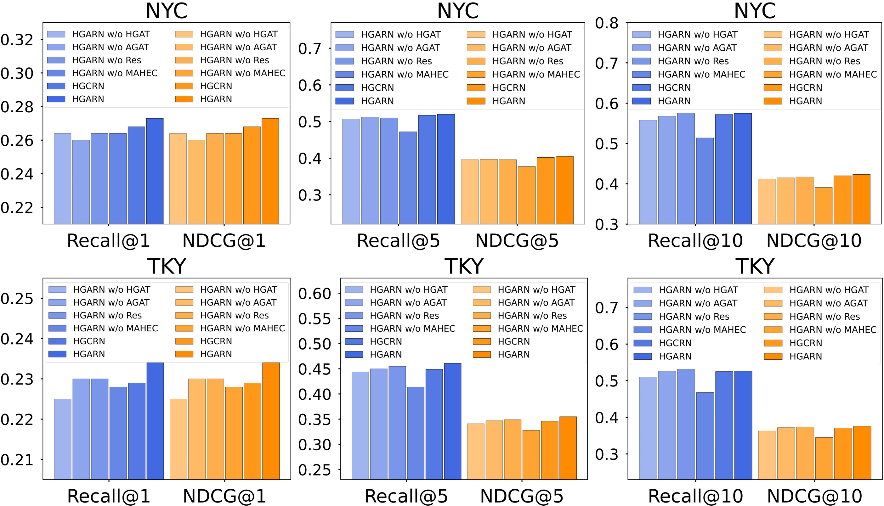
Figure 4: Ablation study results visualization.

To study each component of Hgarn, we conduct an ablation study considering the following four variants of Hgarn: (1) Hgarn w/o HGat contains only the temporal module for next location prediction. (2) Hgarn w/o AGat: This variant’s hierarchical graph attention module contains only the location layer and corresponding graph attention networks. (3) Hgarn w/o Res is the variant that removes the residual connection of the temporal module. (4) Hgarn w/o MaHec is the variant that leverages original labels to optimize our model. (5) Hgcrn is the variant replacing the hierarchical graph attention with hierarchical graph convolution.

V-D1 Discussion for Performance Improvement

The ablation study results are shown in both Table II and Figure 4. In Table II, we found that variant Hgarn w/o M, A could not outperform all baselines, as it omitted activity information and did not utilize MaHec label. By adopting MaHec label, the variant Hgarn w/o Activity performs about (5.3%, 8.1%, 2.8%, 4%) better on metrics (R@5, R@10, N@5, N@10) compared with Hgarn w/o M, A and with no clear improvements on (R@1, N@1), which is consistent with the functionality of MaHec label. By adding activity information, the variant Hgarn w/o MaHec performs about (7.2%, 13.9%, 15.3%, 7.2%, 10.5%, 13.2%) better on metrics (R@1, R@5, R@10, N@1, N@5, N@10) compared with Hgarn w/o M, A, which demonstrates the performance gain by modeling human activities. The full Hgarn achieve best results.

In Figure 4, it is found that all metrics get improved as more components are included. The gradual increase in prediction results from Hgarn w/o HGat to Hgarn w/o AGat to Hgarn is a fine-grained demonstration of the effectiveness of Gat in each layer of the hierarchical graph. In addition, the model’s performance improvements by adding the MaHec label is significant when $K$ are large, verifying its effectiveness under simplicity.

V-D2 Why Attention on the Hierarchical Graph?

Location-based services are likely to be significantly impacted by the ever-changing landscape of locations and functionality. As new stores open or venues close, location-based services must adjust to account for such changes. Graph Attention Networks (Gat) have been shown to outperform Graph Convolutional Networks (Gcn) for graph-based learning tasks by using its self-attention mechanism. This has been supported by Lv et al. [48], who demonstrated that Gat could achieve competitive performance through proper hyperparameter tuning and configuration compared to both homogeneous and heterogeneous Graph Neural Networks. Additionally, Gat provides more robust inductive capabilities that can incorporate newly available (unseen) nodes without retraining. Finally, Gat is more adaptable and scalable than Gcn due to its dynamic scheme that can automatically learn the importance of each node from a graph structure. The hierarchical design can help to overcome the over-smoothing problem [53] of Gnns, the dependencies between location nodes sharing the same activity across regions can be modeled.

V-E Hyperparameter Sensitivity Analysis

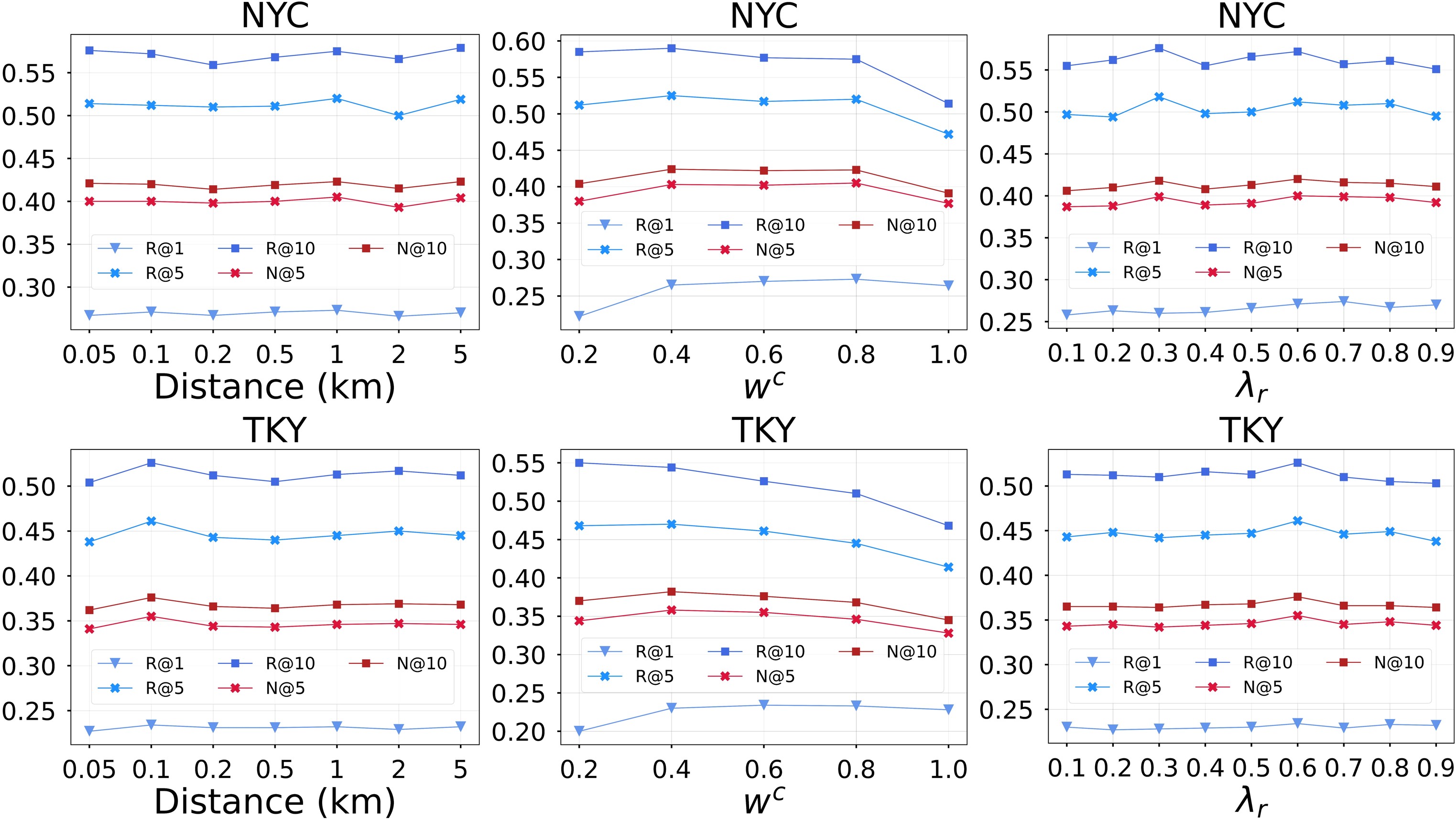
Figure 5: Sensitivity experiments results on two datasets.

We further study the sensitivity of a few key parameters by varying each parameter while keeping others constant. (1) $D^{h}$ affects the location dependencies, too high or too low will lead to decreased performances. The best results were obtained at $D^{h}=1$km on NYC and optimal at $D^{h}=0.1$km on TKY, this is probably because the geographic space and the distance between locations are larger in NYC than in TKY, as in Figure 3. (2) $w^{c}$ A affects the model’s attention to history locations. The results show an upward and then downward trend as $w^{c}$ rises on both datasets, indicating that both too large and too small dependence on locations in the history trajectory is detrimental to the model’s performance. (3) $\lambda_{r}$ affects how much activity information is fused in predicting the next location. Intuitively, a $\lambda_{r}$ too high would introduce noise, and too low may result in ineffective utilization of activity information. The results align with our conjecture that the model achieves optimal performance with $\lambda_{r}$ at 0.6 for both NYC and TKY datasets.

V-F Interpretability Analysis

V-F1 How does MaHec labels work?

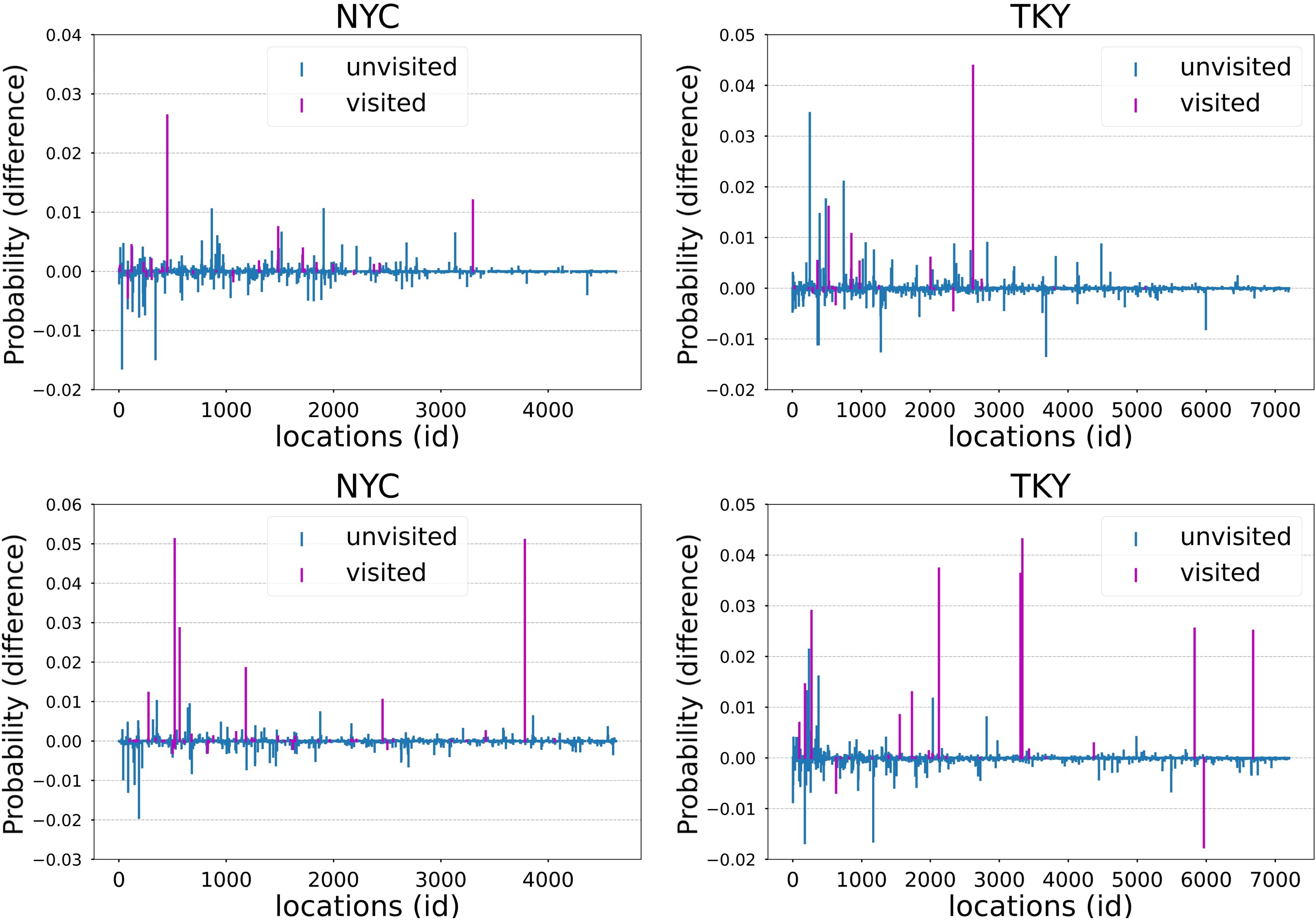
Figure 6: The predicted locations probability distributions difference (with MaHec minus without MaHec).

To understand the mechanism of MaHec label, we randomly selected two human trajectories from two datasets and visualized the predicted probability difference of “Hgarn” and “Hgarn w/o MaHec”. Figure 6 shows the probability change, where the purple line represents the locations in the current user’s history trajectory. With MaHec labels, the probability distribution of the next location predicted by the model increases in most of the visited locations, demonstrating that our MaHec labels can effectively guide the model to pay attention to the user’s history trajectory when predicting the next location. The mechanism of MaHec can also interpret, to some extent, why the prediction performances of our Hgarn can far exceed that of the baseline methods, especially under the recurring setting.

V-F2 What the Hierarchical Graph learned?

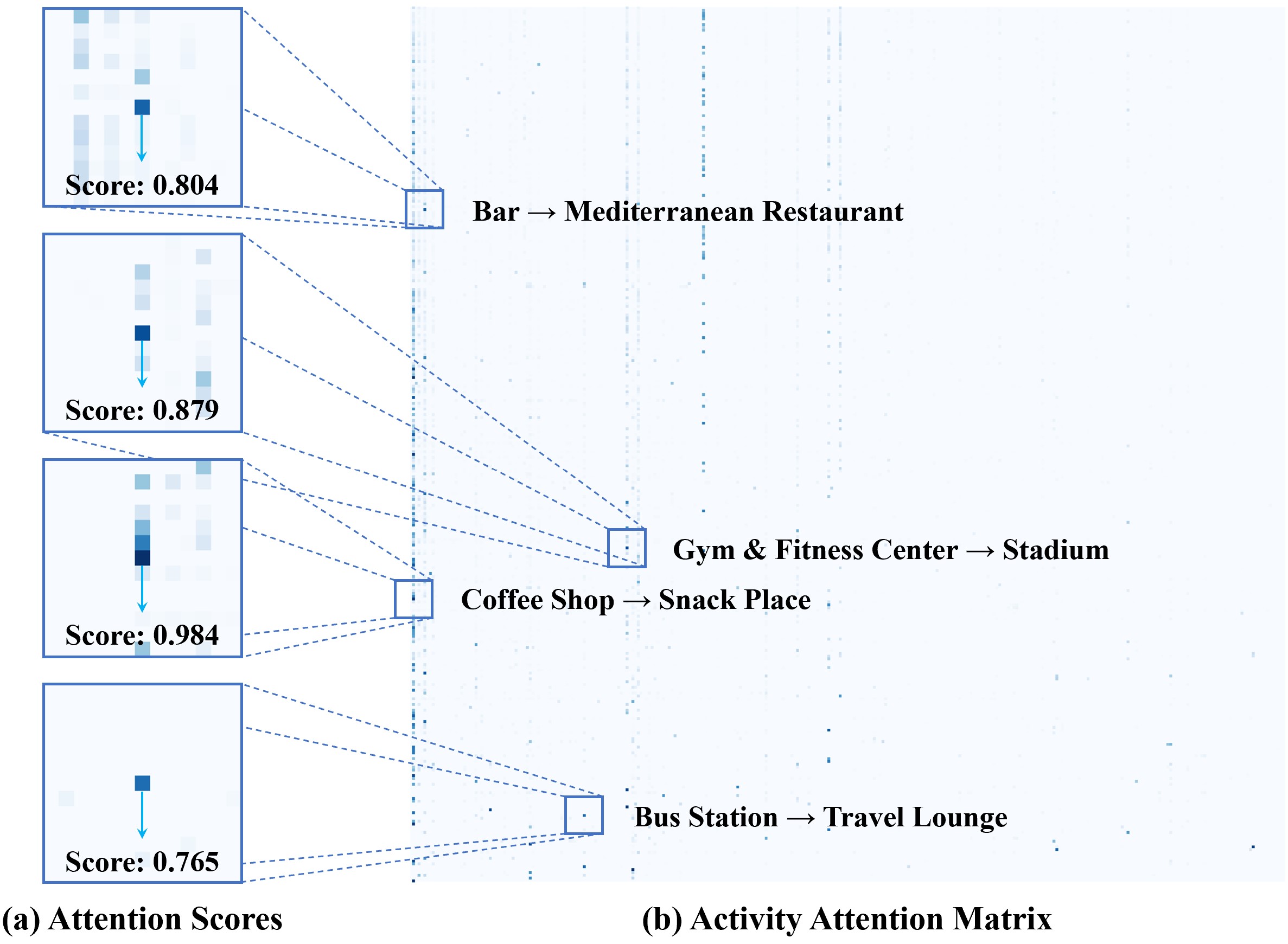
Figure 7: A visualization of activities attentions and cases.

Unlike other methods that have difficulty interpreting learned higher-order spatial-temporal dependencies, our Hgarn can somewhat understand the dependencies between activities through the learned Hierarchical Graph. We visualize one attention head of $\textsc{Gat}_{C}$’s sliced attention matrix to analyze the learned activity-activity dependencies. In Figure 7, We select four activity pairs to show the related activities and their corresponding attention scores. These activity pairs are consistent with common sense human travel, such as the high dependencies between Gyms and Stadiums, Bus Stops and Travel Lounges. These results have important implications for understanding human activity patterns and predicting the next location.

VI Conclusion

Both travel behavior theories and empirical evidence suggest that human mobility patterns largely depend on the need to participate in activities at different times of the day. Therefore, it is crucial to consider the latter when modeling the former. In this paper, we propose a Hierarchical Graph Attention Recurrent Network (Hgarn) for activity-aware human mobility prediction. Specifically, Hgarn introduces hierarchical graph attention mechanisms to model time-activity-location dependencies and uses next activity prediction as an auxiliary task to further improve the main task of next location prediction. In addition, we propose a simple yet powerful MaHec label that can guide our model to flexibly weigh the importance of history locations when predicting future locations. Finally, we perform comprehensive experiments to demonstrate the superiority of Hgarn. To our best knowledge, this is the first work to evaluate different human mobility prediction models (including Hgarn) under recurring and explorative settings. We find that introducing activity information can effectively improve the model’s prediction accuracy. In addition, our results show that the existing models show unsatisfactory prediction performances under the explorative setting. We hope our work could spark the attention of future work on explorative mobility prediction. For future work, we consider a more lightweight design and adding a ranking-based component to organize high-probability candidate locations and incorporate human travel decision logic modeling for better model interpretability.

Yihong Tang received a bachelor’s degree in Computer Science and Technology from the Beijing University of Posts and Telecommunications (BUPT), and he is now a Master of Philosophy (MPhil) student at the Department of Urban Planning and Design, University of Hong Kong (HKU). His research interests include data and graph mining, urban computing, demand and mobility modeling, deep & machine learning systems, recommender systems, and intelligent transportation applications.

Junlin He received a bachelor’s degree in Computer Science and Technology from the Beijing University of Posts and Telecommunications (BUPT), and he is now a Docter of Philosophy (PhD) student at the Department of Civil and Environmental Engineering, The Hong Kong Polytechnic University (PolyU). His research interests include machine learning and intelligent transport systems.

Zhan Zhao is an Assistant Professor in Department of Urban Planning and Design, The University of Hong Kong (HKU), and also affiliated with HKU Musketeers Foundation Institute of Data Science. He holds a Ph.D. degree from the Massachusetts Institute of Technology, a Master’s degree from the University of British Columbia, and a Bachelor’s degree from Tongji University. His research interests include human mobility modeling, public transportation systems, and urban data science.

References

- [1] M. Schläpfer, L. Dong, K. O’Keeffe, P. Santi, M. Szell, H. Salat, S. Anklesaria, M. Vazifeh, C. Ratti, and G. B. West, “The universal visitation law of human mobility,” Nature, vol. 593, no. 7860, pp. 522–527, 2021.
- [2] D. Yang, D. Zhang, V. W. Zheng, and Z. Yu, “Modeling user activity preference by leveraging user spatial temporal characteristics in lbsns,” IEEE Transactions on Systems, Man, and Cybernetics: Systems, vol. 45, no. 1, pp. 129–142, 2014.
- [3] S. Gambs, M.-O. Killijian, and M. N. del Prado Cortez, “Next place prediction using mobility markov chains,” in Proceedings of the first workshop on measurement, privacy, and mobility, 2012, pp. 1–6.
- [4] S. Rendle, C. Freudenthaler, and L. Schmidt-Thieme, “Factorizing personalized markov chains for next-basket recommendation,” in Proceedings of the 19th international conference on World wide web, 2010, pp. 811–820.
- [5] B. Mo, Z. Zhao, H. N. Koutsopoulos, and J. Zhao, “Individual mobility prediction in mass transit systems using smart card data: an interpretable activity-based hidden markov approach,” IEEE Transactions on Intelligent Transportation Systems, 2021.
- [6] S. Hochreiter and J. Schmidhuber, “Long short-term memory,” Neural computation, vol. 9, no. 8, pp. 1735–1780, 1997.
- [7] J. Feng, Y. Li, C. Zhang, F. Sun, F. Meng, A. Guo, and D. Jin, “Deepmove: Predicting human mobility with attentional recurrent networks,” in Proceedings of the 2018 world wide web conference, 2018, pp. 1459–1468.
- [8] D. Yang, B. Fankhauser, P. Rosso, and P. Cudre-Mauroux, “Location prediction over sparse user mobility traces using rnns,” in Proceedings of the Twenty-Ninth International Joint Conference on Artificial Intelligence, 2020, pp. 2184–2190.
- [9] Q. Liu, S. Wu, L. Wang, and T. Tan, “Predicting the next location: A recurrent model with spatial and temporal contexts,” in Thirtieth AAAI conference on artificial intelligence, 2016.
- [10] K. Sun, T. Qian, T. Chen, Y. Liang, Q. V. H. Nguyen, and H. Yin, “Where to go next: Modeling long-and short-term user preferences for point-of-interest recommendation,” in Proceedings of the AAAI Conference on Artificial Intelligence, vol. 34, no. 01, 2020, pp. 214–221.
- [11] A. Vaswani, N. Shazeer, N. Parmar, J. Uszkoreit, L. Jones, A. N. Gomez, Ł. Kaiser, and I. Polosukhin, “Attention is all you need,” Advances in neural information processing systems, vol. 30, 2017.
- [12] Y. Luo, Q. Liu, and Z. Liu, “Stan: Spatio-temporal attention network for next location recommendation,” in Proceedings of the Web Conference 2021, 2021, pp. 2177–2185.
- [13] Q. Guo, Z. Sun, J. Zhang, and Y.-L. Theng, “An attentional recurrent neural network for personalized next location recommendation,” in Proceedings of the AAAI Conference on artificial intelligence, vol. 34, no. 01, 2020, pp. 83–90.
- [14] D. Yang, B. Qu, J. Yang, and P. Cudre-Mauroux, “Revisiting user mobility and social relationships in lbsns: a hypergraph embedding approach,” in The world wide web conference, 2019, pp. 2147–2157.
- [15] B. Chang, G. Jang, S. Kim, and J. Kang, “Learning graph-based geographical latent representation for point-of-interest recommendation,” in Proceedings of the 29th ACM International Conference on Information & Knowledge Management, 2020, pp. 135–144.
- [16] T. N. Kipf and M. Welling, “Semi-supervised classification with graph convolutional networks,” arXiv preprint arXiv:1609.02907, 2016.
- [17] N. Lim, B. Hooi, S.-K. Ng, X. Wang, Y. L. Goh, R. Weng, and J. Varadarajan, “Stp-udgat: spatial-temporal-preference user dimensional graph attention network for next poi recommendation,” in Proceedings of the 29th ACM International Conference on Information & Knowledge Management, 2020, pp. 845–854.
- [18] W. Dang, H. Wang, S. Pan, P. Zhang, C. Zhou, X. Chen, and J. Wang, “Predicting human mobility via graph convolutional dual-attentive networks,” in Proceedings of the Fifteenth ACM International Conference on Web Search and Data Mining, 2022, pp. 192–200.
- [19] H. Wang, Q. Yu, Y. Liu, D. Jin, and Y. Li, “Spatio-temporal urban knowledge graph enabled mobility prediction,” Proceedings of the ACM on Interactive, Mobile, Wearable and Ubiquitous Technologies, vol. 5, no. 4, pp. 1–24, 2021.
- [20] X. Rao, L. Chen, Y. Liu, S. Shang, B. Yao, and P. Han, “Graph-flashback network for next location recommendation,” in Proceedings of the 28th ACM SIGKDD Conference on Knowledge Discovery and Data Mining, 2022, pp. 1463–1471.
- [21] J. Castiglione, M. Bradley, and J. Gliebe, Activity-based travel demand models: a primer, 2015, no. SHRP 2 Report S2-C46-RR-1.
- [22] F. Yu, L. Cui, W. Guo, X. Lu, Q. Li, and H. Lu, “A category-aware deep model for successive poi recommendation on sparse check-in data,” in Proceedings of the web conference 2020, 2020, pp. 1264–1274.
- [23] Z. Huang, S. Xu, M. Wang, H. Wu, Y. Xu, and Y. Jin, “Human mobility prediction with causal and spatial-constrained multi-task network,” arXiv preprint arXiv:2206.05731, 2022.
- [24] J. Chung, C. Gulcehre, K. Cho, and Y. Bengio, “Empirical evaluation of gated recurrent neural networks on sequence modeling,” arXiv preprint arXiv:1412.3555, 2014.
- [25] D. Zhuang, S. Wang, H. Koutsopoulos, and J. Zhao, “Uncertainty quantification of sparse travel demand prediction with spatial-temporal graph neural networks,” in Proceedings of the 28th ACM SIGKDD Conference on Knowledge Discovery and Data Mining, 2022, pp. 4639–4647.
- [26] Z. Zhao, H. N. Koutsopoulos, and J. Zhao, “Individual mobility prediction using transit smart card data,” Transportation Research Part C: Emerging Technologies, vol. 89, pp. 19–34, Apr. 2018.
- [27] C. Cheng, H. Yang, M. R. Lyu, and I. King, “Where you like to go next: Successive point-of-interest recommendation,” in Twenty-Third international joint conference on Artificial Intelligence, 2013.
- [28] J.-D. Zhang, C.-Y. Chow, and Y. Li, “Lore: Exploiting sequential influence for location recommendations,” in Proceedings of the 22nd ACM SIGSPATIAL International Conference on Advances in Geographic Information Systems, 2014, pp. 103–112.
- [29] K. Cho, B. Van Merriënboer, C. Gulcehre, D. Bahdanau, F. Bougares, H. Schwenk, and Y. Bengio, “Learning phrase representations using rnn encoder-decoder for statistical machine translation,” arXiv preprint arXiv:1406.1078, 2014.
- [30] P. Zhao, A. Luo, Y. Liu, F. Zhuang, J. Xu, Z. Li, V. S. Sheng, and X. Zhou, “Where to go next: A spatio-temporal gated network for next poi recommendation,” IEEE Transactions on Knowledge and Data Engineering, 2020.
- [31] R. Li, Y. Shen, and Y. Zhu, “Next point-of-interest recommendation with temporal and multi-level context attention,” in 2018 IEEE International Conference on Data Mining (ICDM). IEEE, 2018, pp. 1110–1115.
- [32] D. Lian, Y. Wu, Y. Ge, X. Xie, and E. Chen, “Geography-aware sequential location recommendation,” in Proceedings of the 26th ACM SIGKDD international conference on knowledge discovery & data mining, 2020, pp. 2009–2019.
- [33] J. Manotumruksa, C. Macdonald, and I. Ounis, “A deep recurrent collaborative filtering framework for venue recommendation,” in Proceedings of the 2017 ACM on Conference on Information and Knowledge Management, 2017, pp. 1429–1438.
- [34] B. Chang, Y. Park, D. Park, S. Kim, and J. Kang, “Content-aware hierarchical point-of-interest embedding model for successive poi recommendation.” in IJCAI, vol. 2018, 2018, p. 27th.
- [35] N. Lim, B. Hooi, S.-K. Ng, Y. L. Goh, R. Weng, and R. Tan, “Hierarchical multi-task graph recurrent network for next poi recommendation,” 2022.
- [36] Y. Yuan, J. Ding, H. Wang, D. Jin, and Y. Li, “Activity trajectory generation via modeling spatiotemporal dynamics,” in Proceedings of the 28th ACM SIGKDD Conference on Knowledge Discovery and Data Mining, 2022, pp. 4752–4762.
- [37] Y. Yuan, H. Wang, J. Ding, D. Jin, and Y. Li, “Learning to simulate daily activities via modeling dynamic human needs,” arXiv preprint arXiv:2302.10897, 2023.
- [38] J. Ho and S. Ermon, “Generative adversarial imitation learning,” Advances in neural information processing systems, vol. 29, 2016.
- [39] J. Bao, Y. Zheng, and M. F. Mokbel, “Location-based and preference-aware recommendation using sparse geo-social networking data,” in Proceedings of the 20th international conference on advances in geographic information systems, 2012, pp. 199–208.
- [40] C. Chen, K. Li, W. Wei, J. T. Zhou, and Z. Zeng, “Hierarchical graph neural networks for few-shot learning,” IEEE Transactions on Circuits and Systems for Video Technology, vol. 32, no. 1, pp. 240–252, 2021.
- [41] L. Mi and Z. Chen, “Hierarchical graph attention network for visual relationship detection,” in Proceedings of the IEEE/CVF conference on computer vision and pattern recognition, 2020, pp. 13 886–13 895.
- [42] D. Liu, X. Qu, X.-Y. Liu, J. Dong, P. Zhou, and Z. Xu, “Jointly cross-and self-modal graph attention network for query-based moment localization,” in Proceedings of the 28th ACM International Conference on Multimedia, 2020, pp. 4070–4078.
- [43] W. Zhang, H. Liu, Y. Liu, J. Zhou, and H. Xiong, “Semi-supervised hierarchical recurrent graph neural network for city-wide parking availability prediction,” in Proceedings of the AAAI Conference on Artificial Intelligence, vol. 34, no. 01, 2020, pp. 1186–1193.
- [44] J. Xu, L. Chen, M. Lv, C. Zhan, S. Chen, and J. Chang, “Highair: A hierarchical graph neural network-based air quality forecasting method,” arXiv preprint arXiv:2101.04264, 2021.
- [45] N. Wu, X. W. Zhao, J. Wang, and D. Pan, “Learning effective road network representation with hierarchical graph neural networks,” in Proceedings of the 26th ACM SIGKDD International Conference on Knowledge Discovery & Data Mining, 2020, pp. 6–14.
- [46] W. Zhang, H. Liu, L. Zha, H. Zhu, J. Liu, D. Dou, and H. Xiong, “Mugrep: A multi-task hierarchical graph representation learning framework for real estate appraisal,” in Proceedings of the 27th ACM SIGKDD Conference on Knowledge Discovery & Data Mining, 2021, pp. 3937–3947.
- [47] Z. Zhou, Y. Liu, J. Ding, D. Jin, and Y. Li, “Hierarchical knowledge graph learning enabled socioeconomic indicator prediction in location-based social network,” Proceedings of WWW 2023, 2023.
- [48] Q. Lv, M. Ding, Q. Liu, Y. Chen, W. Feng, S. He, C. Zhou, J. Jiang, Y. Dong, and J. Tang, “Are we really making much progress? revisiting, benchmarking and refining heterogeneous graph neural networks,” in Proceedings of the 27th ACM SIGKDD Conference on Knowledge Discovery & Data Mining, 2021, pp. 1150–1160.
- [49] P. Veličković, G. Cucurull, A. Casanova, A. Romero, P. Lio, and Y. Bengio, “Graph attention networks,” arXiv preprint arXiv:1710.10903, 2017.
- [50] I. Diaz-Soria, “Being a tourist as a chosen experience in a proximity destination,” Tourism Geographies, vol. 19, no. 1, pp. 96–117, 2017.
- [51] Y. Wu, K. Li, G. Zhao, and Q. Xueming, “Personalized long-and short-term preference learning for next poi recommendation,” IEEE Transactions on Knowledge and Data Engineering, 2020.
- [52] H. Li, B. Wang, F. Xia, X. Zhai, S. Zhu, and Y. Xu, “Pg2net: Personalized and group preferences guided network for next place prediction,” arXiv preprint arXiv:2110.08266, 2021.
- [53] L. Zhao and L. Akoglu, “Pairnorm: Tackling oversmoothing in gnns,” arXiv preprint arXiv:1909.12223, 2019.