Learning Generalizable Models for Vehicle Routing Problems via Knowledge Distillation

Abstract

Recent neural methods for vehicle routing problems always train and test the deep models on the same instance distribution (i.e., uniform). To tackle the consequent cross-distribution generalization concerns, we bring the knowledge distillation to this field and propose an Adaptive Multi-Distribution Knowledge Distillation (AMDKD) scheme for learning more generalizable deep models. Particularly, our AMDKD leverages various knowledge from multiple teachers trained on exemplar distributions to yield a light-weight yet generalist student model. Meanwhile, we equip AMDKD with an adaptive strategy that allows the student to concentrate on difficult distributions, so as to absorb hard-to-master knowledge more effectively. Extensive experimental results show that, compared with the baseline neural methods, our AMDKD is able to achieve competitive results on both unseen in-distribution and out-of-distribution instances, which are either randomly synthesized or adopted from benchmark datasets (i.e., TSPLIB and CVRPLIB). Notably, our AMDKD is generic, and consumes less computational resources for inference.

1 Introduction

The Vehicle Routing Problem (VRP) is a class of NP-hard combinatorial optimization problems with a wide variety of practical applications, such as freight delivery [1], last-mile logistics [2] and ride-hailing [3]. For decades, the problem has been studied intensively in computer science and operations research, with numerous exact and (approximate) heuristic algorithms proposed [4, 5, 6, 7]. Although the heuristic algorithms are usually preferred in practice given their relatively higher computational efficiency, they heavily rely on hand-crafted rules and domain knowledge, which may still leave room for improvement. As a promising alternative, deep (reinforcement) learning could be used to automatically learn a heuristic (or policy) for VRPs in an end-to-end fashion, which has aroused widespread attention in recent years [8, 9, 10, 11, 12, 13, 14, 15, 16]. Compared to the traditional ones, the learned heuristics based on deep models could further reduce computational costs while ensuring desirable solutions.

However, existing deep models suffer from inferior generalization with respect to distributions of node coordinates. To be concrete, they often train and test neural networks on instances of the same distribution, mostly the uniform distribution, where deep models are able to achieve competitive results more efficiently than the traditional heuristics (e.g., [12]). Nevertheless, when the learned policy is applied to infer the out-of-distribution (OoD) instances, the solution quality is usually low. This cross-distribution generalization issue inevitably hinders the applications of deep models, especially because the real-world VRP instances may follow various and even unknown distributions.

A number of preliminary attempts have been made to tackle this generalization issue for VRPs, which mainly leverage (automatic) data augmentation [17, 18, 19, 20] and distributionally robust optimization [21], respectively. However, they are not optimal in our view, as the former always starts with a specified single distribution which may limit the resulted performance, while the latter needs to manually define major and minor instances. Different from them, in this paper, we aim to enhance the cross-distribution generalization by transferring various policies learned from respective distributions into one, where we exploit knowledge distillation to learn more generalizable models for VRPs.

Specifically, we propose a generic Adaptive Multi-Distribution Knowledge Distillation (AMDKD) scheme for training a light-weight model with favorable cross-distribution generalization performance. To impart broad yet specialized knowledge, we exploit multiple teacher models that are (pre-)trained on respective exemplar distributions. Our AMDKD then leverages those teachers to train a shared student model in turns, inspired by the learning paradigm of human-beings. Meanwhile, we also equip the AMDKD with an adaptive strategy to track the real-time learning performance of the student model on every exemplar distribution, which allows the student to concentrate on absorbing those hard-to-master knowledge, so as to strengthen the effectiveness of the learning.

Accordingly, our contributions are summarized as follows: (1) We bring the knowledge distillation to the field of neural combinatorial optimization and aim at improving the cross-distribution generalization for solving VRPs, which offers a promising perspective to transfer knowledge/policy learned from multiple models into one; (2) We propose the Adaptive Multi-Distribution Knowledge Distillation (AMDKD) scheme, where we distill diverse knowledge from multiple teachers trained on exemplar distributions to yield a light-weight yet generalist student model, and also present an adaptive strategy for the student to better assimilate hard-to-master knowledge from difficult distributions; (3) We apply our generic AMDKD to two representative deep models, i.e., AM [10] and POMO [12], respectively. Results show that, while consuming less computational resources for inference, our AMDKD performs favorably against the backbone models as well as other existing generalization methods for deep models, especially on the benchmark dataset CVRPLIB [22]. By further coupling with the efficient active search (EAS) [23], our AMDKD achieves the new state-of-the-art performance. We also conduct a series of analysis to verify our designs.

2 Related work

Recently, neural methods based on deep models for VRPs have aroused widespread interest. These methods are categorized as neural construction models and neural improvement models in general.

Neural construction models. They exploit deep (reinforcement) learning to autoregressively construct the solution in an end-to-end fashion. Vinyals et al. [8] introduced the first RNN-based Pointer Network (Ptr-Net) to solve TSP based on supervised learning. Bello et al. [24] then exploited reinforcement learning to train the Ptr-Net for TSP. In [9], the Ptr-Net was then extended to solve CVRP. Different from the above RNN-based methods, Kool et al. [10] proposed the well-known Attention Model (AM) based on the Transformer architecture [25]. Subsequently, many studies extended AM for routing problems, such as [26, 27, 28, 12, 29, 13, 30]. As a representative, Kwon et al. [12] proposed the POMO (Policy Optimization with Multiple Optima) and achieved significantly better performance. In a recent work, POMO was adapted to an efficient active search (EAS) framework to further boost the performance during inference [23]. Besides, graph neural networks (GNNs) are also utilized to effectively learn and identify the graph-structured features of the problem instance [31, 11, 32, 1, 33].

Neural improvement models. They iteratively improve the initial solution by exploiting deep (reinforcement) learning to assist or control the local search. Chen and Tian [34] proposed the NeuRewriter that learned a policy to partially rewrite the current solution. Hottung and Tierney [35, 36] leveraged deep networks to learn to perform the large neighborhood search. Wu et al. [37] and Costa et al. [38] proposed to control the 2-opt operation [6]. Ma et al. [14] further upgraded the deep model of Wu et al. [37] to dual-aspect collaborative Transformer (DACT) with much superior performance. The DACT method was further enhanced in [39] in order to learn a ruin-and-repair operation for pickup and delivery problems. Generally, improvement methods consume much longer inference time than construction ones to achieve higher solution quality.

Cross-distribution generalization. The above neural methods for VRPs often train and test the deep models on the same instance distribution. Although the state-of-the-art deep models perform close to or even surpass the strong traditional heuristics, they are incapable to generalize the learned policy to other distributions, which seriously impairs their practical applications. Therefore, the cross-distribution issue has gradually gained more attention [17, 18, 19, 20, 21]. Among the early attempts in this line of research, Xin et al. [18] proposed a generative adversarial network (GAN) based framework to generate hard-to-solve instances for training the model. Wang et al. [20] leveraged the game theory and proposed the Policy Space Response Oracle (PSRO) framework to simultaneously learn a trainable solver and an instance generator. Zhang et al. [17] designed a hardness-adaptive TSP instance generator and adopted curriculum learning to train the model. These methods primarily emphasized on data augmentation or are limited to TSP. Different from them, Jiang et al. [21] adopted CNN to acquire distribution-aware features and exploited group DRO (Distributionally Robust Optimization) to enhance model robustness against distributions. However, this method needs to manually define major and minor instances. Note that we acknowledge that the generalization to different problem scales (or sizes) is also important, which we leave as the future research direction.

3 Preliminaries and notations

We first present the formulation of the studied VRPs and classic distributions. Then we introduce how deep models are used to solve them, followed by the basic rationale of knowledge distillation.

3.1 VRPs and their distributions

We define VRPs over a complete graph $\mathcal{G}=\{\mathcal{V},\mathcal{E}\}$, where $v_{i}\in\mathcal{V}$ represents the (customer) node, $e(v_{i},v_{j})\in\mathcal{E}$ represents the edge between two nodes, and $C[e(v_{i},v_{j})]$ represents the cost (we use length in this paper) of the edge. By referring tour $\tau$ (a.k.a. solution) to a permutation of nodes in $\mathcal{V}$, the objective is usually to find the optimal tour $\tau^{*}$ with the least total cost(length) over a finite search space $S$ containing all possible tours, which could be formulated as Eq. (1) in general,

$$\tau^{*}=\mathop{\arg\min}_{\tau^{\prime}\in\mathcal{S}}{L(\tau{{}^{\prime}}|\mathcal{G})}=\mathop{\arg\min}_{\tau^{\prime}\in\mathcal{S}}\sum_{e(v_{i},v_{j})\in\tau^{\prime}}C\left[e(v_{i},v_{j})\right].$$ (1)

For different VRP variants, such objective may be subject to different problem-specific constraints [40, 41], where multiple sub-tours may exist in a valid tour $\tau$. Following the recent literature [10, 12, 23], we focus on two representative VRPs, i.e., TSP and CVRP, respectively. A feasible tour for TSP considers a vehicle visiting each node in $\mathcal{V}$ once and only once. As an extension from a vehicle to a fleet, CVRP considers an extra depot node $v_{0}$ and a capacity limit $Q$ for any given vehicle, where each customer node $v_{i}(i=1,...,n)$ is associated with a demand request $\delta_{i}$. A feasible tour for CVRP consists of multiple sub-tours, each of which represents a vehicle in the fleet departing from the depot, serving a subset of nodes, and finally returning to the depot. The total demand of each sub-tour must not exceed the capacity $Q$, and all nodes except for the depot must be visited once and only once.

Figure 1: VRP instances following various distributions from the literature: (a) gr137, (b) lin105, (c) att532, (d) pr136, (e) X-n125-k30, (f) bier127, (g) Tai150d, (h) Uniform, (i) Cluster, (j) Mixed, (k) Expansion, (l) Implosion, (m) Explosion, (n) Grid, where instances (a)-(g) are from TSPLIB [42] and CVRPLIB [22]. In this paper, we consider instances following distributions (h)-(j) for training and other unseen distributions (k)-(n), as well as unseen benchmark datasets for testing.

In Figure 1, we visualize a number of VRP instances following various distributions from the literature [10, 43, 21], including the TSPLIB [42] and CVRPLIB [22] benchmark datasets. As can be observed, the node coordinates of a VRP instance may follow complicated and even unknown distribution, which considerably intensifies the hardness for solving. While the recent neural methods report superior performance to the traditional heuristics on some fixed distributions, it is unfortunate that they are more sensitive to distribution shift. It is thus of great importance and interest to develop powerful deep models that can simultaneously handle as many diverse distributions as possible.

3.2 Tour construction by deep models

We focus on neural construction methods for VRPs, which usually exploit deep neural networks to sequentially construct the tour. In light of this, the solving procedure is mostly modelled as a Markov Decision Process (MDP), where the Transformer styled [10] architectures following the encoder-decoder structure are often adopted as the policy network. Typically, the encoders project the nodes of the instance into node embeddings for feature extraction. Afterwards, the decoder builds the tour $\tau$ based on learned node embeddings and the partial tour $a_{1:t-1}$ constructed previously. At time step $t$ of the MDP, the decoder picks an unvisited node as the action $a_{t}$ where invalid ones are masked for feasibility. The procedure is repeated until the whole tour is completed, which is factorized as,

$$p_{\theta}(\tau|\mathcal{G})=\prod\limits_{t=1}^{\ell}p_{\theta}(a_{t}|a_{1:t-1},\mathcal{G}),$$ (2)

where $p_{\theta}$ is the policy parameterized by $\theta$, and $\ell$ denotes the final time step in MDP. For TSP, $\ell=n$; for CVRP, $\ell\geq n$ since the depot can be visited more than once. The total reward is defined as the negative of the tour length, i.e., $-L$($\tau|\mathcal{G}$). This is essentially consistent with the objective in Eq. (1).

3.3 Knowledge distillation

Knowledge distillation [44] is a kind of teacher-student training paradigm that aims at transferring knowledge from a (group of) complex teacher model(s) $\theta^{\text{T}}$, to a succinct student model $\theta^{\text{S}}$. The recent research findings reveal that knowledge distillation is not only able to effectively learn a lighter student network from larger teacher network(s) [45, 46], but also has potential to improve the generalization [47, 48] even over its teacher(s) [49, 50, 51]. Typically, the teacher models are pre-trained, and the student model compares the output of teacher model(s) with its own and considers it as a supervisory signal. Formally, the student network is trained with the goal of minimizing a weighted combination of the distillation loss $\mathcal{L}_{\text{KD}}$ and the original task loss $\mathcal{L}_{\text{Task}}$ as follows,

$$\mathcal{L}=\alpha\mathcal{L}_{\text{Task}}+(1-\alpha)\mathcal{L}_{\text{KD}},$$ (3)

where $\alpha\in[0,1]$. The $\mathcal{L}_{\text{KD}}$ with respect to one or more teachers ($N_{T}\!\geq\!1$) is generally formulated as,

$$\mathcal{L}_{\text{KD}}=\frac{1}{N_{T}}\sum\limits_{x\in\mathcal{X}}\sum\limits_{i=1}^{N_{T}}\phi\left[p_{\theta_{i}^{\text{T}}}(x),p_{\theta^{\text{S}}}(x)\right],$$ (4)

where $x$ is the training data from $\mathcal{X}$ and $\phi(\cdot)$ measures the statistical distance between the teacher and the student, such as the Kullback-Leibler divergence $\text{KL}(p_{\theta^{\text{T}}}\|p_{\theta^{\text{S}}})=\sum_{i}p_{\theta^{\text{T}}}(\log p_{\theta^{\text{T}}}-\log p_{\theta^{\text{S}}}$).

4 Methodology

Consider what happens in a classroom when students study multiple modules. Typically, they (students) learn only one module (exemplar distribution) at a time from a professional teacher, and then go on to the next one until all modules are mastered. When students do poorly on a quiz after class (validation dataset), they will be required to study that module more frequently in order to become generalists. Motivated by this, we propose the Adaptive Multi-Distribution Knowledge Distillation (AMDKD) scheme that could efficiently learn more generalizable models for VRPs.

Previously, deep models were trained on a single distribution, e.g., the Uniform in [12, 13, 14]. More recently, attempts have been made to expand the training data by augmenting atypical (minor) [21] or hard instances [18, 17]. Differently, AMDKD allows expert knowledge for tackling distinct distributions to be transferred into a single yet generalist model via distillation. With a light network and high inference speed, the resulted model is supposed to perform favorably against existing methods. Moreover, AMDKD is generic, and could be used to boost various deep models for VRPs.

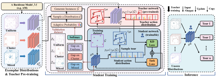
Figure 2: Framework of our AMDKD scheme. From left to right: teacher pre-training, student training and inference. The Uniform is selected as the current exemplar distribution for an example.

4.1 Overall structure and teacher (pre)-training

The overview framework of our AMDKD is illustrated in Figure 2. Given an existing deep model (e.g., AM [10]), AMDKD first performs teacher training (or directly use pre-trained ones) to obtain a teacher model for each distribution listed in a set of exemplar ones. Then in each knowledge transfer epoch, AMDKD picks a specific distribution $d$ and its teacher $\theta^{\text{T}}_{d}$ to train a student network. To facilitate effective learning, the likelihood of picking each distribution is adaptively updated according to the current performance of the student on a validation dataset. Finally, AMDKD performs on-policy distillation, allowing the student network $\theta^{\text{S}}$ to sample RL trajectories (i.e., tours $\{\tau_{\theta^{\text{S}}}\}$) for training, and calculates the two losses (i.e., KD loss and Task loss) for an update.

We consider Uniform, Cluster, and Mixed (mixture of uniform and cluster) as exemplar distributions to train teacher networks in this paper. Consequently, a set of well-trained teachers with parameters $\theta^{\text{T}}=\{\theta^{\text{T}}_{\text{U}},\theta^{\text{T}}_{\text{C}},\theta^{\text{T}}_{\text{M}}\}$ are attained for each distribution. Despite only limited distributions are exploited throughout training, the learned student network is expected to absorb generic and robust knowledge from teachers that may effectively generalize to unseen distributions such as Expansion, Implosion, Explosion, and Grid (visualization in Figure 1). Our motivation here is that each teacher only needs to master a specific distribution, and by working together via our distilling scheme, they can educate a generalist student. Note that the exemplar distributions used here could also be substituted with others (see Section 5.3). Furthermore, since our designed distillation scheme is model-agnostic, the teacher network can follow most of existing architectures. In this paper, we assess our scheme by applying it to two representative construction methods, i.e., AM [10] and POMO [12], respectively.

4.2 Adaptive multi-distribution student training

Given the well-trained teachers on exemplar distributions, our AMDKD student selects one teacher and one distribution in each knowledge transfer epoch and gradually learns to make appropriate decisions. Note that there is another line of works that argue for the simultaneous use of multiple teachers in the distillation process [52, 53]. In their strategy, all teachers are engaged to provide a weighted loss to train the student as aforementioned in Section 3.3. However, such design may require teachers to be trained on a homogeneous task primarily with supervised learning, which does not suit our heterogeneous distributions with reinforcement learning (see Appendix C for results).

Student network. We stipulate that the student shares a similar architecture with its teachers, but can reduce its network parameters as needed to speed up the inference. Nevertheless, we find in Section 5.3 that a larger student model usually leads to a better performance. Therefore, there is a trade-off between solution quality and computational cost. In this paper, we consider reducing the dimension of the node embeddings from $128$ (teacher) to $64$ (student), resulting in a reduction of 61.8% and 59.2% in the model parameters for the adaption with AM and POMO, respectively. We also considered lowering the number of encoder layers, but the results were below the expectation.

The adaptive multi-distribution distilling strategy. In each epoch, AMDKD selects one distribution and its corresponding teacher model. At the beginning, it selects each distribution with an equal probability. After epoch $E^{\prime}$ (a hyper-parameter), the probability would be adaptively adjusted according to the performance of the student on the given validation datasets $\mathcal{Z}_{\text{U}},\mathcal{Z}_{\text{C}},\mathcal{Z}_{\text{M}}$ (each with 1,000 instances) for each exemplar distribution. The likelihood $p^{\text{adaptive}}$ of selecting distribution $d\in\{U,C,M\}$ is proportional to the exponent value of the gaps to the LKH solver [4] as follows,

$$p^{\text{adaptive}}(d)=\left\{\begin{matrix}\text{Softmax}\left({\text{AvgGap}\left[\{\tau_{\theta^{\text{S}}}\}|_{\mathcal{Z}_{d}},\{\tau_{\text{solver}}\}|_{\mathcal{Z}_{d}}\right]}\right),&\text{if }E\geq E^{\prime}\\ \frac{1}{|\mathcal{D}|},&\text{otherwise}\end{matrix}\right.$$ (5)

where $|\mathcal{D}|$ is the number of exemplar distributions; $\{\tau_{\theta^{\text{S}}}\}|_{\mathcal{Z}_{d}}$ and $\{\tau_{\text{solver}}\}|_{\mathcal{Z}_{d}}$ refer to the tour set generated by the student $\theta^{\text{S}}$ and the LKH solver on dataset $\mathcal{Z}_{d}$, respectively. The validation sets are fixed, hence the LKH solver only needs to run once to attain $\{\tau_{\text{solver}}\}|_{\mathcal{Z}_{d}}$ for $d\in\{U,C,M\}$. Meanwhile, we note that $p^{\text{adaptive}}$ may converge during distillation (see Appendix C), which means that it is possible to stop such evaluation early and reuse the stabilized one for an even faster training.

Algorithm 1 Adaptive Multi-Distribution Knowledge Distillation (AMDKD)

0:  A backbone model $\mathcal{M}$ (e.g., AM), exemplar distributions $\mathcal{D}$ (e.g., $\mathcal{D}=\{U,C,M\}$).

1:  Randomly initialize teacher networks $\theta^{\text{T}}_{d}$ ($\forall d\in\mathcal{D}$) and student network $\theta^{\text{S}}$ according to $\mathcal{M}$;

2:  Perform teacher training or leverage pre-train ones (if any) to attain well-learned $\theta^{\text{T}}_{d}$ ($\forall d\in\mathcal{D}$);

3:  for $\text{epoch}=1,2,...,E$ do

4:     Pick distribution $d$ and its teacher $\theta^{\text{T}}_{d}$ with an adaptive probability according to Eq. (5);

5:     for $\text{step}=1,2,...,T$ do

6:         Let student $\theta^{\text{S}}$ sample tours $\tau^{i}_{\theta^{\text{S}}}$ for each $\{\mathcal{G}_{i}\}_{i=1}^{B}$ according to its own policy $p_{\theta^{\text{S}}}$;

7:        Get $\nabla\mathcal{L}_{\text{Task}}$ by estimating Eq. (6) as per the original design of $\mathcal{M}$;

8:        Get $\nabla\mathcal{L}_{\text{KD}}$ by computing the gradients of Eq. (7);

9:        $\theta^{\text{S}}\leftarrow\theta^{\text{S}}+\eta\nabla\mathcal{L}$ where $\nabla\mathcal{L}\leftarrow\alpha\nabla\mathcal{L}_{\text{Task}}+(1-\alpha)\nabla\mathcal{L}_{\text{KD}}$.

10:     end for

11:  end for

Loss function. Following Eq. (3), we leverage the task loss ($\mathcal{L}_{\text{Task}}$) and the KD loss ($\mathcal{L}_{\text{KD}}$) to jointly train the student with $\alpha\!=\!0.5$. Pertaining to $\mathcal{L}_{\text{Task}}$, we define the task loss as follows,

$$\mathcal{L}_{\text{Task}}=-J(\theta^{\text{S}}|d)=-\mathbb{E}_{\mathcal{G}\sim d,\tau\sim p_{\theta^{\text{S}}}(\tau|\mathcal{G})}[L(\tau|\mathcal{G})],$$ (6)

where the training instances $\mathcal{G}$ are sampled following the selected distribution $d$, and the tours $\tau$ are constructed via the student network $\theta^{\text{S}}$ according to Eq. (2). In AM and POMO, the REINFORCE algorithm [54] is used to estimate the gradients for the above loss function and we follow exactly the same way as per their original designs. Pertaining to $\mathcal{L}_{\text{KD}}$, it is defined to encourage the student to imitate how a teacher network sequentially selects the nodes. Specifically, given the instance $\mathcal{G}$ sampled from distribution $d$ and a tour $\tau_{\theta^{\text{S}}}$ constructed by the student $\theta^{\text{S}}$ following its own policy, our AMDKD leverages $p_{\theta^{\text{T}}_{d}}(\tau_{\theta^{\text{S}}}|\mathcal{G})$ suggested by the teacher network $\theta^{\text{T}}_{d}$, to compute $\mathcal{L}_{\text{KD}}$ that measures the similarity of the probability distributions between teacher and student using the KL divergence,

$$\mathcal{L}_{\text{KD}}=\frac{1}{B}\sum_{i=1}^{B}\sum_{a_{j}\in\tau_{\theta^{\text{S}}}}p_{\theta_{d}^{\text{T}}}(a_{j}|\mathcal{G}_{i})\left(\log{p_{\theta_{d}^{\text{T}}}(a_{j}|\mathcal{G}_{i})}-\log{p_{\theta^{\text{S}}}(a_{j}|\mathcal{G}_{i})}\right).$$ (7)

We summarize our AMDKD in Algorithm 1. Note that our AMDKD follows the on-policy scheme where the tours $\tau_{\theta^{\text{S}}}$ are output by the student that currently performs learning. As an alternative, such tours can also be output by the teacher (i.e., off-policy scheme). However, it performs inferior to our on-policy one (see Section 5.3). Finally, we note that the student learned by our AMDKD could also be coupled with the efficient active search (EAS) [23] during inference to further boost the performance. Accordingly, the resulting AMDKD+EAS achieves a new state-of-the-art performance.

5 Experiments

We conduct experiments on TSP and CVRP with $n=$ 20, 50, and 100 nodes similar to [12, 14]. As aforementioned, we adopt Uniform, Cluster and Mixed (mixture of uniform and cluster) as exemplar distributions for training; Expansion, Implosion, Explosion, and Grid as the unseen distributions for testing. For the above 7 distributions, we follow [10, 43, 21] to generate the respective instances (details are presented in Appendix A). All experiments are conducted on a machine with NVIDIA RTX 3090 GPU cards and Intel Xeon Silver 4216 CPU at 2.10GHz. Our implementation in PyTorch are publicly available. Some additional analysis and discussions can be found in Appendix C.

Table 1: Distillation effectiveness of AMDKD on three exemplar distributions.

Model		Size	$n$ = 20				$n$ = 50				$n$ = 100
		(M)	$\text{G}_{\text{U}}$	$\text{G}_{\text{C}}$	$\text{G}_{\text{M}}$	Avg.	$\text{G}_{\text{U}}$	$\text{G}_{\text{C}}$	$\text{G}_{\text{M}}$	Avg.	$\text{G}_{\text{U}}$	$\text{G}_{\text{C}}$	$\text{G}_{\text{M}}$	Avg.
TSP	AM(U)	0.68	0.09%	0.26%	0.19%	0.18%	0.59%	2.24%	1.36%	1.39%	2.10%	7.49%	4.06%	4.55%
	AM(C)	0.68	0.17%	0.10%	0.27%	0.18%	1.41%	0.80%	2.14%	1.45%	3.76%	6.97%	4.39%	5.04%
	AM(M)	0.68	0.15%	0.16%	0.13%	0.15%	1.19%	1.71%	0.87%	1.26%	3.08%	5.65%	2.55%	3.76%
	AMDKD-AM	0.26	0.02%	0.06%	0.05%	0.04%	0.25%	1.64%	0.86%	0.91%	1.21%	5.63%	3.55%	3.46%
	POMO(U)	1.20	0.00%	0.01%	0.01%	0.01%	0.04%	0.42%	0.21%	0.22%	0.17%	1.97%	0.92%	1.02%
	POMO(C)	1.20	0.00%	0.00%	0.01%	0.00%	0.09%	0.07%	0.21%	0.12%	0.41%	0.29%	0.83%	0.51%
	POMO(M)	1.20	0.00%	0.01%	0.00%	0.00%	0.08%	0.17%	0.08%	0.11%	0.77%	1.17%	0.34%	0.76%
	AMDKD-POMO	0.49	0.00%	0.00%	0.00%	0.00%	0.05%	0.05%	0.09%	0.06%	0.34%	0.35%	0.41%	0.37%
CVRP	AM(U)	0.68	1.98%	1.99%	1.98%	1.98%	2.53%	4.33%	2.99%	3.28%	3.10%	9.87%	4.57%	5.85%
	AM(C)	0.68	1.62%	1.43%	1.74%	1.60%	3.08%	2.75%	3.35%	3.06%	4.27%	3.89%	4.93%	4.36%
	AM(M)	0.68	2.09%	2.19%	2.05%	2.11%	2.74%	3.17%	2.31%	2.74%	3.95%	6.26%	3.41%	4.54%
	AMDKD-AM	0.26	0.53%	0.59%	0.64%	0.59%	1.61%	2.66%	1.92%	2.07%	2.08%	5.06%	3.01%	3.38%
	POMO(U)	1.20	0.36%	0.49%	0.51%	0.45%	0.80%	1.53%	1.07%	1.13%	0.95%	2.34%	1.31%	1.53%
	POMO(C)	1.20	0.41%	0.40%	0.54%	0.45%	1.16%	0.93%	1.07%	1.05%	0.93%	1.28%	1.21%	1.14%
	POMO(M)	1.20	0.36%	0.51%	0.40%	0.42%	1.22%	1.34%	0.85%	1.14%	1.89%	2.07%	0.96%	1.64%
	AMDKD-POMO	0.49	0.35%	0.40%	0.41%	0.39%	0.81%	0.97%	0.89%	0.89%	1.06%	1.36%	0.99%	1.13%

• Note: Unless otherwise stated, the gaps are computed w.r.t. the strong traditional solvers Gurobi [5] (for TSP) and LKH [4] (for CVRP).

Training and hyper-parameters. We apply our AMDKD to two representative deep models, i.e., AM [10] and POMO [12], termed as AMDKD-AM and AMDKD-POMO, respectively. For the teacher (pre)-training phase, we directly follow the RL algorithm, network architecture, and other hyper-parameters as suggested in the original backbone method. For the student distillation phase, we use batch size $B$ = 512, and task-specific hyper-parameters $T$ = 250, $E^{\prime}$ = 500 for AMDKD-AM and $T$ = 20, $E^{\prime}$ = 1 for AMDKD-POMO, respectively. By default, the dimension of the node embeddings in our student networks AMDKD-AM and AMDKD-POMO is reduced from 128 (teacher) to 64 (student) to enjoy a faster inference speed. The total numbers of needed training epochs vary with the problem size. Regarding AMDKD-AM, we use 2,000, 5,000, 10,000 for problem sizes 20, 50, 100, respectively (both TSP and CVRP); regarding AMDKD-POMO, we use 5,000 (TSP-20), 10,000 (CVRP-20, TSP-50, TSP-100), and 30,000 (CVRP-50, CVRP-100). The Adam optimizer is used with learning rate 1e-4. Training time also varies with the problem size. Taking CVRP-100 as an example, one epoch takes about 4 minutes for AMDKD-AM and 1.4 minutes for AMDKD-POMO.

Inference. For AMDKD-AM, it samples 1,280 solutions following AM [10]; and for AMDKD-POMO, we adopt the greedy rollout with $\times$8 augments following POMO [12]. All experiments are conducted on test datasets containing 10,000 instances per distribution. Unless otherwise stated, the gaps are computed w.r.t. the strong traditional solvers Gurobi [5] (for TSP) and LKH [4] (for CVRP).

5.1 Effectiveness analysis of AMDKD

We first study the effectiveness of our AMDKD when applied to backbone model AM and POMO for TSP and CVRP, respectively. In Table 1, we display the gaps of the learned student and their respective teachers on unseen instances following three exemplar distributions (denoted as $\text{G}_{\text{U}}$, $\text{G}_{\text{C}}$, and $\text{G}_{\text{M}}$) and also report the parameter sizes of each model. We can see that when the teacher model is trained on a specific distribution, it does not generalize well on the other ones (especially for AM), resulting in poor overall performance (if referring to the average gaps). In contrast, our AMDKD could alleviate this issue effectively. While the learned student model by AMDKD reduces the size of the teacher model from 0.68 to 0.26 M (a 61.8% reduction) for AM and from 1.20 to 0.49 M (a 59.2% reduction) for POMO, it still exhibits improved overall performance for both TSP and CVRP on all the three sizes. Pertaining to AMDKD-AM, our AMDKD student not only significantly outperforms its three teachers for both TSP and CVRP, but also exhibits even lower gaps on the distribution where the teacher was previously trained in most cases. Pertaining to AMDKD-POMO, although POMO itself presents a better generalization, our AMDKD can still boost its overall performance with a much lighter student network for both TSP and CVRP. The above results validate that our AMDKD does not overfit to a single distribution, and successfully learns a lightweight yet generalist student model under the guidance of multiple teachers with expertise in different exemplar distributions.

5.2 Generalization analysis of AMDKD

We now assess the cross-distribution generalization of our AMDKD. In addition to the two backbone models, we also compare with the following methods, i.e., 1) other deep models including- 1.a) DACT [14], a neural improvement model that learns to perform local search; 1.b) LCP [13] (TSP only), a hybrid two-stage method that combines improvement and construction strategy; and 2) other methods specialized for generalization including- 2.a) HAC [17] (TSP only), a fine-tuning framework for AM by leveraging instances with different hardness; 2.b) DROP [21], a distributionally robust optimization based method to enhance POMO; 2.c) GANCO [18], a framework that enhances AM by learning a generative adversarial network to produce hard-to-solve training instances; and 2.d) PSRO (a.k.a. LIH) [20], an improvement method with a game theory based policy space response oracle framework. More implementation details of them are provided in Appendix B. Note that for DROP, GANCO, and PSRO, we only compare the results on several benchmark instances reported in their original papers (see Table 3), since their codes (for re-training) are not publicly available.

Table 2: Generalization on unseen in-distribution (ID) and out-of-distribution (OoD) instances.

Model		Size	$n=$ 20			$n=$ 50			$n=$ 100
		(M)	$\text{G}_{\text{ID}}$	$\text{G}_{\text{OoD}}$	Time∗	$\text{G}_{\text{ID}}$	$\text{G}_{\text{OoD}}$	Time∗	$\text{G}_{\text{ID}}$	$\text{G}_{\text{OoD}}$	Time∗
TSP	Gurobi	-	-	-	0.01s (7s)	-	-	0.08s (51s)	-	-	0.7s (7.6m)
	HAC#	0.68	0.11%	0.07%	0.03s (48s)	1.05%	0.57%	0.09s (4m)	4.68%	2.97%	0.19s (16m)
	LCP#	2.03	0.11%	0.03%	1.2s (43m)	6.70%	0.99%	1.5s (2.8h)	32.70%	8.24%	2.4s (6.4h)
	DACT(T=1,280)#	0.27	0.11%	0.08%	12s (2.1m)	0.31%	0.34%	19s (7.2m)	2.37%	3.13%	28s (23m)
	AM# (128)	0.68	0.18%	0.10%	0.03s (48s)	1.48%	0.74%	0.09s (4m)	4.15%	2.84%	0.19s (16m)
	AM# (64)	0.26	0.21%	0.11%	0.03s (35s)	1.74%	0.83%	0.08s (2.8m)	5.93%	3.85%	0.17s (11m)
	AMDKD-AM (64)	0.26	0.04%	0.02%	0.03s (35s)	0.91%	0.37%	0.08s (2.8m)	3.46%	1.87%	0.17s (11m)
	POMO# (128)	1.20	0.00%	0.00%	0.03s (5s)	0.07%	0.05%	0.09s (16s)	0.30%	0.28%	0.13s (1.1m)
	POMO# (64)	0.49	0.02%	0.01%	0.02s (4s)	0.18%	0.16%	0.04s (11s)	0.69%	0.59%	0.12s (50s)
	AMDKD-POMO (64)	0.49	0.00%	0.00%	0.02s (4s)	0.06%	0.05%	0.04s (11s)	0.37%	0.41%	0.12s (50s)
	AMDKD+EAS†	0.49	0.00%	0.00%	5s (4.5m)	0.01%	0.01%	12s (28m)	0.11%	0.10%	28s (2.3h)
CVRP	LKH3	-	-	-	7.7s (1.3h)	-	-	31s (5.3h)	-	-	56s (9.6h)
	DACT(T=1,280)#	0.27	0.09%	0.05%	28s (4.3m)	1.59%	1.59%	55s (14m)	5.56%	5.55%	1.5m (34m)
	AM# (128)	0.68	2.00%	1.98%	0.05s (1.2m)	3.39%	2.66%	0.12s (5m)	5.42%	3.75%	0.26s (18m)
	AM# (64)	0.26	2.02%	2.02%	0.05s (49s)	3.62%	2.65%	0.11s (3.6m)	6.83%	4.56%	0.23s (13m)
	AMDKD-AM (64)	0.26	0.59%	0.55%	0.05s (49s)	2.07%	1.69%	0.11s (3.6m)	3.38%	2.44%	0.23s (13m)
	POMO# (128)	1.20	0.42%	0.39%	0.05s (7.8s)	0.92%	0.94%	0.10s (18s)	1.14%	1.21%	0.19s (1.3m)
	POMO# (64)	0.49	0.55%	0.51%	0.05s (6.1s)	1.19%	1.21%	0.08s (15s)	1.43%	1.50%	0.18s (1.1m)
	AMDKD-POMO (64)	0.49	0.39%	0.36%	0.05s (6.1s)	0.89%	0.90%	0.08s (15s)	1.13%	1.21%	0.18s (1.1m)
	AMDKD+EAS†	0.49	-0.04%	-0.06%	9s (7.8m)	0.07%	0.04%	20s (37m)	-0.03%	-0.04%	40s (3.3h)

• We report the average time to solve one instance, and the total time to solve 10,000 instances in ($\cdot$) with batch parallelism allowed (one GPU).

• The corresponding model is trained on a mixed training dataset that contains instances from all the three exemplar distributions.

• For EAS, we adopt its EAS-lay version (T=100) for demonstration purpose.

Distribution mixture augmentation. Given that baselines AM, POMO, DACT, and LCP were originally trained on the uniform distribution only (resulting in poor generalization), we re-train the above models (with ^#) on a mixed dataset containing instances from the three exemplar distributions, to ensure a fair comparison. We also apply this mixed dataset as the initial training instances for HAC (with ^#). Though such distribution mixture augmentation improves the generalization of construction methods POMO and AM on larger instances, we notice that it does not always happen so, especially for the methods that have an improvement component (e.g., DACT and LCP). We present detailed results and discussions regarding this finding in Appendix B. Meanwhile, for AM^# and POMO^#, we report their performance with network dimensions of both 128 and 64 (same size as our AMDKD student) for a more comprehensive comparison. We assess the following metrics, 1) parameter size; 2) average gap on unseen in-distribution instances, i.e., $\text{G}_{\text{ID}}$; 3) average gap on unseen out-of-distribution instances, i.e., $\text{G}_{\text{OoD}}$; 4) average time for solving an individual instance and total time for solving 10,000 instances with batch parallelism allowed (one GPU).

As can be observed in Table 2, our AMDKD is able to achieve competitive results on both unseen in-distribution and out-of-distribution instances, and performs favourably against all baselines. Pertaining to TSP, our AMDKD-AM (64) significantly outperforms the baseline AM^# (128) and AM^# (64) on all sizes in terms of both $\text{G}_{\text{ID}}$ and $\text{G}_{\text{OoD}}$ with fewer parameters and higher inference speed. Meanwhile, it also consistently beats the recent baseline HAC^# (designed to boost the generalization of AM) on all sizes in terms of both two gaps and the time efficiency. For the backbone model POMO, which suffers from less generalization concern, the baseline POMO^# (128) can already attain near-optimal solutions to TSP instances with a desirable generalization performance. However, our AMDKD (64) is able to achieve competitive generalization results with nearly half of the model size and higher inference speed. When we reduce the network dimension of POMO^# to 64 (as our AMDKD), POMO^# (64) performs much inferior to our AMDKD-POMO (64). Pertaining to CVRP, similar patterns can be observed, where our AMDKD-AM (64) and AMDKD-POMO (64) consistently deliver favourable generalization performance against all the compared baselines. Besides, both our AMDKD-AM (64) and AMDKD-POMO (64) exhibit significantly faster inference than improvement methods LCP and DACT while achieving similar or even lower gaps.

Furthermore, we show that by coupling our AMDKD-POMO (64) model with the recent efficient active search (EAS) [23], the resulting AMDKD+EAS (T=100) attains considerably superior performance that even surpasses LKH3 on CVRP-100 with much shorter time. Given the advances of active search for a particular instance to be inferred, AMDKD+EAS allows the model learned by our AMDKD with strong generalization to continuously improve its performance during inference (longer T will yield even better performance), which leads to a new state-of-the-art hybrid solver.

We now evaluate the generalization of our AMDKD on the benchmark, i.e., TSPLIB and CVRPLIB, which contain various instances of unknown distributions and larger size. As shown in Table 3, our AMDKD-AM (64) significantly boosts the generalization of AM (128) and also outperforms the baseline AM^# (128) as well as other generalization methods that take AM (128) as the backbone model (GANCO and HAC). Similarly, our AMDKD-POMO (64) also significantly beats the other baseline methods, except for POMO^# (128) on TSPLIB. Nevertheless, regarding the harder CVRP instances from CVRPLIB, our AMDKD-POMO (64) could yield significantly better performance. Finally, we note that the AMDKD+EAS achieves the smallest gaps for both TSP and CVRP among all baselines. We refer to Appendix D for full results and discussions.

Table 3: Generalization performance on selected instances (100 $\!\leq\!n\!\leq\!$ 200) from benchmark datasets.

	PSRO	AM (128)	GANCO	HAC	AM${}^{\#}(128)$	AMDKD-AM (64)	POMO (128)	DROP	POMO${}^{\#}(128)$	AMDKD-POMO (64)	AMDKD+EAS
TSPLIB	4.47%	42.63%	4.87%	6.06%	17.60%	3.53%	29.73%	10.79%	0.87%	1.08%	0.74%
CVRPLIB	-	29.36%	-	-	13.88%	7.43%	14.19%	8.67%	6.80%	4.38%	1.26%

5.3 Further analysis of AMDKD

Effects of different components. We conduct ablation studies on CVRP-50 and TSP-50 to verify the designs of our AMDKD, where we consider removing the proposed adaptive strategy, the KD loss $\mathcal{L}_{\text{KD}}$, and the task loss $\mathcal{L}_{\text{Task}}$, respectively. As displayed in Table 4, the use of adaptive strategy further enhances the learning effectiveness, and the two losses play a prominent role in the phase of gradient update. We also verify that when compared with our on-policy scheme, the off-policy variant (as mentioned in Section 4.2) saliently impairs the distillation performance.

Table 4: Ablation studies of AMDKD designs.

Model	Components				CVRP-50	TSP-50
	$p^{\text{adaptive}}$	$\mathcal{L}_{\text{KD}}$	$\mathcal{L}_{\text{Task}}$	$\tau_{\theta^{\text{S}}}$	Avg. Gap	Avg. Gap
w/o adaptive		✓	✓	✓	0.94%	0.69‰
w/o $\mathcal{L}_{\text{KD}}$	✓		✓	✓	1.06%	0.66‰
w/o $\mathcal{L}_{\text{Task}}$	✓	✓		✓	1.00%	0.69‰
off-policy	✓	✓	✓		10.42%	0.80‰
AMDKD	✓	✓	✓	✓	0.90%	0.63‰

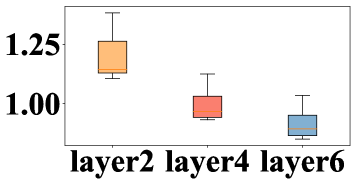
(a)

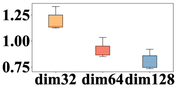
(b)

Figure 3: Effects of student network architectures. (a) different numbers of encoder layers, (b) different node embedding dimensions.

Effects of student network architectures. In Figure 3, we exhibit the boxplots of the averaged gaps when using different student network architectures (different dimensions of the entire network and different number of layers in its encoder) of AMDKD-POMO for solving CVRP-50. As revealed, the larger the model, the better its performance. Hence, we acknowledge that our AMDKD can be further boosted when the student (64) shares the same architecture with its teachers (128). Specifically, for CVRP-50, our AMDKD-POMO (128) exhibits an average optimality gap of 0.81%, which is lower than the 0.90% of AMDKD-POMO (64). However, this improvement comes at the expense of increased computational costs in three aspects: 1) more training time - AMDKD-POMO (128) needs almost 1.7 times (12 days vs 7 days) more training time; 2) more parameters - AMDKD-POMO (128) has about 2.4 times (1.20 M vs 0.49 M) more parameters; 3) slower inference time - AMDKD-POMO (128) infers about 1.2 times (1.3 min vs 1.1 min) slower than AMDKD-POMO (64). Hence, we note that there is a trade-off between solution quality and computational cost.

Effects of different exemplar distributions. We now vary the distributions which were used as the exemplar ones to validate that AMDKD could still be effective. We take the POMO and CVRP-50 as an example. To distinguish from the original version (AMDKD-POMO), we term the model taking Expansion, Implosion, Explosion, and Grid as the exemplar distributions as AMDKD-POMO*, and gathered the results in Table 5. It shows that the overall performance of AMDKD-POMO* is still better than POMO trained on these four distributions respectively. Hence, our AMDKD is able to consistently improve the cross-distribution generalization with different exemplar distributions.

Table 5: Performance of AMDKD on CVRP-50 trained with different exemplar distributions.

Model	Size	Expansion		Implosion		Explosion		Grid		Uniform		Cluster		Mixed		Avg. Gap
	(M)	Obj.	Gap	Obj.	Gap	Obj.	Gap	Obj.	Gap	Obj.	Gap	Obj.	Gap	Obj.	Gap
LKH3	-	8.15	-	10.26	-	8.74	-	10.40	-	10.38	-	5.13	-	9.42	-	-
POMO(Expansion)	1.20	8.22	0.90%	10.36	0.96%	8.82	0.94%	10.50	0.95%	10.47	0.94%	5.19	1.14%	9.51	0.96%	0.97%
POMO(Implosion)	1.20	8.23	0.96%	10.34	0.80%	8.81	0.82%	10.48	0.77%	10.46	0.78%	5.21	1.50%	9.52	1.03%	0.95%
POMO(Explosion)	1.20	8.23	0.95%	10.35	0.83%	8.81	0.80%	10.49	0.82%	10.47	0.87%	5.20	1.27%	9.51	1.02%	0.94%
POMO(Grid)	1.20	8.23	0.97%	10.34	0.79%	8.81	0.82%	10.48	0.76%	10.46	0.77%	5.21	1.57%	9.52	1.07%	0.97%
AMDKD-POMO*	0.49	8.23	0.96%	10.35	0.89%	8.82	0.89%	10.49	0.88%	10.47	0.88%	5.18	1.06%	9.50	0.92%	0.92%

6 Conclusions and future work

In this paper, we propose an Adaptive Multi-Distribution Knowledge Distillation (AMDKD) scheme to alleviate the cross-distribution generalization issue of deep models for VRPs. Different from the existing generalization methods, we aim to enhance the distribution generalization by transferring various policies learned from exemplar distributions into one via an efficient knowledge distillation scheme. To facilitate effective learning, we design an adaptive strategy to train a single yet generalist student network by leveraging multiple teachers in turns. The experiment results exhibit competitive performance of our AMDKD in generalizing to other unseen out-of-distribution instances (randomly generated or from benchmarks), which also consumes less computational resources. While our AMDKD is generic, a potential limitation is that its boost is not guaranteed to be always significant across all unseen distributions for all backbone models. For future work, we will investigate, 1) generalizing AMDKD for different/larger problem sizes; 2) considering the improvement models like DACT [14] as the backbone; 3) performing online distillation to jointly and efficiently train the teachers and the student models [55]; 4) assessing the impact of the quality of the validation dataset on the distillation; and 5) enhancing the interpretability of AMDKD [56].

 
Learning Generalizable Models for Vehicle Routing Problems via Knowledge Distillation (Appendix)
 

Appendix A Details of the considered distributions

In this paper, we consider various distributions for the node coordinates in VRPs, followed which we randomly generate instances for both training and testing. Below we present details on how to generate those instances. Specifically, we follow the recent work [10] and benchmark dataset TSPLIB [42] to generate instances of Uniform, Cluster and Mixed distributions, and follow the settings in [21, 43] for the Expansion, Implosion, Explosion, and Grid ones.

Uniform distribution. It considers uniformly distributed nodes. Following [10], we generate the two-dimensional coordinates $(x,y)$ of each node by sampling from a uniform space $\mathcal{U}$([0, 1]²). An exemplary instance is displayed in Figure 1(h).

Cluster distribution. It considers multiple ($n_{c}$) clusters, where we set $n_{c}=3$. In specific, each cluster follows a normal distribution $\mathcal{N}$($\mu$, $\sigma^{2}$)² with the mean sampled uniformly, i.e., $\mu\sim\mathcal{U}$([0.2, 0.8]²) and the standard deviation $\sigma$ = 0.07. According to the 3$\sigma$ rule, each node has a 99.7% probability of being generated in the [0, 1]² square region, and outliers will have their coordinates re-modified, where values less than 0 are changed to 0 and those greater than 1 are changed to 1, to ensure all coordinates are constrained to ([0, 1]²). An exemplary instance is displayed in Figure 1(i).

Mixed distribution. It considers a mixture of the two distributions above, each with half of the nodes. For the latter, we only consider $n_{c}\!=\!1$ cluster. An exemplary instance is displayed in Figure 1(j).

Expansion distribution. It considers a linear function to mutate the nodes in Uniform distribution. Gvien a randomly generated linear function $y=ax+b$, all nodes, orthogonal to the linear function within the distance $r$ ($r=0.3$), are moved away from their original coordinates to a farther position, whose orthogonal distance is $r+\gamma$, where $\gamma$ obeys an exponential distribution with the rate parameter $\lambda=10$, i.e. $\gamma\sim E(\lambda)$. Regarding the linear function, we first sample $b$ (intercept) from [0, 1], then $a$ (slope) is sampled uniformly from [0, 3] (if $b$ < 0.5) or [-3, 0] (if $b\geq$ 0.5). Finally, we normalize all node coordinates $X$ as follows to ensure that they are constrained to [0, 1]²,

$$X^{\prime}=\frac{X-\text{min}(X)}{\text{max}(X)-\text{min}(X)},$$ (8)

where $X^{\prime}$ denotes the normalized coordinates. An exemplary instance is displayed in Figure 1(k).

Implosion distribution. It considers an implosion to mutate the nodes in Uniform distribution. To simulate an implosion, it first samples a centroid $\epsilon_{\text{i}}$, then gathers all nodes within the circle of $\epsilon_{\text{i}}$ (with the radius $R_{\text{ic}}=0.3$) together towards a new circle with the same centroid $\epsilon_{\text{i}}$ but a (randomly sampled) smaller radius ($R_{\text{i}}\leq 0.3$). An exemplary instance is displayed in Figure 1(l).

Explosion distribution. It considers to mutate the nodes in Uniform distribution by imitating the particles affected by an explosion. Similar to Implosion, it first randomly samples a centroid. Then, instead of gathering all nodes towards the centroid in Implosion distribution, it moves away those nodes from the circle (radius $R_{\text{ec}}\!=\!0.3$) and explode them outside the circle, which follow the direction vector between the centroid $\epsilon_{\text{e}}$ and the corresponding nodes. The additive distance $\gamma$ is randomly sampled from an exponential distribution with a rate parameter, i.e. $\gamma\sim E(\lambda)$. All nodes are them normalized using Eq. (8). An exemplary instance is displayed in Figure 1(m).

Grid distribution. It considers to mutate the nodes in Uniform distribution by imposing a grid permutation. We first generate the four vertex of a square with the width and height equal to $R_{\text{g}}(R_{\text{g}}=0.3)$ and then place it within the region [0, 1]². All the pre-generated nodes inside the box are re-arranged as a quadratic grid instead. In this case, all nodes are constrained to [0, 1]². An exemplary instance is displayed in Figure 1(n).

The above distributions are considered in both TSP and CVRP. For extra settings in CVRP, we follow the convention [10, 14, 12]. In specific, the demand $\delta_{i}$ of each node is sampled uniformly from $\mathcal{U}$(1, 2, $\cdots$, 9) and the capacity $Q$ of the vehicle varies with the problem scale, where we set $Q^{20}$ = 30, $Q^{50}$ = 40 and $Q^{100}$ = 50. For instances from CVRPLIB, we exactly follow their settings.

Appendix B Details of compared baselines

Implementation Details. We compare our AMDKD with various types of baselines. Regarding the neural baselines, we re-train LCP [13], HAC [17] and DACT [14] on our machine based on the code that are publicly available on Github. By default, we follow their original settings and the suggestion on the hyper-parameters. More details of the baselines are presented below.

• Gurobi [5]: we use Gurobi to obtain the optimal solutions to TSP instances, which are implemented under the default settings.

• LKH [4]: For CVRP, it is usually hard to obtain the optimal solutions. Thus, we use the strong LKH solver to find near-optimal solutions. Note that the LKH solver is also a widely used baseline to evaluate and compare the recent learning based methods for VRPs, where we run it following the conventions in [10, 14, 12, 23].

• LCP [13]: LCP is a two-stage method, where a seeder generates diverse initial solutions and a reviser rewrites the current solutions partially. We re-train the LCP on a mixed dataset containing instances from the three exemplar distributions. For inference of TSP-50 and TSP-100, we employ the LCP* (the best version reported in [13]) with two revisers (the lengths of the tour for revision are set to $\ell_{r1}$=10 and $\ell_{r2}$=20) and a sampling strategy (1,280), and set the total number of revision iteration $T_{r}$ to 45 (i.e., $T_{r1}$=25, $T_{r2}$=20, respectively). For TSP-20, we exploit one reviser ($\ell_{r}$=10) since the revision length must be less than the problem size according to its design, and set the number of revision iteration $T_{r}$ to 10.

• HAC [17]: HAC designs a hardness-adaptive Gaussian instances generator to produce instances to fine-tune the given pre-trained AM model. In its original design, the dataset used for fine-tuning contains half instances uniformly distributed and the other half produced by its own generator. In this paper, we substitute the instances of uniform distribution with a mixed dataset containing instances from the three exemplar distributions.

• DACT [14]: DACT learns to guide the pairwise operator to perform local search. We adopt the 2-opt version since it reports the best result for TSP and CVRP according to its original paper [14]. We re-train DACT on a mixed dataset containing instances from the three exemplar distributions, and set the iteration number to 1,280 for inference.

Table 6: Effects of distribution mixture during training.

Model		$n$ = 50								$n$ = 100
		Uniform	Cluster	Mixed	Grid	Implosion	Expansion	Explosion	Avg.	Uniform	Cluster	Mixed	Grid	Implosion	Expansion	Explosion	Avg.
TSP	Gurobi	5.70	2.65	4.92	5.69	5.60	4.38	4.62	-	7.76	3.66	6.73	7.79	7.61	5.39	5.83	-
	POMO (U)	5.70	2.66	4.93	5.69	5.60	4.38	4.62	0.12%	7.78	3.73	6.79	7.8	7.62	5.43	5.85	0.61%
	POMO#	5.70	2.66	4.93	5.69	5.60	4.38	4.62	0.06%	7.78	3.67	6.75	7.81	7.63	5.42	5.84	0.29%
	AM (U)	5.73	2.71	4.99	5.73	5.63	4.43	4.65	1.02%	7.93	3.93	7.00	7.95	7.78	5.64	5.98	3.58%
	AM#	5.73	2.72	4.99	5.73	5.64	4.43	4.65	1.06%	7.92	3.90	7.00	7.95	7.77	5.66	5.98	3.40%
	LCP (U)	5.72	3.58	5.01	5.71	5.62	4.44	4.65	5.70%	7.95	6.91	7.34	7.98	7.81	6.23	6.26	18.31%
	LCP #	5.73	3.11	5.04	5.72	5.63	4.47	4.65	3.44%	7.99	6.81	7.34	8.02	7.85	6.41	6.30	18.72%
	HAC (U)	5.81	2.87	5.07	5.80	5.71	4.48	4.70	3.00%	8.14	4.24	7.26	8.17	7.99	5.96	6.16	7.78%
	HAC#	5.72	2.70	4.97	5.72	5.63	4.41	4.64	0.78%	7.96	3.94	6.98	7.98	7.81	5.60	6.01	3.70%
	DACT (U)	5.70	2.69	4.98	5.70	5.61	4.43	4.63	0.61%	7.90	3.90	6.98	7.92	7.75	5.80	5.99	3.67%
	DACT#	5.71	2.66	4.94	5.71	5.62	4.40	4.63	0.33%	7.96	3.74	6.88	7.98	7.80	5.67	5.98	2.80%
CVRP	LKH3	10.38	5.13	9.42	10.40	10.26	8.15	8.74	-	15.65	7.81	14.19	15.64	15.44	11.39	12.32	-
	POMO (U)	10.46	5.21	9.52	10.49	10.35	8.23	8.81	0.98%	15.80	7.99	14.38	15.87	15.59	11.55	12.45	1.36%
	POMO #	10.47	5.18	9.50	10.50	10.36	8.23	8.82	0.93%	15.83	7.91	14.32	15.82	15.62	11.55	12.46	1.18%
	AM (U)	10.64	5.35	9.70	10.66	10.52	8.39	8.96	2.92%	16.13	8.58	14.84	16.13	15.93	11.93	12.77	4.59%
	AM#	10.63	5.37	9.71	10.66	10.52	8.40	8.97	2.97%	16.16	8.46	14.85	16.15	15.95	11.93	12.78	4.47%
	DACT (U)	10.54	5.24	9.57	10.56	10.42	8.26	8.88	1.62%	16.15	8.17	14.74	16.14	15.94	12.33	12.74	4.22%
	DACT#	10.54	5.21	9.57	10.57	10.43	8.27	8.89	1.59%	16.52	8.25	14.97	16.51	16.30	12.02	13.01	5.56%

Effects of distribution mixture augmentation. To ensure fair comparisons, we re-train the baselines on a mixed dataset containing instances from the three exemplar distributions (with ^#). However, we notice that this simple distribution augmentation does not always lead to a better generalization, espicially for the methods that have an improvement component. For example, regarding the improvement method DACT, we find that DACT^# performs even worse than DACT trained on Uniform distribution for CVRP-100; and regarding the hybrid method, LCP (U) performs slightly better than LCP^# on TSP-100. Nevertheless, this distribution augmentation improves the generalization of construction methods POMO [12] and AM [10] on larger instances, i.e., TSP-100 and CVRP-100.

Why AMDKD could be better than distribution mixture augmentation? Recall that we conclude from Table 2 that our AMDKD usually achieves better cross-distribution generalization performance when compared to the above distribution mixture method (# models). Though this still remains a open question, we list some possible intuitions on why AMDKD works better as follow:

• Different exemplar distributions may have different levels of difficulty for solving. Without additional intervention, reinforcement learning tends to learn those easier things to get a higher reward. This means that training on mixed data may possibly bias the learning towards distributions that are easier to solve (a "winner-take-all" issue). On the contrary, our AMDKD selects a specific teacher model based on the weakness of the current student model (by our adaptive strategy), which encourages it to learn those hard-to-solve distributions. And this adaptive strategy echoes how humans learn knowledge, where more time is always required for harder subjects.

• Directly training on a mixed dataset may not be efficient or stable. On one hand, it would be hard for deep reinforcement learning to directly learn good patterns from mixed data that follow different distributions, due to the possibly limited representation capability of the neural networks for handling such hard optimization problems, even without the diversity in distributions. On the other hand, the tasks for different distributions may have different reward ranges (such as the route length), which may cause instability in the RL training. For example, the average total rewards for solving CVRP-100 instances following Uniform and Cluster distributions are around 16 and 7, respectively. Our AMDKD tackles this issue in a way that only one distribution is leveraged in a training epoch. Further empowered by the knowledge distillation, our AMDKD framework efficiently and effectively transfers useful knowledge (patterns) from various teacher models to a unified and light student model.

Appendix C Additional analysis of AMDKD

C.1 Effects of multiple teacher co-training.

Recall that AMDKD selects only one distribution and its corresponding teacher in each epoch. Different from ours, some existing multi-teacher knowledge distillation approaches exploit multiple teachers simultaneously in each epoch. We term such strategy as MT, whose loss function follows Eq. (4). In Figure 4, we draw the boxplot of the overall gaps (on all seven test distributions for CVRP-50) of AMDKD-POMO and its MT version, and compare the results using the Wilcoxon test. As clearly demonstrated, allowing unprofessional teachers to advise for distributions in which they are not specialized will interfere with the process of knowledge distillation, inducing significantly inferior performance compared to ours.

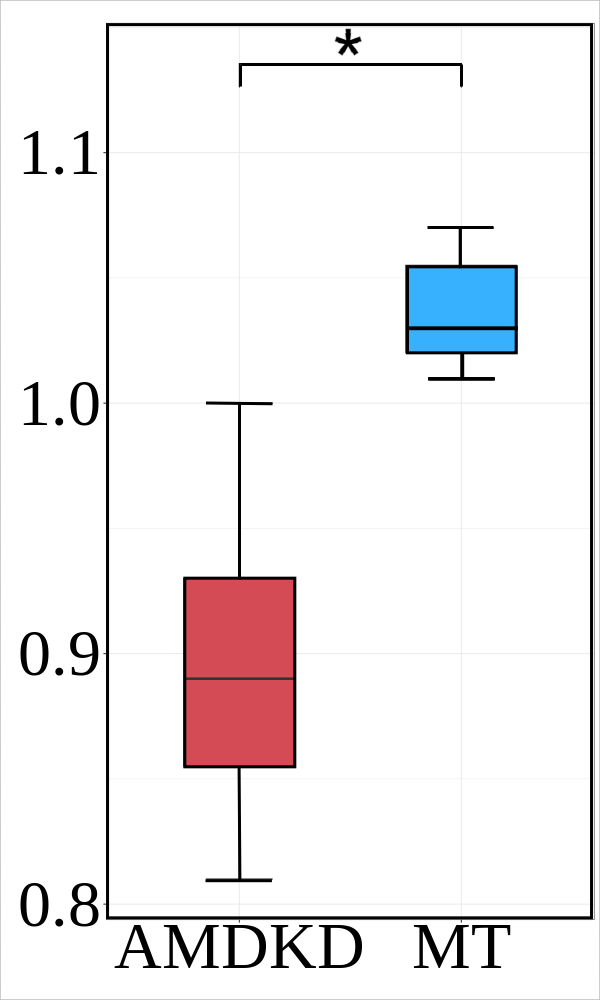
Figure 4: Boxplot of the overall gaps of AMDKD and its MT version. Here, $\star$ in the plot means that the two models are much different with statistical significance $p$-value = 0.02 < 0.05 (Wilcoxon test).

C.2 Effects of validation datasets.

Recall that the adaptive probability of teacher selection in Eq. (5) is calculated by the real-time performance of student model on the validation datasets, we further investigate whether the size of the validation datasets $\mathcal{V}$ will largely influence AMDKD. As displayed in Figure 5 and Figure 6, increasing the size of $\mathcal{V}$ (from 1,000 to 2,000) slightly improves the performance of AMDKD (but with no statistical significance), whereas decreasing the size of $\mathcal{V}$ (from 1,000 to 500) slightly impairs the performance of AMDKD (also with no statistical significance), which indicates that the good performance of AMDKD may not rely on the size of the validation datasets. Meanwhile, performing student model evaluation in each epoch inevitably introduces additional computation cost, where larger size of the validation datasets will cause longer training time. However, we note that the increment of validation in training time is acceptable when we use $\mathcal{V}$ = 1,000. Taking AMDKD-AM training on CVRP-100 as an example, the total evaluation time is 2.7s (0.9s per exemplar distribution on average) for each epoch, which is approximately 1% of the total training time (i.e., 4 min). What’s more, we note that the likelihood of selecting different teacher models would eventually converge to a stable one, which means that we may stop such evaluation early to speed up the training further if needed. For example, for training AMDKD-AM on CVRP-100 (see Figure 7), we may stop the student evaluation early at around 3,000 epochs.

Figure 5: Boxplot of the overall gaps of AMDKD-AM (with size of $\mathcal{V}$=1,000, red) and AMDKD-AM (with size of $\mathcal{V}$=2,000, blue) on CVRP-50. The "ns" in the plot means that the two models are not sigificantly different with statistical significance $p$-value = 0.25 $>$ 0.1 (Wilcoxon test).

Figure 6: Boxplot of the overall gaps of AMDKD-AM (with size of $\mathcal{V}$=1,000, red) and AMDKD-AM (with size of $\mathcal{V}$=500, blue) on TSP-50. The "ns" in the plot means that the two models are not sigificantly different with statistical significance $p$-value = 0.36 $>$ 0.1 (Wilcoxon test).

Figure 7: Likelihood of teacher selection along the epochs (AMDKD-AM on CVRP-100).

C.3 Effects of different hyper-parameters.

We further discuss the influence of the hyper-parameters on the performance of AMDKD.

• The starting epoch of the adaptive teacher selection strategy ($E^{\prime}$): it indicates the epoch to start our adaptive strategy for teacher selection. We include this hyper-parameter because preliminary experiments revealed that there could be a point in the learning curve (i.e., the reward convergence curve) where the training curves without and with (starting at the first epoch $E^{\prime}$=1) the adaptive strategy may meet. This suggests that there might be a sweet spot to implement the proposed adaptive strategy. For AMDKD-AM, the sweet spot is around $E^{\prime}$=500. And for AMDKD-POMO, we do not observe such a pattern and thus we use $E^{\prime}$)=1. In figure 8, we provide an example of how $E^{\prime}$ will affect the performance of AMDKD-AM.

• Number of steps per epoch ($T$): it indicates how long will the student model learn from the selected teacher before it possibly switches to a new one, which should not be too small or too large. As for POMO, the original $T$ is about 20, and we did not change it. As for AM, the original $T$ is about 2,500, and we empirically reduce it to 250 for a better trade-off.

• The total number of training epochs ($E$): it mainly follows the settings of the original backbone. In this paper, we employ different training epochs for different sizes and tasks since the hardness of the task itself may grow with size, which may require more steps to converge. Training curves of AMDKD-POMO (for CVRP) are depicted in Figure 9.

Figure 8: Boxplot of the overall gaps of AMDKD-AM ($E^{\prime}$=500, red) and AMDKD-AM ($E^{\prime}$=1, blue) on CVRP-50. The "ns" in the plot means that the two models are not significantly different with statistical significance $p$-value = 0.37 $>$ 0.1 (Wilcoxon test).

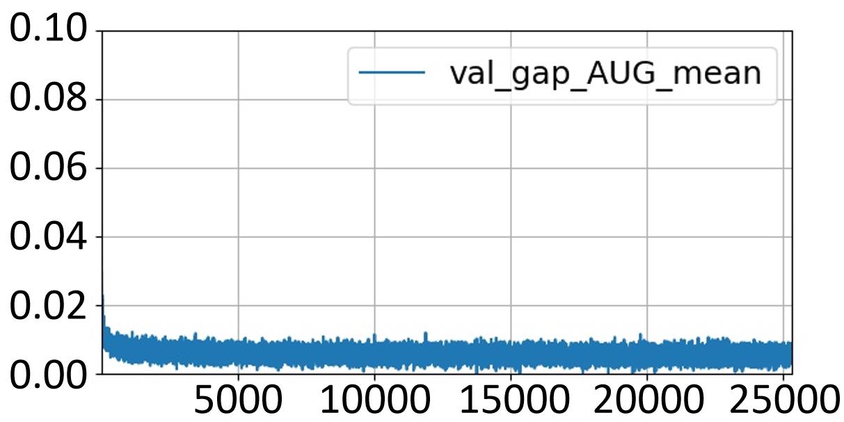
(a)

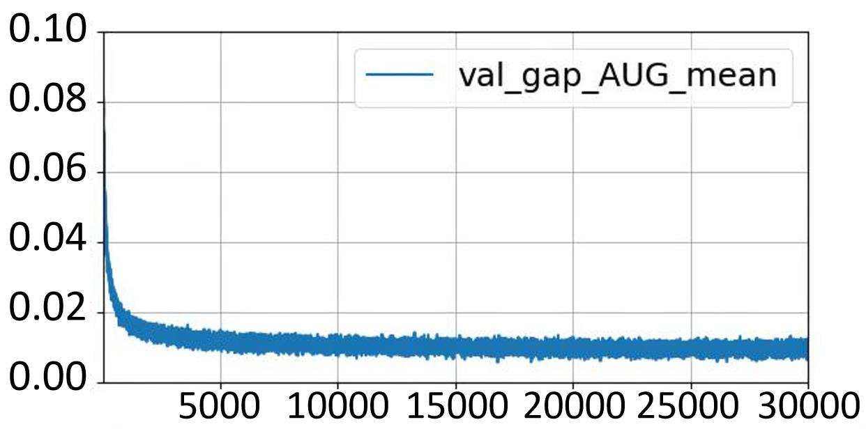
(b)

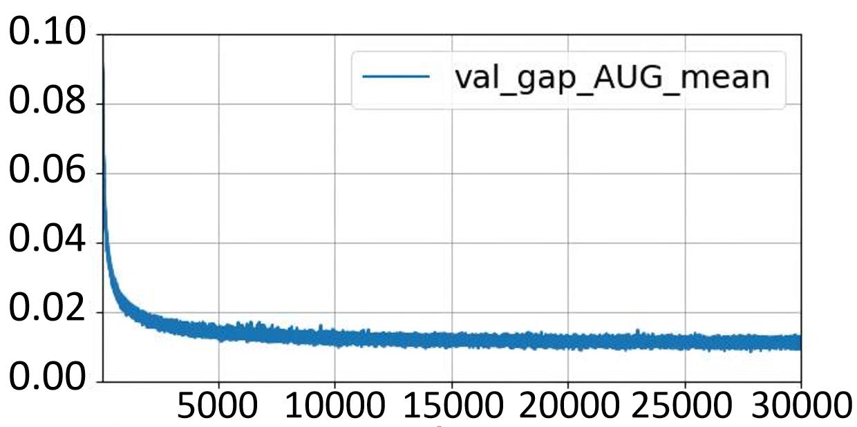
(c)

Figure 9: Training curves of AMDKD-POMO for solving CVRP. The x-axis is the epoch and the y-axis is the average gaps on the used three exemplar distributions.

C.4 Stability studies of AMDKD.

To demonstrate the stability of our experiment results, we take CVRP-50 as an example and independently run our trained AMDKD-AM and AM^# for 10 times, where we adopt different random seeds during the sampling process. As shown in Figure 10, both AMDKD-AM and AM^# exhibit extremely small fluctuations (even less than 0.001) when running with different seeds. Based on the Wilcoxon test, our AMDKD-AM significantly (with $p$-value < 0.001) outperforms AM^# on every unseen in-distributions and OoD distributions. As for AMDKD-POMO and POMO^#, the greedy decoding strategy is adopted, hence the results are expected to be stable with almost no fluctuation.

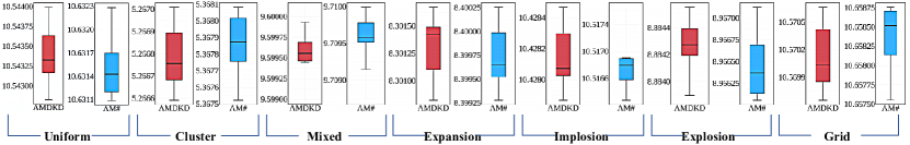
Figure 10: Experiment results of AMDKD-AM (red) and AM^# (blue) with different random seeds.

Appendix D Detailed results on benchmark datasets

We present the detailed results of benchmark dataset in Table 7 (TSPLIB) and Table 8 (CVRPLIB), respectively.

As displayed, models that have only been trained on the uniform distribution, i.e., AM and POMO, perform extremely poorly when inferring instances that may follow unknown distributions from the benchmark. The upgraded POMO^# significantly outperforms POMO, which seemingly alleviates this issue through training on our exemplar distributions, however, this simple strategy does not work well with AM. Regarding the prior cross-distribution generalization methods including GANCO, HAC, PSRO and DROP which show the potential to improve AM or POMO, their results are still far from satisfactory, where the performance of DROP are even inferior to POMO^# trained on our exemplar distributions. Nevertheless, our AMDKD not only outperforms all these baselines, but also brings a much more significant improvement over the backbone AM and POMO than those baselines do. Meanwhile, our AMDKD-POMO exhibits a much better generalization over POMO^# on CVRPLIB. Finally, we note that AMDKD equipped with EAS performs the best among all baselines, even achieving the optimal solution on some instances (e.g., KroA100, KroD100, lin105 in TSPLIB and X-n110-k14 in CVRPLIB). This leads to a new state-of-the-art performance for neural methods on these benchmark datasets. Finally, we list the full generalization results of our AMDKD in Table 9 (TSPLIB) and Table 10 (CVRPLIB), respectively.

Table 7: Detailed generalization results on selected instances from TSPLIB.

Instance	Opt.	PSRO	AM	GANCO	HAC	AM#	AMDKD-AM	POMO	DROP	POMO#	AMDKD-POMO	AMDKD+EAS
KroA100	21282	21703	46621	21908	21838	22138	21650	38452	24623	21285	21285	21282
KroB100	22141	22855	37921	22956	23110	23189	22350	33521	24874	22197	22233	22195
KroC100	20749	21079	34258	21139	21068	22326	21279	30736	24785	20751	20752	20947
KroD100	21294	21828	36141	21929	22625	23093	21863	29512	23257	21352	21314	21294
KroE100	22068	22532	29628	23174	22807	22865	22327	26829	26057	22179	22185	22111
lin105	14379	15372	15148	15478	15003	16865	14988	14922	14688	14430	14430	14379
pr107	44303	45288	53846	45393	47250	76152	46146	52846	47853	44647	45022	44347
Avg. Gap	0.00%	2.93%	55.19%	3.80%	4.16%	16.80%	2.50%	37.63%	12.14%	0.31%	0.44%	0.21%
($n$=100-150)
ch150	6528	6866	6930	6704	6852	6680	6669	6844	6709	6574	6609	6554
rat195	2323	2600	2612	2585	2638	3237	2550	2554	2403	2422	2432	2406
kroA200	29368	31450	35637	31741	33174	34294	31112	34972	34275	29840	29906	29931
Avg. Gap	0.00%	8.06%	13.32%	7.36%	10.50%	19.48%	5.96%	11.29%	7.64%	2.19%	2.59%	1.96%
($n$=150-200)

Table 8: Detailed generalization results on selected instances from CVRPLIB.

Instance	Opt.	AM	AM#	AMDKD-AM	POMO	DROP	POMO#	AMDKD-POMO	AMDKD+EAS
X-n101-k25	27591	38264	30327	30782	29484	28949	30510	29299	27855
X-n106-k14	26362	27923	27958	27279	27762	27308	27077	26847	26550
X-n110-k13	14971	16320	15668	15348	15896	15386	15175	15315	14971
X-n115-k10	12747	14055	14638	13366	13952	13783	13609	13418	12883
X-n120-k6	13332	14456	16094	14162	14351	14058	13997	13604	13457
X-n125-k30	55539	74329	68870	58507	69560	61382	62383	58570	56596
X-n129-k18	28940	30869	30833	29851	30155	30075	29597	29449	29007
X-n134-k13	10916	13952	12709	12573	13483	12846	11325	11330	11073
X-n139-k10	13590	14893	14953	14097	14132	13979	14053	13955	13704
X-n143-k7	15700	18251	18345	16509	17923	17682	16487	16346	15871
Avg. Gap	0.00%	16.65%	13.00%	6.12%	10.66%	7.25%	5.32%	3.54%	0.92%
($n=$100-150)
X-n153-k22	21220	38423	24722	23766	26386	24386	23629	23590	21849
X-n157-k13	16876	22051	19890	17539	19978	18378	17950	17450	17093
X-n181-k23	25569	27826	27314	26415	27428	27094	29014	26756	25736
X-n190-k8	16980	37820	21020	21162	22310	19864	18912	17575	17228
X-n200-k36	58578	76528	66298	62335	73135	64921	62228	62967	60562
Avg. Gap	0.00%	54.79%	15.63%	10.06%	21.25%	11.52%	9.76%	6.04%	1.95%
($n=$150-200)

Table 9: Full generalization results on TSPLIB (instances ranged from 100 to 200).

Instance	Opt.	AM#		AMDKD-AM		POMO#		AMDKD-POMO		AMDKD+EAS
		Obj.	Gap	Obj.	Gap	Obj.	Gap	Obj.	Gap	Obj.	Gap
kroA100	21282	22138	4.02%	21650	1.73%	21285	0.02%	21285	0.02%	21282	0.00%
kroB100	22141	23189	4.73%	22350	0.94%	22197	0.25%	22233	0.41%	22195	0.24%
kroC100	20749	22326	7.60%	21279	2.55%	20751	0.01%	20752	0.02%	20947	0.95%
kroD100	21294	23093	8.45%	21863	2.67%	21352	0.27%	21314	0.09%	21294	0.00%
kroE100	22068	22865	3.61%	22327	1.17%	22179	0.50%	22185	0.53%	22111	0.19%
eil101	629	663	5.45%	647	2.82%	641	1.90%	645	2.55%	629	0.00%
lin105	14379	16865	17.29%	14988	4.24%	14430	0.36%	14430	0.36%	14379	0.00%
pr107	44303	76152	71.89%	46146	4.16%	44647	0.78%	45022	1.62%	44347	0.10%
pr124	59030	62075	5.16%	60042	1.71%	59031	0.00%	59281	0.43%	59030	0.00%
bier127	118282	275748	133.13%	123211	4.17%	119232	0.80%	119052	0.65%	118729	0.38%
ch130	6110	6231	1.98%	6171	1.00%	6146	0.60%	6152	0.69%	6115	0.08%
pr136	96772	100194	3.54%	99912	3.24%	98478	1.76%	98215	1.49%	97487	0.74%
pr144	58537	66628	13.82%	60807	3.88%	59034	0.85%	58956	0.72%	58794	0.44%
ch150	6528	6680	2.33%	6669	2.16%	6574	0.70%	6609	1.25%	6554	0.40%
kroA150	26524	29501	11.22%	27354	3.13%	26723	0.75%	26808	1.07%	26538	0.05%
kroB150	26130	28585	9.39%	26820	2.64%	26334	0.78%	26328	0.76%	26152	0.08%
pr152	73682	85703	16.31%	78120	6.02%	74673	1.35%	75270	2.16%	75250	2.13%
rat195	2323	3237	39.35%	2550	9.77%	2422	4.25%	2432	4.68%	2406	3.57%
kroA200	29368	34294	16.77%	31112	5.94%	29840	1.61%	29906	1.83%	29931	1.92%
kroB200	29437	34074	15.75%	31968	8.60%	29665	0.77%	30132	2.36%	29765	1.11%
Avg. Gap		19.59%		3.63%		0.92%		1.18%		0.62%

Table 10: Full generalization results on CVRPLIB (instances ranged from 100 to 200).

Instance	Opt.	AM#		AMDKD-AM		POMO#		AMDKD-POMO		AMDKD+EAS
		Obj.	Gap	Obj.	Gap	Obj.	Gap	Obj.	Gap	Obj.	Gap
X-n101-k25	27591	30327	9.92%	30782	11.57%	30510	10.58%	29299	6.19%	27855	0.96%
X-n106-k14	26362	27958	6.06%	27279	3.48%	27077	2.71%	26847	1.84%	26550	0.71%
X-n110-k13	14971	15668	4.66%	15348	2.52%	15175	1.36%	15315	2.30%	14971	0.00%
X-n115-k10	12747	14638	14.83%	13366	4.86%	13609	6.76%	13418	5.27%	12883	1.07%
X-n120-k6	13332	16094	20.71%	14162	6.23%	13997	4.99%	13604	2.04%	13457	0.94%
X-n125-k30	55539	68870	24.00%	58507	5.34%	62383	12.32%	58570	5.46%	56596	1.90%
X-n129-k18	28940	30833	6.54%	29851	3.15%	29597	2.27%	29449	1.76%	29007	0.23%
X-n134-k13	10916	12709	16.43%	12573	15.18%	11325	3.74%	11330	3.79%	11073	1.44%
X-n139-k10	13590	14953	10.03%	14097	3.73%	14053	3.41%	13955	2.69%	13704	0.84%
X-n143-k7	15700	18345	16.84%	16509	5.15%	16487	5.01%	16346	4.12%	15871	1.09%
X-n148-k46	43448	61800	42.24%	52627	21.13%	53217	22.48%	46993	8.16%	44075	1.44%
X-n153-k22	21220	24722	16.50%	23766	12.00%	23629	11.35%	23590	11.17%	21849	2.96%
X-n157-k13	16876	19890	17.86%	17539	3.93%	17950	6.36%	17450	3.40%	17093	1.29%
X-n162-k11	14138	14762	4.41%	14663	3.72%	14951	5.75%	14903	5.41%	14543	2.86%
X-n167-k10	20557	21686	5.49%	21468	4.43%	21573	4.94%	21401	4.11%	20890	1.62%
X-n172-k51	45607	62419	36.86%	64444	41.30%	49844	9.29%	49741	9.06%	46340	1.61%
X-n176-k26	47812	53263	11.40%	51102	6.88%	54149	13.25%	53189	11.25%	49241	2.99%
X-n181-k23	25569	27314	6.83%	26415	3.31%	29014	13.47%	26756	4.64%	25736	0.65%
X-n186-k15	24145	25845	7.04%	25526	5.72%	25827	6.97%	26332	9.06%	24893	3.10%
X-n190-k8	16980	21020	23.79%	21162	24.63%	18912	11.38%	17575	3.50%	17228	1.46%
X-n195-k51	44225	57830	30.76%	60882	37.66%	48907	10.59%	51284	15.96%	45758	3.47%
Avg. Gap		15.87%		10.76%		8.05%		5.77%		1.55%

Appendix E Used assets and licenses

Table 11 lists the used assets in our work, which are all open-source for academic research. For our code and used data (new assets), we are using the MIT License.

Table 11: Used assets and their licenses.

Type	Asset	License	Usage
Code	Gurobi [5]	Free Academic lisence	Evaluation
	LKH3 [4]	Available for academic use	Evaluation
	AM [10]	MIT License	Remodification and evaluation
	POMO [12]	MIT License	Remodification and evaluation
	LCP [13]	MIT License	Remodification and evaluation
	HAC [17]	MIT License	Remodification and evaluation
	EAS [23]	MIT License	Remodification and evaluation
	DACT [14]	MIT License	Remodification and evaluation
	tspgen [43]	GNU General Public License v3.0	Generating datasets
Datasets	TSPLIB [42]	Available for any non-commerial use	Testing
	CVRPLIB [22]	Available for any non-commerial use	Testing

References

- Duan et al. [2020] Lu Duan, Yang Zhan, Haoyuan Hu, Yu Gong, Jiangwen Wei, Xiaodong Zhang, and Yinghui Xu. Efficiently solving the practical vehicle routing problem: A novel joint learning approach. In Proceedings of the 26th ACM SIGKDD International Conference on Knowledge Discovery & Data Mining, pages 3054–3063, 2020.
- Konstantakopoulos et al. [2020] Grigorios D Konstantakopoulos, Sotiris P Gayialis, and Evripidis P Kechagias. Vehicle routing problem and related algorithms for logistics distribution: A literature review and classification. Operational Research, pages 1–30, 2020.
- Qin et al. [2020] Zhiwei Qin, Xiaocheng Tang, Yan Jiao, Fan Zhang, Zhe Xu, Hongtu Zhu, and Jieping Ye. Ride-hailing order dispatching at DiDi via reinforcement learning. INFORMS Journal on Applied Analytics, 50(5):272–286, 2020.
- Helsgaun [2017] Keld Helsgaun. LKH-3 (version 3.0.7), 2017. URL http://webhotel4.ruc.dk/~keld/research/LKH-3/.
- Gurobi Optimization, LLC [2022] Gurobi Optimization, LLC. Gurobi Optimizer Reference Manual, 2022. URL https://www.gurobi.com.
- Croes [1958] G. A. Croes. A method for solving traveling-salesman problems. Operations Research, 6:791–812, 1958.
- Shaw [1997] Paul Shaw. A new local search algorithm providing high quality solutions to vehicle routing problems, 1997.
- Vinyals et al. [2015] Oriol Vinyals, Meire Fortunato, and Navdeep Jaitly. Pointer networks. In Advances in Neural Information Processing Systems, volume 28, pages 2692–2700, 2015.
- Nazari et al. [2018] Mohammadreza Nazari, Afshin Oroojlooy, Martin Takáč, and Lawrence V Snyder. Reinforcement learning for solving the vehicle routing problem. In Advances in Neural Information Processing Systems, pages 9861–9871, 2018.
- Kool et al. [2018] Wouter Kool, Herke van Hoof, and Max Welling. Attention, learn to solve routing problems! In International Conference on Learning Representations, 2018.
- Joshi et al. [2019] Chaitanya K Joshi, Thomas Laurent, and Xavier Bresson. An efficient graph convolutional network technique for the travelling salesman problem. arxiv preprint arxiv:1906.01227, ArXiV, 2019.
- Kwon et al. [2020] Yeong-Dae Kwon, Jinho Choo, Byoungjip Kim, Iljoo Yoon, Youngjune Gwon, and Seungjai Min. POMO: Policy optimization with multiple optima for reinforcement learning. In Advances in Neural Information Processing Systems, volume 33, pages 21188–21198, 2020.
- Kim et al. [2021] Minsu Kim, Jinkyoo Park, and joungho kim. Learning collaborative policies to solve np-hard routing problems. In Advances in Neural Information Processing Systems, volume 34, pages 10418–10430, 2021.
- Ma et al. [2021] Yining Ma, Jingwen Li, Zhiguang Cao, Wen Song, Le Zhang, Zhenghua Chen, and Jing Tang. Learning to iteratively solve routing problems with dual-aspect collaborative transformer. In Advances in Neural Information Processing Systems, volume 34, pages 11096–11107, 2021.
- Xin et al. [2021a] Liang Xin, Wen Song, Zhiguang Cao, and Jie Zhang. NeuroLKH: Combining deep learning model with Lin-Kernighan-Helsgaun heuristic for solving the traveling salesman problem. In Advances in Neural Information Processing Systems, volume 34, pages 7472–7483, 2021a.
- Zhang et al. [2022a] Rongkai Zhang, Cong Zhang, Zhiguang Cao, Wen Song, Puay Siew Tan, Jie Zhang, Bihan Wen, and Justin Dauwels. Learning to solve multiple-TSP with time window and rejections via deep reinforcement learning. IEEE Transactions on Intelligent Transportation Systems, pages 1–12, 2022a. doi: 10.1109/TITS.2022.3207011.
- Zhang et al. [2022b] Zeyang Zhang, Ziwei Zhang, Xin Wang, and Wenwu Zhu. Learning to solve travelling salesman problem with hardness-adaptive curriculum. In AAAI Conference on Artificial Intelligence, 2022b.
- Xin et al. [2022] Liang Xin, Wen Song, Zhiguang Cao, and Jie Zhang. Generative adversarial training for neural combinatorial optimization models, 2022. URL https://openreview.net/forum?id=9vsRT9mc7U.
- Geisler et al. [2022] Simon Geisler, Johanna Sommer, Jan Schuchardt, Aleksandar Bojchevski, and Stephan Günnemann. Generalization of neural combinatorial solvers through the lens of adversarial robustness. In International Conference on Learning Representations, 2022.
- Wang et al. [2022] Chenguang Wang, Yaodong Yang, Congying Han, Tiande Guo, Haifeng Zhang, and Jun Wang. A game-theoretic approach for improving generalization ability of TSP solvers, 2022. URL https://openreview.net/forum?id=7AssAnH5vyJ.
- Jiang et al. [2022] Yuan Jiang, Yaoxin Wu, Zhiguang Cao, and Jie Zhang. Learning to solve routing problems via distributionally robust optimization. In AAAI Conference on Artificial Intelligence, 2022.
- Uchoa et al. [2017] Eduardo Uchoa, Diego Pecin, Artur Pessoa, Marcus Poggi, Thibaut Vidal, and Anand Subramanian. New benchmark instances for the capacitated vehicle routing problem. European Journal of Operational Research, 257(3):845–858, 2017.
- Hottung et al. [2022] André Hottung, Yeong-Dae Kwon, and Kevin Tierney. Efficient active search for combinatorial optimization problems. In International Conference on Learning Representations, 2022.
- Bello et al. [2017] Irwan Bello, Hieu Pham, Quoc V Le, Mohammad Norouzi, and Samy Bengio. Neural combinatorial optimization with reinforcement learning. In International Conference on Machine Learning (Workshop), 2017.
- Vaswani et al. [2017] Ashish Vaswani, Noam Shazeer, Niki Parmar, Jakob Uszkoreit, Llion Jones, Aidan N Gomez, Łukasz Kaiser, and Illia Polosukhin. Attention is all you need. In Advances in Neural Information Processing Systems, volume 30, pages 6000–6010, 2017.
- Peng et al. [2019] Bo Peng, Jiahai Wang, and Zizhen Zhang. A deep reinforcement learning algorithm using dynamic attention model for vehicle routing problems. In International Symposium on Intelligence Computation and Applications, pages 636–650, 2019.
- Xin et al. [2021b] Liang Xin, Wen Song, Zhiguang Cao, and Jie Zhang. Multi-decoder attention model with embedding glimpse for solving vehicle routing problems. In AAAI Conference on Artificial Intelligence, pages 12042–12049, 2021b.
- Li et al. [2021] Jingwen Li, Yining Ma, Ruize Gao, Zhiguang Cao, Andrew Lim, Wen Song, and Jie Zhang. Deep reinforcement learning for solving the heterogeneous capacitated vehicle routing problem. IEEE Transactions on Cybernetics, 2021.
- Kwon et al. [2021] Yeong-Dae Kwon, Jinho Choo, Iljoo Yoon, Minah Park, Duwon Park, and Youngjune Gwon. Matrix encoding networks for neural combinatorial optimization. In Advances in Neural Information Processing Systems, volume 34, 2021.
- Zhang et al. [2022c] Zizhen Zhang, Zhiyuan Wu, Hang Zhang, and Jiahai Wang. Meta-learning-based deep reinforcement learning for multiobjective optimization problems. IEEE Transactions on Neural Networks and Learning Systems, 2022c.
- Dai et al. [2017] Hanjun Dai, Elias B Khalil, Yuyu Zhang, Bistra Dilkina, and Le Song. Learning combinatorial optimization algorithms over graphs. In Advances in Neural Information Processing Systems, pages 6351–6361, 2017.
- Fu et al. [2021] Zhang-Hua Fu, Kai-Bin Qiu, and Hongyuan Zha. Generalize a small pre-trained model to arbitrarily large TSP instances. In AAAI Conference on Artificial Intelligence, 2021.
- Kool et al. [2021] Wouter Kool, Herke van Hoof, Joaquim Gromicho, and Max Welling. Deep policy dynamic programming for vehicle routing problems. arxiv preprint arxiv:2102.11756, ArXiV, 2021.
- Chen and Tian [2019] Xinyun Chen and Yuandong Tian. Learning to perform local rewriting for combinatorial optimization. In Advances in Neural Information Processing Systems, volume 32, pages 6281–6292, 2019.
- Hottung and Tierney [2020] André Hottung and Kevin Tierney. Neural large neighborhood search for the capacitated vehicle routing problem. In European Conference on Artificial Intelligence, 2020.
- Hottung and Tierney [2022] André Hottung and Kevin Tierney. Neural large neighborhood search for routing problems. Artificial Intelligence, page 103786, 2022.
- Wu et al. [2021a] Yaoxin Wu, Wen Song, Zhiguang Cao, Jie Zhang, and Andrew Lim. Learning improvement heuristics for solving routing problems. IEEE Transactions on Neural Networks and Learning Systems, 33(9):5057–5069, 2021a.
- Costa et al. [2020] Paulo da Costa, Jason Rhuggenaath, Yingqian Zhang, and Alp Eren Akçay. Learning 2-opt heuristics for the traveling salesman problem via deep reinforcement learning. In Asian Conference on Machine Learning, pages 465–480, 2020.
- Ma et al. [2022] Yining Ma, Jingwen Li, Zhiguang Cao, Wen Song, Hongliang Guo, Yuejiao Gong, and Yeow Meng Chee. Efficient neural neighborhood search for pickup and delivery problems. In Proceedings of the Thirty-First International Joint Conference on Artificial Intelligence, pages 4776–4784, 7 2022.
- Chen et al. [2022] Jinbiao Chen, Huanhuan Huang, Zizhen Zhang, and Jiahai Wang. Deep reinforcement learning with two-stage training strategy for practical electric vehicle routing problem with time windows. In International Conference on Parallel Problem Solving from Nature, pages 356–370. Springer, 2022.
- Zhang et al. [2021] Zizhen Zhang, Hong Liu, MengChu Zhou, and Jiahai Wang. Solving dynamic traveling salesman problems with deep reinforcement learning. IEEE Transactions on Neural Networks and Learning Systems, 2021.
- Reinelt [1991] Gerhard Reinelt. TSPLIB-A traveling salesman problem library. ORSA journal on computing, 3(4):376–384, 1991.
- Bossek et al. [2019] Jakob Bossek, Pascal Kerschke, Aneta Neumann, Markus Wagner, Frank Neumann, and Heike Trautmann. Evolving diverse tsp instances by means of novel and creative mutation operators. In Proceedings of the 15th ACM/SIGEVO Conference on Foundations of Genetic Algorithms, pages 58–71, 2019.
- Hinton et al. [2015] Geoffrey Hinton, Oriol Vinyals, and Jeff Dean. Distilling the knowledge in a neural network. arxiv preprint arxiv:1503.02531, ArXiV, 2015.
- Jiao et al. [2020] Xiaoqi Jiao, Yichun Yin, Lifeng Shang, Xin Jiang, Xiao Chen, Linlin Li, Fang Wang, and Qun Liu. TinyBERT: Distilling BERT for natural language understanding. In Findings of the Association for Computational Linguistics: EMNLP 2020, pages 4163–4174, 2020.
- Liu et al. [2020] Weijie Liu, Peng Zhou, Zhiruo Wang, Zhe Zhao, Haotang Deng, and Qi Ju. FastBERT: a self-distilling BERT with adaptive inference time. In Proceedings of the 58th Annual Meeting of the Association for Computational Linguistics, pages 6035–6044, 2020.
- Stanton et al. [2021] Samuel Stanton, Pavel Izmailov, Polina Kirichenko, Alexander A Alemi, and Andrew G Wilson. Does knowledge distillation really work? In Advances in Neural Information Processing Systems, volume 34, pages 6906–6919, 2021.
- Mobahi et al. [2020] Hossein Mobahi, Mehrdad Farajtabar, and Peter Bartlett. Self-distillation amplifies regularization in hilbert space. In Advances in Neural Information Processing Systems, volume 33, pages 3351–3361, 2020.
- Hu et al. [2018] Minghao Hu, Yuxing Peng, Furu Wei, Zhen Huang, Dongsheng Li, Nan Yang, and Ming Zhou. Attention-guided answer distillation for machine reading comprehension. In EMNLP, 2018.
- Furlanello et al. [2018] Tommaso Furlanello, Zachary Lipton, Michael Tschannen, Laurent Itti, and Anima Anandkumar. Born again neural networks. In Proceedings of the 35th International Conference on Machine Learning, volume 80 of Proceedings of Machine Learning Research, pages 1607–1616, 10–15 Jul 2018.
- Berseth et al. [2018] Glen Berseth, Cheng Xie, Paul Cernek, and Michiel Van de Panne. Progressive reinforcement learning with distillation for multi-skilled motion control. In International Conference on Learning Representations, 2018.
- Rusu et al. [2016] Andrei A Rusu, Sergio Gomez Colmenarejo, Çaglar Gülçehre, Guillaume Desjardins, James Kirkpatrick, Razvan Pascanu, Volodymyr Mnih, Koray Kavukcuoglu, and Raia Hadsell. Policy distillation. In ICLR (Poster), 2016.
- Wu et al. [2021b] Chuhan Wu, Fangzhao Wu, and Yongfeng Huang. One teacher is enough? pre-trained language model distillation from multiple teachers. In Findings of the Association for Computational Linguistics: ACL-IJCNLP 2021, pages 4408–4413, 2021b.
- Williams [2004] Ronald J. Williams. Simple statistical gradient-following algorithms for connectionist reinforcement learning. Machine Learning, 8:229–256, 2004.
- Guo et al. [2020] Qiushan Guo, Xinjiang Wang, Yichao Wu, Zhipeng Yu, Ding Liang, Xiaolin Hu, and Ping Luo. Online knowledge distillation via collaborative learning. In Proceedings of the IEEE/CVF Conference on Computer Vision and Pattern Recognition, pages 11020–11029, 2020.
- Zhang et al. [2022d] Quanshi Zhang, Xu Cheng, Yilan Chen, and Zhefan Rao. Quantifying the knowledge in a DNN to explain knowledge distillation for classification. IEEE Transactions on Pattern Analysis and Machine Intelligence, 2022d.