A Multi-Scale Picture of Magnetic Field and Gravity from Large-Scale Filamentary Envelope to Core-Accreting Dust Lanes in the High-Mass Star-Forming Region W51

Abstract

We present 230 GHz continuum polarization observations with the Atacama Large Milimeter/Submillimeter Array (ALMA) at a resolution of 0$\farcs 1$ ($\sim 540$ au) in the high-mass star-forming regions W51 e2 and e8. These observations resolve a network of core-connecting dust lanes, marking a departure from earlier coarser more spherical continuum structures. At the same time, the cores do not appear to fragment further. Polarized dust emission is clearly detected. The inferred magnetic field orientations are prevailingly parallel to dust lanes. This key structural feature is analyzed together with the local gravitational vector field. The direction of local gravity is found to typically align with dust lanes. With these findings we derive a stability criterion that defines a maximum magnetic field strength that can be overcome by an observed magnetic field-gravity configuration. Equivalently, this defines a minimum field strength that can stabilize dust lanes against a radial collapse. We find that the detected dust lanes in W51 e2 and e8 are stable, hence possibly making them a fundamental component in the accretion onto central sources, providing support for massive star formation models without the need of large accretion disks. When comparing to coarser resolutions, covering the scales of envelope, global, and local collapse, we find recurring similarities in the magnetic field structures and their corresponding gravitational vector fields. These self-similar structures point at a multi-scale collapse-within-collapse scenario until finally the scale of core-accreting dust lanes is reached where gravity is entraining the magnetic field and aligning it with the dust lanes.

1 Introduction

The formation and evolution of molecular clouds, the sites of high-mass star formation, are a complex interaction between gravity, turbulence, and magnetic fields, covering orders of magnitudes in physical length and density (e.g. Hennebelle & Inutsuka, 2019; Li et al., 2014; Crutcher, 2012). Moreover, a variety of feedback mechanisms add to the intricacy of the formation processes. Among all these constituents, the magnetic (B-)field still poses the likely biggest challenge to the establishment of a firm picture of star formation across time and scale. This has been largely due to the difficulty of detecting signals that originate from the presence of B-fields (as they are typically only at the percent level of non-magnetic signals) and the limited techniques to measure a B-field strength to gauge its significance against other constituents. Recent advances in observational capabilities, offering substantially improved sensitivities, are now rapidly changing this situation. Of particular interest are observations of dust continuum polarization. This is because a growing suite of instruments covering complete ranges in wavelengths and resolutions is available, and because dust polarization observations typically lead to the most connected and complete coverage in detections, unlike e.g., Zeeman observations that remain challenging and are often limited to more localized and small areas in a source.

When utilizing dust polarization observations in the (sub-)millimeter regime, dust grains are thought to be aligned with their shorter axis parallel to the B-field. Rotating detected polarization orientations by $90^{\circ}$ then yields magnetic field orientations (Cudlip et al., 1982; Hildebrand et al., 1984; Hildebrand, 1988; Lazarian, 2000; Andersson et al., 2015). At the densities and scales probed with the here presented observations, radiative torques can provide an explanation for this B-field-dust alignment (Draine & Weingartner, 1996, 1997; Lazarian, 2000; Cho & Lazarian, 2005; Lazarian & Hoang, 2007; Hoang & Lazarian, 2016). A growing literature is mapping magnetic field structures based on this property and investigating both statistical findings and detailed higher-resolution features. The survey conducted by Zhang et al. (2014) with the SubMillimeter Array (SMA) towards a sample of 14 high-mass star-forming regions resolving scales around 0.1 pc (resolutions $\theta$ of $1\arcsec$ to several arcseconds) at 345 GHz provides statistical evidence for magnetic fields playing an important role during the collapse and fragmentation of massive molecular clumps. Further enlarging this sample to 18 massive dense cores, the recent work in Palau et al. (2021) finds a tentative positive correlation between the number of fragments and the mass-to-flux ratio, hinting that magnetic fields can possibly suppress fragmentation. Investigating the role of the B-field in the infrared dark cloud G14.225$-$0.506 using the Caltech Submillimeter Observatory (CSO) observations with SHARP with $\theta\sim 10\arcsec$ at 350$\mu$m, Añez-López et al. (2021) find that different B-field morphologies and strengths can explain the different observed fragmentation properties. Also observed with the CSO/SHARP, the different fragmentation types in G34.43$+$0.24 are explained by a different relative significance of gravity, turbulence, and magnetic field (Tang et al., 2019). Observed with POL-2 on the James Clerk Maxwell Telescope (JCMT) with $\theta\sim 14\arcsec$ at 850 $\mu$m, the NGC 6634 filamentary network is resolved down to about 0.1 pc, revealing detailed B-field structures and variations across the main filament and sub-filaments (Arzoumanian et al., 2021). Higher-resolution (sub-)arcsecond observations with ALMA (mostly around 850 $\mu$m and 1.2 mm) have started to reveal detailed morphological features in the magnetic field, such as an expanding UCHII region in G5.89$-$0.39 leaving a clear imprint in the B-field morphology (Fernández-López et al., 2021), sharpening the earlier coarser SMA observations (Tang et al., 2009a); a highly fragmented filament in W43-MM1 (Cortes et al., 2016); a resolved hour-glass magnetic field structure in G31.41$+$0.31 (Beltrán et al., 2019); and ring-like and arm-like structures likely resulting from toroidal wrapping of the magnetic field in OMC-3 (Takahashi et al., 2019).

W51 is a high-mass star-forming complex at parallax distances around 5.41 kpc for W51 e2 and e8 (Sato et al., 2010) and 5.10 kpc for W51 North (Xu et al., 2009), located in a region with little foreground and background contamination. The entire complex shows star-formation activities at various evolutionary stages (Ginsburg et al., 2017; Saral et al., 2017; Ginsburg et al., 2015). Collimated small-scale SiO outflows are detected in W51e2-E, e8, and North (Goddi et al., 2020), and they appear to connect to larger-scale outflows seen in ¹²CO(2–1) in all three sources (Ginsburg et al., 2017) and also in ¹²CO(3–2) in e2-E (Shi et al., 2010). The plane-of-sky B-field morphology has been mapped with a series of polarization observations with increasingly higher angular resolutions $\theta$, starting from the earliest interferometric observations with BIMA ($\theta\sim 3\arcsec$; Lai et al., 2001) to the SMA ($\theta\sim 0\farcs 7$; Tang et al., 2009b, 2013) and to the first observations with ALMA ($\theta\sim 0\farcs 26$; Koch et al., 2018). The BIMA observations at 1.3 mm showed W51 e2 and e8 as an elongated connected north-south structure with a magnetic field mostly perpendicular to it (Lai et al., 2001). The e2 region manifested itself as a clear polarization hole. The higher-resolution SMA observations at 0.87 mm revealed more complex magnetic field structures which are likely the reason for the depolarization in the larger BIMA beam. The finer B-field structures in e2 and e8 showing hourglass-like topologies with clearly bent field lines were interpreted as gravitational collapse imprinted onto the B-field morphology (Tang et al., 2009b). The first ALMA observations at 1.3 mm (Koch et al., 2018), again improving the resolution by a factor of 10 in area, revealed striking new features. In particular, they clearly resolved the satellite core e2-NW with bow-shock shaped B-field structures that are hinting infall of this smaller core towards the dominating mass center e2-E. Additionally, areas with centrally converging symmetrical B-field structures (convergence zones) and possibly streamlined B-field morphologies were detected. A generic feature seen in many of the resolved cores inside e2, e8, North, and also on larger scale between e2 and e8, is B-field structures resembling gravitational pull towards the core’s center on one side with the other side showing B-field lines appearing to be dragged away towards the next more massive neighboring core. This imprint in the B-field morphology was interpreted as a scenario where local collapse is ongoing while a locally collapsing core, as an entity, is pulled to the next more massive gravitational center which itself is also collapsing (Koch et al., 2018). Recent numerical work by Vázquez-Semadeni et al. (2019) is exactly presenting such a scenario as a result of a global hierarchical collapse where a flow regime leads to collapses within collapses.

While the successively higher-resolution observations in W51 keep revealing new magnetic field features from imprints of dynamical processes, the W51 region has, at the same time, served as a mine of information for our developments of new analysis techniques. The SMA observations (Tang et al., 2009b) served as a testbed for the polarization–intensity gradient technique (Koch et al., 2012a, b). This technique uses the measurable angle $\delta$ between a magnetic field orientation and an intensity gradient as a key observable which, in combination with a second angle between intensity gradient and local gravity, makes it possible to derive a magnetic field strength. The technique gives a local magnetic field strength – at every position where a magnetic field orientation is detected – and therefore, leads to maps of field strengths. At the same time, the technique puts forward a magnetic field-to-gravity force ratio, $\Sigma_{\rm{B}}$, based solely on measurable angles which allows for a completely independent estimate of a mass-to-flux ratio (Koch et al., 2012b). The establishment of $\delta$ as a prime observable as well as an approximation for $\Sigma_{\rm{B}}$ is presented in Koch et al. (2013) with an application to a 50-source sample of low- and high-mass star-forming sources in Koch et al. (2014). A main result from this series of papers is the recognition of a spatially varying role of the magnetic field, e.g., mass-to-flux ratios can transition from outer sub-critical to inner super-critical areas in a star-forming region, and force ratios $\Sigma_{\rm{B}}$ are clearly varying from zones where collapse and infall are slowed down or prohibited by the magnetic field to other zones, within the same source, where collapse is possible. With the first ALMA data in Koch et al. (2018) an additional measure was introduced, the $\sin\omega$ measure. The angle $\omega$, in the range between 0 and $90^{\circ}$, measures the projection of the local magnetic field tension force along the local direction of gravity, and hence quantifies the fraction (in a range of 0 to 1) of the magnetic field tension force that can work against the gravitational pull. Maps of $\sin\omega$ of all the cores in W51 e2, e8, and North systematically display zones where the magnetic field is maximally opposing gravity and other zones where the magnetic field is nearly or completely ineffective in slowing down gravity (Koch et al., 2018). It should be noted that all of these techniques are utilizing a combination of the geometry and shape of both the magnetic field and the underlying emission (density) structures to infer the local role of the magnetic field.

As presented in the following sections, this current work is resolving once more finer structures with a resolution of $\theta\sim 0\farcs 1$, an improvement in area by a factor of 7 over the earlier $0\farcs 26$ observations, reaching a physical length scale of about 2.6 mpc or 540 au at the distance of W51 e2/e8. With this, the earlier near-spherical structures are resolved, revealing connecting dust lanes. Together with earlier observations covering larger scales we propose a synergetic multi-scale scenario of the evolving role of the magnetic field in the W51 high-mass star-forming region starting from the large filamentary envelope scale ($\sim 0.5$ pc), global-collapsing-core scale ($\sim 0.05$ pc), inside-core fragmenting scale ($\sim 10$ mpc) down to the scale of dust lanes ($\sim 2.6$ mpc) accreting onto central cores. The paper is organized as follows. Section 2 describes our ALMA observations. Polarization properties are given in the appendix. The detected key structural features are introduced in Section 3. Section 4 analyzes the gravitational vector field together with the magnetic field morphology and derives a stability criterion for filaments and fibers. The discussion in Section 5 presents a road towards a synergetic multi-scale picture.

2 Observations

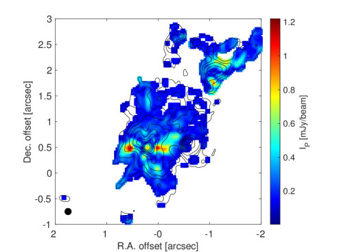
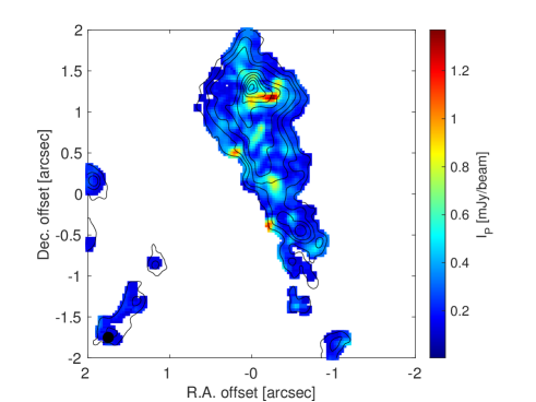
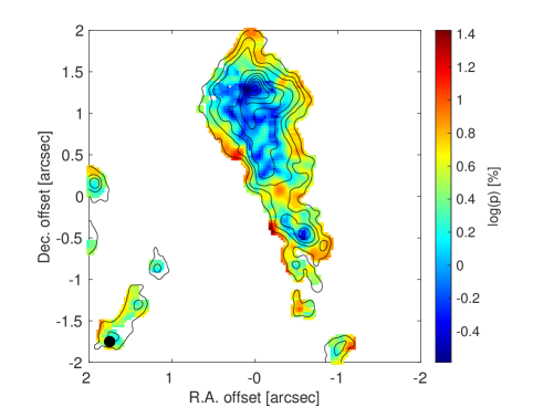
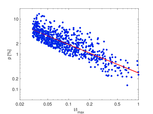
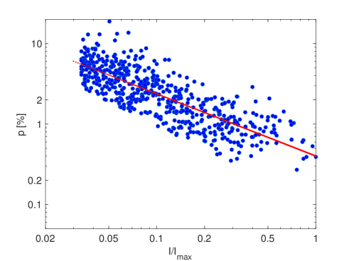
Figure 12: Top to bottom panels: polarized emission $I_{p}$, polarization percentage $p$, and polarization percentage versus Stokes $I$, normalized by $I_{\rm{max}}$, for W51 e2 (left column) and W51 e8 (right column). The red solid lines in the bottom panels are the best-fit power laws with indices $-0.81$ (e2) and $-0.77$ (e8). The maps display overgridded data for a sharper visualization. The data in the bottom panels are extracted from maps gridded to only half of the synthesized beam resolution.

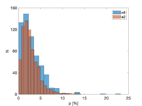
Figure 13: Histograms of polarization percentages for W51 e2 and e8. Averages, median values, and standard deviations are 2.8%, 2.3%, and 2.0% for e2, and 3.1%, 2.4%, and 2.5% for e8. Maximum and minimum polarizations are 14% and 0.13% for e2 and 23% and 0.27% for e8.

The project was observed with the ALMA Band 6 receiver (around a wavelength of 1.3 mm) in Cycle 4 and Cycle 5, project codes #2016.1.01484.S and #2017.1.01242.S. Observations were done in two execution blocks (EBs) on August 17, 2017. The two EBs were calibrated separately in flux, bandpass, and gain. The polarization calibrations were performed after merging the two calibrated EBs. The array included 44 antennas with (projected) baselines ranging from 21 m to 3638 m. The four basebands were set in TDM mode (64 channels for a 2 GHz bandwidth per baseband). The calibration (bandpass, phase, amplitude, flux) was performed using CASA v4.7.2. J1922+1530 (flux $\sim$ 0.219 Jy at 232.9 GHz) was used as a phase calibrator, and J1751+0939 and J1922+1530 were the flux calibrators. The phase centers for W51 e2 and e8 where (RA, DEC)$=$(19:23:43.95, $+$14:30:34.00) and (RA, DEC)$=$(19:23:43.90, $+$14:30:27.00), respectively, in J2000 coordinates. The presented images are with a Briggs weighting scheme and a robust parameter of 0.5, which gives an angular resolution of 0$\farcs$11$\times$0$\farcs$10, with a position angle PA of -23$\arcdeg$. The sensitivities of the Stokes I, Q, U images are 1.2 mJy/beam, 0.04 mJy/beam, and 0.04 mJy/beam, respectively. Polarization measurements $I_{p}=\sqrt{Q^{2}+U^{2}}>0$ are positively biased (while both $Q$ and $U$ can be negative). Hence, $I_{p}$ in the high signal-to-noise regime ($I_{p}\geq 3\sigma_{p}$) is debiased as $I_{p}=\sqrt{Q^{2}+U^{2}-\sigma_{Q,U}^{2}}$, where $\sigma_{Q}\approx\sigma_{U}$ are the noise levels in $Q$ and $U$ (Leahy, 1989; Wardle & Kronberg, 1974). Investigating instrumental polarization in Band 6, Nagai et al. (2016) conclude that linear polarization at a level of $<0.1$% is detectable. For images presented in this paper, the two simultaneous conditions of having Stokes $I\geq$3$\sigma$ and $I_{p}\geq$3$\sigma_{p}$ are imposed. Polarization averages are around 3%, with a single minimum value of about 0.1% and some isolated maximum values above 10%. Detailed polarization results are in the appendix and in Figures 12 and 13.

3 Observed Key Structural Features

In the following we are describing three new structural features in dust continuum Stokes $I$ and in dust polarization (B-field), seen in the $0\farcs 1$ ($\sim 2.6$  mpc or $\sim 540$ au) resolution ALMA observations of W51 e2 and e8: (1) resolved networks of dust lanes in Stokes $I$; (2) magnetic field morphology in dust lanes; (3) sectors of straight field lines around e2-E followed by an abrupt change in magnetic field orientations in the central core region.

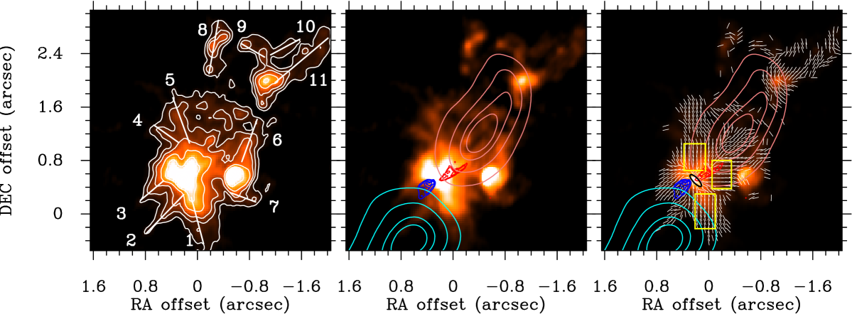
Figure 1: Dust continuum emission in color scale with a resolution of 0$\farcs$1 ($\sim$2.6 mpc or $\sim$ 540 au) around 230 GHz ($\sim 1.3$ mm) in Band 6 with ALMA for W51 e2, except the upper left panel which shows the earlier still more roundish detection with a 0$\farcs$26 resolution (Koch et al., 2018). White segments display the magnetic field in the right panels at half of the synthesized beam resolution (white ellipses in the lower left corners). Outflows are over-plotted in the bottom middle and right panel. The cyan and faint-red contours denote the blue- and red-shifted ¹²CO 2-1 outflow component, and the blue and red contours mark the blue- and red-shifted SiO 5-4 outflow emission. Dust lanes and streamers are labelled in the bottom left panel where continuum contours are identical to the ones described in the right panels in Figure 8. The bottom right panel marks the sectors of nearly straight field lines (yellow rectangles) and the possible small disk (black ellipse) as discussed in section 3.

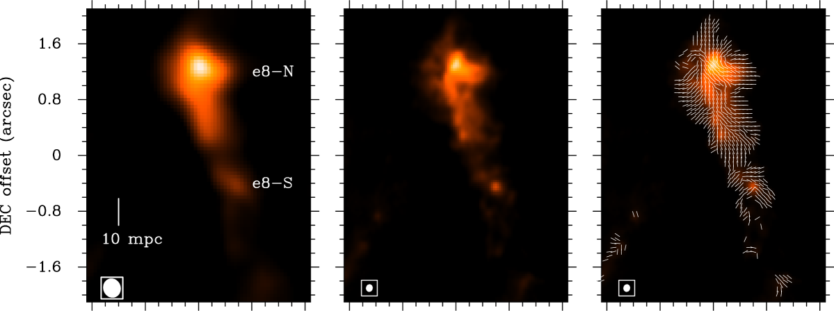
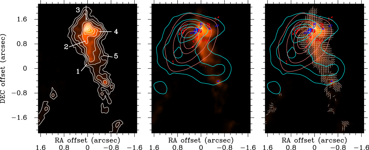
Figure 2: Identical to Figure 1 but for W51 e8.

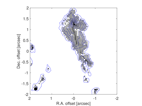
Figure 3: Local gravitational vector fields $\mathbf{g}_{\rm{loc}}$ for W51 e2 (left panel) and e8 (right panel) overlaid on dust continuum contours (blue). Vectors are displayed with a uniform length, giving the direction but not the absolute magnitude of local gravity. Vectors are selectively shown for the locations where polarized emission is detected and displayed at half of the synthesized beam resolution.

Departure from spherical continuum structures – resolved networks of core-connecting dust lanes. Earlier SMA ($\theta\sim 3\arcsec-0\farcs 7$; Tang et al., 2009b) and ALMA ($0\farcs 26$; Koch et al., 2018) observations showed dust continuum structures that appeared circular (e2) and smoothly elongated (e8), with no indications yet of resolved shapes, sizes, and their surroundings. Improving the resolution from the ALMA $0\farcs 26$ to our latest ALMA $0\farcs 1$ observations – giving a finer resolution of about a factor of 7 in area – starts to reveal a radically different picture (Figure 1 and 2). The cores e2-E, e2-W, e2-NW, e8-N, and e8-S do not seem to fragment further. The previously circular dust continuum emission around these cores is resolved into streamer-like lanes that appear to connect to the central and more compact cores. All these lanes appear to either come in from the cores’ peripheries or they form connections between individual cores. For e2, we start to resolve a network of dust lanes, converging towards e2-E and e2-W. The satellite core e2-NW is further resolved into three tail-like streamers (feature 9, 10, and 11, as labelled in the bottom left panel in Figure 1) where two are along a NW-SE direction. A more isolated lane in the north (lane 8), west of e2-NW, is pointing to the main core e2-E. Around the dominating agglomerate e2-E/e2-W we find at least seven dust lanes (lane 1 to 7), all roughly radially pointing to the central agglomerate. They vary in their resolved widths from about $0\farcs 1$ to $0\farcs 4$ ($\sim 540$ au to $2,000$ au) with lengths around $0\farcs 5$ before merging into the central denser cores. W51 e8 (Figure 2, bottom left panel) displays a main north-south connection between e8-S and e8-N with a width and length of about $0\farcs 5$ and 1″, respectively. The e8-N core shows three main emerging lanes from its surrounding, namely from the south, north, and west (lanes 2, 3, and 4). Two possible lanes, hinted by outward bulking contours (lanes 1 and 5), are merging into the main north-south connection. Though being evident in their emerging shape, these extensions and dust lanes are not yet as clear as in W51 e2. Section 4.1 with Figure 3 and 4 motivates and explains these dust lanes based on the underlying gravitational structures.

Magnetic field in dust lanes. With the resolved dust continuum structures, the plane-of-sky projected magnetic field morphology is also resolved in the dust lanes. The B-field orientations are prevailingly aligned parallel along the dust lanes. In W51 e2, the B-field is observed to be parallel in the three dust lanes 1 to 3 in the south converging to e2-E (Figure 1, bottom left and top right panel), and also in the lane in the north (lane 5). Almost no polarization is detected along the northeastern dust lane (lane 4). The e2-E and e2-W cores appear connected with straight field lines. No or only very incomplete polarization is detected in the emerging lane 7 in the west of e2-W. The longer tail-like streamer of e2-NW (lane 11) shows a B-field morphology clearly aligned with the tail. The thinner northern tail (lane 10) has an initial field structure that appears perpendicular to the tail in its northern tip while then becoming more aligned moving along the tail to the south. The dust lane 8 is disconnected and displays varying field orientations. Since W51 e8 is not yet as resolved as e2, our observations seem to additionally capture the transition in the B-field structures from the surrounding diffuse material to the (relatively denser) emerging dust lanes (Figure 2, bottom left and top right panel). The region between e8-S and e8-N illustrates this. The thin bridge immediately north of e8-S (around offset (R.A., Dec.)$\sim(-0.25,-0.1)$) already shows a B-field along a north-south axis. Moving further north, the B-field on the lower contour levels on the east and west side is mostly perpendicular to while progressively bending and getting aligned with the e8-N – e8-S axis in the inner relatively denser spine region of the main north-south connection. This feature is very similar to the findings in W51 e2 with the coarser resolution of $0\farcs 26$ (Koch et al., 2018) where field lines symmetrically converging from two sides towards a central line were observed. This feature was named a convergence zone, and it was interpreted as material being accreted symmetrically from two sides towards a central region or channel. Since e8 appears less resolved, we might be seeing this same feature as already seen in e2 with coarser resolution. Hence, this transition from outer perpendicular lines to the inner more aligned field lines might be a more common feature. The dust lanes around e8-N (lanes 2, 3, and 4) have their field lines aligned and pointing towards the center of e8-N. The possible lanes 1 and 5 show field line orientations that follow the general trend of the convergence zone.

Straight magnetic field lines in three sectors around W51 e2-E and abrupt change in field orientations in the innermost center region. The magnetic field morphology shows nearly straight plane-of-sky projected field lines in three sectors around the Stokes $I$ emission peak of W51 e2-E (Figure 1, bottom right panel). All three sectors extend over an area of about $0\farcs 5\times 0\farcs 5$. The field lines within these sectors appear to be at 90$\arcdeg$ angles with respect to each other (from North, to West, to South), with field orientations along a north-south direction (northern and southern sector), and along an east-west direction (western sector). An overall trend of converging bent field lines towards e2-E is already seen in the coarser $0\farcs 26$ resolution image in Koch et al. (2018). The higher resolution maps here show strikingly straight field lines in three sectors around e2-E. Following the three sectors closer to the emission peak of e2-E, offset (R.A., Dec.)$\sim(0.2,0.5)$, the nearly straight B-field lines are abruptly changing orientations, forming a prevailingly northeast-southwest aligned structure. This structure is aligned roughly 45$\arcdeg$ with respect to the north-south and east-west field orientations in the three sectors. The change in orientation from the nearly straight outer field lines to this inner structure happens within one or two synthesized beams, with changes between adjacent field segments as large as almost 90$\arcdeg$. While the field morphologies in the three sectors and the centermost region are all coherent and connected, they are also clearly different. This likely indicates that these two regions are governed by two different physical processes. We note that both the blue- and red-shifted SiO outflow lobe seem to originate from where the magnetic field lines transition into the 45$\arcdeg$-oriented central field pattern (Figure 1, bottom right panel). As this outflow is interpreted as a signpost of an underlying not-yet-resolved disk (Goddi et al., 2020), we speculate that this innermost structure is capturing the B-field morphology towards and in this putative accretion disk. In W51 e8, the e8-N core shows close-to-straight incoming field lines towards its peak from the west, north and from the south (Figure 2, top right panel). Although not as regular as in e2-E, rapid changes in field orientations around 90$\arcdeg$ are also observed towards the peak location, where again an accretion disk is expected based on a detected SiO outflow (Figure 2, bottom right panel; Goddi et al., 2020).

4 Analysis

4.1 Direction of Local Gravity around Cores and in Dust Lanes

How is gravity acting in the connecting dust lanes in W51 e2 and e8? Calculating the local direction of gravity in the plane of sky was introduced in Koch et al. (2012a, b). In the following we are interested in identifying systematic patterns in the gravitational vector field, both in conjunction with the underlying Stokes $I$ dust continuum structures and the observed B-field morphology. Figure 3 presents maps of the directions of local gravity for e2 and e8.

A plane-of-sky projected direction and a relative magnitude of local gravity (at every location in a map) can be derived by summing up all the surrounding pixelized dust continuum emission. This sum is a vector sum that takes into account the directions and distances to every surrounding pixel weighted by the dust emission. This vector sum is calculated at every pixel (Koch et al., 2012a, b). In order to have a measure for how gravity is locally acting, we need to assume that the distribution of dust emission is a fair tracer for the distribution of the total mass in a source. If this is the case, we can visualize the direction of the local gravitational pull (Figure 3). The absolute magnitude of the gravitational pull is scalable by a gas-to-dust mass ratio. We note that an unknown (constant) gas-to-dust mass ratio does not change the directions of the local gravity vectors. This ratio is only needed in order to go from relative to absolute magnitudes. For the following analysis and discussion we assume that the observed dust distribution is closely enough tracing the overall mass distribution in W51 e2 and e8. In order to generate the gravitational vector fields in Figure 3, an upper and lower limit of distances needs to be defined within which the vector sum is calculated. The smallest scale is defined by the (synthesized) beam resolution, and the largest scale is given by the largest distance to any detected emission in our maps. As we have tested, diffuse emission at distances beyond the extension of our maps can be safely omitted. This is because this emission is down-weighted by a quickly dropping $1/r^{2}$ factor and, furthermore, the already diffuse emission tends to become more azimuthally symmetrical at larger distances which will lead to largely canceling out any gravitational pull.

W51 e2 reveals an overall radial vector field, with a main converging point towards e2-E. While vectors in the south, north, and west of e2-W are still pointing towards the emission peak of e2-W, the vectors in the eastern end of e2-W (around offset (R.A., Dec.)$\sim(-0.5,0.6)$) are already influenced by the locally dominating mass associated with e2-E. As a result, these vectors are already being deflected and turning towards e2-E. The satellite core e2-NW shows a pattern where local gravity vectors from the north, northwest, and northeast are converging around offset (R.A., Dec.)$\sim(-1.0,2.0)$. It is interesting to note that the extension from the peak of e2-NW towards south, until offset (R.A., Dec.)$\sim(-1.0,1.6)$, shows initial local gravity directions towards this converging point with a growing trend for directions turning away towards southwest (the dominating mass concentration around e2-E) the further one moves along this extension to the south. This trend of observing a local gravity field that is converging towards a local peak emission on one side while the other side shows gravity vectors being bent away to a neighboring more dominating mass concentration was already noted in the coarser resolution data of W51 e2, e8, and North in Koch et al. (2018). The present observations are further sharpening this picture, and they provide additional support for a local collapse scenario, where collapse can happen locally around this emission peaks while the underlying forming cores, as an entity, are being pulled to the neighboring larger mass concentration (see also discussion in section 5.2).

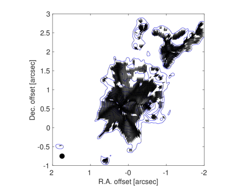
Figure 4: Identical to Figure 3 but with the gravitational vector field $\mathbf{g}_{\rm{loc}}$ oversampled to emphasize the gravitational local convergence towards ridges, before merging into local mass centers. These ridges form a gravitational skeleton (visible as thicker black zones) and are suggestive of gravitationally driven accretion regions and channels. This skeleton largely falls onto the dust lanes labelled in Figure 1 and 2.

The local gravity field in all the dust lanes around e2-E/W (lanes 1 to 7, bottom left panel in Figure 1) is overall radial. When overgridded for a better visualization, it additionally shows convergence towards ridges that form a gravitational skeleton (Figure 4) and likely are the underlying structures for the dust lanes seen in Figure 1 and 2. As such, local gravity is dominantly directed along dust lanes. The two lanes coming in from the NW connecting to e2-NW (lane 10 and 11) show a vector field mostly along their longer axes towards the e2-NW emission peak. The exceptions of this overall alignment between dust lanes and local gravity directions are the southern extension of e2-NW, around offset (R.A., Dec.)$\sim(-1.0,1.7)$, and dust lane 9. As discussed above for the southern extension, they both reveal a gravitational vector field being directed to the dominating southern e2-E/e2-W agglomerate.

We remark that both converging gravitational centers, around e2-E and e2-NW, show an offset with respect to their dust emission peaks. This offset is about $0\farcs 15$ for e2-E along a northwest direction (towards e2-NW), and it is about $0\farcs 25$ for e2-NW along a southeast direction (towards e2-E). While this might be due to e.g., projection effects or other forces that shape the dust distribution, the noted offsets are also close to our resolution. The precise reason for these possible offsets is being further investigated.

W51 e8 shows an overall radial vector field with a main converging point on e8-N around (R.A., Dec.)$\sim(0.0,1.2)$. Along its southern extension, this source displays a gravitational field that is converging to a north-south oriented ridge along R.A. $\sim 0.0$. From east and west the vector field is first streaming into this central ridge in the south before turning to become gradually more radial when approaching the e8-N core further north. The overall direction is pointing to the dominating e8-N core as far south as (R.A., Dec.)$\sim(-0.2,-0.1)$. The e8-S core is a local gravitational center around (R.A., Dec.)$\sim(-0.5,-0.5)$ with a clear converging field from the southwest. Moving further north along a southwest-northeast axis this vector field is gradually turning around, redirected, and aligning with the central ridge.

In summary, both e2 and e8 appear to have a single main gravitational center (e2-E and e8-N) with an overall simple radial-like gravitational vector field. When overgridding the gravitational field, finer structures become more visible pointing at radial ridges forming a gravitational skeleton (Figure 4). This is likely the underlying structure that is defining and shaping the dust lanes, possibly together with feedback mechanisms as discussed in section 4.3. Both e2 and e8 also show additional local gravitational centers (e2-W and e2-NW; e8-S) that display a characteristic pattern with vectors pointing towards the center on one side and vectors being gradually deflected towards the main gravitational center on the other side.

4.2 B-field-induced Stability along Dust Lanes

We further investigate the consequences of the two observational findings, namely (1) the B-field being prevailingly aligned with dust lanes (section 3), and (2) the direction of local gravity being typically aligned with dust lanes (section 4.1). A conclusion of these two findings is that local B-field orientations and the directions of local gravity show a very close overall resemblance. They are preferentially aligned with each other in the plane of sky, meaning that gravitational pull is mostly acting along B-field lines. Such an arrangement favors gas motions along magnetic field lines. On top of the already intrinsic preference of motions along field lines rather than across field lines, a gravitational pull selectively acting parallel to the field lines is additionally supporting this. This makes motions along the radial direction in (dust) lanes significantly more difficult. As a consequence, any bulk infall or local collapse along the radial direction in a (dust) lane or extension would need to both overcome the magnetic field tension force and counteract a (dominating) gravitational pull along these structures. Given this constellation, we are asking the questions: Is further collapse along a radial direction in these (dust) lanes and extensions possible at all with the observed geometry and structure? Can these (dust) lanes and extensions fragment further, or are they the feeding and accreting network that connects to the central cores?

In the following we are estimating the stabilizing role of the magnetic field in a scenario of possible further fragmentation and local collapse.

4.2.1 Net Local Gravity versus B-field Tension

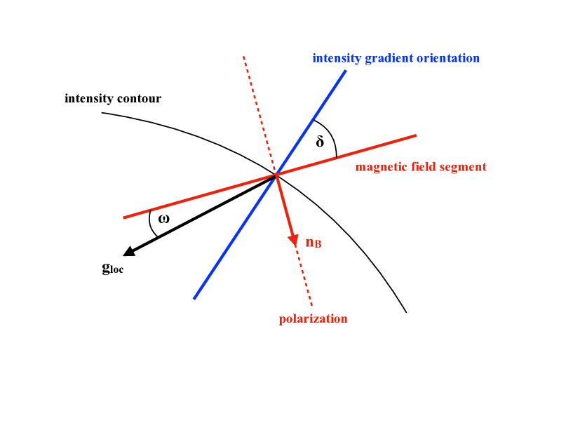
Figure 5: Illustration of relevant angles. $\omega$ measures the deviation between the magnetic field orientation (in the case of submm dust polarization emission rotated by 90^∘ from the originally detected polarization orientation) and the direction of local gravity $\mathbf{g}_{\rm{loc}}$. $\mathbf{n}_{B}$ is the unity vector perpendicular to a measured B-field orientation along the direction of the field tension force. $\delta$ is the angle between a magnetic field orientation and the intensity gradient orientation.

In order to initiate a local collapse, local gravity needs to overcome the magnetic field force and start to bend the field lines. Figure 5 illustrates the geometry adopted from earlier papers (Koch et al., 2012a, 2018). How much gravitational force is available locally to bend and drag a B-field line? This is measured by the projection of the local gravity force $\mathbf{g}_{\rm{loc}}$ onto the direction of the (restoring) field tension $\mathbf{n}_{\rm{B}}$, orthogonal to a B-field line:

$$F_{\rm{loc,c}}\equiv\cos\left(\frac{\pi}{2}-\omega\right)\cdot|\mathbf{g}_{\rm{loc}}|=\sin\omega\cdot|\mathbf{g}_{\rm{loc}}|,$$ (1)

where $F_{\rm{loc,c}}$ is introduced as the net local force (after projection) that can trigger a collapse. Hence, the observed misalignment $\omega(\leq\pi/2)$ between a magnetic field orientation and the local gravity direction quantifies the fraction of the local gravity force that can work to overcome the magnetic field. This fraction is in the range between 0 and 1. The local gravity is directed along a field line with no force component at all to overcome the B-field if $\omega=0$, leading to $F_{\rm{loc,c}}=0$, and the local gravity is maximally working against the B-field if $\omega=\pi/2$ (i.e., local gravity force $\mathbf{g}_{\rm{loc}}$ orthogonal to a B-field orientation, resulting in $F_{\rm{loc,c}}=|\mathbf{g}_{\rm{loc}}|$).

We note that the initial motivation for Equation (1) is different from the $\sin\omega$-measure introduced in Koch et al. (2018). The above equation is motivated by assessing how much of an existing local gravitational pull is effectively directed towards bending and dragging a B-field line, i.e., the local gravitational pull is projected onto the direction of the field tension. In the case of the $\sin\omega$-measure, the B-field tension force is projected onto the local gravity direction in order to measure what fraction of the B-field tension force can impede a gravity-driven motion. In both cases, $\sin\omega$ is quantifying a fraction between 0 and 1, but it is the fraction of the local gravitational pull in the above Equation (1) and the fraction of the B-field tension force in Koch et al. (2018).

4.2.2 Stability and Collapse Criterion

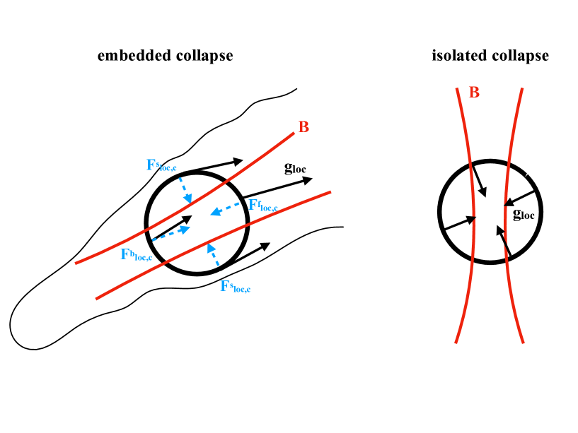
Figure 6: Illustration of the difference between an isolated collapse (right side) and a collapse embedded in a dust lane (left side). The black circles symbolize spherical test volumes to initiate a collapse in the presence of a magnetic field (red lines). The local gravitational field, $\mathbf{g}_{\rm{loc}}$, is shown with black arrows. In the case of the isolated collapse, this vector field is pointing towards the center of the sphere, and the orientation of the magnetic field with respect to this vector field is irrelevant because $\mathbf{g}_{\rm{loc}}$ is azimuthally symmetric. For the embedded collapse, $\mathbf{g}_{\rm{loc}}$ is the result of the surrounding mass distribution. Illustrated is a typical situation as observed in Figure 3, where the local gravitational field along a filamentary dust lane is directed towards the dominating center of mass (in this case towards the right side). Generally, the individual vectors of $\mathbf{g}_{\rm{loc}}$ vary in length (i.e., strength of gravitational pull) and direction. The gravitational pull necessary for an embedded collapse, $F_{\rm{loc,c}}$, is shown with the blue dashed vectors along 4 symbolic directions (front, upper index ’f’; back, upper index ’b’; side, upper index ’s’). Unlike for the isolated case, the relative orientation between field lines and $\mathbf{g}_{\rm{loc}}$ is pivotal because $\mathbf{g}_{\rm{loc}}$ is not azimuthally symmetric. As a consequence, the fraction and magnitude of $\mathbf{g}_{\rm{loc}}$ that is directed towards overcoming the field tension depends on this relative orientation. In particular, for the illustrated configuration, the net available gravitational pull from the sides, $F_{\rm{loc,c}}^{\rm{s}}$ is very small, if $\mathbf{g}_{\rm{loc}}$ and the magnetic field are prevailingly collinear.

From the observed magnetic field morphologies and the gravitational vector field in Figure 3 it is clear that the plane-of-sky projected B-field and local gravity orientations are well aligned in many areas along the dust lanes. If fragmentation and subsequent local collapse are to occur in such a constellation, a local volume needs to become supercritical and decouple from the larger-scale ambient environment in an elongated dust lane. A collapse criterion for an isolated spherically symmetric volume, given by the requirement that the gravitational force dominate over the B-field tension force, $F_{\rm{grav}}>F_{\rm{tension}}$, was given by Schleuning (1998), approximating $F_{\rm{tension}}=1/(4\pi)(\mathbf{B}\cdot\nabla)\mathbf{B}$ as $1/(4\pi)B^{2}/R$ with the magnetic field curvature $1/R$ where $R$ is the field radius. In this hypothetical case of an isolated sphere, the gravitational force field is spherically symmetric and pointing at the center of the sphere. Because of this symmetry, the orientation of an initially uniform or hourglass-like B-field with respect to the spherical volume has no influence on a later collapse. In particular, the local gravity force $\mathbf{g}_{\rm{loc}}$, which can enable collapse, is azimuthally symmetric in this isolated case. This is unlike our observed local field-gravity constellation where $\mathbf{g}_{\rm{loc}}$ has a clear directional dependence and where the magnetic field orientation with respect to the orientation of a dust lane and a possible subsequent collapse makes a decisive difference. Figure 6 schematically illustrates the difference between an isolated collapse and a collapse embedded in a dust lane.

For our observed constellation we can derive a collapse criterion as follows. Along a dust lane we are making the simplifying assumption $F_{\rm{loc,c}}^{\rm{f}}\approx F_{\rm{loc,c}}^{\rm{b}}\approx F_{\rm{loc,c}}$, i.e., the gravitational pull in the front, $F_{\rm{loc,c}}^{\rm{f}}$, is equal to the gravitational pull in the back, $F_{\rm{loc,c}}^{\rm{b}}$. In reality, the pull in the front might be slightly larger due to the smaller $1/r^{2}$ distance term to the dominating centre of gravity (e.g., e2-E in the case of e2). In any case, the directions of both $F_{\rm{loc,c}}^{\rm{f}}$ and $F_{\rm{loc,c}}^{\rm{b}}$ are pointing towards the main centre of gravity which is unlike in the case of the isolated sphere where local gravity from two opposite sides around the sphere is pointing towards the sphere’s centre (Figure 6). The observed constellation clearly seems to favor gas movements along the magnetic field lines along a single direction but not converging to a local center from two opposite sides. The slight difference between $F_{\rm{loc,c}}^{\rm{f}}$ and $F_{\rm{loc,c}}^{\rm{b}}$ might further mean that gas is actually accelerated differentially and stretched, all towards the main gravitating center. This leads to a first conclusion that local gravitational collapse inside a dust lane or extension, if really to happen, will need substantial compression from the side provided by $F_{\rm{loc,c}}^{\rm{s}}$. But this compression from two opposite sides has to overcome a main obstacle, namely the magnetic field tension force (equation (1)). Given the prevailingly close alignment between local gravity and local magnetic field orientation ($\omega$ small), we have $F_{\rm{loc,c}}^{\rm{s}}=\cos(\pi/2-\omega)|\mathbf{g}_{\rm{loc}}|\ll|\mathbf{g}_{\rm{loc}}|$. Hence, a collapse in an extension or dust lane can only be enabled via a radial infall or collapse orthogonal to the local field line. With this and combining with the above expression for the field tension $F_{\rm{tension}}$ by Schleuning (1998), we can write the criterion $F_{\rm{tension}}<F_{\rm{loc,c}}$ which yields

$$B<\sqrt{4\pi R\cdot|\mathbf{g}_{\rm{loc}}|\cdot\sin\omega}.$$ (2)

Adopting Gaussian-base units where $1\rm{G}=1\rm{g}^{1/2}/(\rm{cm}^{1/2}\cdot\rm{s})$, this can be expressed as follows with $B$ in $\rm{G}$ (Gauss):

$$B<9.158\cdot 10^{-4}\cdot\left(\frac{R}{\rm{cm}}\right)^{1/2}\cdot\left(\frac{\sin\omega}{\rm{1}}\right)^{1/2}\cdot\left(\frac{|\mathbf{g}_{\rm{loc}}|}{\rm{g}/(s^{2}\cdot cm^{2})}\right)^{1/2},$$ (3)

where the numerical factor is absorbing the conversion of the gravitational constant to cgs units together with the factor $\sqrt{4\pi}$, and $|\mathbf{g}_{\rm{loc}}|$ also needs to be expressed in cgs units as a gravitational force per volume. Equation (3) can also be written as

$$B<0.1913\cdot\left(\frac{R}{\rm{mpc}}\right)^{1/2}\cdot\left(\frac{\sin\omega}{\rm{1}}\right)^{1/2}\cdot\left(\frac{|\mathbf{g}_{\rm{loc}}|}{\rm{M}_{\odot}\cdot\rm{M}_{\odot}/mpc^{2}}\right)^{1/2},$$ (4)

where $B$ is in $\rm{G}$ (Gauss), and the numerical factor is again absorbing the gravitational constant, the factor $\sqrt{4\pi}$, and the conversion to $\rm{M}_{\odot}$ and $\rm{mpc}$. $|\mathbf{g}_{\rm{loc}}|$ per volume is expressed in $\rm{M}_{\odot}\cdot\rm{M}_{\odot}/mpc^{2}$. For the final source-specific values we use a flux-to-total mass conversion of 2.15 mJy yielding 140 $\rm{M}_{\odot}$ at 1.3 mm with a dust temperature $\rm{T}_{d}=$100 K and a distance of 5.1 kpc.

We note that the criterion in Equation (2) is fundamentally different from a mass-to-flux ratio. The latter one uses a single field strength value to derive a magnetic flux over an area (volume) under consideration. Typically, this is applied to an entire core or cloud, and the magnetic field geometry is not taken into account. Equation (2) is making use of the resolved local magnetic field geometry, which can make a decisive difference as illustrated above with Figure 6. It is the direct comparison of the local direction of gravity versus the local direction of the magnetic field tension force that leads to the criterion in Equation (2) while the mass-to-flux ratio is derived from an average magnetic field strength and an integrated mass.

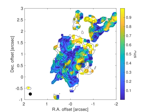
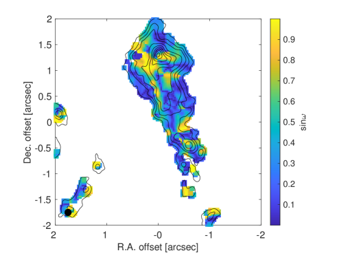
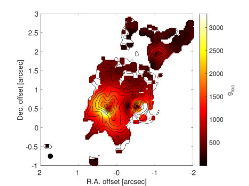
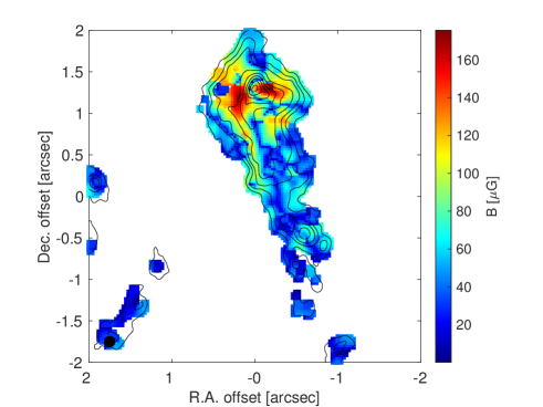
Figure 7: Local magnetic field strength maps (bottom row) derived from the stability and collapse criterion given in equation (2). Separately displayed are the measurable input parameters $\sin\omega$ (top row) and $|\mathbf{g}_{\rm{loc}}|$ (middle row; arbitrary units) for W51 e2 (left column) and e8 (right column).

Equation (2) defines a maximum field strength that can be overcome by an observed field-gravity constellation (the angle $\omega$ is measured and the magnitude of $|\mathbf{g}_{\rm{loc}}|$ can be derived with a dust-to-mass conversion factor), or it defines a minimum field strength that can stabilize a dust lane or extension against a radial collapse. Figure 7 gives a breakdown of equation (2) by separately displaying maps for $\sin\omega$ and $|\mathbf{g}_{\rm{loc}}|$. Field strength limits are of the order of a few tens of $\mu\rm{G}$ in the filamentary dust lanes and extensions, and they grow to about 100-200 $\mu\rm{G}$ in the denser central regions. These field strength limits are smaller than any of the derived values based on dust polarization observations in W51 e2 and e8 (Tang et al., 2009b; Koch et al., 2012a) or from OH maser measurements (Etoka et al., 2012) which are all of the order of a few $\rm{mG}$ up to about 10 $\rm{mG}$. This implies that these resolved filamentary dust lanes and extensions are unlikely to be able to collapse, and therefore, can form accretion channels stabilized by the magnetic field. This is supported by recent results from Goddi et al. (2020) that also find filamentary dust lanes in W51 e2-E and e8 (at 1.3 mm with a resolution of 0$\farcs$02, but without magnetic field detection) which are interpreted as accretion flows.

4.3 Applicability

In this section we address possible complications in the method and criterion introduced in the above sections 4.1 and 4.2. While illustrated specifically with observed quantities for W51 e2 and e8, the following considerations and line of argument remain generally valid.

Opacity. Dust around 230 GHz ($\sim 1.3$ mm) can become optically thick in the very centers of high-mass star-forming regions. Our starting point in section 4.1 was to take an observed dust distribution as a tracer for the distribution of the overall mass. If dust is indeed optically thick in the very center region, this assumption will not hold for that very region as some mass (dust and gas) might be undetected. To be specific, for W51 e2, the recent work by Goddi et al. (2020) finds that dust continuum (observed with ALMA around 1.3mm with a resolution of about 0$\farcs$02) is optically thick up to a radius $\lesssim$ 1000 au in W51 e2-E with a brightness temperature $\gtrsim$ 200 K. This is in agreement with simulations that predict that dust can become optically thick for such central regions (Forgan et al., 2016; Klassen et al., 2016). Depending on opacity, Ginsburg et al. (2017) find a mass of 18 $M_{\odot}$ per beam for the central region in e2-E in the optically thick case ($\tau\geq 1$) and about 6 $M_{\odot}$ per beam in the optically thin case ($\tau\lesssim 1/3$) where one beam refers to their 0$\farcs$2 ALMA observations around 1.3mm. The later estimates in Goddi et al. (2020) with a beam of 0$\farcs$02 are 9.7 $M_{\odot}$ for the central core object in e2-E within a radius of about 500 au, if entirely optically thick, and about 4 $M_{\odot}$ if optically thin. Larger estimates of about 12 $M_{\odot}$ result for lower dust temperatures. Hence, for these two different resolutions, the mass estimates for the central region differ roughly by a factor 2 to 3. These estimates are based on uniform filling factors, and unknown substructures within the beam cannot be accounted for. A similar range in mass estimate is found for the central region covered by one 0$\farcs$2 beam in W51 e8 (Ginsburg et al., 2017). How does this uncertainty in central mass, resulting from these opacity effects, impact our calculation of the gravitational vector field in Figure 3? The effect is likely very minimal for the following reasons. First, the optically thick central areas with a radius 500 to 1000 au (0$\farcs$1 to 0$\farcs$2) are very small compared to the full extension and area ($\sim 3\arcsec\times 3\arcsec$) for both W51 e2 and e8. These central areas are only covering 4 to 16 beams in our observations with a resolution of 0$\farcs$1. Second, the gravitational vector field is calculated taking into account the full area. Since the bulk of the mass is still in the extended area, a factor of 2 to 3 difference in a relatively small mass concentrated in the very center is negligible. In other words, the gravitational effect of this difference is largely diluted over the entire W51 e2 and e8 areas. Third, for both e2 and e8, the gravitational vector field towards and inside the central 0$\farcs$2 area is very radial (Figure 3). A larger or smaller mass concentration (within a factor of a few) will not change the direction of local gravity, because the dust distribution is becoming increasingly circular in the very center, and hence the alignment measure $\sin\omega$ is unaffected. The magnitude of local gravity might change, in a most conservative estimate by a factor of 2 to 3, but more likely by significantly less because it will again be diluted by the distribution of the extended area outside of the very central region.

Outflows. The bottom right panels in Figure 1 and 2 overlay the small-scale collimated SiO outflows (Goddi et al., 2020) and the wider larger-scale ¹²CO outflows (Ginsburg et al., 2017) on our dust continuum and magnetic field detection for W51 e2-E and e8. For e2-E, both outflows are clearly bipolar, they are both along a main southeast-northwest direction, and possibly both outflows have the same origin. W51 e8-N displays a small-scale SiO outflow along an east-west direction and a larger-scale ¹²CO that appears less regular. How far is the presence of these outflows affecting our analysis? Overall, the morphologies in dust and outflows and their spatial locations appear rather different and uncorrelated for both W51 e2 and e8, i.e., the SiO outflow appears only within a central area of about 0$\farcs$4 or less, covering only a small fraction of the area over which the B-field is mapped. Furthermore, the B-field morphology across both the red- and blue-shifted SiO lobe is regular and coherent without any feature that would distinctively delineate a boundary of the SiO outflow. Similarly, no distinct feature in polarization appears at these locations (Figure 12). The mass estimate for the e2-E outflow is $0.36~{}M_{\odot}$ (Goddi et al., 2020), which is negligibly small compared to the central mass and all the extended emission. With a mass of $0.11~{}M_{\odot}$, the same holds for the SiO outflow in e8-N. The ¹²CO outflows are significantly more extended, with the northern lobe in W51 e2 reaching out to e2-NW and the southern lobe extending south far beyond our detected B-field structure, and with both red- and blue-shifted lobes covering most of the mapping area in W51 e8. Analogous to the SiO outflow, the B-field does not show any delineating features between the inside- and outside-outflow areas, but appears coherent and connected across the entire W51 e2 and e8 systems. We note that the brightest contours in the southern ¹²CO lobe in e2-E might fall in between dust lane 1 and 2 (Figure 1, bottom left panel). Similarly, the southern SiO outflow is pointing at the void between dust lane 2 and 3, and the rim of this void shows relatively high polarization fractions (Figure 12). This could indicate that some of the dust lanes are being additionally shaped by the outflows, besides gravity. For a boundary layer between dust lane and outflow, local gravity could then not be calculated as we propose, because the outflowing material will entrain the dust in this layer. However, for the bulk of material inside the dust lane, away from the boundary layer, local gravity can still be calculated as suggested. Moreover, the majority of the dust lanes do not seem to be impacted by the outflows. This finding is consistent with a conclusion in Goddi et al. (2020) where they argue that the dust lanes on a scale of a few thousand au (with a resolution of 0$\farcs$02) are accretion flows and not outflows. Adding that overall both W51 e2 and e8 are gravity-dominated, and generally very little dust is expected to be present in outflow cavities (i.e., dust is likely too weak to be seen), we conclude that the method and criterion in sections 4.1 and 4.2 are applicable in the presence of these outflows. As the magnetic field is stabilizing the dust lanes against collapse, it is at the same time also stabilizing them against any external pressure.

Radiative Feedback. Both thermal and ionizing radiation are expected in high-mass systems. For W51 e2 and e8, Ginsburg et al. (2017) indeed identify chemically enhanced regions as a result of radiative feedback heating the molecular gas. These regions are likely heated by direct infrared radiation from newly forming stars in their centers. With a resolution of $\sim 0\farcs 2$, these heated regions display morphologies that are overall similar to their detected continuum emission, although regions in different molecular lines vary in their sizes from more compact to more extended. This suggests that in these sources on this scale, the dominating effect of this radiative feedback is mostly symmetrical heating and not any disruptive event which would lead to more irregular, disconnected, and broken up morphologies both in these lines and the magnetic field. We note that, e.g., in the presence of expanding HII regions with swept-up shells, the dynamical constellation could be very different. This is observed in the high-mass system G5.89–0.39 which precisely shows swept-up shell morphologies in continuum with a magnetic field aligned with its expanding front (Tang et al., 2009a; Fernández-López et al., 2021). We do not find any indication of such features in W51 e2-E or e8. There might be a hint of a partial shell-like B-field morphology around e2-W, which indeed is harboring an HII region. In this case, dust lane 6 (Figure 1, bottom left panel) might indeed be affected by this feedback, though the polarization coverage is incomplete to be fully conclusive. Hence, we conclude that unless imprints from feedback are clearly visible in continuum and B-field morphology, these systems are still gravity-dominated and our approach remains valid. Radiative heating might further stabilize accreting dust lanes against fragmentation and local collapse. In the case of a dynamically overwhelming feedback, the collapse criterion would need to be expanded with an additional pressure gradient term that can be added to the local gravitational force.

5 Discussion: Towards a Comprehensive Picture from Large-Scale Filamentary Envelope to Core-Accreting Dust Lanes

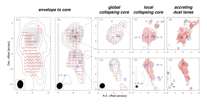
Figure 8: Overview of B-field structures (red segments) in the W51 e2/e8 region with resolutions from about $\theta\sim 3\arcsec$ to $0\farcs 1$, covering scales from about 0.5 pc to 540 au. Contours are dust continuum. Panels from left to right display the distinct regimes as discussed in section 5.1: envelope-to-core scale, global-collapsing-core scale, local-collapsing-core scale, and accreting-dust-lane scale. In panel (a) contours are 3, 6, 10, 20, 30, 40,…$\times\sigma$, where $1\sigma$ is 27 mJy/beam with $\theta\sim 2\farcs 7\times 2\farcs 0$ at a wavelength $\lambda$ around 1.3 mm. Contours are 3, 6, 10, 20, 35, 50, 65, 80, 95,…$\times\sigma$, where $1\sigma$ is 75 mJy/beam with $\theta\sim 2\farcs 13\times 1\farcs 88$ and $\lambda\sim 0.87$ mm in panel (b), 60 mJy/beam with $\theta\sim 0\farcs 7\times 0\farcs 6$ and $\lambda\sim 0.87$ mm in panel (c) and (d), 6 mJy/beam with $\theta\sim 0\farcs 28\times 0\farcs 26$ and $\lambda\sim 1.3$ mm in panel (e) and (f), and 1.2 mJy/beam with $\theta\sim 0\farcs 11\times 0\farcs 10$ and $\lambda\sim 1.3$ mm in panel (g) and (h). Panels (b) to (f) are adapted from Koch et al. (2018).

Combining with earlier data sets, covering physical lengths from about 0.5 pc to 2.6 mpc with resolutions $\theta\sim 3\arcsec$ to $0\farcs 1$ (i.e., going through a range of almost 1,000 in resolved area), we are able to isolate B-field structures in 4 distinct scales and regimes where the B-field is playing different roles. The following sections summarize these different regimes (Figure 8) and diagnostic tools (Figure 9), and discuss their implications. Figure 10 visualizes the evolving role of the B-field across these regimes.

5.1 Distinct Scales: Envelope – Global Collapse – Local Collapse – Core-Connecting Dust Lanes

5.1.1 Envelope-to-Core Scale.

On this largest scale, the W51 e2 and e8 cores are together embedded in a $\sim 0.5$ pc elongated north-south envelope (Figure 8, left and second left panel). The histogram of magnetic field P.A.s (SMA subcompact, $\theta\sim 2\arcsec$; Koch et al., 2018) indicates a prevailing field orientation perpendicular to the envelope’s longer axis. The e2 and e8 cores are aligned perpendicular to this dominating east-west B-field orientation. This B-field-envelope configuration is suggestive of accretion from the east and from the west. Despite a prevailing field orientation, first twists are visible in the B-field morphology (Figure 8, left panel). An analysis based on a local magnetic field dispersion map shows wide areas of very small dispersion indicating and confirming a prevailing B-field orientation, but also a few areas of significant local dispersion. These larger-dispersion areas occur along a southeast-northwest axis in e2 and at the southern end of e8 (Figure 9, left panel). The predictive measure of this analysis on this scale is that these specific locations are pinpointing to where and along which direction the global collapse in e2 and e8 is happening. This defines location and scale of the initial gravitational drag towards the forming e2 and e8 cores. Zooming out, the BIMA observations (Lai et al. (2001); $\theta\sim 3\arcsec$, left panel in Figure 8) possibly probing the outer surface of this envelope, reveal almost uniform B-field orientations along an east-west direction except for the e2 northwestern corner that shows a hint of bent field lines towards e2.

A second important feature on this envelope-to-core scale is the detected bridge between e2 and e8 (around Dec. offset $-3$ in the second panel in Figure 8). While the southern tip of e8 shows a first glimpse of a gravitationally dragged-in B-field morphology, its northern end reveals field lines that are gradually deflecting towards the more massive e2. This clearly different morphology from one end to the other end of the core – as opposed to the symmetrical morphology in the more massive e2 core – is interpreted as local collapse starting at the southern end of e8 while the northern end cannot locally collapse but is being pulled to the more massive e2 core (also see later discussion in section 5.2 and Figure 11). This particular feature is analyzed in a forthcoming work that investigates gravitational entrainment of the B-field in order to derive a field strength estimate (Koch et al., in preparation).

5.1.2 Global-Collapsing-Core Scale.

On this $\sim 0.05$pc scale the e2 and e8 cores are clearly detected as entities, the surrounding larger-scale diffuse envelope is resolved out, and in particular e2 shows an hourglass-type B-field morphology towards its dominating gravitational center. The field lines are clearly bent and almost radial-like (SMA extended, $\theta\sim 0\farcs 7$; Tang et al., 2009b). The B-field detection in e8 is less complete though also hinting collapse with field orientations directed towards the main center in e8 (Figure 8, middle panels). With the introduction of the angle $\delta$ as an observable and diagnostic tool , the polarization–intensity gradient method leads to a $\Sigma_{\rm{B}}$-map for e2 with values around 0.2 to 0.3 across the entire core. $\Sigma_{\rm{B}}$ values below 1, i.e., a magnetic field tension-to-gravity force ratio below 1, indicate that gravity is overwhelming the B-field in this area. The e2 core, as an entity, can thus engage in a global collapse (Figure 9, second left panels). It is only the northwestern extension where $\Sigma_{\rm{B}}$ is larger than 1 or around 1. Here, the B-field is strong enough to dominate over gravity and halt any infall or collapse motion. Looking at the radial profile of $\Sigma_{\rm{B}}$ there is an obvious drop from values around 0.8 at the periphery of the core to values of 0.2 in the center of the core. Consequently, the magnetic field in the observed configuration is leading to a gravity dilution on the global-collapsing-core scale, i.e., a gravity efficiency smaller than 1, quantified by $\Sigma_{\rm{B}}$. Gravity is only about 20% effective in the core’s periphery while quickly increasing to around 80% in the inner core as compared to free-fall enabled by gravity exclusively (Figure 4 in Koch et al., 2012b). In an analogous way, the profile of mass-to-flux ratio, independently derived from $\Sigma_{\rm{B}}$, shows a transition from subcritical at larger radius to supercritical within the core (Figure 6 in Koch et al., 2012b). The magnetic field strength map, derived with the polarization–intensity gradient method, displays a field strength $B$ growing from the periphery to the center, reaching around 19 mG in the center with a radial profile close to $B(r)\sim r^{-1/2}$. It is evident from this analysis that the magnetic field properties are not constant across the core, but vary substantially in defining the role of the magnetic field (Figure 9, second left panels). It is interesting to note that the orientation of the e2 core with its northwestern extension is clearly reflected with the axis of larger B-field dispersion values (on the envelope-to-core scale) as noted above in section 5.1.1.

We remark that identical trends, as seen in $\Sigma_{\rm{B}}$ and mass-to-flux ratio on this global-collapsing-core scale, are also seen on zoomed-out larger scales, namely a field-to-gravity force ratio $\Sigma_{\rm{B}}$ being largest in between e2 and e8 with values dropping towards both cores, and again on an even further zoomed-out scale, $\Sigma_{\rm{B}}$ being largest in between W51 North and W51 e2/e8 together with values dropping towards the W51 e2/e8 complex and the W51 North complex (Koch et al., 2012b). This suggests a self-similar collapse picture, or multi-scale collapse-within-collapse scenario as discussed further in section 5.2.

5.1.3 Local-Collapsing-Core Scale.

Zooming in on e2 and e8 reveals detailed substructures below the above global-collapsing-core scale in section 5.1.2. The cores fragment into smaller cores and with that generic B-field morphologies are detected (Koch et al., 2018). The previous hourglass-type global-collapse signature is resolved into smaller-scale features reflecting local and inter-core dynamics imprinted onto the B-field morphology (Figure 8, second right panels). In particular, satellite cores with a bow-shock shaped field structure are seen in e2-NW and e8-S. They both appear to fall into or merge with their bigger neighboring cores, e2-E/e2-W and e8-N, respectively. From two sides centrally converging B-field structures are visible along a northwest direction from e2-E and in between e8-S and e8-N. Several cores reveal a prominent B-field asymmetry – gravitationally bent and dragged-in B-field morphology in one half of a core with compressed, straightened and deflected field lines in the other half of the core – suggestive of local collapse happening on one end while the core itself is pulled towards the next bigger more massive neighboring core. This is seen in e2-NW being pulled towards e2-E/e2-W, and e8-S being pulled towards e8-N.

This locally varying role of the B-field, specifically focusing on the inter-core and converging field structures, is reflected in the $\sin\omega$ measure. $\sin\omega$ in the range between 0 and 1 measures the fraction of the local magnetic field tension force that can work against local gravity. The asymmetrical B-field structure in these locally collapsing cores is captured with $\sin\omega$ values around 0 on the collapsing sides and with maximum $\sin\omega$ values close to 1 on the sides being pulled to the next larger collapse centers (Figure 9, second right panels). Thus, on this local-collapse and inter-core scale the role of the B-field can flip from essentially no resistance to maximum resistance against collapse. Similarly, low $\sin\omega$ values across the global e2 and e8 cores localize regions where gravity is unobstructed. These regions were suggested to represent magnetic channels in Koch et al. (2018).

5.1.4 Accreting-Dust-Lane Scale.

Moving to a $0\farcs 1$ resolution ($\sim 540$ au) seems to resolve a critical physical length scale around the W51 e2 and e8 core in such that we start to witness the departure from near-spherical structures and resolve a network of filamentary dust lanes and extensions (Figure 1, 2, and right panels in Figure 8). As described in the above sections 4.1 and 4.2, the observed characteristics on this scale are (1) a B-field prevailingly aligned with dust lanes, and (2) local gravity mostly directed along dust lanes towards the central mass concentration. Given this observed morphology, section 4.2 is investigating the B-field-induced stability against a radial collapse in these dust lanes. Since it is found that small field strength values are already sufficient to balance local gravity (these values are smaller than previously derived and observed values), it is unlikely that these structures further fragment and collapse. This leads to the conclusion that the magnetic field is playing a decisive role in stabilizing these structures. Based on this, we propose that these observed dust lanes represent stable accretion zones and channels towards the denser core regions where material is guided by magnetic fields. Adding the magnetic field into this picture complements recent results by Goddi et al. (2020) who interpret the filamentary dust lanes arising from the compact cores in W51 e2-E, e8, and North as multidirectional mass accretion. If indeed present, these accretion streams can provide a mechanism to feed 100-au-scale or smaller Keplerian disks. Such a mechanism can be of interest because the formation of large and stable 1000-au-scale disks in high-mass star-forming systems can be challenging (e.g., Rosen et al., 2019; Seifried et al., 2015; Myers et al., 2013; Commerçon et al., 2011). Further support for such a scenario comes from the numerical work by Mignon-Risse et al. (2021) who find filamentary structures linking to magnetically regulated $\sim$100 to 200-au disks. These structures, referred to as streamers, are identified as a path for accretion flows where the magnetic field is pulled along, and the gas moves along the field lines. Their accretion streamers are thermally dominated and magnetically stabilized.

Recent work on the Serpens South region has also found a parallel B-field alignment in one filament that is interpreted as evidence for gravity dragging the denser gas, in this case derived in the context of a change of alignment as compared to lower visual extinction areas, and entraining the flux-frozen large-scale B-field (Pillai et al., 2020). Calculating the actual gravitational vector field (Figure 3) adds an important observable and strongly corroborates this picture in W51 e2 and e8. The $\sin\omega$ maps (top row in Figure 7) further substantiate this, clearly displaying very small values towards all cores. As $\sin\omega$ is a measure for the magnetic field’s efficiency to oppose gravity, its small values naturally are consistent with a gravity-induced alignment where gravity can entrain the B-field and form channels where material is preferentially moving and accreting along the B-field lines towards a central denser region. This is precisely the scenario put forward in Wang et al. (2020) for the G$33.92+0.11$ hub-filament system based on a detailed analysis of local correlations between magnetic field, gravity, and velocity gradients, and it is identical with the cartoon in Busquet (2020) illustrating the alignment transition discussed in Pillai et al. (2020) at visual extinctions $A_{v}\gtrsim 21$. In summary, the quantitative analysis here based on $\sin\omega$, $|\mathbf{g}_{\rm{loc}}|$, and the B-field’s stabilizing role (Figure 7) is suggestive of an emerging picture where the detected dust lanes form fundamental accretion regions and channels where gravity and B-field are prevailingly aligned with these structures. The dust lanes are likely gravitationally driven, seen in an underlying gravitational skeleton (Figure 4) and magnetically stabilized. Such structures have been found in various simulations investigating the evolution of molecular clouds and accretion onto denser structures (Körtgen & Banerjee, 2015; Gómez et al., 2018; Li et al., 2018).

5.2 Self-Similarity and Multi-Scale Embedded Collapse: Imprint onto B-field Morphology and Gravitational Field

The previous section has described four distinct scales with four distinct physical regimes where the role of the magnetic field is quantified with various novel measures. Identifying these distinct scales is the result of a series of observations with successively higher resolutions. With these higher interferometric resolutions more and more of the surrounding diffuser emission is stepwise resolved out. Hence, the gradually higher resolutions are probing more and more of the inner and denser regions. Patching this together leads to a picture from a pc-scale encompassing envelope to mpc-scale core-accreting dust lanes.

Here, we emphasize one particular aspect in this picture, namely the repeating structures in the magnetic field morphology and the gravitational vector field across different scales. This is most evident when comparing the envelope-to-core scale and the local-collapsing-core scale as highlighted in Figure 11. The W51 e2/e8 complex has its dominating mass centered on e2. As a consequence, on the envelope-to-core scale, e2 displays the beginning of a global collapse (i.e., a collapse of the entire e2 core as an entity) with clearly bent field lines in its northwestern and southeastern zones. Differently, the less massive e8 core shows the beginning of pulled-in field lines on only one end, namely in its south. At the northern end, the field lines appear to be bending away, from straight east-west-oriented lines around offset Dec. $\sim-5\arcsec$, and turning to be more redirected towards the center of e2 (Figure 11, top left panel). On a smaller scale, inside the global collapse of e2 and e8, the magnetic field morphologies in e8-S, e2-W, and e2-NW show a similar structure, i.e., bent and likely gravitationally pulled-in field lines on one end (southern end in e8-S, western end in e2-W, western end in e2-NW) and straightened, opened up, and redirected lines on the other end (northern end in e8-S, eastern side in e2-W, eastern/south-eastern side in e2-NW; top right panels in Figure 11). An analogous picture is seen in the gravitational vector field (bottom panels in Figure 11). Section 4.1 has described the trend of the local gravitational field converging towards the local peak emission on one side of a core while the other side is revealing local gravity to be pointing away towards the neighboring dominating mass concentration. This is seen for e8-S towards e8-N, e2-W towards e2-E, and e2-NW towards e2-E/e2-W. An identical pattern in the gravitational vector field, on a larger scale, is observed between e8 (as an entity) and the northern more massive e2 (as an entity). In short, these observations show self-similar structures in magnetic field and gravitational vector field on scales of 0.5 pc and 0.05 pc. This local collapse happening simultaneously with the global collapse points at a collapse-within-collapse scenario.

Recent numerical works by Gómez et al. (2018); Vázquez-Semadeni et al. (2019) suggest a multi-scale, global hierarchical collapse scenario, described as a flow regime of collapses within collapses. This matches very well our multi-scale observational findings of B-field morphologies and gravitational field. In the global hierarchical collapse by Vázquez-Semadeni et al. (2019), all scales accrete material from their parent structures and filamentary accretion is a natural consequence of gravitational collapse.

Finally, we note that zooming out to an even larger scale – encompassing the W51 e2/e8 complex and the W51 North complex – a self-similar structure is also present (Figure 1 in Koch et al., 2012b). An analysis of the magnetic field tension-to-gravity force ratio $\Sigma_{\rm{B}}$ shows the largest values above one in between the two complexes with ratios systematically decreasing and falling below one towards both complexes. The same trend in $\Sigma_{\rm{B}}$ is then also seen with higher-resolution observations for W51e2 and e8 and further within e2 (Koch et al., 2012b). Therefore, we argue that all together the W51 region is displaying self-similar multi-scale collapse features across three different scales.

6 Summary and Conclusion

We are presenting ALMA continuum polarization observations towards the high-mass star-forming regions W51 e2 and e8 in Band 6 (around 230 GHz; $\lambda\sim$1.3 mm) with a resolution of $0\farcs 1$ which corresponds to about 540 au. Together with earlier observations we are proposing a multi-scale synergetic scenario for the different roles of the magnetic field from the large-scale 0.5 pc envelope to core-connecting networks of dust lanes with widths of a few 100 au. Our main results are summarized in the following.

1. Polarization Detection. Polarized emission at a resolution of about 540 au is clearly detected in W51 e2 and e8. Polarization percentages range from about 0.1% to about 15%, with averages around 3%. A typical anti-correlation between polarization percentage and Stokes $I$ is observed, though with a large scatter and shallower slopes (around $-0.8$) than in coarser observations in the same source.

2. New Structural Features. These latest observations mark a departure from spherical and elongated structures seen in earlier observations. A connecting network of filamentary dust lanes is resolved in continuum with widths around 540 au to 2,000 au. These dust lanes are located in the periphery of cores and in between cores. The cores do not appear to fragment further. Magnetic field structures are resolved in dust lanes and extensions. A transition from perpendicular field lines in the surrounding diffuser region to field lines aligning with the denser central spine in the connecting extension between cores is observed in e8. Three sectors in the inner $0\farcs 5$ region around e2-E display nearly straight field lines that are rotated by $90^{\circ}$ from one sector to the next. These lines abruptly change orientation towards the innermost center, forming a northwest-southeast aligned structure, possibly hinting the presence of a small disk close to where a small-scale collimated SiO outflow is seen.

3. Gravitational Field and Magnetic Field Morphology. The magnetic field orientations are prevailingly aligned parallel to the dust lanes. At the same time, the gravitational vector field is typically also along the dust lanes, while additionally hinting a gravitational skeleton that defines ridges which likely form the underlying structures of the dust lanes. Hence, B-field and gravitational field show a very similar overall configuration. This implies that gravitational pull is mostly directed along B-field lines. A noticeably distinct feature in the gravitational field is the converging vector field on one side of a core with the gravitational vector field on the other side of the core being gradually redirected towards the neighboring more massive core.

4. Local Collapse Criterion and B-field-Induced Stability. Utilizing the detected magneto-gravitational field configuration, a local stability and collapse criterion is derived. This criterion is based on the measurable magnitude of local gravity and the measurable angle between the local orientations of gravity and magnetic field. The criterion sets a limit to the maximum local magnetic field strength that can be overcome with an observed magneto-gravitational field configuration, or in other words, it defines the necessary minimum field strength to prevent a local collapse. The resulting field strengths suggest that the filamentary dust lanes and extensions are stable, possibly forming a fundamental structure in the accretion of material towards central sources and disks. The magnetic field can stabilize the dust lanes both against a local collapse and also against external pressure.

5. Synergetic Picture and Multi-Scale Collapse. Combining resolutions starting from pc-scale to the latest mpc-scale, four distinct scales can be identified in the W51 region: envelope-to-core scale, global-collapsing-core scale, local-collapsing-core scale, accreting-dust-lane scale. The roles of the magnetic field differ with these scales. Various diagnostic tools are summarized to quantify the different roles. Repeating structures in the B-field morphology and the gravitational field are seen on different scales. These self-similar structures suggest a multi-scale collapse-within-collapse scenario. This starts from scales of several pc until the eventual emergence of a network of stable core-connecting and accreting dust lanes on mpc scale where gravity and magnetic field are all aligned with the dust lanes, suggestive of a gravity-entrained alignment. Hence, the dust lanes are likely gravitationally driven and magnetically stabilized.

Appendix: Polarization Properties

The basic polarization characteristics are displayed in the Figures 12 and 13. Typical trends are observed, namely a generally growing polarized signal $I_{p}$ towards the dust continuum peaks with a generally decreasing polarization percentage $p=I_{p}/I$. We note that the peaks in $I_{p}$ are offset from the Stokes $I$ peaks, both in e2 and e8, and e2 appears to have two peaks with one to the east and one to the west (Figure 12). While the common anti-correlation $p$ versus $I$ is seen, the large vertical scatter of about one order of magnitude indicates that there are likely more complicated physical processes ongoing which are not captured with this simple anti-correlation. The slopes for the best-fit power laws are slightly different for e2 ($-0.81$) and e8 ($-0.77$). They appear to be shallower than the ones derived from the coarser observations at the same frequency ($\theta\sim 0\farcs 26$, 230 GHz; Koch et al. (2018)) which yielded $-1.02$ and $-0.84$ for e2 and e8, respectively. Polarization percentages with maxima, minima, and standard deviations (Figure 13) are similar to the values from the coarser observations.

Figure 9: Overview of diagnostic tools in the W51 e2/e8 region. From left to right, on the envelope-to-core scale the local magnetic field dispersion can pick out location and direction where a global collapse will start to happen (zones with larger dispersion values); on the global-collapsing-core scale, the small values of the magnetic field tension-to-gravity force ratio $\Sigma_{\rm{B}}$ across the core indicate that e2 as an entity can globally collapse (upper panel), and the measured magnetic field strength map reveals a clearly growing strength towards the center (lower panel); on the local-collapsing-core scale, the $\sin\omega$ measure locates regions where gravity is unobstructed (small values) and where the B-field can maximally slow down gravity (values close to one) towards locally collapsing smaller cores; on the accreting-dust-lane scale (rightmost panels), ridges formed by the locally converging gravitational field (gray arrows) appear in areas labelled as dust lanes in Figure 1 and 2, which typically also coincide with small angles $\omega$ (color scale). Low $\sin\omega$ values on the local-collapsing-core scale are signposts of the appearance of dust lanes at higher resolutions. Panels in the first three columns are adapted from Koch et al. (2012a) and Koch et al. (2018).

Figure 10: Visualization of the evolving roles of the magnetic field over the scales presented in Figures 8 and 9. Visualized are streamlines based on the detected magnetic field morphologies in Figure 8 using a line convolution algorithm for vector fields (e.g., Cabral & Leedom (1993)). From left to right are envelope-to-core scale (first and second), global-collapsing-core scale (third), local-collapsing-core scale (forth), and accreting-dust-lane scale (fifth). No visualization is shown in black patches with too sparse sampling in the original data which does not allow to construct a connected convolution.

Figure 11: Self-similar structures on two different scales (envelope-to-core scale (section 5.1.1; left column) and local-collapsing-core scale (section 5.1.3; right column) in their detected magnetic field morphologies (red segments, top row) and their gravitational vector fields (black arrows, bottom row). Green boxes mark the self-similar structures. On the envelope-to-core scale between e8 and e2, the gravitational field starts to be deflected in the north of e8, gradually pointing more towards e2. The more massive e2 core mostly displays an azimuthally symmetric gravitational field. This systematic deflection towards the more massive local center is seen again on smaller scales when zooming in between the cores e2-W and e2-E, e2-NW and e2-E/e2-W, and e8-S and e8-N. The B-field morphology shows a characteristic feature where the field segments are bent away from the less massive core and straightened towards the more massive local center. These recurring structures point at a multi-scale collapse-within-collapse scenario which leaves its imprints both in the B-field and the gravitational vector field.

Facilities: ALMA.

References

- Andersson et al. (2015) Andersson, B.-G., Lazarian, A., & Vaillancourt, J. E. 2015, ARA&A, 53, 501
- Añez-López et al. (2021) Añez-López, N., Busquet, G., Koch, P.M. et al. 2020, A&A, 644A, 52A
- Arzoumanian et al. (2021) Arzoumanian, D., et al. 2021, A&A, 647, A78
- Beltrán et al. (2019) Beltrán, M.T. et al. 2019, A&A, 630, A54
- Busquet (2020) Busquet, G., 2020, Nat. Astron., 4, 1126
- Cabral & Leedom (1993) Cabral, B. & Leedom L. C. 1993 Proc. XX Annual Conf. Computer Graphics and Interactive Techniques, SIGGRAPH ’93 (New York: Association for Computing Machinery) 263
- Cho & Lazarian (2005) Cho, J., Lazarian, A. 2005, ApJ, 631, 361
- Commerçon et al. (2011) Commerçon, B., Hennebelle, P., & Henning, T. 2011, ApJL, 742, L9
- Cortes et al. (2016) Cortes, P. et al. 2016, ApJ, 825, L15
- Crutcher (2012) Crutcher, R.M. 2012, ARA&A, 50, 29
- Cudlip et al. (1982) Cudlip, W., Fruniss, I., King, K. J., & Jennings, R. E. 1982, MNRAS, 200, 1169
- Draine & Weingartner (1996) Draine, B.T., & Weingartner, J.C. 1996, ApJ, 470, 551
- Draine & Weingartner (1997) Draine, B.T., & Weingartner, J.C. 1997, ApJ, 480, 633
- Etoka et al. (2012) Etoka, S., Gray, M.D., Fuller, G.A. 2012, MNRAS, 423, 647
- Fernández-López et al. (2021) Fernández-López, M., et al. 2021, ApJ, 913, 29F
- Fissel et al. (2016) Fissel, L.M. et al. 2016, ApJ, 824, 134
- Forgan et al. (2016) Forgan, D.H., Idee, J.D., Cyganowski, C.J., Brogan, C.L., & Hunter, T.R. 2016, MNRAS, 463, 957
- Ginsburg et al. (2015) Ginsburg, A. et al. 2015, A&A, 573, A106
- Ginsburg et al. (2017) Ginsburg, A., Goddi, C., Diederik Kruijssen, J.M., et al. 2017, ApJ, 842, 92
- Goddi et al. (2020) Goddi, C., Ginsburg, A., Maud, L.T., et al. 2020, ApJ, 905, 25
- Gómez et al. (2018) Gómez, G.C., Vázquez-Semadeni, E., & Zamora-Avilés, M. 2018, MNRAS, 480, 2939
- Hennebelle & Inutsuka (2019) Hennebelle, P & Inutsuka, S.-i., 2019, Frontiers in Astronomy and Space Sciences, 6, 5
- Hildebrand (1988) Hildebrand, R. H. 1988, QJRAS, 29, 327
- Hildebrand et al. (1984) Hildebrand, R. H., Dragovan, M., & Novak, G. 1984, ApJ, 284, L51
- Hoang & Lazarian (2016) Hoang, T., & Lazarian, A. 2016, ApJ, 831, 159H
- Klassen et al. (2016) Klassen, M., Pudritz, R.E., Kuiper, R, Peters, T., & Banerjee, R. 2016, ApJ, 823, 28
- Koch et al. (2010) Koch, P.M., Tang, Y.-W., Ho, P.T.P. 2010, ApJ, 721, 815
- Koch et al. (2012a) Koch, P.M., Tang, Y.-W., Ho, P.T.P. 2012a, ApJ, 747, 79
- Koch et al. (2012b) Koch, P.M., Tang, Y.-W., Ho, P.T.P. 2012b, ApJ, 747, 80
- Koch et al. (2013) Koch, P.M., Tang, Y.-W., Ho, P.T.P. 2013, ApJ, 775, 77K
- Koch et al. (2014) Koch, P.M., Tang, Y.-W., Ho, P.T.P. , Zhang, Q., Girart, J.M., Chen, H.-R.V. et al. 2014 ApJ, 797, 99
- Koch et al. (2018) Koch, P.M., Tang, Y.-W., Ho, P.T.P. , Yen, H.-W., Su, Y.-N., and Takakuwa, S. 2018, ApJ, 855, 39
- Körtgen & Banerjee (2015) Körtgen, B. & Banerjee, R. 2015, MNRAS, 451, 3340
- Lai et al. (2001) Lai, S.-P., Crutcher, R.M., Girart, J.M., Rao, R. 2001, ApJ, 561, 864L
- Lazarian (2000) Lazarian, A. 2000, ASPC, 215, 69
- Lazarian & Hoang (2007) Lazarian, A., & Hoang, T. 2007, MNRAS, 378, 910
- Leahy (1989) Leahy, P. 1989, VLA Scientific Memoranda 161 (Socorro, NM: VLA)
- Li et al. (2014) Li, H.-B. et al. 2014, Protostars and Planets VI (eds. Beuther, H. et al.) 101-123 (Univ. of Arizona Press, 2014)
- Li et al. (2018) Li, P.-S., Klein, R.I., & McKee, C.F. 2018, MNRAS, 473, 4220
- Nagai et al. (2016) Nagai, H., Nakanishi, K., Paladino, R. et al. 2016, ApJ, 824, 132
- Mignon-Risse et al. (2021) Mignon-Risse, R., González, M., Commerçon, B., & Rosdahl, J. 2021, A&A, 652, A69
- Myers et al. (2013) Myers, A.T., McKee, C.F., Cunningham, A.J., Klein, R.I., & Krumholz, M.R. 2013, ApJ, 766, 97
- Palau et al. (2021) Palau, A. et al. 2021, ApJ, 912, 159P
- Pillai et al. (2020) Pillai, T.G.S., Clemens, D.P., Reissl, S. et al. 2020, Nat. Astron., 4, 1195
- Planck Intermediate Results XIX (2015) Planck Intermediate Results XIX, 2015, A&A, 576, A104
- Planck Intermediate Results XX (2015) Planck Intermediate Results XX, 2015, A&A, 576, A105
- Rosen et al. (2019) Rosen, A.L., Li. P.S., Zhang, Q., & Burkhardt B. 2019, ApJ, 887, 108
- Saral et al. (2017) Saral, G. et al. 2017, ApJ, 839, 108
- Sato et al. (2010) Sato, M., Reid, M.J., Brunthaler, A., & Menten, K.M. 2010, ApJ, 720, 1055
- Schleuning (1998) Schleuning, D.A. 1998, ApJ, 493, 811
- Seifried et al. (2015) Seifried, D., Banerjee, R., Pudritz, R.E., & Klessen, R.S. 2015, MNRAS, 446, 2776
- Shi et al. (2010) Shi, H., Zhao, J.-H., & Han, J.L., 2010a, ApJ, 718, L181
- Soam et al. (2019) Soam, A. et al. 2019, ApJ, 883, 95
- Takahashi et al. (2019) Takahashi, S., et al. 2019, ApJ, 872, 70
- Tang et al. (2009a) Tang, Y.-W., Ho, P.T.P., Girart, J.M., Rao, R., Koch, P.M., Lai, S.-P. 2009a, ApJ, 695, 1399
- Tang et al. (2009b) Tang, Y.-W., Ho, P.T.P., Koch, P.M., Girart, J.M., Lai, S.-P., Rao, R. 2009b, ApJ, 700, 251
- Tang et al. (2013) Tang, Y.-W. , Ho, P.T.P., Koch, P.M., Guilloteau, S. & Dutrey, A. 2013, ApJ, 763, 135
- Tang et al. (2019) Tang, Y.-W., Koch, P.M., Peretto, N. et al. 2019, ApJ, 878, 10
- Vázquez-Semadeni et al. (2019) Vázquez-Semadeni, E., Palau, A., Ballesteros-Paredes, J., Gómez, G.C., & Zamora-Avilés, M. 2019, MNRAS, 490, 3061
- Wang et al. (2020) Wang, J.-W., Koch, P.M., Galván-Madrid, R. et al. 2020, ApJ, 905, 158
- Wardle & Kronberg (1974) Wardle, J. F. C. & Kronberg, P. P. 1974, ApJ, 194, 249
- Xu et al. (2009) Xu, Y., Reid, M.J., Menten, K.M., Brunthaler, A., Xheng, X.W., & Moscadelli, L. 2009, ApJ, 693, 413
- Zhang et al. (2014) Zhang, Q., Qiu, K., Girart, J.M., Liu, H.-Y.B., Tang, Y.-W., Koch, P.M., et al., 2014, ApJ, 779, 116