Inverse Problems for Subdiffusion from Observation at an Unknown Terminal Time

Abstract

Inverse problems of recovering space-dependent parameters, e.g., initial condition, space-dependent source or potential coefficient, in a subdiffusion model from the terminal observation have been extensively studied in recent years. However, all existing studies have assumed that the terminal time at which one takes the observation is exactly known. In this work, we present uniqueness and stability results for three canonical inverse problems, e.g., backward problem, inverse source and inverse potential problems, from the terminal observation at an unknown time. The subdiffusive nature of the problem indicates that one can simultaneously determine the terminal time and space-dependent parameter. The analysis is based on explicit solution representations, asymptotic behavior of the Mittag-Leffler function, and mild regularity conditions on the problem data. Further, we present several one- and two-dimensional numerical experiments to illustrate the feasibility of the approach.
Key words: backward subdiffusion, inverse source problem, inverse potential problem, subdiffusion, unknown terminal time

1 Introduction

Let $\Omega\subset\mathbb{R}^{d}$ ($d=1,2,3$) be an open bounded smooth domain with a boundary $\partial\Omega$. Consider the following initial-boundary value problem with $\alpha\in(0,1)$ for the subdiffusion model:

$$\left\{\begin{aligned} \partial_{t}^{\alpha}u-\Delta u+qu&=f,&&\mbox{in }\Omega\times(0,\infty),\\ u&=0,&&\mbox{on }\partial\Omega\times(0,\infty),\\ u(0)&=u_{0},&&\mbox{in }\Omega,\end{aligned}\right.$$ (1.1)

where $T>0$ is a fixed final time, $f\in L^{\infty}(0,T;L^{2}(\Omega))$ and $u_{0}\in L^{2}(\Omega)$ are given source term and initial data, respectively, the nonnegative function $q\in L^{\infty}(\Omega)$ is a spatially dependent potential, and $\Delta$ denotes the Laplace operator in space. The notation ${\partial^{\alpha}_{t}}u(t)$ denotes the Djrbashian-Caputo fractional derivative in time $t$ of order $\alpha\in(0,1)$ ([10, p. 70] or [4, Section 2.3.2])

$${\partial^{\alpha}_{t}}u(t)=\frac{1}{\Gamma(1-\alpha)}\int_{0}^{t}(t-s)^{-\alpha}u^{\prime}(s)\mathrm{d}s,$$ (1.2)

where $\Gamma(z)$ is the Gamma function defined by $\Gamma(z)=\int_{0}^{\infty}s^{z-1}e^{-s}\mathrm{d}s$, for $\Re(z)>0$. Note that the fractional derivative ${\partial^{\alpha}_{t}}u$ recovers the usual first-order derivative $u^{\prime}(t)$ as $\alpha\to 1^{-}$ if $u$ is sufficiently smooth. Thus the model (1.1) can be viewed as a fractional analogue of the classical parabolic equation.

The model (1.1) arises naturally in the study of anomalously slow diffusion processes, which encompasses a broad range of important applications in engineering, physics and biology. The list of successful applications include thermal diffusion in fractal media [21], dispersion in heterogeneous aquifer [1], ion dispersion in column experiments [2], and protein transport in membranes [11], to name just a few. Thus its mathematical theory has received immense attention in recent years; see the monographs [12, 4] for detailed discussions on the solution theory. Related inverse problems have also been extensively studied [7, 17, 15]. The surveys [17] and [15] cover many inverse source problems and coefficient identification problems, respectively.

The observation $g(x)=u(x,T)$, $x\in\Omega$, at a terminal time $T$ is a popular choice for the measurement data in practice. There is a very extensive literature on inverse problems using terminal data, e.g., backward sudiffusion [22, 28], inverse source problem [7, 17, 3], and inverse potential problem [27, 9, 8, 26], where the references are rather incomplete but we refer to the reviews [7, 17, 15] for further references. Notably, several uniqueness and stability results have been proved. For example, backward subdiffusion is only mildly ill-posed, and enjoys (conditional) Lipschitz stability [22, Theorem 4.1], cf. (2.9) below. In all these existing studies, the terminal time $T$ at which one collects the measurement has always been assumed to be fully known. Nonetheless, in practice, the terminal time $T$ might be known only imprecisely. Therefore, it is natural to ask whether one can still recover some information about the concerned parameter(s). The missing knowledge of $T$ introduces additional challenges since the associated forward map is not fully known then. In this work, we address this question in the affirmative both theoretically and numerically, and study the inverse problem of identifying one of the following three parameters: (i) initial condition $u_{0}$, (ii) space-dependent source component $\psi$, and (iii) space-dependent potential $q$, from the observation $u(T)$ at an unknown terminal time $T$.

For each inverse problem, we shall establish the unique recovery of the space-dependent parameter and the terminal time $T$ simultaneously from the terminal observation, as well as conditional stability estimates, under suitable a priori regularity assumptions on the initial data $u_{0}$ and the source $f$; see Theorems 2.2, 3.2 and 4.3 for the precise statements. The analysis relies heavily on explicit solution representations via Mittag-Leffler functions (see, e.g., [22], [4, Section 6.2]). The essence of the argument is that the regularity difference leads to distinct decay behavior of the Fourier coefficients of $u_{0}$ and $f$. This combined with distinct polynomial decay behaviour of Mittag–Leffler function $E_{\alpha,1}(z)$ (on the negative real axis) allows uniquely determining the terminal time $T$. Note that the polynomial decay holds only for $E_{\alpha,1}(z)$ with a order $\alpha\in(0,1)$, and does not hold in the integer case (i.e., $\alpha=1)$. Thus, the unique determination of $T$ does not hold for normal diffusion. Once the terminal time $T$ is determined, the unique determination of the space-dependent parameter follows. The proof of the stability results relies on smoothing properties of the solution operators. In addition, we present several numerical experiments to illustrate the feasibility of numerical recovery. The numerical reconstructions are obtained using the Levenberg-Marquadt method [13, 19]. Numerically, by choosing the hyperparameters in the method properly, both space-dependent parameter and terminal time can be accurately recovered. To the best of our knowledge, this work presents the first uniqueness and stability results for inverse problems from terminal data at an unknown time.

The rest of the paper is organized as follows. In Section 2, we present uniqueness and stability results for the backward problem, which are then extended to the inverse source problem in Section 3. In Section 4, we discuss the inverse potential problem, which requires several new technical estimates on the solution regularity and asymptotic decay. Finally, some numerical results for one- and two-dimensional problems are given in Section 5. Throughout, we denote by $u=u(v)$ and $\tilde{u}=u(\tilde{v})$ the solutions to problem (1.1) with the space dependent parameter $v$ and $\tilde{v}$, respectively. We often write a function $f(x,t):\Omega\times(0,T)\to\mathbb{R}$ as $f(t)$ a vector-valued function on $(0,T)$. The notation $c$ denotes a generic constant which may differ at each occurrence, but it is always independent of the concerned parameter and terminal time $T$.

2 Backward problem

In this section, we investigate the backward problem (BP): recover the initial data $u_{0}=u(0)$ from the solution profile $u(T)$ to problem (1.1) at an unknown terminal time $T$.

2.1 Solution representation

First we recall the solution representation for problem (1.1), which plays a key role in the analysis below. For any $s\geq 0$, we denote by $\dot{H}^{s}(\Omega)\subset L^{2}(\Omega)$ the Hilbert space induced by the norm:

$$\|v\|_{\dot{H}^{s}(\Omega)}=\Big{(}\sum_{j=1}^{\infty}\lambda_{j}^{s}(v,\varphi_{j})^{2}\Big{)}^{\frac{1}{2}},$$ (2.1)

with $\{\lambda_{j}\}_{j=1}^{\infty}$ and $\{\varphi_{j}\}_{j=1}^{\infty}$ being respectively the eigenvalues (with multiplicity counted) and eigenfunctions of the operator $A=-\Delta+qI$ on the domain $\Omega$ with a zero Dirichlet boundary condition. Then $\{\varphi_{j}\}_{j=1}^{\infty}$ can be taken to form an orthonormal basis in $L^{2}(\Omega)$. Further, $\|v\|_{\dot{H}^{0}(\Omega)}$ is the norm in $L^{2}(\Omega)$, $\|v\|_{\dot{H}^{1}(\Omega)}$ is the norm in $H_{0}^{1}(\Omega)$, and $\|v\|_{\dot{H}^{2}(\Omega)}=\|\Delta v\|_{L^{2}(\Omega)}$ is equivalent to the norm in $H^{2}(\Omega)\cap H^{1}_{0}(\Omega)$ [25, Section 3.1]. For $s<0$, $\dot{H}^{s}(\Omega)$ denotes the dual space of $\dot{H}^{-s}(\Omega)$. Throughout, $(\cdot,\cdot)$ denotes both duality pairing between $\dot{H}^{-s}(\Omega)$ and $\dot{H}^{s}(\Omega)$ and the $L^{2}(\Omega)$ inner product.

Now we represent the solution $u$ to problem (1.1) using the eigenpairs $\{(\lambda_{j},\varphi_{j})\}_{j=1}^{\infty}$, following [22] and [4, Section 6.2]. Specifically, we define two solution operators $F(t)$ and $E(t)$ by

$$F(t)v=\sum_{j=1}^{\infty}E_{\alpha,1}(-\lambda_{j}t^{\alpha})(v,\varphi_{j})\varphi_{j}\qquad\text{and}\qquad E(t)v=\sum_{j=1}^{\infty}t^{\alpha-1}E_{\alpha,\alpha}(-\lambda_{j}t^{\alpha})(v,\varphi_{j})\varphi_{j},$$ (2.2)

where $E_{\alpha,\beta}(z)$ is the Mittag-Leffler function defined by ([10, Section 1.8, pp. 40-45] or [4, Section 3.1])

$$E_{\alpha,\beta}(z)=\sum_{k=0}^{\infty}\frac{z^{k}}{\Gamma(k\alpha+\beta)},\quad\forall z\in\mathbb{C}.$$

Then the solution $u$ of problem (1.1) can be written as

$$u(t)=F(t)u_{0}+\int_{0}^{t}E(t-s)f(s)\mathrm{d}s.$$ (2.3)

The function $E_{\alpha,\beta}(z)$ generalizes the familiar exponential function $e^{z}$. The following decay estimates of $E_{\alpha,\beta}(z)$ are crucial in the analysis below; See e.g., [10, equation (1.8.28), p. 43] and [4, Theorem 3.2] for the first estimate, and [24, Theorem 4] or [4, Theorem 3.6] for the second estimate.

Lemma 2.1.

Let $\alpha\in(0,2)$, $\beta\in\mathbb{R}$, and $\varphi\in(\frac{\alpha\pi}{2},\min(\pi,\alpha\pi))$, and $N\in\mathbb{N}$. Then for $\varphi\leq|\arg z|\leq\pi$ with $|z|\rightarrow\infty$

$$E_{\alpha,\beta}(z)=-\sum_{k=1}^{N}\frac{1}{\Gamma(\beta-\alpha k)}\frac{1}{z}+O\Big{(}\frac{1}{z^{N+1}}\Big{)}.$$

For $0<\alpha_{0}<\alpha<\alpha_{1}<1,$ there exist constants $c_{0}$, $c_{1}>0$ depending only on $\alpha_{0}$ and $\alpha_{1}$ such that

$$c_{0}({1-x})^{-1}\leq E_{\alpha,1}(x)\leq c_{1}({1-x})^{-1},\quad\forall x\leq 0.$$

2.2 Uniqueness and stability

Now we study uniqueness and stability for BP, when the source $f$ is time-independent, i.e., $f(x,t)\equiv f(x)$. The key idea in proving uniqueness is to distinguish decay rates of Fourier coefficients of the initial data $u_{0}$ (with respect to the eigenfunctions $\{\varphi_{j}\}_{j=1}^{\infty}$) and the source $f$. We use the set $\mathbb{S}_{\gamma}$, $\gamma\in[-1,\infty)$, defined by

$$\mathbb{S}_{\gamma}=\Big{\{}v\in\dot{H}^{-2}(\Omega):~{}\lim_{n\rightarrow\infty}\lambda_{n}^{\gamma}|(v,\varphi_{n})|=0\Big{\}}.$$ (2.4)

Clearly, for any $\gamma\geq 0$, $\dot{H}^{\gamma}(\Omega)\subset\mathbb{S}_{\frac{\gamma}{2}}$. If $v\in\dot{H}^{-2}(\Omega)\setminus\mathbb{S}_{\gamma}$, the sequence $\{\lambda_{n}^{\gamma}|(v,\varphi_{n})|\}_{n=1}^{\infty}$ contains a subsequence that is bounded away from zero, i.e., there exists $c_{v}>0$ and a sequence $\{n_{\ell}\}_{\ell=1}^{\infty}$ such that $\lim_{\ell\to\infty}n_{\ell}=\infty$ and $\lambda_{n_{\ell}}^{\gamma}|(v,\varphi_{n_{\ell}})|\geq c_{v}$, for all $\ell\in\mathbb{N}$.

Theorem 2.1.

Let $f\in\dot{H}^{-2}(\Omega)\,\backslash\,\mathbb{S}_{\gamma}$ for some $\gamma\geq 0$. If BP has two solutions $(T,u_{0})$ and $(\widetilde{T},\widetilde{u}_{0})$ in the set $\mathbb{R}_{+}\times\mathbb{S}_{\gamma+1}$ with the observational data $u(T)$ and $\tilde{u}(\tilde{T})$, respectively, then $T=\widetilde{T}$ and $u_{0}=\widetilde{u}_{0}$.

Proof.

Using the solution representation (2.3) and noting the identity

$$\frac{\mathrm{d}}{\mathrm{d}t}E_{\alpha,1}(-\lambda_{n}t^{\alpha})=-\lambda_{n}t^{\alpha-1}E_{\alpha,\alpha}(-\lambda_{n}t^{\alpha}),$$ (2.5)

since $f$ is time-independent, the solution $u$ to problem (1.1) can be written as

$$u(x,t)=\sum_{n=1}^{\infty}\Big{[}E_{\alpha,1}(-\lambda_{n}t^{\alpha})(u_{0},\varphi_{n})+\frac{1-E_{\alpha,1}(-\lambda_{n}t^{\alpha})}{\lambda_{n}}(f,\varphi_{n})\Big{]}\varphi_{n}(x).$$

Let $\mathbb{K}=\{k\in\mathbb{N}:(f,\varphi_{n})\neq 0\}$, which under the condition $f\in\dot{H}^{-2}(\Omega)\setminus\mathbb{S}_{\gamma}$ satisfies $|\mathbb{K}|=\infty$. For any $n\in\mathbb{K}$, taking inner product (or duality pairing) with $\frac{\lambda_{n}\varphi_{n}}{(f,\varphi_{n})}$ on both sides of the identity gives

$$\frac{\lambda_{n}(u(t),\varphi_{n})}{(f,\varphi_{n})}=\lambda_{n}E_{\alpha,1}(-\lambda_{n}t^{\alpha})\frac{(u_{0},\varphi_{n})}{(f,\varphi_{n})}+1-E_{\alpha,1}(-\lambda_{n}t^{\alpha}).$$

Then setting $t=T$ and rearranging the terms lead to

$$\lambda_{n}\Big{(}1-\frac{\lambda_{n}(u(T),\varphi_{n})}{(f,\varphi_{n})}\Big{)}=-\lambda_{n}E_{\alpha,1}(-\lambda_{n}T^{\alpha})\frac{\lambda_{n}(u_{0},\varphi_{n})}{(f,\varphi_{n})}+\lambda_{n}E_{\alpha,1}(-\lambda_{n}T^{\alpha}).$$ (2.6)

By assumption, the source $f\in\dot{H}^{-2}(\Omega)\,\backslash\,\mathbb{S}_{\gamma}$ and the initial condition $u_{0}\in\mathbb{S}_{\gamma+1}$, and hence we deduce

$$\lim_{n\in\mathbb{K},\rightarrow\infty}\frac{\lambda_{n}(u_{0},\varphi_{n})}{(f,\varphi_{n})}=\lim_{n\in\mathbb{K},n\rightarrow\infty}\frac{\lambda_{n}^{\gamma+1}(u_{0},\varphi_{n})}{\lambda_{n}^{\gamma}(f,\varphi_{n})}=0.$$ (2.7)

Then, by letting $n\rightarrow\infty$ and $t=T$, the relation (2.6) implies

$$\lim_{n\in\mathbb{K},\ n\rightarrow\infty}\lambda_{n}\Big{(}1-\frac{\lambda_{n}(u(T),\varphi_{n})}{(f,\varphi_{n})}\Big{)}=\lim_{n\in\mathbb{K},\ n\rightarrow\infty}\lambda_{n}E_{\alpha,1}(-\lambda_{n}T^{\alpha})=\frac{1}{\Gamma(1-\alpha)T^{\alpha}}.$$ (2.8)

The last identity follows from the fact that $\lambda_{n}(q)\rightarrow\infty$ and the asymptotic behavior of $E_{\alpha,1}(z)$ in Lemma 2.1. Note that $\frac{1}{\Gamma(1-\alpha)T^{\alpha}}$ is strictly decreasing in the terminal time $T$. Therefore, $T$ can be uniquely determined from the observation $u(T)$. Finally, the unique determination of $u_{0}$ follows from [22, Theorem 4.1]. ∎

Remark 2.1.

The validity of Theorem 2.1 relies crucially on the regularity difference between the initial data $u_{0}$ and source $f$, so that the limit (2.7) holds.

Remark 2.2.

Theorem 2.1 shows the unique determination of the terminal time $T$ in problem (1.1) from the observation $u(T)$. This interesting phenomenon is due to the distinct asymptotic behaviour of Mittag–Leffler functions and different smoothness of the initial data $u_{0}$ and source $f$. It sharply contrasts with the backward problem of normal diffusion $(\alpha=1)$: analogous to (2.8)

$$\lim_{n\in\mathbb{K},\ n\rightarrow\infty}\lambda_{n}\Big{(}1-\frac{\lambda_{n}(u(x,T),\varphi_{n})}{(f,\varphi_{n})}\Big{)}=\lim_{n\in\mathbb{K},\ n\rightarrow\infty}\lambda_{n}e^{-\lambda_{n}T}=0,$$

and thus it is impossible to determine both the terminal time $T$ and initial data $u_{0}$ from the data $u(T)$. This shows one distinct feature of anomalous slow diffusion processes, when compared with standard diffusion.

Next, we establish a stability estimate for BP with an approximately given $T$. When the terminal time $T$ is exactly given, it recovers the following well-known estimate [22, Theorem 4.1] (or [4, Theorem 6.28])

$$\|u_{0}-\tilde{u}_{0}\|_{L^{2}(\Omega)}\leq c\|u(T)-\tilde{u}(T)\|_{H^{2}(\Omega)}.$$ (2.9)

Theorem 2.2.

Let $u_{0}$ and $\tilde{u}_{0}$ be the solutions of BP with observations $u(T)$ and $\tilde{u}(\tilde{T})$ with $T<\tilde{T}$, respectively. Then the following conditional stability estimate holds

$$\|u_{0}-\tilde{u}_{0}\|_{L^{2}(\Omega)}\leq c\big{(}1+c\tilde{T}^{\alpha}\big{)}\big{(}\|A(u(T)-u(\tilde{T}))\|_{L^{2}(\Omega)}+c|T-\tilde{T}|T^{-1-\alpha}\|u_{0}-A^{-1}f\|_{L^{2}(\Omega)}\big{)}.$$

Proof.

By the solution representation (2.3) and the identity (2.5), we have

$$u(T)=F(T)u_{0}+A^{-1}(I-F(T))f\quad\text{and}\quad\tilde{u}(\tilde{T})=F(\tilde{T})\tilde{u}_{0}+A^{-1}(I-F(\tilde{T}))f.$$

Subtracting these two identities leads to

$$u(T)-\tilde{u}(\tilde{T}) =\big{(}F(T)u_{0}-F(\tilde{T})\tilde{u}_{0}\big{)}+A^{-1}\big{(}F(\tilde{T})-F(T)\big{)}f$$

$$=F(\tilde{T})(u_{0}-\tilde{u}_{0})+\big{(}F(T)-F(\tilde{T})\big{)}(u_{0}-A^{-1}f).$$

Consequently, we arrive at

$$u_{0}-\tilde{u}_{0}=F(\tilde{T})^{-1}\big{(}u(T)-\tilde{u}(\tilde{T})\big{)}-F(\tilde{T})^{-1}\big{(}F(T)-F(\tilde{T})\big{)}(u_{0}-A^{-1}f).$$

Next we bound the terms separately. For any $v\in L^{2}(\Omega)$, by Lemma 2.1, we derive

$$\|A^{-1}F(\tilde{T})^{-1}v\|_{L^{2}(\Omega)}^{2} =\sum_{n=1}^{\infty}\lambda_{n}^{-2}E_{\alpha,1}(-\lambda_{n}\tilde{T}^{\alpha})^{-2}(v,\varphi_{n})^{2}$$

$$\leq c\sum_{n=1}^{\infty}\Big{(}\frac{1+\lambda_{n}\tilde{T}^{\alpha}}{\lambda_{n}}\Big{)}^{2}(v,\varphi_{n})^{2}\leq c\big{(}1+\tilde{T}^{\alpha}\big{)}^{2}\|v\|_{L^{2}(\Omega)}^{2}.$$

Next we bound $F(\tilde{T})^{-1}(F(T)-F(\tilde{T}))=A^{-1}F(\tilde{T})^{-1}\int_{T}^{\tilde{T}}AF^{\prime}(s)\,\mathrm{d}s$. Note that for any $s\in(T,\tilde{T})$, there holds [4, Theorem 6.4]

$$\|AF^{\prime}(s)v\|_{L^{2}(\Omega)}\leq cs^{-1-\alpha}\|v\|_{L^{2}(\Omega)}\leq cT^{-1-\alpha}\|v\|_{L^{2}(\Omega)}.$$

This estimate implies

$$\|A(F(T)-F(\tilde{T}))v\|_{L^{2}(\Omega)}\leq cT^{-1-\alpha}|\tilde{T}-T|\|v\|_{L^{2}(\Omega)}.$$ (2.10)

Consequently, we obtain

$$\|F(\tilde{T})^{-1}(F(T)-F(\tilde{T}))v\|_{L^{2}(\Omega)} \leq\|A^{-1}F(\tilde{T})\|\|A(F(T)-F(\tilde{T}))v\|_{L^{2}(\Omega)}$$

$$\leq c\big{(}1+c\tilde{T}^{\alpha}\big{)}|T-\tilde{T}|T^{-1-\alpha}\|v\|_{L^{2}(\Omega)}.$$

Then the desired result follows from immediately the preceding estimates. ∎

The next result bounds the terminal time $T$ in terms of data perturbation.

Corollary 2.1.

Let $f\in\dot{H}^{-2}(\Omega)\,\backslash\,\mathbb{S}_{\gamma}$ for some $\gamma\geq 0$. Let $(T,u_{0}),\,(\tilde{T},\tilde{u}_{0})\in\mathbb{R}_{+}\times\mathbb{S}_{\gamma+1}$ be the solutions of BP with observations $u(T)$ and $\tilde{u}(\tilde{T})$, respectively. Then the following stability estimate holds

$$|T-\tilde{T}|\leq c\min(\Lambda,\tilde{\Lambda})^{-\frac{1}{\alpha}-1}|\Lambda-\tilde{\Lambda}|,$$

with the quantities $\Lambda$ and $\widetilde{\Lambda}$ respectively given by

$$\Lambda=\lim_{n\in\mathbb{K},\ n\rightarrow\infty}\lambda_{n}\Big{(}1-\frac{\lambda_{n}(u(T),\varphi_{n})}{(f,\varphi_{n})}\Big{)}\quad\mbox{and}\quad\tilde{\Lambda}=\lim_{n\in\mathbb{K},\ n\rightarrow\infty}\lambda_{n}\Big{(}1-\frac{\lambda_{n}(\tilde{u}(\tilde{T}),\varphi_{n})}{(f,\varphi_{n})}\Big{)}.$$

In particular, for $\Lambda<\tilde{\Lambda}$, there holds $\|u_{0}-\tilde{u}_{0}\|_{L^{2}(\Omega)}\leq c\big{(}1+c\tilde{\Lambda}^{-1}\big{)}\big{(}\|A(u(T)-\tilde{u}(\tilde{T}))\|_{L^{2}(\Omega)}+c|\Lambda-\tilde{\Lambda}|\|u_{0}-A^{-1}f\|_{L^{2}(\Omega)}\big{)}$.

Proof.

It follows from the relation (2.8) that

$$|T-\tilde{T}| =|\Lambda^{-\frac{1}{\alpha}}\Gamma(1-\alpha)^{-\frac{1}{\alpha}}-\tilde{\Lambda}^{-\frac{1}{\alpha}}\Gamma(1-\alpha)^{-\frac{1}{\alpha}}|\leq\Gamma(1-\alpha)^{-\frac{1}{\alpha}}\min(\Lambda,\tilde{\Lambda})^{-\frac{1}{\alpha}-1}|\Lambda-\tilde{\Lambda}|.$$

The assertion follows from Theorem 2.2 and the identities $T=\Lambda^{-\frac{1}{\alpha}}\Gamma(1-\alpha)^{-\frac{1}{\alpha}}$ and $\tilde{T}=\tilde{\Lambda}^{-\frac{1}{\alpha}}\Gamma(1-\alpha)^{-\frac{1}{\alpha}}$. ∎

3 Inverse source problem

In this section, we extend the argument in Section 2 to an inverse source problem of recovering the space dependent component from the observation $u(T)$. Following the standard setup for inverse source problems [17], we assume that the source $f(x,t)$ is separable and satisfies

$$f(x,t)=g(t)\psi(x),\quad\text{with}~{}~{}g\in L^{\infty}(0,T),~{}g\geq c_{g}>0~{}~{}\text{and}~{}~{}\psi\in\dot{H}^{-1}(\Omega).$$ (3.1)

Then we consider the following inverse source problem (ISP): determine the spatially dependent source component $\psi(x)$ from the solution profile $u(T)$ at a later but unknown time $T$.

First we give an intermediate result.

Lemma 3.1.

Let $G(T):=\int_{0}^{T}E(s)g(T-s)\,\mathrm{d}s$. Then under condition (3.1), $G$ is invertible and

$$\|A^{-1}G(T)^{-1}v\|_{L^{2}(\Omega)}\leq c_{g}^{-1}{(1-E_{\alpha,1}(-\lambda_{1}T^{\alpha}))^{-1}}\|v\|_{L^{2}(\Omega)}.$$

Proof.

Note that the function $E_{\alpha,\alpha}(-t)>0$ for all $0\leq t<\infty$ (since it is completely monotone and analytic) (see, e.g., [23], [20], or [4, Corollary 3.2 or Corollary 3.3]). This, the condition $g\geq c_{g}>0$ and the identity (2.5) imply

$$\int_{0}^{T}s^{\alpha-1}E_{\alpha,\alpha}(-\lambda_{n}s^{\alpha})g(T-s)\,\mathrm{d}s\geq c_{g}\int_{0}^{T}s^{\alpha-1}E_{\alpha,\alpha}(-\lambda_{n}s^{\alpha})\mathrm{d}s=c_{g}\lambda_{n}^{-1}(1-E_{\alpha,1}(-\lambda_{n}T^{\alpha})).$$

This implies the invertibility of the operator $G(T)$:

$$G(T)^{-1}v=\sum_{n=1}^{\infty}\frac{(v,\varphi_{n})}{\int_{0}^{T}s^{\alpha-1}E_{\alpha,\alpha}(-\lambda_{n}s^{\alpha})g(T-s)\,\mathrm{d}s}\varphi_{n}.$$

Consequently, for any $v\in L^{2}(\Omega)$, we have

$$\quad\|A^{-1}G(T)^{-1}v\|_{L^{2}(\Omega)}^{2}=\sum_{n=1}^{\infty}\Big{[}\frac{(v,\varphi_{n})}{\lambda_{n}\int_{0}^{T}s^{\alpha-1}E_{\alpha,\alpha}(-\lambda_{n}s^{\alpha})g(T-s)\,\mathrm{d}s}\Big{]}^{2}$$

$$\leq\sum_{n=1}^{\infty}\Big{[}\frac{(v,\varphi_{n})}{c_{g}\lambda_{n}\int_{0}^{T}s^{\alpha-1}E_{\alpha,\alpha}(-\lambda_{n}s^{\alpha})\,\mathrm{d}s}\Big{]}^{2}=\sum_{n=1}^{\infty}\Big{[}\frac{(v,\varphi_{n})}{c_{g}(1-E_{\alpha,1}(-\lambda_{n}T^{\alpha}))}\Big{]}^{2}$$

$$\leq\sum_{n=1}^{\infty}\Big{[}\frac{(v,\varphi_{n})}{(1-E_{\alpha,1}(-\lambda_{1}T^{\alpha}))c_{g}}\Big{]}^{2}=c_{g}^{-2}(1-E_{\alpha,1}(-\lambda_{1}T^{\alpha}))^{-2}\|v\|_{L^{2}(\Omega)}^{2},$$

where in the last inequality we have used the monotonicity of $E_{\alpha,1}(-t)\in(0,1]$ for $t\geq 0$. ∎

The next result gives the unique determination of the source $\psi$ and the terminal time $T$.

Theorem 3.1.

Let $u_{0}\in L^{2}(\Omega)\,\backslash\,\mathbb{S}_{\gamma}$ for some $\gamma\geq 0$. If ISP has two solutions $(T,\psi)$ and $(\tilde{T},\tilde{\psi})$ in the set $\mathbb{R}_{+}\times\mathbb{S}_{\gamma}$ from the observations $u(T)$ and $\tilde{u}(\tilde{T})$, respectively, then $T=\tilde{T}$ and $\psi=\tilde{\psi}$.

Proof.

Using the representation (2.3) and separability assumption (3.1), we have

$$u(t)=\sum_{n=0}^{\infty}\Big{[}E_{\alpha,1}(-\lambda_{n}t^{\alpha})(u_{0},\varphi_{n})+\int_{0}^{t}s^{\alpha-1}E_{\alpha,\alpha}(-\lambda_{n}s^{\alpha})g(t-s)\,\mathrm{d}s\,(\psi,\varphi_{n})\Big{]}\varphi_{n}.$$ (3.2)

Define $\mathbb{K}=\{k\in\mathbb{N}:\,(u_{0},\varphi_{n})\neq 0\}$. For any $n\in\mathbb{K}$, taking inner product (or duality pairing) with $\frac{\lambda_{n}\varphi_{n}}{(u_{0},\varphi_{n})}$ on both sides of the identity (3.2) and setting $t=T$, we have

$$\frac{\lambda_{n}(u(T),\varphi_{n})}{(u_{0},\varphi_{n})}=\lambda_{n}E_{\alpha,1}(-\lambda_{n}T^{\alpha})+\int_{0}^{T}s^{\alpha-1}E_{\alpha,\alpha}(-\lambda_{n}s^{\alpha})g(T-s)\,\mathrm{d}s\frac{\lambda_{n}(\psi,\varphi_{n})}{(u_{0},\varphi_{n})}.$$

By assumption, $g\in L^{\infty}(0,T)$ and $E_{\alpha,\alpha}(-t)>0$ for all $\infty>t\geq 0$ (since it is completely monotone and analytic) [4, Corollary 3.3], we have

$$\Big{|}\int_{0}^{T}s^{\alpha-1}E_{\alpha,\alpha}(-\lambda_{n}s^{\alpha})g(T-s)\,\mathrm{d}s\Big{|} \leq\int_{0}^{T}s^{\alpha-1}E_{\alpha,\alpha}(-\lambda_{n}s^{\alpha})\,\mathrm{d}s\|g\|_{L^{\infty}(0,T)}$$

$$=\lambda_{n}^{-1}[1-E_{\alpha,1}(-\lambda_{n}T^{\alpha})]\|g\|_{L^{\infty}(0,T)}\leq\lambda_{n}^{-1}\|g\|_{L^{\infty}(0,T)},$$

where we have used the identity (2.5) and the inequality $E_{\alpha,1}(-t)\in[0,1]$ for all $t\geq 0$. Since $\psi\in\mathbb{S}_{\gamma}$ and $u_{0}\in L^{2}(\Omega)\backslash\mathbb{S}_{\gamma}$, we have

$$\lim_{n\in\mathbb{K},\ n\rightarrow\infty}\Big{|}\int_{0}^{T}s^{\alpha-1}E_{\alpha,\alpha}(-\lambda_{n}s^{\alpha})g(T-s)\,\mathrm{d}s\frac{\lambda_{n}(\psi,\varphi_{n})}{(u_{0},\varphi_{n})}\Big{|}\leq\lim_{n\in\mathbb{K},\ n\rightarrow\infty}\|g\|_{L^{\infty}(0,T)}\Big{|}\frac{(\psi,\varphi_{n})}{(u_{0},\varphi_{n})}\Big{|}=0.$$

Consequently, we have

$$\lim_{n\in\mathbb{K},\ n\rightarrow\infty}\frac{\lambda_{n}(u(T),\varphi_{n})}{(u_{0},\varphi_{n})}=\lim_{n\in\mathbb{K},\ n\rightarrow\infty}\lambda_{n}E_{\alpha,1}(-\lambda_{n}T^{\alpha})=\frac{1}{\Gamma(1-\alpha)T^{\alpha}}.$$ (3.3)

Note that the function $\frac{1}{\Gamma(1-\alpha)T^{\alpha}}$ is strictly decreasing in $T$. Hence, the terminal time $T$ is uniquely determined by $u(T)$. Finally, the uniqueness of $\psi$ follows from the representation $\psi=G(T)^{-1}u(T)-G(T)^{-1}F(T)u_{0}$ (with $G(T)=\int_{0}^{T}E(s)g(T-s)\,\mathrm{d}s$), and Lemma 3.1. ∎

Remark 3.1.

Note that $\frac{1}{\Gamma(1-\alpha)T^{\alpha}}$ is also decreasing with respect to $\alpha$ if $T$ is sufficiently large [3, Lemma 4]. So the terminal data $u(T)$ can uniquely determine the fractional order $\alpha$ if $T$ is a priori known. See some related argument in [3, 16] for the inverse source problem with an unknown order $\alpha$.

The next theorem gives a stability result for recovering the source $\psi$.

Theorem 3.2.

Fix $T_{0}>0$. Let $\psi$ and $\tilde{\psi}$ be the solutions of ISP with the data $u(T)$ and $\tilde{u}(\tilde{T})$ with $T_{0}\leq T<\tilde{T}$, respectively. Then for $g\in C^{2}[0,T]$, the following conditional stability estimate holds

$$\|\psi-\tilde{\psi}\|_{L^{2}(\Omega)}\leq c\big{(}\|A(u(T)-\tilde{u}(\tilde{T}))\|_{L^{2}(\Omega)}+|T-\tilde{T}|T^{-1-\alpha}\|u_{0}\|_{L^{2}(\Omega)}+|T-\tilde{T}|(1+T^{-1}+T)\|\tilde{\psi}\|_{L^{2}(\Omega)}\big{)}.$$

Proof.

It follows from the solution representation (2.3) that

$$u(T)=F(T)u_{0}+\int_{0}^{T}E(s)g(T-s)\,\mathrm{d}s\,\psi\quad\text{and}\quad\tilde{u}(\tilde{T})=F(\tilde{T})u_{0}+\int_{0}^{\tilde{T}}E(s)g(\tilde{T}-s)\,\mathrm{d}s\,\tilde{\psi}.$$

Then subtracting these two identities leads to

$$u(T)-\tilde{u}(\tilde{T}) =\big{(}F(T)-F(\tilde{T})\big{)}u_{0}+\int_{0}^{T}E(s)g(T-s)\,\mathrm{d}s\,(\psi-\tilde{\psi})$$

$$\quad+\int_{0}^{T}E(s)[g(T-s)-g(\tilde{T}-s)]\,\mathrm{d}s\tilde{\psi}-\int_{T}^{\tilde{T}}E(s)g(\tilde{T}-s)\,\mathrm{d}s\tilde{\psi}.$$

Therefore, with $G(T):=\int_{0}^{T}E(s)g(T-s)\,\mathrm{d}s$, we arrive at

$$\psi-\tilde{\psi} =G(T)^{-1}(u(T)-\tilde{u}(\tilde{T}))+G(T)^{-1}\big{(}F(\tilde{T})-F(T)\big{)}u_{0}$$

$$\quad+G(T)^{-1}\int_{0}^{T}E(s)[g(\tilde{T}-s)-g(T-s)]\,\mathrm{d}s\tilde{\psi}+G(T)^{-1}\int_{T}^{\tilde{T}}E(s)g(\tilde{T}-s)\,\mathrm{d}s\tilde{\psi}=\sum_{j=1}^{4}{\rm I}_{j}.$$

Next we bound the four terms separately. First, by Lemma 3.1,

$$\|{\rm I}_{1}\|_{L^{2}(\Omega)}\leq c_{g}^{-1}(1-E_{\alpha,1}(-\lambda_{1}T_{0}^{\alpha}))^{-1}\|A(u(T)-\tilde{u}(\tilde{T}))\|_{L^{2}(\Omega)}.$$

Second, by the estimate (2.10), we can bound the term ${\rm I}_{2}$ by

$$\|{\rm I}_{2}\|_{L^{2}(\Omega)}\leq c\|A(F(\tilde{T})-F(T))u_{0}\|_{L^{2}(\Omega)}\leq c|\tilde{T}-T|T^{-1-\alpha}\|u_{0}\|_{L^{2}(\Omega)}.$$

Next we bound the term ${\rm I}_{3}$. It follows directly from integration by parts and the identities $F^{\prime}(t)=-AE(t)$ and $F(0)=I$ [4, Lemmas 6.2 and 6.3] that

$$\int_{0}^{T}E(s)g(T-s)\,\mathrm{d}s =A^{-1}\big{(}g(T)I-g(0)F(T)\big{)}-A^{-1}\int_{0}^{T}F(s)g^{\prime}(T-s)\,\mathrm{d}s,$$

$$\int_{0}^{T}E(s)g(\tilde{T}-s)\,\mathrm{d}s =A^{-1}\big{(}g(\tilde{T})I-g(\tilde{T}-T)F(T)\big{)}-A^{-1}\int_{0}^{T}F(s)g^{\prime}(\tilde{T}-s)\,\mathrm{d}s.$$

Since $g\in C^{2}[0,T]$, we have

$$\|{\rm I}_{3}\|_{L^{2}(\Omega)} \leq c\Big{\|}A\int_{0}^{T}E(s)(g(T-s)-g(\tilde{T}-s))\,\mathrm{d}s\tilde{\psi}\Big{\|}_{L^{2}(\Omega)}$$

$$\leq c\Big{(}|g(T)-g(\tilde{T})|+|g(\tilde{T}-T)-g(0)|+\int_{0}^{T}|g^{\prime}(\tilde{T}-s)-g^{\prime}(T-s)|\,\mathrm{d}s\Big{)}\|\tilde{\psi}\|_{L^{2}(\Omega)}$$

$$\leq c|\tilde{T}-T|(1+T)\|g\|_{C^{2}[0,\tilde{T}]}\|\tilde{\psi}\|_{L^{2}(\Omega)}.$$

Finally, for the term ${\rm I}_{4}$, the estimate $\|AE(s)\|\leq cs^{-1}$ [4, Theorem 6.4] yields

$$\quad\|{\rm I}_{4}\|_{L^{2}(\Omega)}\leq c\Big{\|}\int_{T}^{\tilde{T}}AE(s)g(\tilde{T}-s)\,\mathrm{d}s\tilde{\psi}\Big{\|}_{L^{2}(\Omega)}$$

$$\leq c\|g\|_{C[0,\tilde{T}]}\int_{T}^{\tilde{T}}s^{-1}\,\mathrm{d}s\|\tilde{\psi}\|_{L^{2}(\Omega)}\leq c|\tilde{T}-T|T^{-1}\|g\|_{C[0,\tilde{T}]}\|\tilde{\psi}\|_{L^{2}(\Omega)}.$$

The preceding four estimates together complete the proof of the theorem. ∎

The next result bounds the terminal time $T$ for perturbed data. The proof is identical with that for Corollary 2.1, and hence it is omitted.

Corollary 3.1.

Fix $T_{0}>0$. Let $u_{0}\in L^{2}(\Omega)\,\backslash\,\mathbb{S}_{\gamma}$ for some $\gamma\geq 0$, and $(T,\psi),\,(\tilde{T},\tilde{\psi})\in\mathbb{R}_{+}\times\mathbb{S}_{\gamma}$ with $T,\tilde{T}\geq T_{0}$ be the solutions of ISP with observations $u(T)$ and $\tilde{u}(\tilde{T})$, respectively. Then the following estimate holds

$$|T-\tilde{T}|\leq\Gamma(1-\alpha)^{-\frac{1}{\alpha}}\min(\Lambda,\tilde{\Lambda})^{-\frac{1}{\alpha}-1}|\Lambda-\tilde{\Lambda}|,$$

with the scalars $\Lambda$ and $\tilde{\Lambda}$ respectively given by

$$\Lambda=\lim_{n\in\mathbb{K},\ n\rightarrow\infty}\frac{\lambda_{n}(u(T),\varphi_{n})}{(u_{0},\varphi_{n})}\quad\mbox{and}\quad\tilde{\Lambda}=\lim_{n\in\mathbb{K},\ n\rightarrow\infty}\frac{\lambda_{n}(\tilde{u}(\tilde{T}),\varphi_{n})}{(u_{0},\varphi_{n})}.$$

In particular, for $\Lambda<\tilde{\Lambda}$, there holds $\|\psi-\tilde{\psi}\|_{L^{2}(\Omega)}\leq c\big{(}\|A(u(T)-\tilde{u}(\tilde{T}))\|_{L^{2}(\Omega)}+|\Lambda-\tilde{\Lambda}|\Lambda^{-\frac{1}{\alpha}-1}(1+\Lambda^{\frac{1}{\alpha}}+\Lambda^{-\frac{1}{\alpha}})\|\tilde{\psi}\|_{L^{2}(\Omega)}\big{)}$.

4 Inverse potential problem

In this section, we discuss the identification of the potential $q$ in the model (1.1) from the observation $u(T)$, at an unknown terminal time $T$. Specifically, we consider the domain $\Omega=(0,1)$ and a nonzero Dirichlet boundary condition:

$$\left\{\begin{aligned} \partial_{t}^{\alpha}u-\partial_{xx}u+qu&=f,&&\mbox{in }\Omega\times(0,T],\\ u(0,t)=a_{0},u(1,t)&=a_{1},&&\mbox{on }(0,T],\\ u(0)&=u_{0},&&\mbox{in }\Omega,\end{aligned}\right.$$ (4.1)

where the functions $f>0$ and $u_{0}>0$ are given spatially dependent source and initial data, respectively, and $a_{0}$ and $a_{1}$ are positive constants. Throughout, the potential $q$ belongs to the following admissible set

$$\mathcal{A}=\{q\in L^{\infty}(\Omega):\,0\leq q\leq c_{0}\}.$$

The inverse potential problem (IPP) is to recover the potential $q\in\mathcal{A}$ from the observation $u(T)$, for an unknown time $T$.

Similar to the discussions in Section 2, let $A_{q}$ be the realization of the elliptic operator $-\partial_{xx}+q(x)I$ in $L^{2}(\Omega)$, with its domain $\text{Dom}(A_{q})$ given by $\text{Dom}(A_{q}):=\{v\in L^{2}(\Omega):-\partial_{xx}v+qv\in L^{2}(\Omega)\ \text{and}\ v(0)=v(1)=0~{}~{}\text{in}~{}\partial\Omega\}.$ Let $\{(\lambda_{n}(q),\varphi_{n}(q))\}_{n=1}^{\infty}$ be the eigenpairs of the operator $A_{q}$, which is not a priori known for an unknown $q$. Note that for any $q\in\mathcal{A}$, the set $\{\varphi_{n}(q)\}_{n=1}^{\infty}$ can be chosen to form a complete (orthonormal) basis of the space $L^{2}(\Omega)$. It is well known that for any $q\in\mathcal{A}$, the eigenvalues $\lambda_{n}(q)$ and eigenfunctions $\varphi_{n}(q)$ satisfy the following asymptotics [14, Section 2, Chapter 1]:

$$\lambda_{n}(q)=n^{2}\pi^{2}+O(1)\quad\text{and}\quad\varphi_{n}(x;q)=\sqrt{2}\sin(n\pi x)+O(n^{-1}).$$ (4.2)

Further, for any $v\in H_{0}^{1}(\Omega)\cap H^{2}(\Omega)$ and $q\in\mathcal{A}$, the following two-sided inequality holds

$$c_{1}\|v\|_{H^{2}(\Omega)}\leq\|A_{q}v\|_{L^{2}(\Omega)}+\|v\|_{L^{2}(\Omega)}\leq c_{2}\|v\|_{H^{2}(\Omega)},$$ (4.3)

with constants $c_{1}$ and $c_{2}$ independent of $q$. Next, we define an auxiliary function $\phi_{q}\in H^{2}(\Omega)$ satisfying

$$\left\{\begin{aligned} &-\partial_{xx}\phi+q\phi=0,\quad\text{in }\Omega=(0,1),\\ &\phi_{q}(0)=a_{0},\quad\phi_{q}(1)=a_{1}.\end{aligned}\right.$$

It is easy to see $\phi_{0}(x)=a_{0}(1-x)+a_{1}x$. Then the solution $u$ of problem (4.1) is given by

$$u(t)=F_{q}(t)u_{0}+(I-F_{q}(t))\phi_{q}+(I-F_{q}(t))A_{q}^{-1}f,$$ (4.4)

where $E_{q}$ and $F_{q}$ denote the solution operators, cf. (2.2), for the elliptic operator $A_{q}$, and the subscript $q$ explicitly indicates the dependence on the potential $q$.

Next, we show the unique recovery of the terminal time $T$. Like before, the key is to distinguish the decay rates of Fourier coefficients of $u_{0}$ and $f$ with respect to the (unknown) eigenfunctions $\{\varphi_{j}(q)\}_{j=1}^{\infty}$.

Theorem 4.1.

Let $u_{0}\in L^{2}(\Omega)\backslash\dot{H}^{s^{\prime}}(\Omega)$, with $s^{\prime}\in(0,\frac{1}{2})$, and $f\in\dot{H}^{s}(\Omega)$ and $q\in\mathcal{A}\cap\dot{H}^{s}(\Omega)$ with $s\in({s^{\prime}}+\frac{1}{2},1)$. Then in IPP, the terminal time $T$ is uniquely determined by the observation $u(T)$.

Proof.

Let $\bar{u}_{0}=u_{0}-\phi_{0}$. Since $u_{0}\in L^{2}(\Omega)\backslash\dot{H}^{s^{\prime}}(\Omega)$, by the asymptotics (4.2), we obtain

$$\sum_{n=1}^{\infty}\lambda_{n}(q)^{s^{\prime}}(\bar{u}_{0},\sin(n\pi x))^{2}=\infty.$$ (4.5)

We claim that for $\bar{s}=\frac{1}{4}+\frac{s^{\prime}}{2}+\frac{\epsilon}{4}<\frac{s}{2}$, with a small $\epsilon\in(0,2s-2s^{\prime}-1)$, there holds $\bar{u}_{0}\notin\mathbb{S}_{\bar{s}}$. Indeed, assuming the contrary, i.e., $\bar{u}_{0}\in\mathbb{S}_{\bar{s}}$, the definition of $\mathbb{S}_{\bar{s}}$ in (2.4) implies

$$\lim_{n\to\infty}\lambda_{n}(q)^{\bar{s}}|(\bar{u}_{0},\sin(n\pi x))|=0,$$

and thus the sequence $\{\lambda_{n}(q)^{\bar{s}}|(\bar{u}_{0},\sin(n\pi x))|\}_{n=1}^{\infty}$ is uniformly bounded. This and the asymptotics (4.2) lead to

$$\sum_{n=1}^{\infty}\lambda_{n}(q)^{s^{\prime}}(\bar{u}_{0},\sin(n\pi x))^{2}=\sum_{n=1}^{\infty}\lambda_{n}(q)^{2\bar{s}}(\bar{u}_{0},\sin(n\pi x))^{2}\lambda_{n}(q)^{s^{\prime}-2\bar{s}}\leq c\sum_{n=1}^{\infty}\lambda_{n}(q)^{s^{\prime}-2\bar{s}}\leq c\sum_{n=1}^{\infty}n^{-1-\epsilon}<\infty.$$

This contradicts the identity (4.5), and hence the desired claim follows. The claim $\bar{u}_{0}\notin\mathbb{S}_{\bar{s}}$ and the asymptotics (4.2) imply that there exists a constant $c_{*}>0$, for any $N>0$, we can find $n>N$ such that $n^{2\bar{s}}|(\bar{u}_{0},\sin(n\pi x))|\geq c_{*}$. Let $\mathbb{K}=\{n\in\mathbb{N}:~{}n^{2\bar{s}}|(\bar{u}_{0},\sin(n\pi x))|\geq c_{*}\}$. Then we have $|\mathbb{K}|=\infty$. By the asymptotics (4.2), we may assume that $n^{2\bar{s}}|(\bar{u}_{0},{\varphi_{n}(q)})|\geq\sqrt{2}c_{*}/2$ for $n\in\mathbb{K}$, and hence $(\bar{u}_{0},{\varphi_{n}(q)})\neq 0$.

Meanwhile, it follows directly from (2.3) that the solution $u(t)$ satisfies

$$u(t)-\phi_{q}=\sum_{n=0}^{\infty}\Big{[}E_{\alpha,1}(-\lambda_{n}(q)t^{\alpha})(u_{0}-\phi_{q},\varphi_{n}(q))+\big{(}1-E_{\alpha,1}(-\lambda_{n}(q)t^{\alpha})\big{)}\frac{(f,\varphi_{n}(q))}{\lambda_{n}(q)}\Big{]}\varphi_{n}(q).$$ (4.6)

By taking inner product with $\varphi_{n}(q)$, $n\in\mathbb{K}$, on both sides of the identity (4.6), we obtain

$$\frac{\lambda_{n}(q)(u(t)-\phi_{0},\varphi_{n}(q))}{(\bar{u}_{0},\varphi_{n}(q))} =\lambda_{n}(q)E_{\alpha,1}(-\lambda_{n}(q)t^{\alpha})+\big{(}1-E_{\alpha,1}(-\lambda_{n}(q)t^{\alpha})\big{)}\frac{(f,\varphi_{n}(q))}{(\bar{u}_{0},\varphi_{n}(q))}$$

$$\quad+\big{(}1-E_{\alpha,1}(-\lambda_{n}(q)t^{\alpha})\big{)}\frac{\lambda_{n}(q)(\phi_{q}-\phi_{0},\varphi_{n}(q))}{(\bar{u}_{0},\varphi_{n}(q))}:=\sum_{i=1}^{3}{\rm I}_{i}.$$ (4.7)

We analyze the three terms ${\rm I}_{i}$, $i=1,2,3$, separately. Since $E_{\alpha,1}(-\lambda_{n}t^{\alpha})\in(0,1]$ for $t\geq 0$, the regularity condition $f\in\dot{H}^{s}(\Omega)$ implies $\lim_{n\to\infty}n^{s}|({f},\varphi_{n}(q))|=0$. This and the condition $s>2\bar{s}$ yield

$${0\leq n^{2\bar{s}}|({f},\varphi_{n}(q))|\leq n^{s}|({f},\varphi_{n}(q))|}\rightarrow 0,\quad\mbox{as }n\to\infty.$$

Hence

$$\lim_{n\in\mathbb{K},\,n\to\infty}|{\rm I}_{2}|\leq\lim_{n\in\mathbb{K},\,n\to\infty}\Big{|}\frac{{n^{2\bar{s}}}(f,\varphi_{n}(q))}{{n^{2\bar{s}}}(\bar{u}_{0},\varphi_{n}(q))}\Big{|}=0.$$

By the definitions of the eigenpairs $(\lambda_{n}(q),\varphi_{n}(q))$ and $\phi_{q}$ and $\phi_{0}$ and integration by parts, we have

$$\lambda_{n}(q)(\phi_{q}-\phi_{0},\varphi_{n}(q))=(\phi_{q}-\phi_{0},-\partial_{xx}\varphi_{n}(q)+q\varphi_{n}(q))=-(q\phi_{0},\varphi_{n}(q)).$$

Moreover, since $q\in\dot{H}^{s}(\Omega)$ with some $s\in(\frac{1}{2},1)$ and ${\phi_{0}}\in C^{\infty}(\overline{\Omega})$, we have $q\phi_{0}\in\dot{H}^{s}(\Omega)$. Hence,

$$\lim_{n\in\mathbb{K},\,n\to\infty}|{\rm I}_{3}|\leq\lim_{n\in\mathbb{K},\,n\to\infty}\Big{|}\frac{(q\phi_{0},\varphi_{n}(q))}{(\bar{u}_{0},\varphi_{n}(q))}\Big{|}=\lim_{n\in\mathbb{K},\,n\to\infty}\Big{|}\frac{{n^{2\bar{s}}}(q\phi_{0},\varphi_{n}(q))}{{n^{2\bar{s}}}(\bar{u}_{0},\varphi_{n}(q))}\Big{|}=0.$$ (4.8)

Now letting $n\rightarrow\infty$ and setting $t=T$, the relation (4.7) and the asymptotics of $E_{\alpha,1}(z)$ imply

$$\lim_{n\in\mathbb{K},\ n\rightarrow\infty}\frac{\lambda_{n}(q)(u(T)-\phi_{0},\varphi_{n}(q))}{(\bar{u}_{0},\varphi_{n}(q))}=\lim_{n\in\mathbb{K},\ n\rightarrow\infty}\lambda_{n}(q)E_{\alpha,1}(-\lambda_{n}(q)T^{\alpha})=\frac{1}{\Gamma(1-\alpha)T^{\alpha}},$$ (4.9)

since $\lambda_{n}(q)\rightarrow\infty$, cf. (4.2). Note that the function $\frac{1}{\Gamma(1-\alpha)T^{\alpha}}$ is decreasing in $T$ and independent of $q$. Last, we show that the left hand side of (4.9) can actually be computed independently of $q\in\dot{H}^{s}(\Omega)\cap\mathcal{A}$, using the asymptotics (4.2). Indeed, since $u_{0}\in L^{2}(\Omega)\backslash\dot{H}^{s^{\prime}}(\Omega)$, $f\in\dot{H}^{s}(\Omega)$ and $q\in\dot{H}^{s}(\Omega)\cap\mathcal{A}$ with $s\in({s^{\prime}}+\frac{1}{2},1)$ and $s^{\prime}\in(0,\frac{1}{2})$, we have $A(q)u(T)\in L^{2}(\Omega)\backslash\dot{H}^{s^{\prime}}(\Omega)$ [22]. This and the assumption $q\in\dot{H}^{s}(\Omega)$ imply $qu(T)\in\dot{H}^{s}(\Omega)$, and hence $\partial_{xx}u(T)\in L^{2}(\Omega)\backslash\dot{H}^{s^{\prime}}(\Omega)$. Meanwhile, integration by parts twice yields

$$\lambda_{n}(q)(u(T)-\phi_{0},\varphi_{n}(q))=-(\partial_{xx}u(T),\varphi_{n}(q))+(q(u(T)-\phi_{0}),\varphi_{n}(q)).$$

Noting the fact $q(u(T)-\phi_{0})\in\dot{H}^{s}(\Omega)$ and then repeating the argument for (4.8) yield

$$\lim_{n\in\mathbb{K},\ n\rightarrow\infty}\frac{(q(u(T)-\phi_{0}),\varphi_{n}(q))}{(\bar{u}_{0},\varphi_{n}(q))}=0.$$

Consequently, we derive

$$\lim_{n\in\mathbb{K},\ n\rightarrow\infty}\frac{\lambda_{n}(q)(u(T)-\phi_{0},\varphi_{n}(q))}{(\bar{u}_{0},\varphi_{n}(q))}=\lim_{n\in\mathbb{K},\ n\rightarrow\infty}\frac{-(\partial_{xx}u(T),\varphi_{n}(q))}{(\bar{u}_{0},\varphi_{n}(q))}.$$ (4.10)

Now using the asymptotics (4.2) again, we obtain

$$\frac{-(\partial_{xx}u(T),\varphi_{n}(q))}{(\bar{u}_{0},\varphi_{n}(q))} =\frac{-(\partial_{xx}u(T),\sqrt{2}\sin(n\pi x))+O(n^{-1})\cdot\|\partial_{xx}u(T)\|_{L^{1}(\Omega)}}{(\bar{u}_{0},\sqrt{2}\sin(n\pi x))+O(n^{-1})\cdot\|\bar{u}_{0}\|_{L^{1}(\Omega)}}$$

$$=\frac{-n^{{2\bar{s}}}(\partial_{xx}u(T),\sqrt{2}\sin(n\pi x))+O(n^{{2\bar{s}-1}})\cdot\|\partial_{xx}u(T)\|_{L^{1}(\Omega)}}{n^{{2\bar{s}}}(\bar{u}_{0},\sqrt{2}\sin(n\pi x))+O(n^{{2\bar{s}}-1})\cdot\|\bar{u}_{0}\|_{L^{1}(\Omega)}}.$$ (4.11)

Since ${n^{2\bar{s}}}|(\bar{u}_{0},\sin(n\pi x))|\geq c_{*}$ for all $n\in\mathbb{K}$, by the condition $2\bar{s}-1<0$, we obtain

$$\lim_{n\in\mathbb{K},\ n\rightarrow\infty}\frac{-(\partial_{xx}u(T),\varphi_{n}(q))}{(\bar{u}_{0},\varphi_{n}(q))} =\lim_{n\in\mathbb{K},\ n\rightarrow\infty}\frac{-n^{{2\bar{s}}}(\partial_{xx}u(T),\sqrt{2}\sin(n\pi x))+O(n^{{2\bar{s}-1}})\cdot\|\partial_{xx}u(T)\|_{L^{1}(\Omega)}}{n^{{2\bar{s}}}(\bar{u}_{0},\sqrt{2}\sin(n\pi x))+O(n^{{2\bar{s}-1}})\cdot\|\bar{u}_{0}\|_{L^{1}(\Omega)}}$$

$$=\lim_{n\in\mathbb{K},\ n\rightarrow\infty}\frac{-(\partial_{xx}u(T),\sin(n\pi x))}{(\bar{u}_{0},\sin(n\pi x))}.$$

Therefore, the terminal time $T$ is uniquely determined by the observation $u(T)$. ∎

Remark 4.1.

The independence of the limit in (4.9) on the potential $q$ relies on the asymptotics (4.2). This seems valid only in the one-dimensional case, and it represents the main obstacle for the extension to the multi-dimensional case. Nonetheless, the rest of the analysis does not use the estimate (4.2), and all the remaining results hold also for the multi-dimensional case.

Next we determine the potential $q\in\mathcal{A}$ from the observation $u(T)$. First, we give useful smoothing properties of the operators $F_{q}$ and $E_{q}$. The notation $\|\cdot\|$ denotes the operator norm on $L^{2}(\Omega)$.

Lemma 4.1.

For $q\in\mathcal{A}$, there exists a $c>0$ independent of $q$ and $t$ such that for any $s=0,1$ and $\ell=0,1$,

$$\|F_{q}(t)\|+t^{1-\alpha}\|E_{q}(t)\|\leq c\min(1,t^{-\alpha})\quad\mbox{and}\quad\|A_{q}^{s}F_{q}^{(\ell)}(t)\|\leq ct^{-\alpha-\ell}.$$

Proof.

The estimates follow from [4, Theorems 6.4]. Indeed, by [4, Theorem 6.4(iv)] and Lemma 2.1,

$$\|E_{q}(t)\|\leq t^{\alpha-1}E_{\alpha,\alpha}(-\lambda_{1}(q)t^{\alpha})\leq ct^{\alpha-1}\min(1,t^{-\alpha}).$$

The bound on $F_{q}(t)$ follows similarly. For the second estimate, the case $s=1$, $\ell=0,1$, the assertion is contained in [4, Theorem 6.4(iii)], and the case $s=0,\ell=0$ is direct from the first estimate. The remaining case $s=0,\ell=1$ follows from Lemma 2.1 (noting $1/\Gamma(0)=0)$:

$$\|F_{q}^{\prime}(t)v\|_{L^{2}(\Omega)}^{2} =\|A_{q}E_{q}(t)v\|_{L^{2}(\Omega)}^{2}=\sum_{n=1}^{\infty}\lambda_{n}(q)^{2}t^{2\alpha-2}E_{\alpha,\alpha}(-\lambda_{n}(q)t^{\alpha})^{2}(v,\varphi_{n}(q))^{2}$$

$$\leq ct^{2\alpha-2}\sum_{n=1}^{\infty}\frac{\lambda_{n}^{2}}{(1+(\lambda_{n}t^{\alpha})^{2})^{2}}(v,\varphi_{n}(q))^{2}\leq ct^{-2-2\alpha}\|v\|_{L^{2}(\Omega)}^{2}.$$

Combining these assertions completes the proof of the lemma. ∎

The next lemma gives a priori estimate on the solution $u$ to problem (4.1).

Lemma 4.2.

Let $u_{0},f\in L^{2}(\Omega)$ and $q\in\mathcal{A}$, and $u$ be the solution to problem (4.1). Then there exists $c>0$ independent of $q$ and $t$ such that

$$\|\partial_{t}u(t)\|_{H^{2}(\Omega)} \leq ct^{-\alpha-1},$$

$$\|{\partial^{\alpha}_{t}}u(t)\|_{L^{2}(\Omega)}+\|u(t)\|_{H^{2}(\Omega)} \leq c(1+t^{-\alpha}).$$

Proof.

The proof employs (4.3) and Lemma 4.1. First, by (4.4), we have $\partial_{t}u(t)=F_{q}^{\prime}(t)(u_{0}-\phi_{q}-A_{q}^{-1}f).$ Then from Lemma 4.1 and the norm equivalence (4.3), the first estimate follows

$$\|\partial_{t}u(t)\|_{H^{2}(\Omega)} \leq c(\|A_{q}F_{q}^{\prime}(t)\|+\|F^{\prime}_{q}(t)\|)\|u_{0}-\phi_{q}-A_{q}^{-1}f\|_{L^{2}(\Omega)}\leq ct^{-\alpha-1}.$$

Similarly, by (4.4) and Lemma 4.1, there holds

$$\|u(t)\|_{L^{2}(\Omega)} \leq\|F_{q}(t)u_{0}+(I-F_{q}(t))\phi_{q}+(I-F_{q}(t))A_{q}^{-1}f\|_{L^{2}(\Omega)}\leq c,$$

$$\|u(t)\|_{H^{2}(\Omega)} \leq\|F_{q}(t)(u_{0}-\phi_{q})+(I-F_{q}(t))A_{q}^{-1}f\|_{\dot{H}^{2}(\Omega)}+\|\phi_{q}\|_{H^{2}(\Omega)}$$

$$\leq c\min(1,t^{-\alpha})\|u_{0}-\phi_{q}\|_{L^{2}(\Omega)}+\|f\|_{L^{2}(\Omega)}+\|\phi_{q}\|_{H^{2}(\Omega)}\leq c(1+t^{-\alpha}).$$

The bound on $\partial_{t}^{\alpha}u$ is direct from the identity ${\partial^{\alpha}_{t}}u(t)=-A_{q}F_{q}(t)(u_{0}+\phi_{q}-A_{q}^{-1}f)$ and Lemma 4.1. ∎

For any $q\in\mathcal{A}$, we denote the solution $u$ to problem (4.1) by $u(q)$. The next lemma provides a crucial a priori estimate. Like before, we denote by $u$ and $\tilde{u}$ to be $u(q)$ and $u(\tilde{q})$ below.

Lemma 4.3.

Let $T_{*}>0$ be fixed, and $q,\tilde{q}\in\mathcal{A}$. Then there exists $c>0$ independent of $q$, $\tilde{q}$ and $t$ such that for any $t\geq T_{*}>0$,

$$\|{\partial^{\alpha}_{t}}(u-\tilde{u})(t)\|_{H^{2}(\Omega)}\leq ct^{-\alpha}\|q-\tilde{q}\|_{L^{2}(\Omega)}.$$

Proof.

Let $w=u-\tilde{u}$. Then $w$ solves

$$\left\{\begin{aligned} {\partial^{\alpha}_{t}}w-\Delta w+qw&=(\tilde{q}-q)\tilde{u},&&\mbox{in }\Omega\times(0,T],\\ w&=0,&&\mbox{on }\partial\Omega\times(0,T],\\ w(0)&=0,&&\mbox{in }\Omega.\end{aligned}\right.$$ (4.12)

The representation (2.3) implies $w(t)=\int_{0}^{t}E_{q}(t-s)(\tilde{q}-q)\tilde{u}(s)\,\mathrm{d}s$. The governing equation for $w$ and the identities ${\partial^{\alpha}_{t}}F_{q}(t)=-A_{q}F_{q}(t)$ and $A_{q}E_{q}(t)=-F_{q}^{\prime}(t)$ [4, Lemma 6.3] lead to

$$\begin{split}\partial_{t}^{\alpha}w(t)&=-A_{q}\int_{0}^{t}E_{q}(t-s)(\tilde{q}-q)\tilde{u}(s)\,\mathrm{d}s+(\tilde{q}-q)\tilde{u}(t)\\ &=\int_{0}^{t}F_{q}^{\prime}(t-s)(\tilde{q}-q)\tilde{u}(s)\,\mathrm{d}s+(\tilde{q}-q)\tilde{u}(t)=\partial_{t}\int_{0}^{t}F_{q}(t-s)(\tilde{q}-q)\tilde{u}(s)\,\mathrm{d}s.\end{split}$$

Let $\phi(t)=\int_{0}^{t}F_{q}(t-s)(\tilde{q}-q)\tilde{u}(s)\,\mathrm{d}s$. Sobolev embedding theorem and Lemmas 4.1 and 4.2 imply

$$\|A_{q}\phi(t)\|_{L^{2}(\Omega)} \leq\|\tilde{q}-q\|_{L^{2}(\Omega)}\int_{0}^{t}\|A_{q}F_{q}(t-s)\|\ \|\tilde{u}(s)\|_{L^{\infty}(\Omega)}\,\mathrm{d}s$$

$$\leq c\|\tilde{q}-q\|_{L^{2}(\Omega)}\int_{0}^{t}(t-s)^{-\alpha}\|\tilde{u}(s)\|_{H^{2}(\Omega)}\,\mathrm{d}s$$

$$\leq c(t^{1-\alpha}+t^{1-2\alpha})\|\tilde{q}-q\|_{L^{2}(\Omega)}\leq c_{T_{*}}t^{1-\alpha}\|\tilde{q}-q\|_{L^{2}(\Omega)}.$$

Next, the identity $tA_{q}\phi(t)=\int_{0}^{t}(t-s)A_{q}F_{q}(t-s)(\tilde{q}-q)\tilde{u}(s)\,\mathrm{d}s+\int_{0}^{t}A_{q}F_{q}(s)(\tilde{q}-q)(t-s)\tilde{u}(t-s)\,\mathrm{d}s$ yields

$$\partial_{t}(tA(q_{1})\phi(t)) =\int_{0}^{t}\big{[}(t-s)A_{q}F_{q}^{\prime}(t-s)+A_{q}F_{q}(t-s)\big{]}(\tilde{q}-q)\tilde{u}(s)\,\mathrm{d}s$$

$$\quad+\int_{0}^{t}A_{q}F_{q}(s)(\tilde{q}-q)\big{[}\tilde{u}(t-s)+(t-s)\tilde{u}^{\prime}(t-s)\big{]}\,\mathrm{d}s=:{\rm I}_{1}+{\rm I}_{2}.$$

Next we derive bounds for ${\rm I}_{1}$ and ${\rm I}_{2}$. First, we bound the term ${\rm I}_{1}$ by Lemmas 4.1 and 4.2:

$$\|{\rm I}_{1}\|_{L^{2}(\Omega)} \leq\int_{0}^{t}\big{[}(t-s)\|A_{q}F_{q}^{\prime}(t-s)\|+\|A_{q}F_{q}(t-s)\|\big{]}\|(\tilde{q}-q)\tilde{u}(s)\|_{L^{2}(\Omega)}\,\mathrm{d}s$$

$$\leq c\|\tilde{q}-q\|_{L^{2}(\Omega)}\int_{0}^{t}(t-s)^{-\alpha}\|\tilde{u}(s)\|_{L^{\infty}(\Omega)}\,\mathrm{d}s\leq c_{T_{*}}t^{1-\alpha}\|\tilde{q}-q\|_{L^{2}(\Omega)}.$$

Similarly, by Lemma 4.1, Sobolev embedding theorem and Lemma 4.2, the term ${\rm I}_{2}$ can be bounded as

$$\|{\rm I}_{2}\|_{L^{2}(\Omega)} \leq\int_{0}^{t}\|A_{q}F_{q}(s)\|\,\|\tilde{q}-q\|_{L^{2}(\Omega)}\big{[}(t-s)\|\tilde{u}^{\prime}(t-s)\|_{L^{\infty}(\Omega)}+\|\tilde{u}(t-s)\|_{L^{\infty}(\Omega)}\big{]}\,\mathrm{d}s$$

$$\leq c\|\tilde{q}-q\|_{L^{2}(\Omega)}\int_{0}^{t}s^{-\alpha}\big{[}(t-s)\|\tilde{u}^{\prime}(t-s)\|_{H^{2}(\Omega)}+\|\tilde{u}(t-s)\|_{H^{2}(\Omega)}\big{]}\,\mathrm{d}s$$

$$\leq c\|\tilde{q}-q\|_{L^{2}(\Omega)}\int_{0}^{t}s^{-\alpha}((t-s)^{-\alpha}+1)\,\mathrm{d}s\leq c_{T_{*}}t^{1-\alpha}\|\tilde{q}-q\|_{L^{2}(\Omega)}.$$

Then the triangle inequality yields that for any $t>0$, there holds

$$t\|A_{q}\phi^{\prime}(t)\|_{L^{2}(\Omega)}\leq\|(tA_{q}\phi(t))^{\prime}\|_{L^{2}(\Omega)}+\|A_{q}\phi(t)\|_{L^{2}(\Omega)}\leq c_{T^{*}}t^{1-\alpha}\|\tilde{q}-q\|_{L^{2}(\Omega)}.$$

Now the desired inequality follows directly. This completes the proof of the lemma. ∎

Next we give a stability result. It improves a known result [27, 26] by relaxing the regularity assumption.

Theorem 4.2.

Let $u_{0},f\in L^{2}(\Omega)$, with $u_{0},f\geq m$ a.e. in $\Omega$ and $a_{0},a_{1}\geq m$ for some $m>0$. Then for $q,\tilde{q}\in\mathcal{A}$, and sufficiently large $T$, there exists $c>0$ independent of $q$, $\tilde{q}$ and $T$ such that

$$\|q-\tilde{q}\|_{L^{2}(\Omega)}\leq c\|u(T)-\tilde{u}(T)\|_{H^{2}(\Omega)}.$$

Proof.

It follows from (4.1) that $q$ can be expressed as

$$q=[{u(T)}]^{-1}(f-{\partial^{\alpha}_{t}}u(T)+\partial_{xx}u(T)).$$ (4.13)

Then we split the difference $q-\tilde{q}$ into

$$q-\tilde{q} =f\frac{\tilde{u}(T)-u(T)}{u(T)\tilde{u}(T)}+\frac{u(T){\partial^{\alpha}_{t}}\tilde{u}(T)-\tilde{u}(T){\partial^{\alpha}_{t}}u(T)}{u(T)\tilde{u}(T)}+\frac{\tilde{u}(T)\partial_{xx}u(T)-u(T)\partial_{xx}\tilde{u}(T)}{u(T)\tilde{u}(T)}=\sum_{i=1}^{3}{\rm I}_{i}.$$

By the maximum principle of time-fractional diffusion [18], we deduce $u(T)\geq m>0$. This and the standard Sobolev embedding $H^{2}(\Omega)\hookrightarrow L^{\infty}(\Omega)$ (for $d=1,2,3)$ imply

$$\|{\rm I}_{1}\|_{L^{2}(\Omega)}\leq m^{-2}\|f\|_{L^{2}(\Omega)}\|\tilde{u}(T)-u(T)\|_{H^{2}(\Omega)}.$$

By Lemma 4.2 and Sobolev embedding theorem, we have the a priori bound $\|u(T)\|_{L^{\infty}(\Omega)}+\|{\partial^{\alpha}_{t}}u(T)\|_{L^{2}(\Omega)}\leq c_{T^{*}}$ for $T\geq T^{*}$. This and Lemma 4.3 lead to

$$\|{\rm I}_{2}\|_{L^{2}(\Omega)} \leq c\big{(}\|u(T)\|_{L^{\infty}}\|{\partial^{\alpha}_{t}}(\tilde{u}(T)-u(T))\|_{L^{2}(\Omega)}+\|{\partial^{\alpha}_{t}}u(T)\|_{L^{2}(\Omega)}\|u(T)-\tilde{u}(T)\|_{L^{\infty}(\Omega)}\big{)}$$

$$\leq c\big{(}T^{-\alpha}\|q-\tilde{q}\|_{L^{2}(\Omega)}+\|u(T)-\tilde{u}(T)\|_{H^{2}(\Omega)}\big{)},$$

$$\|{\rm I}_{3}\|_{L^{2}(\Omega)} \leq c\big{(}\|u(T)\|_{L^{\infty}}\|\partial_{xx}(\tilde{u}(T)-u(T))\|_{L^{2}(\Omega)}+\|\partial_{xx}u(T)\|_{L^{2}(\Omega)}\|u(T)-\tilde{u}(T)\|_{L^{\infty}(\Omega)}\big{)}$$

$$\leq c\|u(T)-\tilde{u}(T)\|_{H^{2}(\Omega)}.$$

Then for sufficiently large $T$, we have

$$\|q-\tilde{q}\|_{L^{2}(\Omega)}\leq c(1-cT^{-\alpha})^{-1}\|u(T)-\tilde{u}(T)\|_{H^{2}(\Omega)}.$$

This completes the proof of the theorem. ∎

The next stability estimate is the main result of this section.

Theorem 4.3.

Let $u_{0},f\in L^{2}(\Omega)$, with $u_{0},f\geq m$ a.e. in $\Omega$ and $a_{0},a_{1}\geq m$ for some $m>0$. Then for $q,\tilde{q}\in\mathcal{A}$, and $T_{0}\leq T\leq\tilde{T}$ with sufficiently large $T_{0}$, there exists $c$ independent of $q$, $\tilde{q}$, $T$ and $\tilde{T}$ such that

$$\|q-\tilde{q}\|_{L^{2}(\Omega)}\leq C\big{(}\|u(T)-\tilde{u}(\tilde{T})\|_{H^{2}(\Omega)}+T^{-\alpha-1}|T-\tilde{T}|\big{)}.$$

Proof.

In view of the identity (4.13), we have the following splitting

$$q-\tilde{q} =\Big{(}\frac{f-{\partial^{\alpha}_{t}}u(T)+\partial_{xx}u(T)}{u(T)}-\frac{f-{\partial^{\alpha}_{t}}\tilde{u}(T)+\partial_{xx}\tilde{u}(T)}{\tilde{u}(T)}\Big{)}$$

$$\quad\Big{(}\frac{f-{\partial^{\alpha}_{t}}\tilde{u}(T)+\partial_{xx}\tilde{u}(T)}{\tilde{u}(T)}-\frac{f-{\partial^{\alpha}_{t}}\tilde{u}(\tilde{T})+\partial_{xx}\tilde{u}(\tilde{T})}{\tilde{u}(\tilde{T})}\Big{)}=:{\rm I}_{1}+{\rm I}_{2}.$$

Theorem 4.2 implies the following estimate on ${\rm I}_{1}$:

$$\|{\rm I}_{1}\|_{L^{2}(\Omega)} \leq c\big{(}T^{-\alpha}\|q-\tilde{q}\|_{L^{2}(\Omega)}+\|u(T)-\tilde{u}(T)\|_{H^{2}(\Omega)}\big{)}.$$

The triangle inequality and Lemma 4.2 with $\gamma=2$ lead to

$$\|u(T)-\tilde{u}(T)\|_{H^{2}(\Omega)} \leq\|u(T)-\tilde{u}(\tilde{T})\|_{H^{2}(\Omega)}+\|\tilde{u}(T)-\tilde{u}(\tilde{T})\|_{H^{2}(\Omega)}$$

$$\leq\|u(T)-\tilde{u}(\tilde{T})\|_{H^{2}(\Omega)}+cT^{-\alpha-1}|\tilde{T}-T|,$$

and consequently,

$$\|{\rm I}_{1}\|_{L^{2}(\Omega)} \leq c\big{(}T^{-\alpha}\|q-\tilde{q}\|_{L^{2}(\Omega)}+\|u(T)-\tilde{u}(\tilde{T})\|_{H^{2}(\Omega)}+cT^{-\alpha-1}|\tilde{T}-T|\big{)}.$$

Next, to bound the term ${\rm I}_{2}$, we rewrite

$${\rm I}_{2} =f\frac{\tilde{u}(\tilde{T})-\tilde{u}(T)}{\tilde{u}(T)\tilde{u}(\tilde{T})}+\frac{\tilde{u}(T){\partial^{\alpha}_{t}}\tilde{u}(\tilde{T})-\tilde{u}(\tilde{T}){\partial^{\alpha}_{t}}\tilde{u}(T)}{\tilde{u}(T)\tilde{u}(\tilde{T})}+\frac{\tilde{u}(\tilde{T})\partial_{xx}\tilde{u}(T)-\tilde{u}(T)\partial_{xx}\tilde{u}(\tilde{T})}{\tilde{u}(T)\tilde{u}(\tilde{T})}=\sum_{i=1}^{3}{\rm I}_{2,i}.$$

By the maximum principle [18], we have $u(T),\tilde{u}(\tilde{T})\geq m>0$. This and Lemma 4.2 lead to

$$\|{\rm I}_{2,1}\|_{L^{2}(\Omega)}\leq m^{-2}\|f\|_{L^{2}(\Omega)}\|\tilde{u}(\tilde{T})-\tilde{u}(T)\|_{H^{2}(\Omega)}\leq cT^{-\alpha-1}|\tilde{T}-T|.$$

Meanwhile, by Sobolev embedding theorem and Lemma 4.2, we obtain

$$\|{\rm I}_{2,2}\|_{L^{2}(\Omega)} \leq c\big{(}\|\partial_{t}^{\alpha}\tilde{u}(\tilde{T})\|_{L^{2}(\Omega)}\|\tilde{u}(T)-\tilde{u}(\tilde{T})\|_{H^{2}(\Omega)}+\|{\partial^{\alpha}_{t}}\tilde{u}(\tilde{T})-{\partial^{\alpha}_{t}}\tilde{u}(T)\|_{L^{2}(\Omega)}\|\tilde{u}(\tilde{T})\|_{H^{2}(\Omega)}\big{)}$$

$$\leq c\big{(}\|\partial_{t}^{\alpha}\tilde{u}(\tilde{T})\|_{L^{2}(\Omega)}+\|\tilde{u}(\tilde{T})\|_{H^{2}(\Omega)}\big{)}\|\tilde{u}(T)-\tilde{u}(\tilde{T})\|_{H^{2}(\Omega)}\leq cT^{-\alpha-1}|\tilde{T}-T|,$$

$$\|{\rm I}_{2,3}\|_{L^{2}(\Omega)} \leq c\big{(}\|\partial_{xx}\tilde{u}(\tilde{T})\|_{L^{2}(\Omega)}\|\tilde{u}(T)-\tilde{u}(\tilde{T})\|_{H^{2}(\Omega)}+\|\partial_{xx}(\tilde{u}(\tilde{T})-\tilde{u}(T))\|_{L^{2}(\Omega)}\|\tilde{u}(\tilde{T})\|_{H^{2}(\Omega)}\big{)}$$

$$\leq c\big{(}\|\partial_{t}^{\alpha}\tilde{u}(\tilde{T})\|_{L^{2}(\Omega)}+\|\tilde{u}(\tilde{T})\|_{H^{2}(\Omega)}\big{)}\|\tilde{u}(T)-\tilde{u}(\tilde{T})\|_{H^{2}(\Omega)}\leq cT^{-\alpha-1}|\tilde{T}-T|.$$

Combining the preceding estimates yields

$$\|q-\tilde{q}\|_{L^{2}(\Omega)}\leq cT^{-\alpha}\|q-\tilde{q}\|_{L^{2}(\Omega)}+c\|u(T)-\tilde{u}(\tilde{T})\|_{H^{2}(\Omega)}+cT^{-\alpha-1}|\tilde{T}-T|.$$

By choosing $T_{0}$ large enough such that $cT_{0}^{-\alpha}\leq\frac{1}{2}$, we deduce that for $\tilde{T}\geq T\geq T_{0}$, the desired estimate holds. ∎

The next corollary of Theorem 4.3 bounds the terminal time $T$ for perturbed data.

Corollary 4.1.

Suppose that $u_{0}\in L^{2}(\Omega)\backslash\dot{H}^{s_{1}}(\Omega)$, $f\in\dot{H}^{s}(\Omega)$ and $q\in\mathcal{A}\cap H^{s}(\Omega)$, with $s\in(0,\frac{1}{2})$ and $s_{1}\in(0,s)$. Let $(T,q),\,(\tilde{T},\tilde{q})\in\mathbb{R}_{+}\times\mathcal{A}\cap\dot{H}^{s}(\Omega)$ be the solutions of IPP with observations $u(T)$ and $\tilde{u}(\tilde{T})$, respectively. Then the following estimate holds

$$|T-\tilde{T}|\leq\Gamma(1-\alpha)^{-\frac{1}{\alpha}}\min(\Lambda,\tilde{\Lambda})^{-\frac{1}{\alpha}-1}|\Lambda-\tilde{\Lambda}|,$$

with the scalars $\Lambda$ and $\tilde{\Lambda}$ respectively given by

$$\Lambda=\lim_{n\in\mathbb{K},\ n\rightarrow\infty}\frac{-(\partial_{xx}u(T),\sin(n\pi x))}{(u_{0}-\phi_{0},\sin(n\pi x))}\quad\mbox{and}\quad\tilde{\Lambda}=\lim_{n\in\mathbb{K},\ n\rightarrow\infty}\frac{-(\partial_{xx}\tilde{u}(\tilde{T}),\sin(n\pi x))}{(u_{0}-\phi_{0},\sin(n\pi x))}.$$

In particular, for $\Lambda<\tilde{\Lambda}$, there holds $\|q-\tilde{q}\|_{L^{2}(\Omega)}\leq c\big{(}\|u(T)-\tilde{u}(\tilde{T})\|_{H^{2}(\Omega)}+|\Lambda-\tilde{\Lambda}|\big{)}$.

5 Numerical experiments and discussions

In this section we present numerical results to illustrate simultaneous recovery of the spatially dependent parameter and terminal time $T$.

5.1 Numerical algorithm

First we describe a numerical algorithm for reconstruction. The inverse problems involve two parameters: unknown time $T$ and space-dependent parameter $v$ ($u_{0}$, $\psi$ or $q$). Since these two parameters have different influence on the measured data $u(T)$, standard iterative regularization methods, e.g., Landweber method and conjugate gradient method, do not work very well. We employ the Levenberg-Marquardt method [13, 19], which has been shown to be effective for solving related inverse problems [16]. Due to the ill-posedness of the inverse problems, early stopping is required in order to obtain good reconstructions.

Specifically, we define a nonlinear operator $F:(v,T)\in L^{2}(\Omega)\times\mathbb{R}_{+}\to u(v)(x,T)\in L^{2}(\Omega)$, where $u(v)$ solves problem (1.1), with the parameter $v$. Let $(v^{0},T^{0})$ be the initial guess of the unknowns $(v,T)$. Now given the approximation $(v^{k},T^{k})$, we find the next approximation $(v^{k+1},T^{k+1})$ by

$$(v^{k+1},T^{k+1})=\arg\min J_{k}(v,T),$$

with the functional $J_{k}(v,T)$ at the $k$th iteration (based at $(v^{k},T^{k})$) given by

$$J_{k}(v,T)= \frac{1}{2}\|F(v^{k},T^{k})-g^{\delta}+\partial_{v}F(v^{k},T^{k})(v-v^{k})+\partial_{T}F(v^{k},T^{k})(T-T^{k})\|^{2}_{L^{2}(\Omega)}$$

$$+\frac{\gamma^{k}}{2}\|v-v^{k}\|_{L^{2}(\Omega)}^{2}+\frac{\mu^{k}}{2}|T-T^{k}|^{2},$$

where $\gamma^{k}>0$ and $\mu^{k}>0$ are regularization parameters, and $\partial_{v}F(v^{k},T^{k})$ and $\partial_{T}F(v^{k},T^{k})$ are the derivatives of the forward map $F$ in $v$ and $T$, respectively. We employ two parameters since $v$ and $T$ influence the data $u(T)$ differently. The parameters $\gamma$ and $\mu$ are often decreased geometrically with $\rho\in(0,1)$: $\gamma^{k+1}=\rho\gamma^{k}$ and $\mu^{k+1}=\rho\mu^{k}$. The derivative $\partial_{v}F(v,T)$ can be evaluate explicitly. For example, for BP, the (directional) derivative $w=\partial_{v}F(v,T)[h]$ (in the direction $h$) satisfies

$$\left\{\begin{aligned} \partial_{t}^{\alpha}w-\Delta w+qw&=0,&&\quad\mbox{in }\Omega\times(0,T),\\ w&=0,&&\quad\mbox{on }\partial\Omega\times(0,T),\\ w(0)&=h,&&\quad\mbox{in }\Omega.\end{aligned}\right.$$

To approximate the derivative $\partial_{T}F(v,T)$, we use the finite difference $\partial_{T}F(v,T)\approx(\delta T)^{-1}(F(v,T+\delta T)-F(v,T))$, where $\delta T$ is a small number, fixed at $\delta T=1\times 10^{-3}$ below. Due to the quadratic structure of the functional $J_{k}(v,T)$, the increments $\delta v^{k}:=v^{k+1}-v^{k}$ and $\delta T^{k}:=T^{k+1}-T^{k}$ satisfy

$$\left[\begin{array}[]{cc}J_{v}^{*}J_{v}+\mu^{k+1}I&J_{v}^{*}J_{T}\\ J_{T}^{*}J_{v}&J_{T}^{*}J_{T}+\gamma^{k+1}\end{array}\right]\left[\begin{array}[]{c}\delta v^{k}\\ \delta T^{k}\end{array}\right]=\left[\begin{array}[]{c}J_{v}^{*}(g^{\delta}-F(v^{k},T^{k}))\\ J_{T}^{*}(g^{\delta}-F(v^{k},T^{k}))\end{array}\right],$$

where $\ast$ denotes the adjoint operator, and $J_{v}=\partial_{v}F(v^{k},T^{k})$ and $J_{T}=\partial_{T}F(v^{k},T^{k})$.

5.2 Numerical illustrations

Now we present numerical results for the three problems, and with the domain $\Omega=(0,1)$ in 1D and $\Omega=(0,1)^{2}$ in 2D, and the terminal time $T=0.5$. We discretize problem (1.1) using the Galerkin finite element method with continuous piecewise linear functions in space, and L1 approximation in time [5, 6]. The accuracy of a reconstruction $\hat{v}$ relative to the exact one $v^{\dagger}$ is measured by the $L^{2}(\Omega)$ error $e(\hat{v})=\|\hat{v}-v^{\dagger}\|_{L^{2}(\Omega)}$. The residual $r(\hat{v})$ of the recovered tuple $(\hat{v},\hat{T})$ is computed as $r(\hat{v})=\|F(\hat{v},\hat{T})-g^{\delta}\|_{L^{2}(\Omega)}$. The exact data $g^{\dagger}$ is generated on a fine space-time mesh. The noisy data $g^{\delta}$ is generated from $g^{\dagger}$ by $g^{\delta}(x)=g^{\dagger}+\epsilon\|g^{\dagger}\|_{L^{\infty}(\Omega)}\xi(x)$, where $\xi(x)$ follows the standard Gaussian noise, and $\epsilon>0$ indicates the noise level.

The first example is BP, with $q\equiv 0$.

Example 5.1.

• The source $f=\min(x,1-x)$, and the unknown initial condition $u_{0}=\sin(\pi x)$.

• The diffusion coefficient $a=1+\sin(\pi x)y(1-y)$, the source $f=\min(x,1-x)e^{x}\sin(2\pi y)$, and the unknown initial condition $u_{0}=\sin(\pi x)\sin(\pi y)$.

The convergence of the Levernberg-Mardquardt method is shown in Fig. 1. For the exact data, the residual $r$ decreases rapidly to zero, and the error $e$ also decreases steadily and eventually levels off at 1e-3 (due to the presence of discretization error). For noisy data, the method exhibits a typical semi-convergence behavior: the error $e$ first decreases and then starts to increase rapidly afterwards, necessitating the use of early stopping. This behavior is also observed for the estimated terminal time $T$, but it appears to be more resilient to the iteration number $k$ and it does not change much after a few extra iterations. Nonetheless, the estimate $\hat{T}$ will eventually drift away when the method is run for too many iterations. Exemplary reconstructions of the initial data $u_{0}$ are shown in Figs. 2 and 3, which has the smallest $L^{2}(\Omega)$ error along the iteration trajectory; see Table 1 for the stopping index $k^{*}$. These plots show that the reconstructions are accurate for up to $5\%$ noise in the data. See also Table 1 for quantitative results. Not that the accuracy $e$ does not depend very much on the order $\alpha$, and decreases as the noise level $\epsilon\to 0^{+}$. This agrees with the Lipschitz stability estimate in Theorem 2.2. However, the reconstructions for case (ii) tend to be less accurate than case (i), which is attributed to discretization errors.

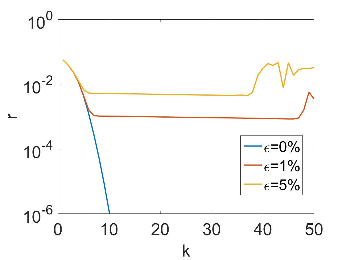
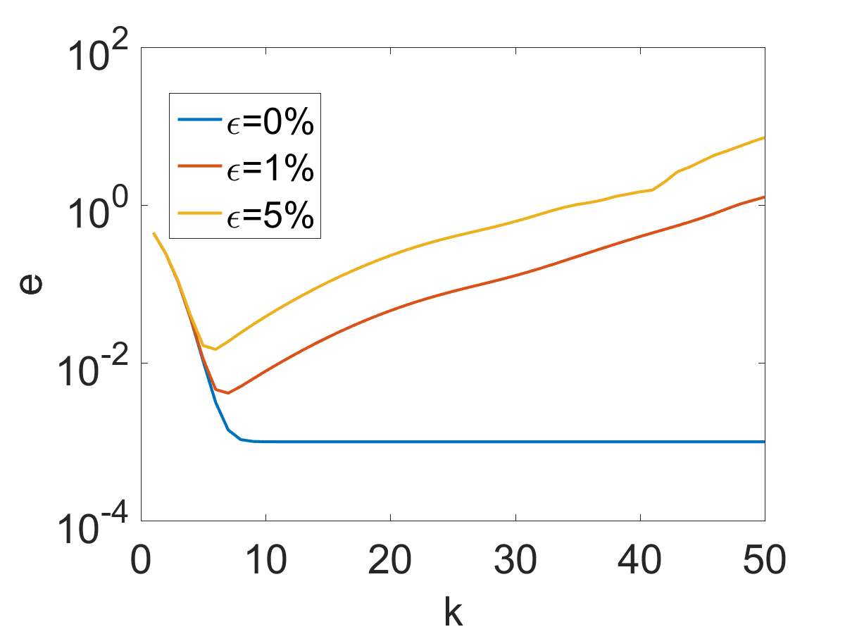
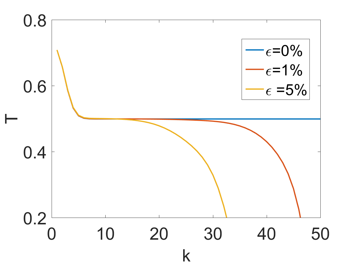
(a) residual $r$	(b) error $e$	(c) terminal time $T$

Figure 1: The convergence of Levenberg-Marquadt method for Example 5.1(i), for $\alpha=0.5$.

Table 1: The numerical results (error $e$, stopping index $k^{*}$ and recovered $\hat{T}$) for Example 5.1. For case (i), $\gamma_{0}=\text{1e-2}$, $\mu_{0}=\text{2.7e-3}$, 6.3e-3 and 1.3e-2 for $\alpha=0.25$, $0.50$ and $0.75$, respectively, and $\rho=0.80$; for case (ii), $\gamma_{0}=\text{1e-3}$, $\mu_{0}=\text{1.1e-4}$, 2.7e-4, and 6e-4 for $\alpha=0.25$, $0.50$ and $0.75$, respectively, and $\rho=0.80$.

case	$\alpha$	$0.25$			$0.50$			$0.75$
	$\epsilon$	$e$	$k^{*}$	$\hat{T}$	$e$	$k^{*}$	$\hat{T}$	$e$	$k^{*}$	$\hat{T}$
	0e-3	1.221e-3	16	0.496	9.948e-4	20	0.498	5.023e-4	31	0.500
	1e-3	1.455e-3	8	0.496	1.210e-3	8	0.499	7.217e-4	10	0.500
(i)	5e-3	2.961e-3	7	0.496	2.468e-3	7	0.499	1.852e-3	9	0.500
	1e-2	4.793e-3	6	0.498	4.114e-3	7	0.499	3.275e-3	9	0.500
	2e-2	8.121e-3	6	0.498	6.872e-3	6	0.501	5.578e-3	8	0.502
	5e-2	1.675e-2	5	0.505	1.476e-2	6	0.502	1.230e-2	8	0.503
	0e-3	7.368e-2	32	0.496	7.414e-2	33	0.500	7.586e-2	36	0.498
	1e-3	7.574e-2	15	0.497	7.622e-2	17	0.500	7.799e-2	20	0.498
(ii)	5e-3	8.230e-2	11	0.497	8.315e-2	13	0.500	8.648e-2	17	0.498
	1e-2	9.119e-2	10	0.497	9.247e-2	11	0.500	9.737e-2	15	0.498
	3e-2	1.169e-1	6	0.497	1.186e-1	7	0.500	1.235e-1	7	0.499
	5e-2	1.281e-1	4	0.499	1.275e-1	4	0.503	1.300e-1	6	0.501

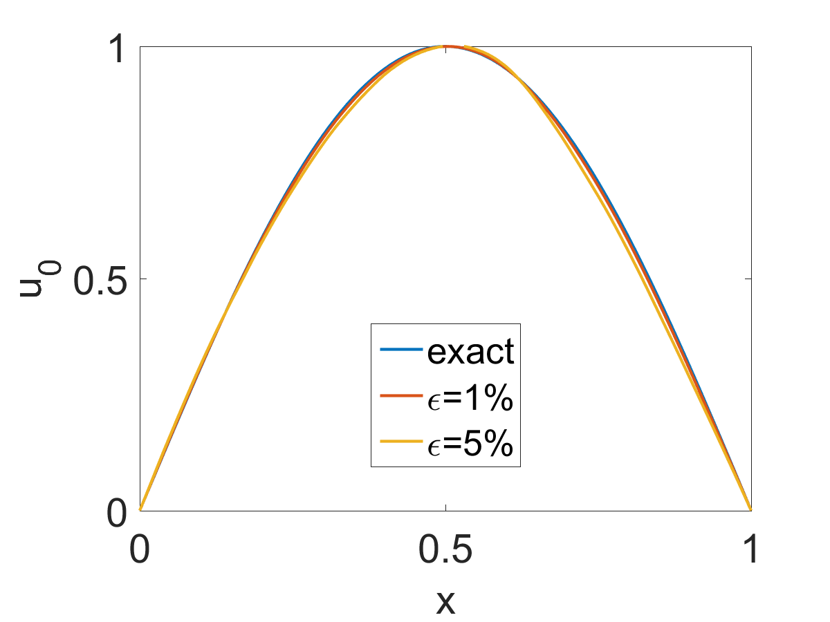
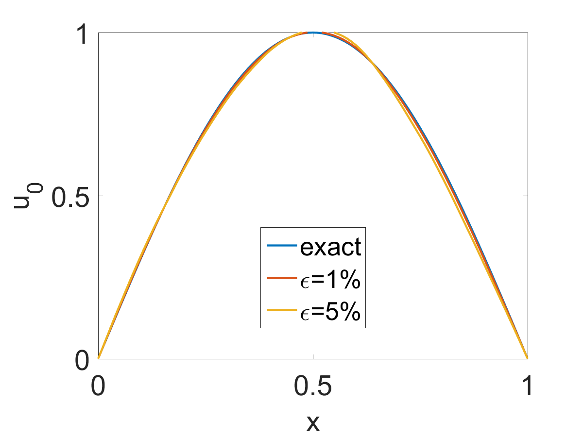
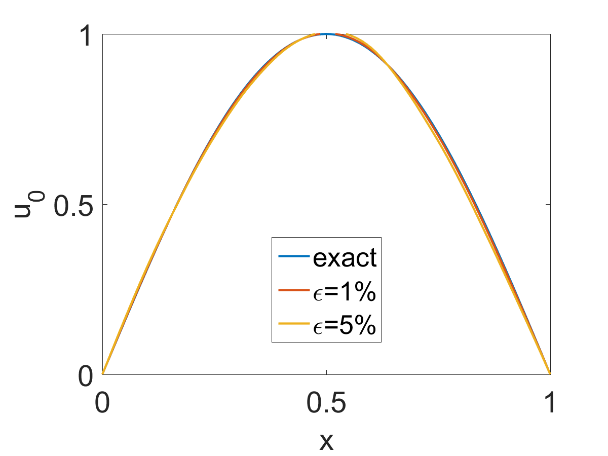
(a) $\alpha=0.25$	(b) $\alpha=0.50$	(c) $\alpha=0.75$

Figure 2: The reconstructions of the initial condition $u_{0}$ for Example 5.1(i).

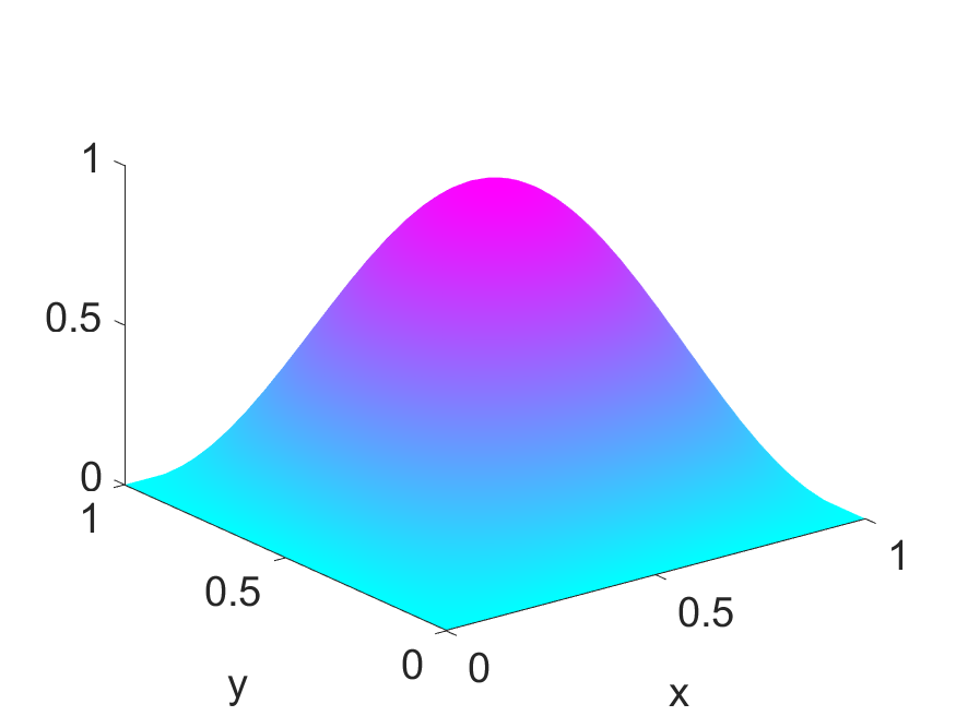
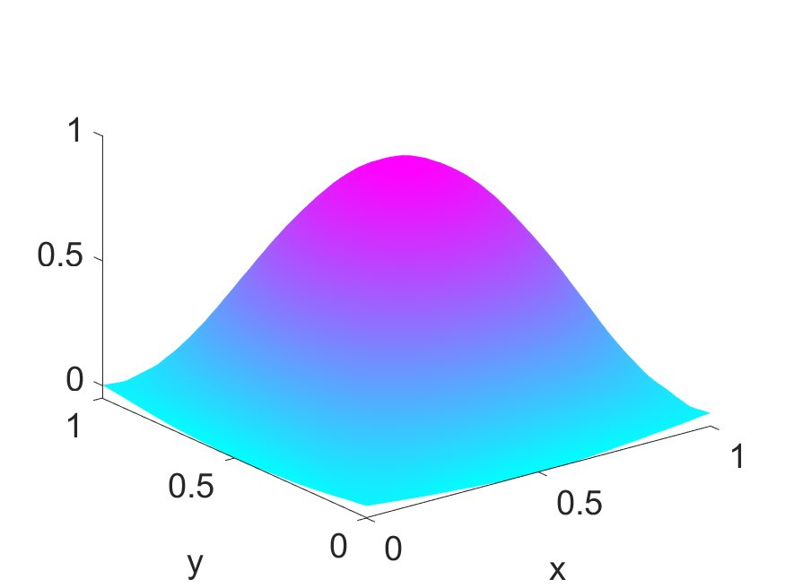
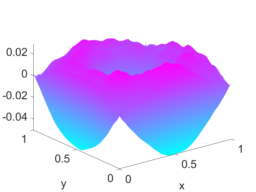
(a) exact	(b) reconstruction	(c) error

Figure 3: The reconstructions of the initial condition $u_{0}$ for Example 5.1(ii) with $\alpha=0.5$, $\epsilon=5\%$.

The next example is about ISP, with $q\equiv 0$.

Example 5.2.

• The initial condition $u_{0}=\sin(2\pi x)$, and the unknown source $\psi(x)=\sin(3\pi x)$.

• The known diffusion coefficient $a=1+\sin(\pi x)y(1-y)$, initial condition $u_{0}=\sin(\pi x)\sin(\pi y)$, and the unknown source $\psi=4x(1-x)e^{x}\sin(2\pi y)$.

The numerical results for Example 5.2 are shown in Figs. 4, 5 and 6, and Table 2. The convergence plots in Fig. 4 show the semiconvergence phenomenon, and with the chosen parameters, the method converges rapidly to an acceptable solution, and then the error $e$ starts to increase shortly afterwards. Nonetheless, the estimate of $T$ converges fairly fast (within 5 iterations), and it is also quite stable during the iteration. We obtain very accurate reconstructions for the noise level $\epsilon$ up to 5e-2. Like before, the reconstruction quality does not depend much on the order $\alpha$, cf. Table 2 and Fig. 5, concurring with the observations for BP. The latter also agrees with the fact that ISP enjoys similar stability as BP, as indicated by Theorems 2.2 and 3.2.

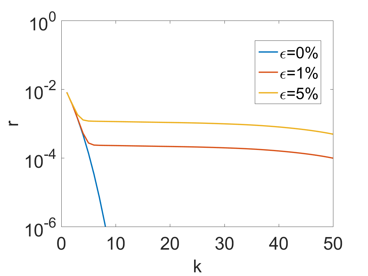
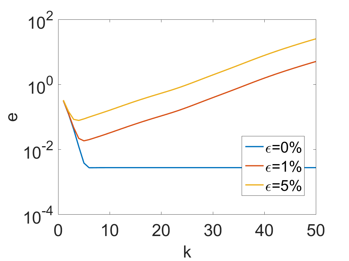
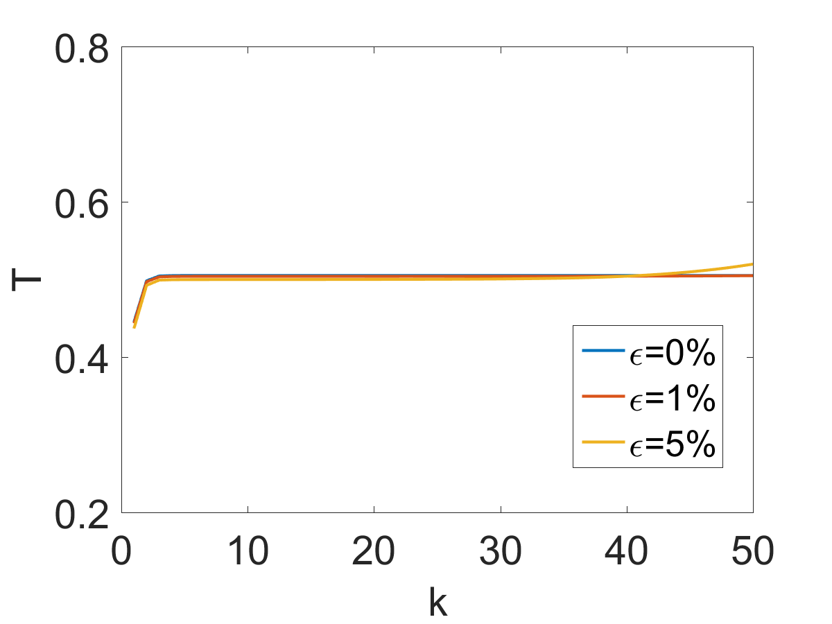
(a) residual $r$	(b) error $e$	(c) terminal time $T$

Figure 4: The convergence of the Levenberg-Marquadt method for Example 5.2(i) with $\alpha=0.5$.

Table 2: The numerical results (error $e$, stopping index $k^{*}$ and recovered $\hat{T}$) for Example 5.2. For case (i), $\gamma_{0}=\text{1e-4}$, $\mu_{0}=\text{1e-8}$, 5e-8 and 1e-7 for $\alpha=0.25,0.50$ and $0.75$, respectively, and $\rho=0.8$; and for case (ii), $\gamma_{0}=\text{1e-4}$, $\mu_{0}=\text{1e-9}$ and $\rho=0.8$.

case	$\alpha$	$0.25$			$0.50$			$0.75$
	$\epsilon$	$e$	$k^{*}$	$\hat{T}$	$e$	$k^{*}$	$\hat{T}$	$e$	$k^{*}$	$\hat{T}$
	0e-3	2.534e-3	6	0.507	2.709e-3	6	0.505	3.057e-3	6	0.506
	1e-3	3.402e-3	6	0.507	3.381e-3	6	0.504	3.417e-3	6	0.506
(i)	5e-3	1.098e-2	5	0.506	1.000e-2	5	0.504	8.016e-3	6	0.505
	1e-2	2.035e-2	5	0.505	1.825e-2	5	0.503	1.410e-2	5	0.505
	2e-2	3.839e-2	4	0.503	3.488e-2	4	0.502	2.669e-2	5	0.504
	5e-2	8.668e-2	4	0.496	7.761e-2	4	0.499	5.944e-2	4	0.501
	0e-3	2.122e-1	35	0.514	2.121e-1	35	0.508	2.119e-1	35	0.509
	1e-3	2.173e-1	9	0.514	2.171e-1	9	0.508	2.166e-1	10	0.509
(ii)	5e-3	2.223e-1	4	0.515	2.218e-1	4	0.509	2.206e-1	5	0.509
	1e-2	2.276e-1	3	0.516	2.267e-1	3	0.509	2.250e-1	3	0.509
	3e-2	2.626e-1	3	0.522	2.576e-1	3	0.512	2.477e-1	3	0.512
	5e-2	2.843e-1	2	0.519	2.797e-1	2	0.507	2.707e-1	2	0.500

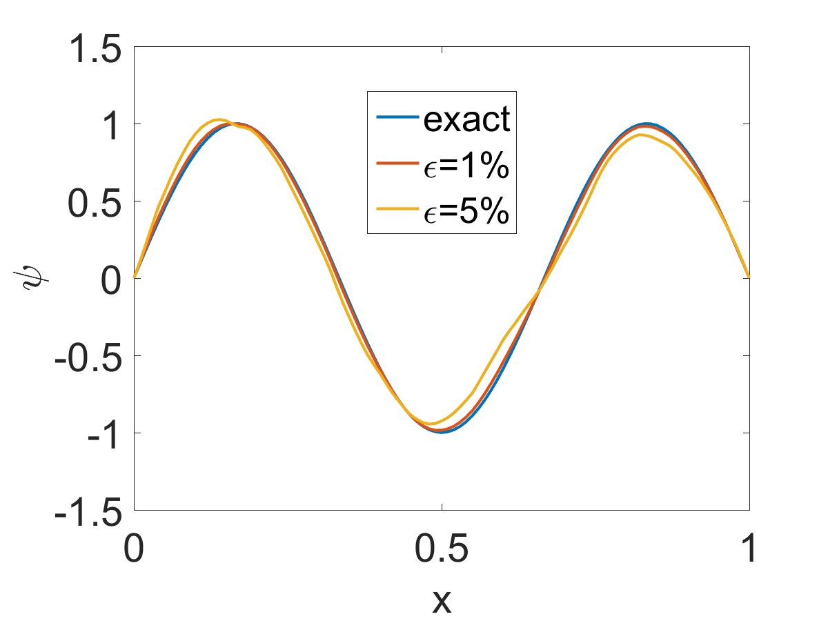
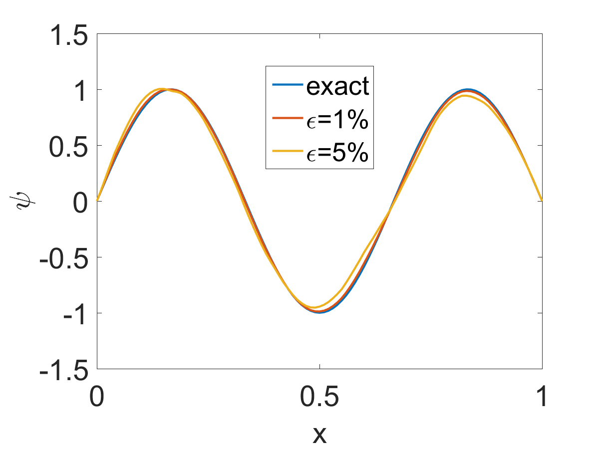
(a) $\alpha=0.25$	(b) $\alpha=0.50$	(c) $\alpha=0.75$

Figure 5: The reconstructions of the space-dependent source $\psi$ for Example 5.2(i).

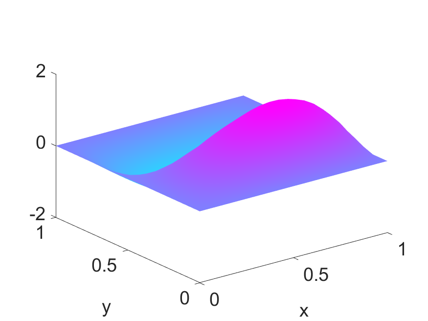
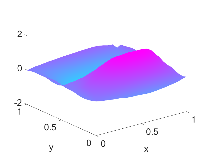
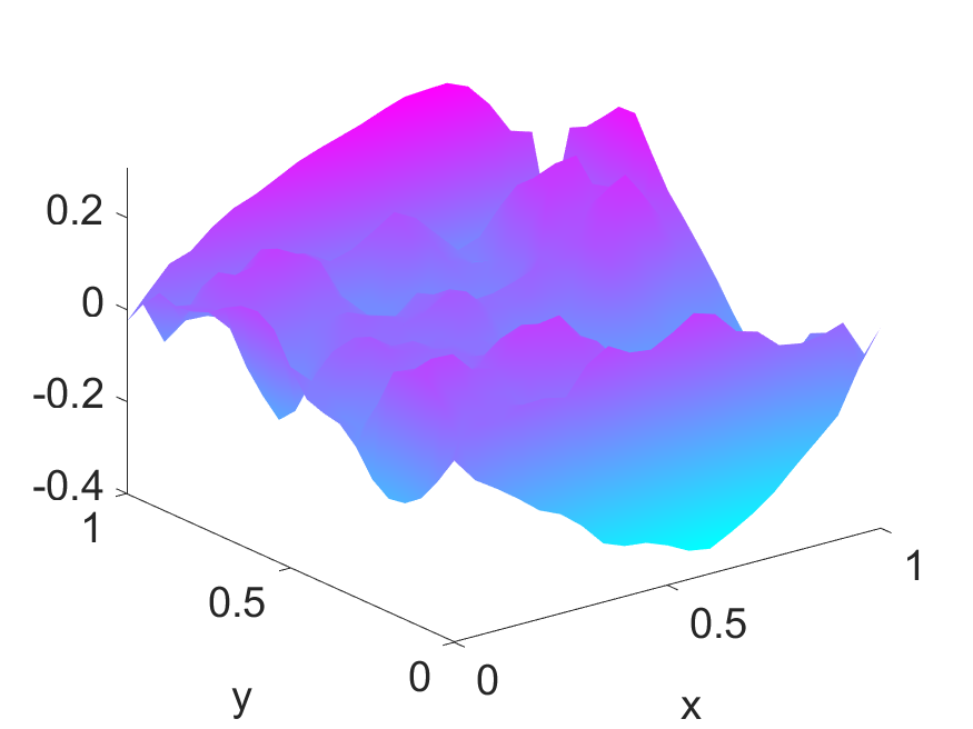
(a) exact	(b) reconstruction	(c) pointwise error

Figure 6: The reconstructions of the space source component $\psi$ for Example 5.2(ii) with $\alpha=0.5$, $\epsilon=5\%$.

The last example is about IPP in 1D.

Example 5.3.

The source $f=|\sin(2\pi x)|$, initial condition $u_{0}\equiv 1$, and a zero Dirichlet boundary condition. The unknown potential $q=\sin^{4}(\pi x)$.

The parameter $\gamma_{0}$ is fixed at 1e-7 and $\mu_{0}$ at 1e-8, and the decreasing factor $\rho$ is set to $0.5$. The numerical results are summarized in Figs. 7 and 8. Note that we can obtain highly accurate reconstructions for exact data, with the $L^{2}(\Omega)$ error of the recovered potential $\hat{q}$ being 1.318e-3, 1.374e-3 and 1.174e-3 for $\alpha=0.25$, 0.50 and 0.75, respectively. The estimated terminal time $T=0.4996$, 0.4997 and 0.4998 for $\alpha=0.25$, 0.50 and 0.75, respectively, are also fairly accurate. This clearly shows the feasibility of simultaneous recovery. However, for noisy data, the recovery is very challenging. Numerically we observe that the singular value spectrum of the linearized forward operator has many tiny values (and hence we have to use a tiny value for the parameter $\gamma_{0}$), which precludes applying any realistic amount of noise to the data and renders the recovery from noisy data highly unstable.

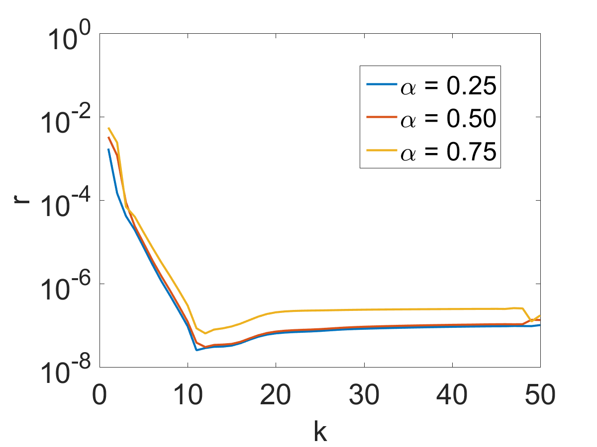
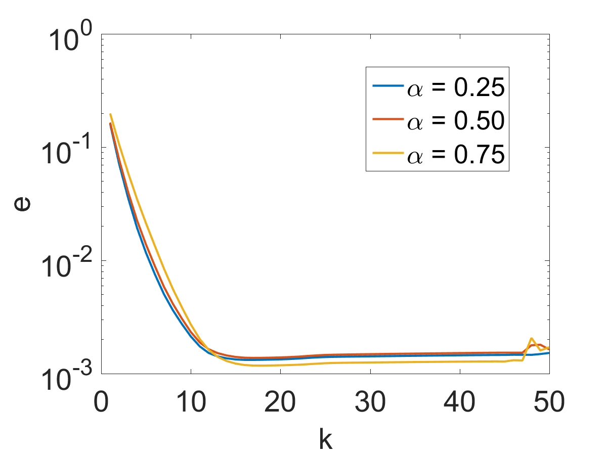
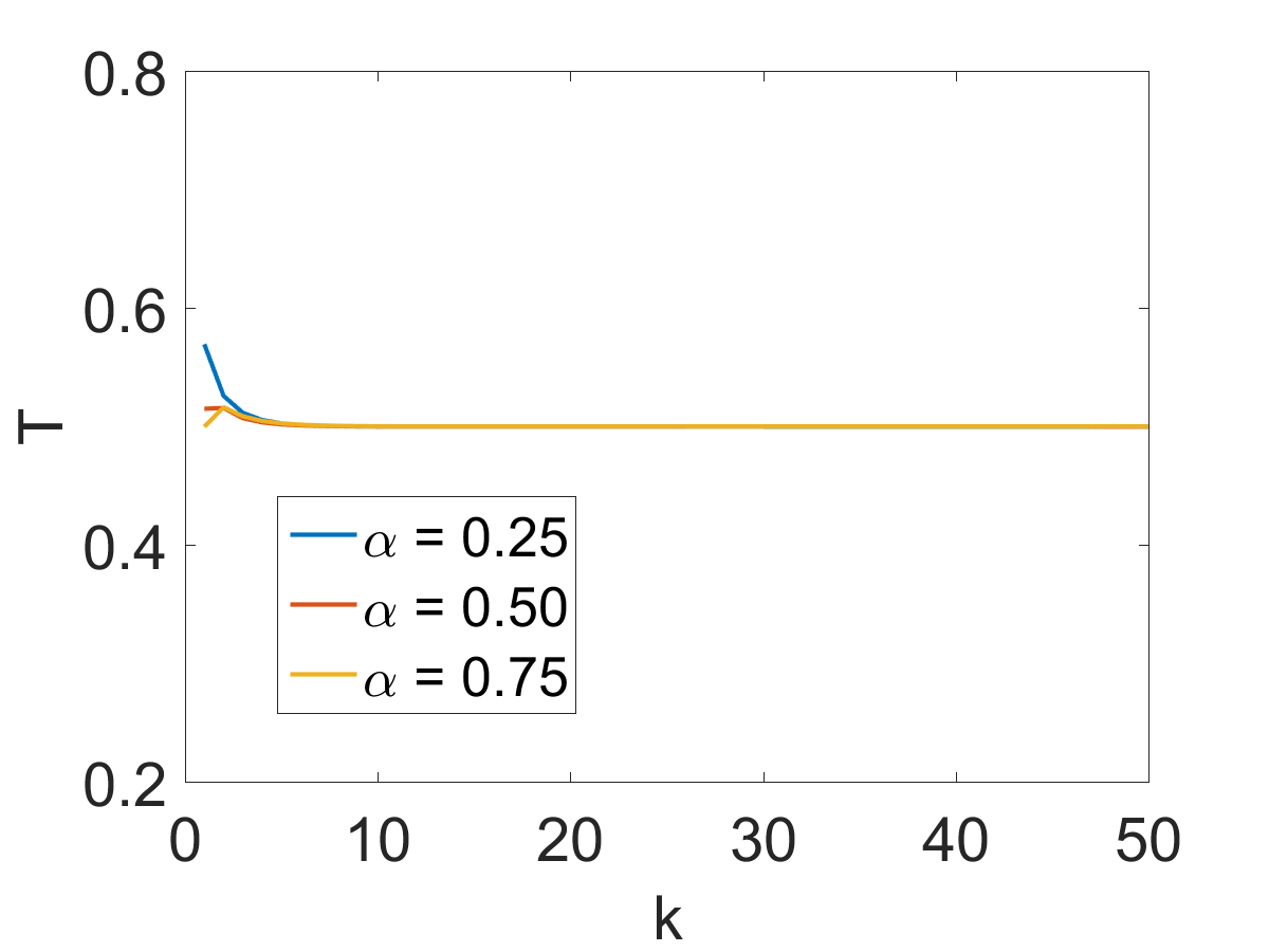
(a) residual $r$	(b) error $e$	(c) terminal time $T$

Figure 7: The convergence of the Levenberg-Marquadt method for Example 5.3 with exact data.

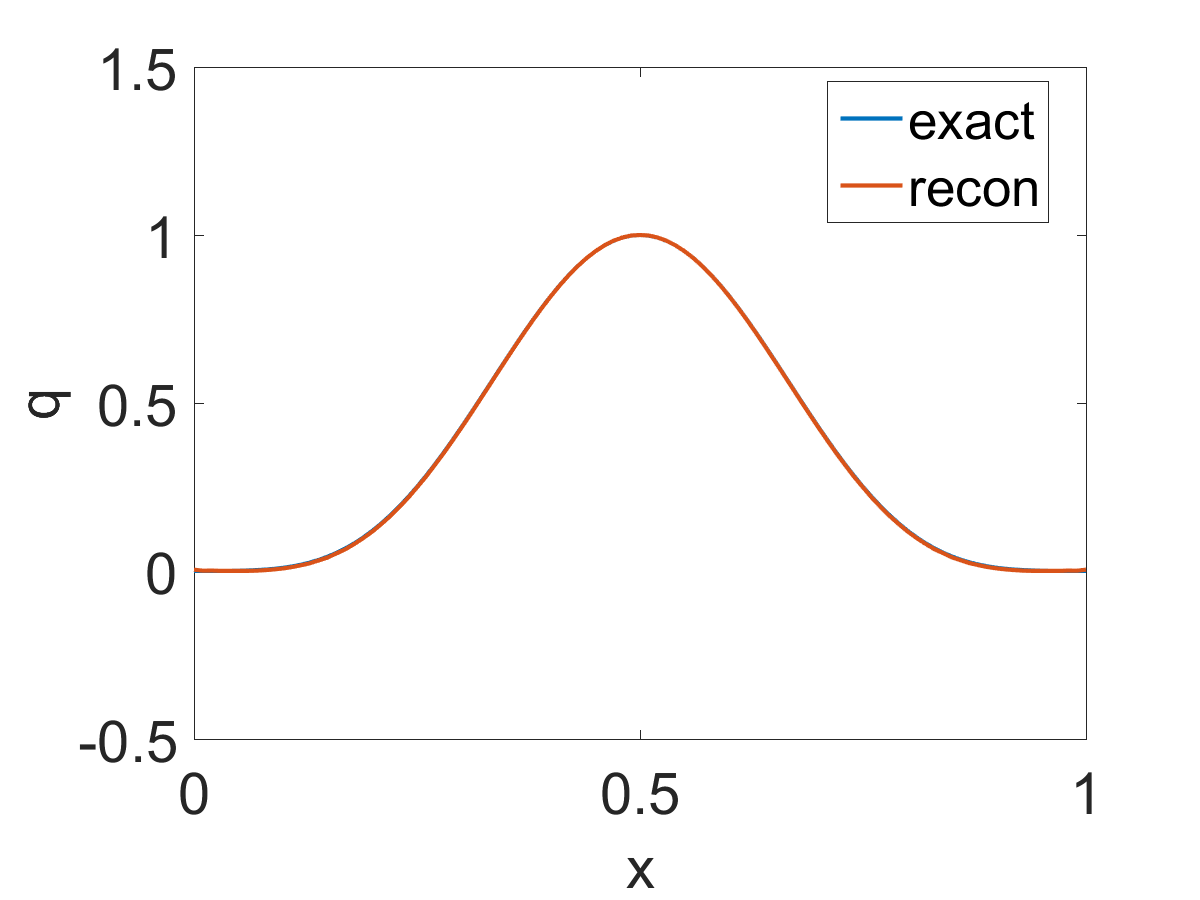
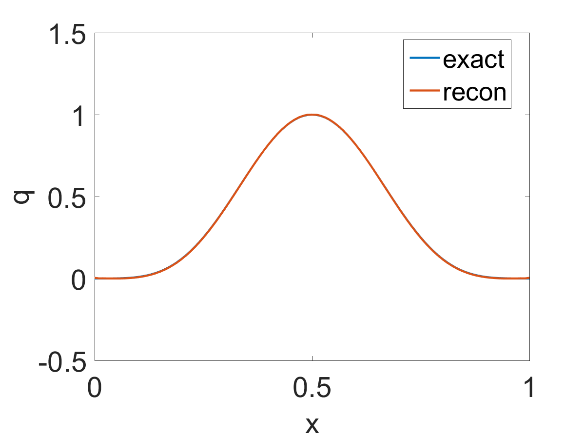
(a) $\alpha=0.25$	(b) $\alpha=0.50$	(c) $\alpha=0.75$

Figure 8: The reconstructions of the space-dependent potential $q$ for Example 5.3 with exact data.

References

- [1] E. E. Adams and L. W. Gelhar. Field study of dispersion in a heterogeneous aquifer: 2. spatial moments analysis. Water Res. Research, 28(12):3293–3307, 1992.
- [2] Y. Hatano and N. Hatano. Dispersive transport of ions in column experiments: An explanation of long-tailed profiles. Water Res. Research, 34(5):1027–1033, 1998.
- [3] J. Janno and N. Kinash. Reconstruction of an order of derivative and a source term in a fractional diffusion equation from final measurements. Inverse Problems, 34(2):025007, 19, 2018.
- [4] B. Jin. Fractional Differential Equations—An Approach via Fractional Dderivatives, volume 206 of Applied Mathematical Sciences. Springer, Cham, 2021.
- [5] B. Jin, R. Lazarov, and Z. Zhou. Error estimates for a semidiscrete finite element method for fractional order parabolic equations. SIAM J. Numer. Anal., 51(1):445–466, 2013.
- [6] B. Jin, R. Lazarov, and Z. Zhou. An analysis of the L1 scheme for the subdiffusion equation with nonsmooth data. IMA J. Numer. Anal., 36(1):197–221, 2016.
- [7] B. Jin and W. Rundell. A tutorial on inverse problems for anomalous diffusion processes. Inverse Problems, 31(3):035003, 40, 2015.
- [8] B. Jin and Z. Zhou. An inverse potential problem for subdiffusion: stability and reconstruction. Inverse Problems, 37(1):Paper No. 015006, 26, 2021.
- [9] B. Kaltenbacher and W. Rundell. On an inverse potential problem for a fractional reaction-diffusion equation. Inverse Problems, 35(6):065004, 31, 2019.
- [10] A. A. Kilbas, H. M. Srivastava, and J. J. Trujillo. Theory and Applications of Fractional Differential Equations. Elsevier Science B.V., Amsterdam, 2006.
- [11] S. C. Kou. Stochastic modeling in nanoscale biophysics: subdiffusion within proteins. Ann. Appl. Stat., 2(2):501–535, 2008.
- [12] A. Kubica, K. Ryszewska, and M. Yamamoto. Time-Fractional Differential Equations. Springer, Singapore, 2020. A theoretical introduction.
- [13] K. Levenberg. A method for the solution of certain non-linear problems in least squares. Quart. Appl. Math., 2:164–168, 1944.
- [14] B. M. Levitan and I. S. Sargsjan. Introduction to Spectral Theory: Selfadjoint Ordinary Differential Operators. American Mathematical Society, Providence, R.I., 1975.
- [15] Z. Li and M. Yamamoto. Inverse problems of determining coefficients of the fractional partial differential equations. In Handbook of fractional calculus with applications. Vol. 2, pages 443–464. De Gruyter, Berlin, 2019.
- [16] K. Liao and T. Wei. Identifying a fractional order and a space source term in a time-fractional diffusion-wave equation simultaneously. Inverse Problems, 35(11):115002, 23, 2019.
- [17] Y. Liu, Z. Li, and M. Yamamoto. Inverse problems of determining sources of the fractional partial differential equations. In Handbook of Fractional Calculus with Applications. Vol. 2, pages 411–429. De Gruyter, Berlin, 2019.
- [18] Y. Luchko and M. Yamamoto. On the maximum principle for a time-fractional diffusion equation. Fract. Calc. Appl. Anal., 20(5):1131–1145, 2017.
- [19] D. W. Marquardt. An algorithm for least-squares estimation of nonlinear parameters. J. Soc. Indust. Appl. Math., 11:431–441, 1963.
- [20] K. S. Miller and S. G. Samko. A note on the complete monotonicity of the generalized Mittag-Leffler function. Real Anal. Exchange, 23(2):753–755, 1997/98.
- [21] R. R. Nigmatulin. The realization of the generalized transfer equation in a medium with fractal geometry. Phys. Stat. Sol. B, 133:425–430, 1986.
- [22] K. Sakamoto and M. Yamamoto. Initial value/boundary value problems for fractional diffusion-wave equations and applications to some inverse problems. J. Math. Anal. Appl., 382(1):426–447, 2011.
- [23] W. R. Schneider. Completely monotone generalized Mittag-Leffler functions. Exposition. Math., 14(1):3–16, 1996.
- [24] T. Simon. Comparing Fréchet and positive stable laws. Electron. J. Probab., 19:no. 16, 25, 2014.
- [25] V. Thomée. Galerkin Finite Element Methods for Parabolic Problems. Springer-Verlag, Berlin, second edition, 2006.
- [26] Z. Zhang, Z. Zhang, and Z. Zhou. Identification of potential in diffusion equations from terminal observation: analysis and discrete approximation. SIAM J. Numer. Anal., 60(5):2834–2865, 2022.
- [27] Z. Zhang and Z. Zhou. Recovering the potential term in a fractional diffusion equation. IMA J. Appl. Math., 82(3):579–600, 2017.
- [28] Z. Zhang and Z. Zhou. Numerical analysis of backward subdiffusion problems. Inverse Problems, 36(10):105006, 27, 2020.