Theory of Energy Dispersion of Chiral Phonons

Abstract

We have developed a microscopic theory on phonon energy dispersion in chiral crystals within a harmonic approximation. One of the main issues is about the splitting of sound velocity of acoustic phonons with opposite “crystal” angular momenta. We have shown that the splitting must be zero even in chiral crystals and the difference starts from the order of at least $k^{2}$ or higher in their energy dispersion. Splitting is evident for chiral optical phonons, and we have derived a formula for their $k$-linear splitting. Another important finding is about possible interactions of atomic displacements in microscopic models. We have found that antisymmetric interactions of $\bm{D}_{ij}\cdot(\bm{d}_{i}\times\bm{d}_{j})$ type are not allowed in microscopic Hamiltonians for chiral phonons because of the stability of equilibrium structure. We have identified that the splitting in both acoustic and optical modes arises from the harmonic potentials with the electric toroidal quadrupole of $G_{u}$-type symmetry. These constraint are important for modeling real materials. Most of our microscopic calculations have been performed for (quasi-)one-dimensional systems with a trigonal crystal symmetry including Te, but these results generally hold also for other chiral phonon systems.

Chirality is a three-dimensional geometric concept that is defined by the absence of any mirror and inversion operations in systems under consideration[1, 2]. Dynamical aspects of chirality in materials and fields have been also emphasized by Barron[3], and the microscopic definition of chirality has been recently introduced in terms of electronic multipoles[4, 5]. Since the proper rotation operations (and translations in crystals) alone cannot distinguish the difference between polar and axial properties, it allows systems to have a variety of couplings among axial and polar quantities such as electric field and angular momentum. It leads to chirality specific cross-correlated responses discussed in many research fields such as biochemistry[6], nano-optics[7, 8], nonmagnetic inorganic crystals[9, 10, 11, 12, 4], and magnetism[13, 14, 15, 16]. Furthermore, the spin degrees of freedom even in nonmagnetic materials are also involved in the so-called “Chirality-Induced Spin Selectivity” (CISS), which has been actively studied [17, 18, 19, 20, 21, 22, 23, 24].

In particular, phonons in chiral crystals[25, 26, 27, 28, 29, 30, 31, 32] have attracted much interest because their transverse modes are characterized by the quantum numbers of proper “crystal” angular momentum (CAM) about the chiral axis [33, 34, 35, 36, 37, 38]. The CAM related phenomena have been widely reported such as spin relaxation[39, 40, 41], phonon-magnon conversion[42, 43], orbital magnetization due to phonons[44], phonon induced current[45], and correction to the Einstein-de Haas effect[34]. The selection rule of CAM has been examined by the Raman scattering experiment[46]. Its relation to CISS has been also investigated as a source of spin filtering[47]. Moreover, superconductivity has been observed in chiral crystals, Li₂Pd₃B and Li₂Pt₃B[48, 49, 50], and its pairing mechanism due to electron-phonon coupling is elucidated[49].

In the theoretical aspect on the chiral phonons, the symmetry argument of the dielectric tensor[51], and the effective continuum field theory including rigid-body rotations[52] based on the micropolar elastic theory[53, 54] have been developed. The energy dispersions[25, 26], acoustic activity in the $\alpha$ quartz[27] and the roton-like excitation in metamaterials[55] have been indeed observed. On the other hand, the origin of characteristics of chiral phonons remains obscure, despite extensive studies based on microscopic models or first-principle calculations[27, 28, 29, 30, 32, 37]. For example, what type of harmonic interactions cause the energy splitting of chiral phonons with opposite CAM remains unknown. In particular, as the splitting of acoustic phonons has a close relation to the stability of the given lattice structure, concrete constraint for chiral phonons is crucial for modeling real materials on the basis of the first-principle calculations. Indeed, it is known that the first principles phonon calculations sometimes become unstable in chiral crystals[56, 57, 58].

In this letter, we have developed a microscopic theory on phonon energy dispersion in chiral crystals within a harmonic approximation, and elucidated some rigorous constraints and a source of splitting for opposite CAM modes. One of the textbook examples of chiral crystals is Te[59] and its phonon properties have also been studied both experimentally and theoretically[26, 27, 28, 29, 30, 32]. So, let us first pick up this system and identify phonon properties characteristic to its chiral crystal structure.

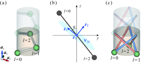
Figure 1: (Color online) (a) A single helix in a Te-like lattice. (b) Stiffness matrix $\mathsf{v}_{2,0}$ and its principle axes $\{\tilde{\bm{e}}_{j}\}$. (c) A double-handed triple helix. Left and right bonds are colored in blue and red, respectively.

At ambient pressure, Te has a crystal structure categorized to the space group $P3_{1}21$ (No. 152) corresponding to the trigonal chiral point group $D_{3}$. Its mirror image belongs to $P3_{2}21$ (No. 154) This structure is a hexagonal lattice made of helices running along the $z$-direction, and the unit cell contains three sublattice sites as shown in Fig. 1(a). While the primitive lattice vector $\bm{a}_{3}\mspace{-3.0mu}=\mspace{-3.0mu}c(0,0,1)$ is along the $c$-axis, $\bm{a}_{1}\mspace{-3.0mu}=\mspace{-3.0mu}a(1,0,0)$ and $\bm{a}_{2}\mspace{-3.0mu}=\mspace{-3.0mu}a(-\frac{1}{2},\frac{\sqrt{3}}{2},0)$ span the $ab$-plane, and we also define the supplementary vector $\bm{a}_{0}\mspace{-3.0mu}=\mspace{-3.0mu}-\bm{a}_{1}\mspace{-2.0mu}-\mspace{-2.0mu}\bm{a}_{2}$. The site position of the three sublattices is then represented as

$$\bm{r}_{l}=\bm{s}_{l}+\bm{r},\ \ \bm{s}_{l}=\delta\,\bm{a}_{l}+{\textstyle\frac{1}{3}}l\,\bm{a}_{3},\ \ (l=0,1,2),$$ (1)

where $\bm{r}\mspace{-3.0mu}=\mspace{-3.0mu}\sum_{j=1}^{3}n_{j}\bm{a}_{j}$ with integer $n_{j}$’s is the unit cell position. For Te, the value of $\delta$ is about 0.23[60], but we let it be a free parameter $0\mspace{-2.0mu}<\mspace{-2.0mu}\delta\mspace{-2.0mu}<\mspace{-2.0mu}\frac{1}{2}$ and consider more general cases. Site connectivity in each helix is described by the nearest-neighbor bonds $\bm{t}_{l,l+1}\mspace{-2.0mu}\equiv\mspace{-2.0mu}\bm{s}_{l+1}\mspace{-2.0mu}-\mspace{-2.0mu}\bm{s}_{l}\mspace{-2.0mu}+\mspace{-2.0mu}\delta_{l,2}\mspace{2.0mu}\bm{a}_{3}$ each connecting $l$ and $l\mspace{-2.0mu}+\mspace{-2.0mu}1$ sublattices. One should understand as $l\mspace{-2.0mu}+\mspace{-2.0mu}1\mspace{-3.0mu}=\mspace{-3.0mu}3\mspace{-2.0mu}\equiv\mspace{-2.0mu}0$ as well as $l\mspace{-2.0mu}-\mspace{-2.0mu}1\mspace{-3.0mu}=\mspace{-3.0mu}-1\mspace{-2.0mu}\equiv\mspace{-2.0mu}2$ for the sublattice index throughout this paper.

Now we summarize the procedure of calculating phonon energy dispersion. A starting point is a lattice deformation energy functional $\mathscr{V}$ represented in terms of atomic displacements $\{\bm{d}(\bm{r}_{l})\}$, and it is customary for it to employ a quadratic form of $\{\bm{d}(\bm{r}_{l})\}$. After Fourier transformation, the coefficient in the quadratic form for each wavevector $\bm{k}$ is reduced to a matrix with the dimension of $3\mspace{-1.0mu}\times\mspace{-1.0mu}\mbox{(no.~{}of sublattices)}$. This is called the dynamical matrix, and its each eigenvalue $\lambda_{\alpha\bm{k}}$ determines the corresponding phonon energy dispersion as $\hbar\omega_{\alpha\bm{k}}\mspace{-3.0mu}=\mspace{-3.0mu}\hbar\sqrt{\lambda_{\alpha\bm{k}}/M}$ with the atomic mass $M$. Since our concern is their $\bm{k}$-dependence, we use the units of $M\mspace{-3.0mu}=\mspace{-3.0mu}1$ and $\hbar\mspace{-3.0mu}=\mspace{-3.0mu}1$. In this paper, we treat for simplicity the cases that constituent atoms are all identical and they have an isotropic mass tensor, but it is straightforward to generalize these points.

Let us then construct a simple model for the deformation energy $\mathscr{V}$ describing two-atom interactions as explained before. To this end, two requirements are crucial. First, its energy must be non-negative for any displacements to guarantee the stability of the equilibrium structure. Secondly, its functional form must match the lattice symmetry. Namely, it should be invariant upon any symmetry operation of the lattice. Considering $\mathscr{V}$ is scalar, a product of two displacement vectors $\bm{d}\mspace{-3.0mu}=\mspace{-3.0mu}\bm{d}(\bm{r}_{l})$ and $\bm{d}^{\prime}\mspace{-3.0mu}=\mspace{-3.0mu}\bm{d}(\bm{r}_{m})$ appears in it with a coefficient that is either a scalar ($v$), symmetric second-rank tensor ($v_{i\mspace{-1.0mu}j}\mspace{-3.0mu}=\mspace{-3.0mu}v_{j\mspace{1.0mu}i}$), or antisymmetric tensor ($v_{ij}\mspace{-3.0mu}=\mspace{-3.0mu}\epsilon_{i\mspace{-1.0mu}j\mspace{1.0mu}k}D_{k}$). The last case corresponds to an interaction of Dzyloshinskii-Moriya (DM) type $\bm{D}\cdot(\bm{d}\times\bm{d}^{\prime})$, but this type is not allowed in our case. Clearly, it does not fulfill the first requirement, and one cannot resolve this problem by generalizing its form. The remaining two cases are all together summarized to a quadratic form $(\bm{d}\mspace{-2.0mu}-\mspace{-2.0mu}\bm{d}^{\prime})\cdot\mathsf{v}\,(\bm{d}\mspace{-2.0mu}-\mspace{-2.0mu}\bm{d}^{\prime})$ with a real symmetric $3\mspace{-1.0mu}\times\mspace{-1.0mu}3$ matrix $\mathsf{v}\mspace{-3.0mu}=\mspace{-3.0mu}\mathsf{v}(\bm{r}_{l}\mspace{-2.0mu}-\mspace{-2.0mu}\bm{r}_{m})$, which will be referred to as stiffness matrix henceforth. This complies with the first requirement, if $\mathsf{v}$ has no negative eigenvalue. Furthermore, energy cost is zero when $\bm{d}\mspace{-3.0mu}=\mspace{-3.0mu}\bm{d}^{\prime}$, which meets our expectation for $\mathscr{V}$ since the related atomic bond is intact. The second requirement imposes that $\mathsf{v}$’s principal axes $\{\tilde{\bm{e}}_{i}\}$ ($i\mspace{-3.0mu}=\mspace{-3.0mu}1,2,3$) point to the local symmetric directions of the bond connecting the atomic sites $\bm{r}_{l}$ and $\bm{r}_{m}$.

We are ready to write down an explicit form of $\mathscr{V}$ for the case of Te-like lattice with “left” handedness. It consists of a part for inside each helix ($\mathscr{V}_{L,1}$) and a part between neighboring helices ($\mathscr{V}_{L,2}$). The latter part will be discussed later. For $\mathscr{V}_{L,1}$, we consider contributions of only nearest-neighbor pairs

$$\mathscr{V}_{L,1}=\!\sum_{\bm{r}_{l}}\bigl{[}\bm{d}(\bm{r}_{l})\mspace{-2.0mu}-\mspace{-2.0mu}\bm{d}(\bm{r}_{l}\mspace{-2.0mu}+\mspace{-2.0mu}\bm{t}_{l,l+1})\bigr{]}\cdot\mathsf{v}_{l,l+1}\,\bigl{[}\bm{d}(\bm{r}_{l})\mspace{-2.0mu}-\mspace{-2.0mu}\bm{d}(\bm{r}_{l}\mspace{-2.0mu}+\mspace{-2.0mu}\bm{t}_{l,l+1})\bigr{]},$$ (2)

where $\mathsf{v}_{l,l+1}$ is the stiffness matrix for the bond $\bm{t}_{l,l+1}$ and is subject to the symmetry constraints $\mathsf{v}_{2,0}\mspace{-3.0mu}=\mspace{-3.0mu}\mathsf{C}_{3}\mathsf{v}_{0,1}\mathsf{C}_{3}^{T}\mspace{-3.0mu}=\mspace{-3.0mu}\mathsf{C}_{3}^{T}\mathsf{v}_{1,2}\mathsf{C}_{3}$. Here, $\mathsf{C}_{3}$ is the $3\mspace{-1.0mu}\times\mspace{-1.0mu}3$ matrix of clockwise rotation by the angle ${\textstyle\frac{2\pi}{3}}$ about the $z$-axis, and the symbol $T$ denotes a matrix transposition. As for the bond $\bm{t}_{2,0}$, it remains intact under the $\pi$-rotation about the $x$-axis $C_{2x}^{\prime}$, and therefore one principle axis needs to be $\tilde{\bm{e}}_{1}\mspace{-3.0mu}=\mspace{-3.0mu}(1,0,0)^{T}$. This leads to a parametrization for the other axes as $\tilde{\bm{e}}_{3}\mspace{-3.0mu}=\mspace{-3.0mu}(0,-s_{\theta},c_{\theta})^{T}$ and $\tilde{\bm{e}}_{2}\mspace{-3.0mu}=\mspace{-3.0mu}(0,c_{\theta},s_{\theta})^{T}$ with short hand notations $s_{\theta}\mspace{-3.0mu}=\mspace{-3.0mu}\sin\theta$ and $c_{\theta}\mspace{-3.0mu}=\mspace{-3.0mu}\cos\theta$, but the lattice symmetry provides no further constraints to the $\theta$ value (see Fig. 1(b)). Nonetheless, it is reasonable to expect that one local axis is close to the bond direction $\tilde{\bm{e}}_{3}\mspace{-2.0mu}\sim\mspace{-2.0mu}\bm{t}_{2,0}/|\bm{t}_{2,0}|$. If they coincide, the value is then $\theta\mspace{-3.0mu}=\mspace{-3.0mu}\tan^{-1}(\!\sqrt{27}\mspace{2.0mu}\delta\mspace{2.0mu}a/c)$. For the $\bm{t}_{2,0}$ bond, using its local axes $\tilde{\bm{e}}_{i}$’s discussed above, we can write down its stiffness matrix as

$$\mathsf{v}_{2,0}=\sum_{i=1}^{3}K_{i}\,\tilde{\bm{e}}_{i}\,\tilde{\bm{e}}_{i}^{T}=\left[\begin{array}[]{@{}c@{\hs{1mm}}c@{\hs{1mm}}c@{}}K_{11}\hfil\hskip 2.84526pt&0\hfil\hskip 2.84526pt&0\\ 0\hfil\hskip 2.84526pt&\phantom{-}K_{22}\hfil\hskip 2.84526pt&-\varDelta K\\ 0\hfil\hskip 2.84526pt&-\varDelta K\hfil\hskip 2.84526pt&\phantom{-}K_{33}\end{array}\right]=:\bar{\mathsf{v}},\vspace{-4pt}$$ (3)

where $K_{i}$’s are non-negative stiffness constants, and $K_{11}\mspace{-3.0mu}=\mspace{-3.0mu}K_{1}$, $K_{22}\mspace{-3.0mu}=\mspace{-3.0mu}K_{2}c_{\theta}^{2}\mspace{-2.0mu}+\mspace{-2.0mu}K_{3}s_{\theta}^{2}$, $K_{33}\mspace{-3.0mu}=\mspace{-3.0mu}K_{2}s_{\theta}^{2}\mspace{-2.0mu}+\mspace{-2.0mu}K_{3}c_{\theta}^{2}$, and $\varDelta K\mspace{-3.0mu}=\mspace{-3.0mu}(K_{3}\mspace{-2.0mu}-\mspace{-2.0mu}K_{2})s_{\theta}\mspace{2.0mu}c_{\theta}$. The other stiffness matrices $\mathsf{v}_{0,1}$ and $\mathsf{v}_{1,2}$ can be calculated by multiplying $\mathsf{C}_{3}$ and $\mathsf{C}_{3}^{T}$ to this $\mathsf{v}_{2,0}$.

The next step is Fourier transformation and we obtain the dynamical matrix. We define a 9-dimensional super-vector by combining the displacement vectors in the wavevector $\bm{k}$-space for the three sublattices $\vec{d}(\bm{k})\mspace{-2.0mu}\equiv\mspace{-2.0mu}(\bm{d}_{0}(\bm{k}),\,\bm{d}_{1}(\bm{k}),\,\bm{d}_{2}(\bm{k}))^{T}$. The intra-helix energy then reads as $\mathscr{V}_{L,1}\mspace{-3.0mu}=\mspace{-3.0mu}\sum_{\bm{k}}\vec{d}(-\bm{k})\cdot\underline{V}_{L,1}(\bm{k})\vec{d}(\bm{k})$, and its coefficient $\underline{V}_{L,1}(\bm{k})$ is the dynamical matrix. It is a $9\mspace{-1.0mu}\times\mspace{-1.0mu}9$ hermitian matrix and

$$\underline{V}_{L,1}(\bm{k})\mspace{-2.0mu}=\mspace{-2.0mu}\left[\begin{array}[]{@{}c@{\hs{1mm}}c@{\hs{1mm}}c@{}}\mathsf{C}_{3}^{T}\mspace{1.0mu}\bar{\mathsf{v}}\mspace{2.0mu}\mathsf{C}_{3}\mspace{-2.0mu}+\mspace{-2.0mu}\bar{\mathsf{v}}\hfil\hskip 2.84526pt&-\mathsf{C}_{3}^{T}\mspace{1.0mu}\bar{\mathsf{v}}\mspace{2.0mu}\mathsf{C}_{3}\gamma_{0,1}\hfil\hskip 2.84526pt&-\bar{\mathsf{v}}\gamma_{2,0}^{*}\\[4.0pt] -\mathsf{C}_{3}^{T}\mspace{1.0mu}\bar{\mathsf{v}}\mspace{2.0mu}\mathsf{C}_{3}\gamma_{0,1}^{*}\hfil\hskip 2.84526pt&\mathsf{C}_{3}\mspace{1.0mu}\bar{\mathsf{v}}\mspace{2.0mu}\mathsf{C}_{3}^{T}\mspace{-2.0mu}+\mspace{-2.0mu}\mathsf{C}_{3}^{T}\mspace{1.0mu}\bar{\mathsf{v}}\mspace{2.0mu}\mathsf{C}_{3}\hfil\hskip 2.84526pt&-\mathsf{C}_{3}\mspace{1.0mu}\bar{\mathsf{v}}\mspace{2.0mu}\mathsf{C}_{3}^{T}\gamma_{1,2}\\[4.0pt] -\bar{\mathsf{v}}\gamma_{2,0}\hfil\hskip 2.84526pt&-\mathsf{C}_{3}\mspace{2.0mu}\bar{\mathsf{v}}\mspace{2.0mu}\mathsf{C}_{3}^{T}\gamma_{1,2}^{*}\hfil\hskip 2.84526pt&\bar{\mathsf{v}}\mspace{-2.0mu}+\mspace{-2.0mu}\mathsf{C}_{3}\mspace{2.0mu}\bar{\mathsf{v}}\mspace{2.0mu}\mathsf{C}_{3}^{T}\end{array}\right],$$ (4)

where the phase factors $\gamma_{l,l+1}\mspace{-2.0mu}\equiv\mspace{-2.0mu}\exp(i\bm{k}\mspace{-2.0mu}\cdot\mspace{-2.0mu}\bm{t}_{l,l+1})$ depend on $\bm{k}$.

In the following we consider the case of $\bm{k}\mspace{-3.0mu}=\mspace{-3.0mu}(0,0,k_{z})$ parallel to the screw axis and denote the wavevector dependence by $k_{z}$ alone. In this case, concerning the interaction energy between neighboring helices $\mathscr{V}_{L,2}$, its dominant terms simply renormalize the parameters in $\bar{\mathsf{v}}$ in Eq. (4). Therefore, it suffice to analyze $\underline{V}_{L,1}(k_{z})$ with $\bar{\mathsf{v}}$ which should be understood as a renormalized coupling. Details will be published elsewhere. Then, the three phase factors coincide as $\gamma_{l,l+1}\mspace{-3.0mu}=\mspace{-3.0mu}e^{ip}$ with $p\mspace{-3.0mu}=\mspace{-3.0mu}{\textstyle\frac{1}{3}}k_{z}c$, and $\underline{V}_{L,1}(k_{z})$ has a special symmetry. There exists an orthogonal matrix $\underline{C}_{3}$ that commutes with $\underline{V}_{L,1}(k_{z})$. It is defined by the transformation of the sublattice displacements as $\underline{C}_{3}:{\bm{d}_{l}}(k_{z})\mspace{-3.0mu}=\mspace{-3.0mu}\mathsf{C}_{3}\bm{d}_{l+1}(k_{z})$ for all $l$’s. Since this satisfies the relation $\underline{C}_{3}^{3}\mspace{-3.0mu}=\mspace{-3.0mu}\underline{1}$, its eigenvalues are $\zeta^{m}$ ($m=0,\pm 1$) with $\zeta\mspace{-3.0mu}=\mspace{-3.0mu}e^{\mspace{2.0mu}i2\pi/3}$, and the eigenspaces of $\underline{V}_{L,1}(k_{z})$ are split into the three subspaces each with a different $m$ value. This $m$ is precisely the quantum number of CAM mentioned in the introduction. For later use, we introduce a hermitian operator that determines the value of CAM: $\underline{L}_{z}\equiv(\underline{C}_{3}\mspace{-2.0mu}-\mspace{-2.0mu}\underline{C}_{3}^{\mspace{2.0mu}T})/(\sqrt{3}\mspace{2.0mu}i)$. It is easy to check that its eigenvalues are $m=0$ and $\pm 1$.

Our task is thus reduced to diagonalizing an effective dynamical matrix in each CAM subspace. It is a $3\mspace{-1.0mu}\times\mspace{-1.0mu}3$ hermitian matrix given as

$$\mathsf{v}_{\mathrm{eff}}^{(m)}(k_{z})=\mathsf{F}\bigl{(}\phi_{m}(k_{z})\bigr{)}\mspace{2.0mu}\bar{\mathsf{v}}\mspace{4.0mu}\mathsf{F}\bigl{(}\phi_{m}(k_{z})\bigr{)},$$ (5)

with $\phi_{m}(k_{z})\mspace{-2.0mu}\equiv\mspace{-2.0mu}{\textstyle\frac{1}{3}}(2m\pi\mspace{-2.0mu}+\mspace{-2.0mu}k_{z}c)$ and its eigenvector is the sublattice component $\bm{d}_{1}(k_{z})$. The other components can be obtained using the relation, $\bm{d}_{l\pm 1}(k_{z})\mspace{-3.0mu}=\mspace{-3.0mu}\zeta^{\pm m}\mspace{2.0mu}\mathsf{C}_{3}^{\mp 1}\bm{d}_{l}\mspace{2.0mu}(k_{z})$. Here, $\mathsf{F}(P)\mspace{-2.0mu}\equiv\mspace{-2.0mu}i\mspace{2.0mu}(\mspace{2.0mu}e^{iP/2}\mspace{2.0mu}\mathsf{C}_{3}\mspace{-2.0mu}-\mspace{-2.0mu}e^{-iP/2}\mspace{2.0mu}\mathsf{C}_{3}^{T}\mspace{2.0mu})$ is hermitian, and $\mathsf{F}(-P)\mspace{-3.0mu}=\mspace{-3.0mu}-\mathsf{F}(P)^{*}$. The expression (5) immediately demonstrates an important chiral symmetry $\mathsf{v}_{\mathrm{eff}}^{(-m)}(-k_{z})\mspace{-3.0mu}=\mspace{-3.0mu}\mathsf{v}_{\mathrm{eff}}^{(m)}(k_{z})^{*}$, which is a consequence of the time reversal symmetry of the energy $\mathscr{V}$. This guarantees a common set of eigenvalues for $\mathsf{v}_{\mathrm{eff}}^{(+1)}(k_{z})$ and $\mathsf{v}_{\mathrm{eff}}^{(-1)}(-k_{z})$, which may be called a chiral pair.

We have numerically diagonalized $\mathsf{v}_{\mathrm{eff}}^{(m)}(k_{z})$’s for each $k_{z}$ to obtain their eigenvalues $\lambda_{\alpha}^{(m)}(k_{z})$ ($\alpha\mspace{-3.0mu}=\mspace{-3.0mu}1,2,3$ in ascending order), and determined phonon energies $\omega_{\alpha}^{(m)}(k_{z})\mspace{-3.0mu}=\mspace{-3.0mu}[\lambda_{\alpha}^{(m)}(k_{z})]^{1/2}$. Their energy dispersions are plotted in Fig. 2(a) for the set of parameters $K_{3}\mspace{-3.0mu}=\mspace{-3.0mu}2K_{1}\mspace{-3.0mu}=\mspace{-3.0mu}6K_{2}=3.0$ and $\theta\mspace{-3.0mu}=\mspace{-3.0mu}0.3\pi$. Each CAM subspace has one acoustic ($\alpha\mspace{-3.0mu}=\mspace{-3.0mu}1$) and two optical ($\alpha\mspace{-3.0mu}=\mspace{-3.0mu}2,3$) modes. The degeneracy is a little complicated at the Brillouin zone (BZ) boundary $k_{z}\mspace{-3.0mu}=\mspace{-3.0mu}\pm\pi/c\equiv\pm k_{0}$, since the lattice is nonsymmorphic. [61, 62] As the effective “phase” $\phi_{m}(k_{z})$ in Eq. (5) is connected through different CAM subspaces, this results in $\omega_{\alpha}^{(-1)}(k_{0})\mspace{-3.0mu}=\mspace{-3.0mu}\omega_{\alpha}^{(0)}(-k_{0})\mspace{-3.0mu}=\mspace{-3.0mu}\omega_{\alpha}^{(0)}(k_{0})\mspace{-3.0mu}=\mspace{-3.0mu}\omega_{\alpha}^{(+1)}(-k_{0})$ and $\omega_{\alpha}^{(+1)}(k_{0})\mspace{-3.0mu}=\mspace{-3.0mu}\omega_{\alpha}^{(-1)}(-k_{0})$. Comparing the $m\mspace{-3.0mu}=\mspace{-3.0mu}\pm 1$ subspaces, the energy of the acoustic mode is nearly degenerate around $k_{z}\mspace{-3.0mu}=\mspace{-3.0mu}0$.

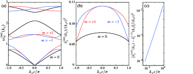
Figure 2: (Color online) (a) Phonon energy dispersion in a Te-like chiral lattice. Different CAM subspaces are distinguished by color. (b) $\lambda_{1}^{(m)}(k_{z})/(k_{z}c)^{2}$. (c) Scaling of the splitting $\bigl{|}\lambda_{1}^{(+1)}(k_{z})-\lambda_{1}^{(-1)}(k_{z})\bigr{|}$. The slope indicates this scale as $k_{z}^{5}$.

There have been some discussions about a possibility of sound velocity splitting between the $m\mspace{-3.0mu}=\mspace{-3.0mu}\pm 1$ CAM subspaces[51]. However, if the velocity value were split in the $k_{z}\mspace{-3.0mu}=\mspace{-3.0mu}0$ limit, it would require a nonanalyticity of $\lambda_{1}^{(\pm 1)}(k_{z})$, which one can easily disprove. In each $m$ CAM subspace, $\mathsf{v}_{\mathrm{eff}}^{(m)}(k_{z})$ is a smooth function of $k_{z}$, and its three eigenvalues are well separated at $k_{z}\mspace{-3.0mu}=\mspace{-3.0mu}0$. These two mean that the perturbation in $k_{z}$ should have a nonvanishing convergence radius, and disprove the nonanalyticity. Numerical analysis of our data concludes $\lambda_{1}^{(\pm 1)}(k_{z})\mspace{-2.0mu}\sim\mspace{-2.0mu}u^{2}\mspace{1.0mu}k_{z}^{2}\pm w_{5}\mspace{1.0mu}k_{z}^{5}$ as shown in Fig. 2(b) and (c). As for phonon energy, this leads to the asymptotics $\omega_{1}^{(\pm 1)}(k_{z})\mspace{-2.0mu}\sim\mspace{-2.0mu}|k_{z}|\mspace{2.0mu}\bigl{[}u\pm(w_{5}/2u)\mspace{2.0mu}k_{z}^{3}\bigr{]}$ with the sound velocity $u$, and thus an energy splitting appears in the order $O(k_{z}^{4})$. Note that in more general models, corrections may start from a lower-order such as $O(k_{z}^{3})$, and then it leads to an energy splitting of $O(k_{z}^{2})$.

Energy splitting due to chiral structure is more evident for the optical modes ($\alpha\mspace{-3.0mu}=\mspace{-3.0mu}2,3$). It appears in the order $O(k_{z})$ as

$$\lambda_{\alpha}^{(m)}(k_{z})\sim\lambda_{\alpha}(0)\mspace{-2.0mu}+\mspace{-2.0mu}\varGamma_{\alpha}\mspace{2.0mu}k_{z}\mspace{2.0mu}m.$$ (6)

Its coefficient $\varGamma_{\alpha}$ is an important indicator that quantifies the effects of chiral structure on phonon dispersion, and we will call it splitting coefficient. Since $k_{z}$ is a polar vector element and $m$ is axial, the splitting coefficient $\varGamma_{a}$ needs to be a pseudo-scalar. It should change sign under $z$-plane mirror operation but remains invariant under time reversal. In order to see which parts of the chiral structure dominate $\varGamma_{\alpha}$’s, it is desirable to realize a smooth control of chiral lattice structure and how it affects the values of $\varGamma_{\alpha}$’s.

Such a control of lattice chirality and its handedness is actually accomplished by glueing a chiral crystal together with its mirror image, i.e., enantiomorph. In the present case, one realization is the lattice with the unit cell shown in Fig. 1(c), which we will call double-handed triple helix (DHTH). This contains three sublattice sites positioned at $\bm{r}_{l}$ in Eq. (1) but now with $\bm{s}_{l}\mspace{-3.0mu}=\mspace{-3.0mu}\delta\bm{a}_{l}$, and then two types of bonds are assigned for opposite windings $\bm{t}_{l,l\pm 1}\mspace{-3.0mu}=\mspace{-3.0mu}\bm{s}_{l\pm 1}\mspace{-2.0mu}-\mspace{-2.0mu}\bm{s}_{l}\mspace{-2.0mu}+\mspace{-2.0mu}\bm{a}_{3}$. While the deformation energy of the left-hand wound ($L$) bonds is given by Eq. (2) with this redefinition, the right-hand wound ($R$) bonds contribute its counterpart $\mathscr{V}_{R,1}\mspace{-3.0mu}=\mspace{-3.0mu}\!\sum_{\bm{r}_{l}}\bigl{[}\bm{d}(\bm{r}_{l})\mspace{-2.0mu}-\mspace{-2.0mu}\bm{d}(\bm{r}_{l}\mspace{-2.0mu}+\mspace{-2.0mu}\bm{t}_{l,l-1})\bigr{]}\cdot\mathsf{v}_{l,l-1}\bigl{[}\bm{d}(\bm{r}_{l})\mspace{-2.0mu}-\mspace{-2.0mu}\bm{d}(\bm{r}_{l}\mspace{-2.0mu}+\mspace{-2.0mu}\bm{t}_{l,l-1})\bigr{]}$. To realize a completely nonchiral limit, one sets as $\mathsf{v}_{l+1,l}\mspace{-3.0mu}=\mspace{-3.0mu}\mathsf{m}_{z}\mspace{2.0mu}\mathsf{v}_{l,l+1}\mspace{2.0mu}\mathsf{m}_{z}$ with the mirror operation $\mathsf{m}_{z}\mspace{-2.0mu}\equiv\mspace{-2.0mu}\mbox{diag }(1,1,-1)$, since $\bm{t}_{l+1,l}\mspace{-3.0mu}=\mspace{-3.0mu}-\mathsf{m}_{z}\mspace{2.0mu}\bm{t}_{l,l+1}$. In particular, $\hat{\mathsf{v}}\mspace{-2.0mu}\equiv\mspace{-2.0mu}\mathsf{v}_{0,2}$ is identical to $\mathsf{v}_{2,0}$ in Eq. (3) except for the plus sign for $\varDelta K$. However, in more general cases in which handedness cancellation is incomplete, the parameters $K_{jj}$ and $\varDelta K$ differ between $L$- and $R$-bonds, and henceforth, we will add the label $L$ or $R$ to distinguish them. As before, the symmetry constraint determines the stiffness matrix for the other bonds $\mathsf{v}_{0,2}\mspace{-3.0mu}=\mspace{-3.0mu}\mathsf{C}_{3}\mspace{2.0mu}\mathsf{v}_{1,0}\mspace{2.0mu}\mathsf{C}_{3}^{T}\mspace{-3.0mu}=\mspace{-3.0mu}\mathsf{C}_{3}^{T}\mspace{2.0mu}\mathsf{v}_{2,1}\mspace{2.0mu}\mathsf{C}_{3}$.

In a general DHTH lattice, the total deformation energy is $\mathscr{V}_{L,1}\mspace{-2.0mu}+\mspace{-2.0mu}\mathscr{V}_{R,1}$, and this leads to the dynamical matrix $\underline{V}_{L,1}(\bm{k})\mspace{-2.0mu}+\mspace{-2.0mu}\underline{V}_{R,1}(\bm{k})\mspace{2.0mu}\equiv\underline{V}(\bm{k})$. As before, we will concentrate on the case of $\bm{k}\mspace{-3.0mu}=\mspace{-3.0mu}(0,0,k_{z})$. Then, $\underline{V}_{R,1}(k_{z})\mspace{-3.0mu}=\mspace{-3.0mu}\underline{V}_{R,1}(0,0,k_{z})$ is given by modifying the form in Eq. (4): first replace $\bar{\mathsf{v}}$ by $\hat{\mathsf{v}}$, and then interchange $\mathsf{C}_{3}$ and $\mathsf{C}_{3}^{T}$, and lastly operate complex conjugation. Since this also commutes with $\underline{C}_{3}$ defined before, $\underline{V}_{R,1}(k_{z})$ is reduced to a $3\mspace{-1.0mu}\times\mspace{-1.0mu}3$ effective matrix $\mathsf{v}_{\mathrm{eff},R}^{(m)}(k_{z})\mspace{-3.0mu}=\mspace{-3.0mu}\mathsf{F}(\phi_{m}^{-})\mspace{2.0mu}\hat{\mathsf{v}}\mspace{4.0mu}\mathsf{F}(\phi_{m}^{-})$, while its counterpart is $\mathsf{v}_{\mathrm{eff},L}^{(m)}(k_{z})\mspace{-3.0mu}=\mspace{-3.0mu}\mathsf{F}(\phi_{m}^{+})\mspace{2.0mu}\bar{\mathsf{v}}\mspace{4.0mu}\mathsf{F}(\phi_{m}^{+})$. Here, $\phi_{m}^{\pm}\mspace{-2.0mu}\equiv\mspace{-2.0mu}k_{z}c\pm{\textstyle\frac{2m\pi}{3}}$ and it has a different factor of $k_{z}c$ from the one in Eq. (2) due to the redefinition of the bond vectors $\bm{t}_{l,l\pm 1}$. The total effective dynamical matrix is $\bar{\mathsf{v}}_{\mathrm{eff}}^{(m)}(k_{z})\mspace{-2.0mu}\equiv\mspace{-2.0mu}\mathsf{v}_{\mathrm{eff},L}^{(m)}(k_{z})\mspace{-2.0mu}+\mspace{-2.0mu}\mathsf{v}_{\mathrm{eff},R}^{(m)}(k_{z})$, and it is instructive to rewrite it into the following form

$$\bar{\mathsf{v}}_{\mathrm{eff}}^{(m)}\mspace{1.0mu}(k_{z})=\bar{\mathsf{v}}_{0}-\zeta^{\mspace{2.0mu}-m}\mspace{2.0mu}\mathsf{C}_{3}^{T}\mspace{2.0mu}\mathsf{v}_{s}(-p)\mspace{2.0mu}\mathsf{C}_{3}^{T}-\zeta^{\mspace{2.0mu}m}\mspace{2.0mu}\mathsf{C}_{3}\mspace{2.0mu}\mathsf{v}_{s}(p)\mspace{2.0mu}\mathsf{C}_{3},$$ (7)

where $p\mspace{-3.0mu}=\mspace{-3.0mu}k_{z}c$. The constant term is $\bar{\mathsf{v}}_{0}\mspace{-2.0mu}\equiv\mspace{-2.0mu}{\textstyle\frac{1}{2}}\mspace{2.0mu}\mbox{diag }\bigl{(}K_{11,+}\mspace{-4.0mu}\mspace{-2.0mu}+\mspace{-2.0mu}\mspace{-2.0mu}3K_{22,+},3K_{11,+}\mspace{-4.0mu}\mspace{-2.0mu}+\mspace{-2.0mu}\mspace{-2.0mu}K_{22,+},4K_{33,+}\mspace{-2.0mu}\bigr{)}\mspace{-2.0mu}+\mspace{-2.0mu}\varDelta K_{-}\mathsf{X}$ defined with $(\mathsf{X})_{\mu,\nu}\mspace{-2.0mu}\equiv\mspace{-2.0mu}\delta_{\mu,y}\delta_{\nu,z}\mspace{-2.0mu}+\mspace{-2.0mu}\delta_{\mu,z}\delta_{\nu,y}$ and the (anti-)symmetrized parameters $K_{jj,\pm}\mspace{-2.0mu}\equiv\mspace{-2.0mu}K_{jj,L}\pm K_{jj,R}$ and $\varDelta K_{\pm}\mspace{-2.0mu}\equiv\mspace{-2.0mu}\varDelta K_{L}\pm\varDelta K_{R}$. The $k_{z}$-dependence comes from $\mathsf{v}_{s}(p)\mspace{-3.0mu}=\mspace{-3.0mu}\cos p\mspace{2.0mu}\mathsf{v}_{+}\mspace{-2.0mu}+\mspace{-2.0mu}i\sin p\mspace{2.0mu}\mathsf{v}_{-}$ defined with $\mathsf{v}_{\pm}\mspace{-3.0mu}=\mspace{-3.0mu}\mbox{diag }\bigl{(}K_{11,\pm},K_{22,\pm},K_{33,\pm}\bigr{)}\mspace{-2.0mu}-\mspace{-2.0mu}\varDelta K_{\mp}\mathsf{X}$. Note that $\mathsf{v}_{s}(p)$ is not hermitian, but has the relation $\mathsf{v}_{s}(-p)\mspace{-3.0mu}=\mspace{-3.0mu}\mathsf{v}_{s}(p)^{*}$. As in the previous case of single helix, the time reversal symmetry leads to the relation $\bar{\mathsf{v}}_{\mathrm{eff}}^{(-m)}(-k_{z})\mspace{-3.0mu}=\mspace{-3.0mu}\bar{\mathsf{v}}_{\mathrm{eff}}^{(m)}(k_{z})^{*}$, and this guarantees the energy degeneracy of chiral phonons $\omega_{\alpha}^{(-m)}(-k_{z})\mspace{-3.0mu}=\mspace{-3.0mu}\omega_{\alpha}^{(m)}(k_{z})$, in general DHTH lattices as shown in Fig. 3. The degeneracy at the BZ boundary $k_{z}\mspace{-3.0mu}=\mspace{-3.0mu}\pm k_{0}$ differs from the behavior in Fig. 2(a). As the DHTH lattice is now symmorphic, there holds the relation $\bar{\mathsf{v}}_{\mathrm{eff}}^{(m)}(k_{0})\mspace{-3.0mu}=\mspace{-3.0mu}\bar{\mathsf{v}}_{\mathrm{eff}}^{(m)}(-k_{0})\mspace{-3.0mu}=\mspace{-3.0mu}\bar{\mathsf{v}}_{\mathrm{eff}}^{(-m)}(\pm k_{0})^{*}$, and this leads to the degeneracy $\omega_{\alpha}^{(+1)}(k_{0})\mspace{-3.0mu}=\mspace{-3.0mu}\omega_{\alpha}^{(+1)}(-k_{0})\mspace{-3.0mu}=\mspace{-3.0mu}\omega_{\alpha}^{(-1)}(\pm k_{0})$. Note that when $\mathscr{V}_{R,1}$ is set to zero, the system is reduced to decoupled three copies of a Te-like lattice but their lattice constant $c$ is tripled.

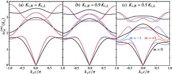
Figure 3: (Color online) Phonon energy dispersion in the DHTH lattice. The ratio $K_{i,R}/K_{i,L}$ is common for all $i$’s. The $m\mspace{-3.0mu}=\mspace{-3.0mu}\pm 1$ CAM modes are degenerate in (a).

It is important to examine the nonchiral limit where the right-handed part is a precise mirror image of the left-handed part. In this case, the antisymmetrized parameters vanish ($K_{jj,-}\mspace{-3.0mu}=\mspace{-3.0mu}\varDelta K_{-}\mspace{-3.0mu}=\mspace{-3.0mu}0$), and this leads to the special symmetries that $\mathsf{v}_{s}(-p)\mspace{-3.0mu}=\mspace{-3.0mu}\mathsf{m}_{z}\mspace{2.0mu}\mathsf{v}_{s}(p)\mspace{2.0mu}\mathsf{m}_{z}$ and $\bar{\mathsf{v}}_{0}$ is a diagonal matrix. Combining them with the property $[\mathsf{C}_{3}^{\pm 1},\mspace{2.0mu}\mathsf{m}_{z}]\mspace{-3.0mu}=\mspace{-3.0mu}0$, it is easy to show $\bar{\mathsf{v}}_{\mathrm{eff}}^{(m)}(-k_{z})\mspace{-3.0mu}=\mspace{-3.0mu}\mathsf{m}_{z}\mspace{2.0mu}\bar{\mathsf{v}}_{\mathrm{eff}}^{(m)}(k_{z})\mspace{2.0mu}\mathsf{m}_{z}$. Together with the chiral symmetry, this leads to the degeneracy of phonon energy dispersion between the opposite CAM modes, $\omega_{\alpha}^{(m)}(k_{z})\mspace{-3.0mu}=\mspace{-3.0mu}\omega_{\alpha}^{(-m)}(k_{z})$. Note that this additional symmetry is specific to the nonchiral limit.

Finally, let us evaluate the energy splitting for the opposite CAM modes, which determines the splitting coefficient $\varGamma_{\alpha}$ introduced before. We can calculate this by following the standard procedure of the first-order perturbation in $k_{z}$. Let $\vec{d}_{\alpha}^{\mspace{4.0mu}(m)}$ denote the 9-dimensional eigenvectors of $\underline{V}(k_{z}\!=\!0)$ in the CAM subspaces $m\!=\!\pm 1$. They satisfy the relation $\vec{d}_{\alpha}^{\mspace{4.0mu}(-1)}\mspace{-3.0mu}=\mspace{-3.0mu}[\vec{d}_{\alpha}^{\mspace{4.0mu}(+1)}]^{\,*}$. We can show immediately $m\mspace{2.0mu}\varGamma_{\alpha}\mspace{-3.0mu}=\mspace{-3.0mu}\langle\vec{d}_{\alpha}^{\mspace{4.0mu}(m)}\mspace{2.0mu}|\mspace{2.0mu}\underline{D}_{z}\mspace{2.0mu}|\mspace{2.0mu}\vec{d}_{\alpha}^{\mspace{4.0mu}(m)}\rangle$ with $\underline{D}_{z}\equiv\bigl{[}d\underline{V}(k_{z})/dk_{z}\bigr{]}_{k_{z}=0}$, and this new matrix is represented as

$$\underline{D}_{z}=-i\left[\begin{array}[]{@{\hs{2pt}}c@{\hs{4pt}}c@{\hs{4pt}}c@{\hs{2pt}}}\hskip 2.0pt\lx@intercol\hfil\mathsf{0}\hfil\hskip 4.0&z_{01}\mspace{2.0mu}\mathsf{C}_{3}^{T}\mspace{2.0mu}\mathsf{v}_{-}\mspace{2.0mu}\mathsf{C}_{3}\hfil\hskip 4.0&z_{02}\mspace{2.0mu}\mathsf{v}_{-}\hfil\hskip 2.0\\[2.0pt] \hskip 2.0pt\lx@intercol\hfil z_{10}\mspace{2.0mu}\mathsf{C}_{3}^{T}\mspace{2.0mu}\mathsf{v}_{-}\mspace{2.0mu}\mathsf{C}_{3}\hfil\hskip 4.0&\mathsf{0}\hfil\hskip 4.0&z_{12}\mspace{2.0mu}\mathsf{C}_{3}\mspace{2.0mu}\mathsf{v}_{-}\mspace{2.0mu}\mathsf{C}_{3}^{T}\hfil\hskip 2.0\\[2.0pt] \hskip 2.0pt\lx@intercol\hfil z_{20}\mspace{2.0mu}\mathsf{v}_{-}\hfil\hskip 4.0&z_{21}\mspace{2.0mu}\mathsf{C}_{3}\mspace{2.0mu}\mathsf{v}_{-}\mspace{2.0mu}\mathsf{C}_{3}^{T}\hfil\hskip 4.0&\mathsf{0}\hfil\hskip 2.0\end{array}\right].$$ (8)

Here, $z_{ll^{\prime}}$ is the $z$-component of the bond vector $\bm{t}_{ll^{\prime}}$, and $z_{l^{\prime}l}\mspace{-3.0mu}=\mspace{-3.0mu}-z_{ll^{\prime}}$. Thus, this hermitian matrix $\underline{D}_{z}$ is pure imaginary and similar to a current in the sense that it changes sign under each of time reversal and space inversion operations. It is possible to separate the pseudo-scalar part $\varGamma_{a}$ alone by combining the CAM operator:

$$\varGamma_{\alpha}\mspace{-3.0mu}=\mspace{-3.0mu}\langle\vec{d}_{\alpha}^{\mspace{4.0mu}(m)}\mspace{2.0mu}|\mspace{2.0mu}\underline{\varGamma}\mspace{2.0mu}|\mspace{2.0mu}\vec{d}_{\alpha}^{\mspace{4.0mu}(m)}\rangle,\ \ \mbox{with }\underline{\varGamma}\equiv\underline{L}_{z}\,\underline{D}_{z}.$$ (9)

Note that $\underline{\varGamma}$ is real symmetric, since $\underline{L}_{z}$ and $\underline{D}_{z}$ commute. Thus, this $\underline{\varGamma}$ is the operator that defines the chirality (handedness) of the system. We skip the detail of calculating the matrix element $\varGamma_{\alpha}$ and show the final result:

$$\varGamma_{\alpha}={\textstyle\frac{\sqrt{3}}{2}}\,\Bigl{[}\bigl{(}1\mp\cos\beta\bigr{)}K_{33,-}\mspace{-2.0mu}-\mspace{-2.0mu}{\textstyle\frac{1}{2}}\bigl{(}1\pm\cos\beta\bigr{)}\bigl{(}K_{11,-}\mspace{-2.0mu}+\mspace{-2.0mu}K_{22,-}\bigr{)}\Bigr{]},$$ (10)

where the upper and lower signs are for $\alpha\mspace{-3.0mu}=\mspace{-3.0mu}2$ and 3, respectively, and $\beta\mspace{-2.0mu}\equiv\mspace{-2.0mu}\tan^{-1}\bigl{[}\sqrt{8}\mspace{2.0mu}\varDelta K_{-}(K_{11,+}\mspace{-2.0mu}\mspace{-2.0mu}+\mspace{-2.0mu}K_{22,+}\mspace{-2.0mu}\mspace{-2.0mu}-\mspace{-2.0mu}2K_{33,+})^{-1}\bigr{]}$. It is interesting that they satisfy the simple sum rule $\varGamma_{2}\mspace{-2.0mu}+\mspace{-2.0mu}\varGamma_{3}\mspace{-3.0mu}=\mspace{-3.0mu}\sqrt{3}\mspace{2.0mu}\bigl{[}K_{33,-}\mspace{-2.0mu}-\mspace{-2.0mu}{\textstyle\frac{1}{2}}\bigl{(}K_{11,-}\mspace{-2.0mu}+\mspace{-2.0mu}K_{22,-}\bigr{)}\bigr{]}\mspace{-2.0mu}\equiv\mspace{-2.0mu}\varGamma_{s}$, which is also represented in terms of the tensor’s principle values as $\varGamma_{s}\mspace{-3.0mu}=\mspace{-3.0mu}{\textstyle\frac{1}{4}}(K_{2,-}\mspace{-2.0mu}+\mspace{-2.0mu}K_{3,-}\mspace{-2.0mu}-\mspace{-2.0mu}2K_{1,-})\mspace{-2.0mu}+\mspace{-2.0mu}{\textstyle\frac{3}{4}}(K_{3,-}\mspace{-2.0mu}-\mspace{-2.0mu}K_{2,-})\cos 2\theta$, where $\theta$ is the effective bond angle introduced before for defining $\mathsf{v}_{2,0}$. This $\varGamma_{s}$ is completely determined by the antisymmetrized parameters (i.e., imbalance between the left- and right-handed parts), and independent of the symmetrized parameters (i.e., common factors in the two parts). Therefore, we may consider $\varGamma_{s}$ as the most fundamental indicator characterizing the effects of chiral structure on phonon dispersion. The parameter $\beta$ determines how the sum $\varGamma_{s}$ is distributed between the two optical modes. Note that one can apply these results to the systems with one chiral part alone such as Te lattice, and in those cases $K_{jj,+}\mspace{-3.0mu}=\mspace{-3.0mu}|K_{jj,-}|$ and $|\varDelta K_{+}|\mspace{-3.0mu}=\mspace{-3.0mu}|\varDelta K_{-}|$. It is clear that $\varGamma_{s}$ changes its sign upon a reversal of lattice handedness.

It is important to notice that one can represent this indicator as an averaged uniaxial anisotropy $Q_{u}(\mathsf{v})\mspace{-3.0mu}=\mspace{-3.0mu}\!{\textstyle\frac{\sqrt{3}}{4}}\,\mbox{Tr}\mspace{2.0mu}[(1\mspace{-2.0mu}-\mspace{-2.0mu}3\mathsf{m}_{z})\,\mathsf{v}]$ of the local stiffness matrices weighted by the bond sign of handedness $h\mspace{-3.0mu}=\mspace{-3.0mu}+1$ for left and $-1$ for right bonds: $\varGamma_{s}\mspace{-3.0mu}=\mspace{-3.0mu}N^{-1}\sum_{\bm{R}}h(\bm{R})\,Q_{u}(\mathsf{v}(\bm{R}))$ with $N$ being the number of sites. $\bm{R}$ denotes a bond center position measured from the nearest chiral axis, and if multiple $\mathsf{v}$’s exist at the same $\bm{R}$, they should be all counted.

Since the splitting coefficients $\varGamma_{\alpha}$ are a kind of the “order parameters” of the chiral system, they belong to a nontrivial representation of the supergroup $D_{3h}$. Considering $\underline{L}_{z}$ and $\underline{D}_{z}$ in Eq. (9) belong to $A_{2}^{\prime}$ and $A_{2}^{\prime\mspace{-2.0mu}\prime}$, respectively, $\varGamma_{\alpha}$’s have the same symmetry as $m\cdot k_{z}$, i.e., $A_{2}^{\prime}\otimes A_{2}^{\prime\mspace{-2.0mu}\prime}\mspace{-3.0mu}=\mspace{-3.0mu}A_{1}^{\prime\mspace{-2.0mu}\prime}$. In the language of cluster multipoles, they correspond to the pseudo-scalar (electric toroidal) multipoles of $G_{0}$ and $G_{u}$-type [5, 63], the latter of which gives the mono-axial anisotropy. A caution is necessary for the term “pseudo-scalar” in the systems without inversion or any mirror symmetries. It is instructive to elevate the system’s symmetry by supplementing generator(s) of mirror or inversion type. In our case, with the mirror $\mathsf{m}_{z}$ supplemented, the chiral point group $D_{3}$ is elevated to its nonchiral supergroup $D_{3h}$, which is the symmetry of the DHTH with the symmetric couplings $K_{j,R}\mspace{-3.0mu}=\mspace{-3.0mu}K_{j,L}$. Pseudo-scalars are defined as bases of its $A_{1}^{\prime\mspace{-2.0mu}\prime}$ representation, which changes sign under improper rotations and mirror operations. When the system is chiral ($K_{j,R}\neq K_{j,L}$), $\underline{\varGamma}$ falls into the identity representation $A_{1}$ of the $D_{3}$ point group, and gives a nonvanishing contribution to the CAM mode splitting. Similarly, in the cubic chiral systems, the lowest-order pseudo-scalar multipoles ($A_{1u}$, $A_{2}$, $A_{u}$ in the supergroup $O_{h}$, $T_{d}$, $T_{h}$) of $G_{0}$ and $G_{4}$-type[5, 63] induce a CAM splitting.

To summarize, we have developed a microscopic theory on the energy dispersion of chiral phonons within the harmonic approximation. Those chiral phonons are characterized by the crystal angular momentum $m\mspace{-3.0mu}=\mspace{-3.0mu}\pm 1$, and the splitting of their energy dispersions depending on $m$. This $k_{z}$-linear energy splitting in the optical modes is indicated by nonvanishing splitting coefficients $\varGamma_{\alpha}$. They are thus order parameters of the chiral system, belonging to the nontrivial $A_{1}^{\prime\mspace{-2.0mu}\prime}$ representation of the supergroup, and related to the $G_{0}$- and $G_{u}$-type electric toroidal multipoles (or $G_{4}$ type when the chiral system is cubic). Analyticity of the dynamical matrix in $\bm{k}$ enforces an identical value of sound velocity for their acoustic modes, and a splitting appears in the order of at least $k^{2}$ or higher. It is also important that stability of the equilibrium structure forbids the presence of antisymmetric interactions, because they otherwise violate the positivity of stiffness matrices. These constraints are crucial for modeling real materials in the first-principles phonon calculations. The splitting is much more visible in optical modes, and it starts from the order $O(k^{1})$. Its size is determined by the uniaxially anisotropic component of the stiffness matrices about the chiral axis. These fundamental findings of the present paper will provide further insights for elucidating the phonon and related phenomena in chiral systems.

The authors thank Jun-ichiro Kishine, Hiroyasu Matsuura, and Kazumasa Hattori for fruitful discussions. This research was supported by JSPS KAKENHI Grants Numbers JP21H01031 and 19K03752.

References

• [1] L. Kelvin, in Baltimore Lectures on Molecular Dynamics and the Wave Theory of Light (C. J. Clay and Sons, London, 1904).
• [2] G. H. WagnieΕ•e, On Chirality and the Universal Asymmetry: Reflections on Image and Mirror Image (Wiley-VCH, Weinheim, 2007).
• [3] L. D. Barron, Molecular Light Scattering and Optical Activity, 2nd ed. (Cambridge University Press, Cambridge, England, 2004).
• [4] R. Oiwa and H. Kusunose, Phys. Rev. Lett. 129, 116401 (2022).
• [5] J. Kishine, H. Kusunose, and H. M. Yamamoto, , Isr. J. Chem. 62, e202200049 (2022).
• [6] E. Hendry, T. Carpy, J. Johnston, M. Popland, R. V. Mikhaylovskiy, A. J. Lapthorn, S. M. Kelly, L. D. Barron, N. Gadegaard, and M. Kadodwala, Nat. Nanotechnol. 5, 783 (2010).
• [7] M. Kuwata-Gonokami, N. Saito, Y. Ino, M. Kauranen, K. Jefimovs, T. Vallius, J. Turunen, and Y. Svirko, Phys. Rev. Lett. 95, 227401 (2005).
• [8] C. Kelly, D. A. MacLaren, K. McKay, A. McFarlane, A. S. Karimullah, N. Gadegaard, L. D. Barron, S. Franke-Arnold, F. Crimin, J. B. GΓΆtte, S. M. Barnett, and M. Kadodwala, Nat. Commun. 11, 5169 (2020).
• [9] G. L. J. A. Rikken, C. Strohm, and P. Wyder, Phys. Rev. Lett. 89, 133005 (2002).
• [10] Y. Tokura and N. Nagaosa, Nat. Commun. 9, 3740 (2018).
• [11] T. Furukawa, Y. Shimokawa, K. Kobayashi, and T. Itou, Nat. Commun. 8, 954 (2017).
• [12] T. Yoda, T. Yokoyama, and S. Murakami, Nano Lett. 18, 916 (2018).
• [13] S. MΓΌhlbauer, B. Binz, F. Jonietz, C. Pfleiderer, A. Rosch, A. Neubauer, R. Georgii, and P. BΓΆni, Science 323, 915 (2009).
• [14] Y. Togawa, T. Koyama, K. Takayanagi, S. Mori, Y. Kousaka, J. Akimitsu, S. Nishihara, K. Inoue, A.S. Ovchinnikov, and J. Kishine, Phys. Rev. Lett. 108, 107202 (2012).
• [15] J. Kishine and A. S. Ovchinnikov, Solid State Physics 66 (Elsevier, 2015).
• [16] Y. Togawa, Y. Kousaka, K. Inoue, and J. Kishine, J. Phys. Soc. Jpn. 85, 112001 (2016).
• [17] B. GΓΆhler, V. Hamelbeck, T.Z. Markus, M. Kettner, G.F. Hanne, Z. Vager, R. Naaman, and H. Zacharias, Science 331, 894 (2011).
• [18] R. Naaman and D. H. Waldeck, J. Phys. Chem. Lett. 3, 2178 (2012).
• [19] R. Naaman, Y. Paltiel, and D. H. Waldeck, Nat. Rev. Chem. 3, 250 (2019).
• [20] R. Naaman, Y. Paltiel, and D. H. Waldeck, J. Phys. Chem. Lett. 11, 3660 (2020).
• [21] F. Evers, A. Aharony, N. Bar-Gill, O. Entin-Wohlman, P. HedegΓ₯rd, O. Hod, P. Jelinek, G. Kamieniarz, M. Lemeshko, K. Michaeli, V. Mujica, R. Naaman, Y. Paltiel, S. Rafaely-Abramson, O. Tal, J. Thijssen, M. Thoss, J. M. van Ruitenbeek, L. Venkataraman, D. H. Waldeck, B. Yan, and L. Kronik, Adv. Mater. 34, 2106629 (2022).
• [22] A. Inui, R. Aoki, Y. Nishiue, K. Shiota, Y. Kousaka, H. Shishido, D. Hirobe, M. Suda, J. Ohe, J. Kishine, H. M. Yamamoto, and Y. Togawa, Phys. Rev. Lett. 124, 166602 (2020).
• [23] Y. Nabei, D. Hirobe, Y. Shimamoto, K. Shiota, A. Inui, Y. Kousaka, Y. Togawa, and H. M. Yamamoto, Appl. Phys. Lett. 117, 052408 (2020).
• [24] K. Shiota, A. Inui, Y. Hosaka, R. Amano, Y. Ōnuki, M. Hedo, T. Nakama, D. Hirobe, J. Ohe, J. Kishine, H. M. Yamamoto, H. Shishido, and Y. Togawa, Phys. Rev. Lett. 127, 126602 (2021).
• [25] K. de Boer, A. P. J. Jansen, R. A. van Santen, G. W. Watson, and S. C. Parker, Phys. Rev. B 54, 826 (1996).
• [26] P. Ghosh, J. Bhattacharjee, and U. V. Waghmare, J. Phys. Chem. C 112, 983 (2008).
• [27] A. S. Pine, Phys. Rev. B 2, 2049 (1970).
• [28] A. S. Pine and G. Dresselhaus, Phys. Rev. B 4, 356 (1971).
• [29] W. D. Teuchert and R. Geick, Phys. Stat. Sol. 61, 123 (1974).
• [30] R.M.Β Martin and G.Β Lucovsky, Phys. Rev. B 13, 1383 (1976).
• [31] H. Zhu, J. Yi, M.-Y. Li, J. Xiao, L. Zhang, C.-W. Yang, R. A. Kaindl, L.-J. Li, Y. Wang, and X. Zhang, Science 359, 579 (2018).
• [32] H. Chen, W. Wu, J. Zhu, Z. Yang, W. Gong, W. Gao, S. A. Yang, and L. Zhang, Nano Lett. 22, 1688 (2022).
• [33] S. V. Vonsovskii and M. S. Svirskii, Sov. Phys. Solid State 3, 1568 (1962).
• [34] L. Zhang and Q. Niu, Phys. Rev. Lett. 112, 085503 (2014).
• [35] Y. Tatsumi, T. Kaneko, and R. Saito, Phys. Rev. B 97, 195444 (2018).
• [36] T. Zhang and S. Murakami, Phys. Rev. Research 4, L012024 (2022).
• [37] H. Komiyama, T. Zhang, and S. Murakami, Phys. Rev. B 106, 184104 (2022).
• [38] Crystal angular momentum is often called as pseudo-angular momentum as well.
• [39] D. A. Garanin and E. M. Chudnovsky, Phys. Rev. B 92, 024421 (2015).
• [40] J. J. Nakane and H. Kohno, Phys. Rev. B 97, 174403 (2018).
• [41] S. Streib, H. Keshtgar, and G. E. W. Bauer, Phys. Rev. Lett. 121, 027202 (2018).
• [42] J. Holanda, D. S. Maior, A. Azevedo, and S. M. Rezende, Nat. Phys. 14, 500 (2018).
• [43] S. C. Guerreiro and S. M. Rezende, Phys. Rev. B 92, 214437 (2015).
• [44] D. M. Juraschek and N. A. Spaldin, Phys. Rev. Mater. 3, 064405 (2019).
• [45] D. Yao and S. Murakami, Phys. Rev. B 105, 184412 (2022).
• [46] K. Ishito, H. Mao, Y. Kousaka, Y. Togawa, S. Iwasaki, T. Zhang, S. Murakami, J. Kishine, and T. Satoh, Nat. Phys. (2022). https://doi.org/10.1038/s41567-022-01790-x
• [47] A. Kato, H. M. Yamamoto, and J. Kishine, Phys. Rev. B 105, 195117 (2022).
• [48] S. K. Bose and E. S. Zijlstra, Physica C 432, 173 (2005).
• [49] H. Q. Yuan, D. F. Agterberg, N. Hayashi, P. Badica, D. Vandervelde, K. Togano, M. Sigrist, and M. B. Salamon, Phys. Rev. Lett. 97, 017006 (2006).
• [50] M. Nishiyama, Y. Inada, and G. Zheng, Phys. Rev. Lett. 98, 047002 (2007).
• [51] D. L. Portigal and E. Burstein, Phys. Rev. 170, 673 (1968).
• [52] J. Kishine, A. S. Ovchinnikov, and A. A.Tereshchenko, Phys. Rev. Lett. 125, 245302 (2020).
• [53] A. C. Eringen, Microcontinuum Field Theories (Springer, 2012).
• [54] W. Nowacki, Theory of Asymmetric Elasticity (Pergamon Press, 1985).
• [55] Y. Chen, M. Kadic, and M. Wegener, Nat. Commun. 12, 3278 (2021).
• [56] A. Togo and I. Tanaka, Scripta Materialia, 108, 1 (2015).
• [57] ABINIT homepage, https://www.abinit.org/
• [58] Phonon website, β€œVisualize phonon vibrational modes”, https://henriquemiranda.github.io/phononwebsite/index.html
• [59] C. Adenis, V. Langer, and O. Lindqvist, Acta Cryst. C 45, 941 (1989).
• [60] I. Patzak, Z. Metallkunde 47, 418 (1956).
• [61] R. GonzΓ‘lez-HernΓ‘ndez, E. Tuiran, and B. Uribe, Phys. Rev. Mater. 4, 124203 (2020).
• [62] R. GonzΓ‘lez-HernΓ‘ndez, E. Tuiran, and B. Uribe, Phys. Rev. B 103, 235143 (2021).
• [63] S.Β Hayami, M.Β Yatsushiro, Y.Β Yanagi, and H.Β Kusunose, Phys. Rev. B 98, 165110 (2018).