Using Host Galaxy Photometric Redshifts to Improve Cosmological Constraints with Type Ia Supernova in the LSST Era

Abstract

We perform a rigorous cosmology analysis on simulated type Ia supernovae (SN Ia) and evaluate the improvement from including photometric host-galaxy redshifts compared to using only the “$z_{\rm spec}$” subset with spectroscopic redshifts from the host or SN. We use the Deep Drilling Fields (${\sim}50$ deg²) from the Photometric LSST Astronomical Time-Series Classification Challenge (PLAsTiCC), in combination with a low-$z$ sample based on Data Challenge2 (DC2). The analysis includes light curve fitting to standardize the SN brightness, a high-statistics simulation to obtain a bias-corrected Hubble diagram, a statistical+systematics covariance matrix including calibration and photo-$z$ uncertainties, and cosmology fitting with a prior from the cosmic microwave background. Compared to using the $z_{\rm spec}$ subset, including events with SN+host photo-$z$ results in i) more precise distances for $z>0.5$, ii) a Hubble diagram that extends 0.3 further in redshift, and iii) a 50% increase in the Dark Energy Task Force figure of merit (FoM) based on the $w_{0}w_{a}$CDM model. Analyzing 25 simulated data samples, the average bias on $w_{0}$ and $w_{a}$ is consistent with zero. The host photo-$z$ systematic of 0.01 reduces FoM by only 2% because i) most $z<0.5$ events are in the $z_{\rm spec}$ subset, ii) the combined SN+host photo-$z$ has $\times 2$ smaller bias, and iii) the anti-correlation between fitted redshift and color self corrects distance errors. To prepare for analysing real data, the next SNIa-cosmology analysis with photo-$z$’s should include non SN-Ia contamination and host galaxy mis-associations.

I Introduction

Since the discovery of cosmic acceleration (Perlmutter et al., 1999; Riess et al., 1998) using Type Ia supernovae (SNe Ia), this geometric probe has provided unique constraints on the dark energy equation of state (EOS) today, $w_{0}$, and its variation with cosmic time, $w_{a}$ (Linder, 2003; Chevallier and Polarski, 2001). The most precise measurements of the dark energy EOS have been based on ${\sim}1000$ spectroscopically confirmed SN samples with spectroscopic redshifts from the SN or host-galaxy (Betoule et al., 2014; Scolnic et al., 2018; Abbott et al., 2019; Brout et al., 2022).

Over the next decade, much larger SN samples are expected from the Vera C. Rubin Observatory and Legacy Survey of Space and Time (LSST) and the Nancy Grace Roman Space Telescope. Spectroscopic resources will be capable of observing only a small fraction of the discovered SNe. To make full use of these future samples in cosmology analyses, well developed methods have been used for photometric classification using broadband photometry (Lochner et al., 2016; Möller and de Boissière, 2020). A photometric redshift method using the SN+host galaxy photo-$z$ has been proposed (Kessler et al., 2010; Palanque-Delabrouille et al., 2010; Roberts et al., 2017), but a rigorous SNIa-cosmology analysis with photo-$z$’s has not been performed.

To analyse SN Ia samples with contamination from other SN types, the “BEAMS” framework was developed to rigorously use the photometric classification probabilities (Kunz et al., 2007; Hlozek et al., 2012). The BEAMS framework, combined with photometric classification, was first used to obtain SNIa-cosmology results from Pan-Starrs1 data (Jones et al., 2018). An extension to BEAMS, “BEAMS with Bias Corrections” (BBC; Kessler and Scolnic (2017); hereafter KS17), was used in Jones et al. (2018) and is currently used in the analysis of data from the Dark Energy Survey (Vincenzi et al., 2022).

To analyze SN Ia samples using photometric redshifts, Kessler et al. (2010) and Palanque-Delabrouille et al. (2010) extended the SALT2 light curve fitting framework (Guy et al., 2007) to include redshift as an additional fitted parameter, and to use the host-galaxy photo-$z$ as a prior. Dai et al. (2018) analyzed a simulated LSST sample including SNe Ia and SNe CC, and applied both photometric classification (but not BEAMS) and the SALT2 photo-$z$ method. They fit the resulting Hubble diagram with a flat-$\Lambda$CDM model and recovered unbiased $\Omega_{\rm M}$ with a statistical precision of $0.008$. Using data from the Dark Energy Survey (DES), Chen et al. (2022) performed a photo-$z$ analysis using a subset of ${\sim}100$ SNe Ia hosted by redMagic galaxies for which both photometric and spectroscopic redshifts are available. Fitting their Hubble diagram with a flat $w$CDM model, they find a $w$-difference of 0.005 between using spectroscopic and photometric (redMagic) redshifts. Finally, Linder and Mitra (2019); Mitra and Linder (2021) evaluated the impact of photometric redshifts for LSST using a Fisher matrix approximation that does not include light curve fitting or bias corrections. They concluded that for $z<0.2$, spectroscopic redshifts are necessary for robust cosmology measurements.

A hierarchical Bayesian methodology (Roberts et al., 2017, zBEAMS) has been proposed to combine photometric classification (BEAMS), photometric host-galaxy redshifts, and incorrect host-galaxy assignments. This method has been validated on a toy simulation of SN distances with random fluctuations, but the analysis does not include light curve fitting, bias corrections, or systematic uncertainties.

Here we present a rigorous SNIa-cosmology analysis on simulated LSST data that includes host galaxy photo-$z$’s. We use these photo-$z$s to include more distant SNe that would otherwise be excluded in a spectroscopically confirmed sample, and we evaluate the impact of including these additional SNe in the cosmology analysis. Our simulation is based on the cadence of the Deep Drilling Fields (DDF) from the Photometric LSST Astronomical Time-series Classification Challenge (PLAsTiCC, Kessler et al., 2019a, see sec. §III.1), combined with a low-$z$ sample based on the cadence of the Wide Fast Deep (WFD) fields. Our end-to-end analysis includes light curve fitting, simulated bias corrections applied with BBC, a covariance matrix that includes systematic uncertainties, and fitting a bias-corrected Hubble diagram for cosmological parameters. We examine the $w$CDM and $w_{0}w_{a}$CDM models.

We adopt the photo-$z$ method from Kessler et al. (2010), and we use the host-galaxy photo-$z$ as a prior. To focus on photo-$z$ issues, we simulate SNe Ia only (without contamination) and assume that all host-galaxies are correctly identified. Therefore, the BEAMS formalism is not used in the analysis. We use science codes from the publicly available SuperNova ANAlysis software package SNANA (Kessler et al., 2009), and we use the cosmology-analysis workflow from Pippin (Hinton and Brout, 2020).

This paper is presented as follows. In sec. II, we briefly review LSST and the Dark Energy Science Collaboration. Sec III describes the simulated data sample and Sec. IV describes the cosmology analysis. Results are presented in sec. V and we conclude in Sec. VI.

II Overview of LSST and Dark Energy Science Collaboration

LSST is a ground-based stage IV dark energy survey program (Cahn, 2009; Ivezić et al., 2019). It is expected to become operational in $2023$, and will discover millions of supernova over the 10 year survey duration. The Simonyi Survey optical Telescope at the Rubin Observatory includes an $8.4~{}m$ mirror and a state-of-the-art $3200$ megapixel camera ($9.6$ deg² FoV) that will provide the deepest and the widest views of the Universe with unprecedented quality. LSST will observe nearly half the night sky every week to a depth of $24^{th}$ magnitude in the six filter bands ($ugrizy$) spanning wavelengths from ultra-violet to near-infrared.

The Dark Energy Science Collaboration (DESC) is an analysis team with nearly 1,000 members, and their goal is to make numerous high accuracy measurements of fundamental cosmological parameters using data from LSST. Prior to first light, DESC has implemented data challenges as a strategy to continuously develop analysis pipelines. This photo-$z$ analysis within the Time Domain working group leverages two previous challenges: 1) a transient classification challenge (PLAsTiCC), and 2) an image-processing challenge (DC2: LSST Dark Energy Science Collaboration et al.(2021)LSST Dark Energy Science Collaboration (LSST DESC), Abolfathi, Alonso, Armstrong, Aubourg, Awan, Babuji, Bauer, Bean, Beckett et al. (LSST DESC); Sánchez et al. (2021)). An updated PLAsTiCC challenge, with several new models and transient-host correlations (Lokken et al., 2022), is under development to test early classification and to test processing large numbers of detection “alerts” expected from the Rubin Observatory.

III Simulated Data

We do not work with simulated images and thus we don’t run the LSST difference imaging analysis (DIA) based on Alard and Lupton (1998). Instead, we simulate SN Ia light curves corresponding to the output of DIA, and calibrated to the AB magnitude system (Fukugita et al., 1996). Following PLAsTiCC (Kessler et al., 2019a; Hložek et al., 2020), we use the cadence and observing properties from MINION1016 and we include a host galaxy photometric redshift and rms uncertainty based on Graham et al. (2018, hereafter G18), but we do not model correlations between the SNe and host galaxy properties. PLAsTiCC was designed to motivate the development of classification algorithms for photometric light curves from transients discovered by LSST.

PLAsTiCC included two LSST observing strategies: 1) five Deep-Drilling-Fields (DDF), covering ${\sim}50$ deg², that are revisited frequently and hence correspond to areas with enhanced depth and 2) the Wide-Fast-Deep (WFD) covering a majority of the southern sky ($18000$ deg²). We simulate a high-$z$ sample using DDF and co-add the nightly observations within each band (sec. III.1). Since the PLAsTiCC DDF data has limited statistics at low redshifts, we compliment the PLAsTiCC data with a spectroscopically confirmed low-$z$ sample (sec. III.2) based on the wide-fast-deep (WFD) cadence used in DC2.

Rather than using the publicly available PLAsTiCC data, we regenerate the DDF simulation because our analysis needs a much larger sample for bias corrections that is not publicly available. We have verified that our new sample is statistically equivalent to the public data by comparing distributions of redshift, color and stretch. Our simulation does not include contamination from core collapse and peculiar SNe, nor DIA artifacts such as catastrophic flux outliers, PSF model errors, and non-linearites.

The simulation process adapted in this analysis is described in depth in Kessler et al. (2019b). To accurately measure biases on cosmological parameters, 25 statistically independent simulated data samples are generated and each sample is analyzed seperately.

A summary of average simulation statistics is shown in Table 1. For the high-z sample, the number of generated events ($N_{\rm gen}$ column of Table 1) is computed from the measured volumetric rate, duration of the survey, and $50$ deg² area of DDF. For low-$z$, $N_{\rm gen}$ is arbitrarily chosen such that the number of events after selection requirements is roughly $500$, which is about $\sim 10\%$ of the high-z statistics. Examples of simulated light curves at different redshifts are shown by the black circles in Fig. 1.

.

Figure 1: Sample simulated light curves (calibrated flux vs. $T_{\rm OBS}=\rm MJD-t_{0}$) for redshifts spanning $z\sim[0-1.2]$. Each column shows a light curve from a single event in each of the six LSST optical pass band filters $u,g,r,i,z,y$. Left most column ($z=0.05$) is from low-$z$ (WFD); the remaining events are from high-$z$ (DDF). The smooth curves are fits from the SALT2 model, and each color corresponds to a different passband

Table 1: Summary of simulations statistics.

	$z$- range	$N_{\rm gen}$	$N_{\rm gen}$	After	Selection Cuts:
		total	trigger	$z_{\rm spec}$	full sample
Low-$z$	$0.01-0.08$	$4200$	$696$	$539$	$539$
High-$z$	$0.03-1.55$	$41819$	$12808$	$1482$	$4873$

III.1 High-$z$ data : PLAsTiCC

The original PLAsTiCC simulation covers the first three years of LSST with 18 models that include both extragalactic and galactic transients. For this analysis, we simulate only SNe Ia using the SALT2 model (Guy et al., 2007). This model includes measured populations of stretch and color from Scolnic and Kessler (2016) with stretch- and color-luminosity parameters ($\alpha=0.14$, $\beta=3.1)$, an intrinsic scatter of the model SED, and a near-infrared extension (Pierel et al., 2018) to include the $i,z,y$ band wavelength range. Correlations between SNe and host-galaxy mass are not included. Next, the model SED is modified to account for cosmic expansion ($\Omega_{\rm M}=0.315$, $w=-1$, flatness) redshift, and Galactic extinction from Schlafly and Finkbeiner (2011). Filter passbands are used to compute broadband fluxes at epochs determined by the DDF cadence from OpSim (Delgado et al., 2014; OpS, 2016; Reuter et al., 2016), and observing conditions (zero-point, PSF and sky noise) are used to model flux uncertainties. The $5\sigma$ limiting magnitudes for each of the $ugrizy$ passbands are listed in Table 2 for both the low-$z$ and the high-$z$ samples. We adopt the detection efficiency vs. signal-to-noise ratio (SNR) from the DC2 analysis as shown in Fig. 9 of Sánchez et al. (2021). The simulated trigger selects events with two detections separated by at least 30 minutes.

Following PLAsTiCC, we define a “$z_{\rm spec}$” sample consisting of two subsets of events with accurate spectroscopic redshifts ($\sigma_{z}\sim 10^{-5}$). The first subset assumes an accurate redshift from spectroscopically confirmed events based on a forecast of the performance for the 4-metre Multi-Object Spectroscopic Telescope spectrograph (4MOST hereafter, de Jong et al., 2019) that is under construction by the European Southern Observatory (ESO). 4MOST is expected to begin operation in $2023$ (similar to the LSST timeline) and is located at a latitude similar to that of the Rubin observatory in Chile. The second subset includes photometrically identified events with an accurate host galaxy redshift using 4MOST. The second subset has about $\sim 60$% more events than the first subset, and each subset is treated identically in the analysis. The simulated efficiency vs. redshift for each $z_{\rm spec}$ subset is shown in Fig. 2.

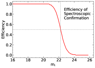
(a)

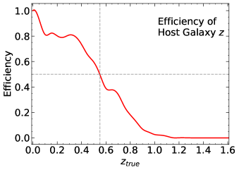
(b)

Figure 2: For DDF, Top : Efficiency vs. peak $i$-band magnitude ($m_{i}$) for the spectroscopically confirmed events. Bottom : Simulated efficiency vs. redshift for measuring a spectroscopic host galaxy redshift. The grey dashed lines show the $50\%$ efficiency: $m_{i}=22.2$ (top), and $z_{\rm true}=0.56$ (bottom).

To estimate the host-galaxy photometric redshifts, PLAsTiCC used a Color Matched Nearest Neighbour photometric redshift estimator (CMNN in G18). CMNN uses a five-dimensional color space grid to train a set of galaxies and defines a distance metric that is used on the test set to assign the redshift and the associated uncertainty. Figure 3a shows the photo-$z$ residuals, $z_{\rm phot}-z_{\rm true}$, as a function of $z_{\rm true}$.

To characterise the residuals, we follow Graham et al. (2018) and define metrics for an inner core resolution and outlier fraction using the quantity $\Delta z_{(1+z)}=|z_{\rm phot}-z_{\rm true}|/(1+z_{\rm phot})$. The resolution is the width of the inter quantile distribution of $\Delta z_{(1+z)}$, divided by 1.349, and is denoted by $\sigma_{\rm IQR}$. The outlier fraction ($f_{\rm out}$) is the fraction of events satisfying

$$\Delta z_{(1+z)}>3\sigma_{\rm IQR}\ \rm{and}\ \Delta z_{(1+z)}>0.06~{}~{}.$$ (1)

For $z_{\rm true}<0.4$ the events have a spectroscopic redshift, and for $z_{\rm true}>1.4$ the SNe are too faint for detection. For the relevant redshift range ($0.4<z_{\rm true}<1.4$), $\sigma_{\rm IQR}=0.025$ and $f_{\rm out}=0.13$.

Following PLAsTiCC, we use the volumetric rate model $R(z)$ based on Dilday et al. (2008) for $z<1$ and Hounsell et al. (2018) for $z>1$. The rate $R(z)$ we adopt is given by

$$R(z) = 2.5\times 10^{-5}(1+z)^{1.5}~{}{{\rm yr}^{-1}{\rm Mpc}^{-3}}~{}~{}(z<1)$$ (2)

$$R(z) = 9.7\times 10^{-5}(1+z)^{-0.5}~{}{{\rm yr}^{-1}{\rm Mpc}^{-3}}~{}~{}(z>1)~{}.$$ (3)

III.2 Low-z data : Spectroscopic

We simulate a spectroscopically confirmed low-$z$ sample based on the WFD cadence from DC2. We assume accurate spectroscopic redshifts and 100% efficiency up to redshift $z<0.08$. The simulation code and SNIa model are the same as for the high-$z$ sample. Compared to DDF, the WFD cadence has $30\%$ fewer observations on average and has $1$ mag shallower depth (Table 2).

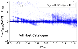
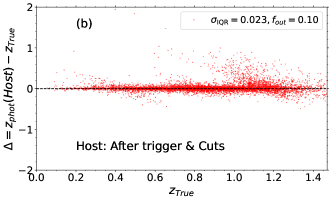
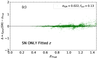
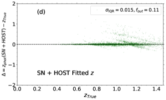
Figure 3: Photo-$z$ residual ($z_{\rm phot}-z_{\rm true}$) vs. $z_{\rm true}$ for (a) full host galaxy catalogue, (b) host galaxy after trigger and selection cuts, (c) SALT2 fitted SN only photo-$z$ without host galaxy prior and (d) Combined SALT2 fitted SN+Host photo-$z$ that is used for the Hubble diagram. Panels (b), (c) and (d) have no $z_{\rm spec}$ events. The $\sigma_{\rm IQR}$ and $f_{\rm out}$ numbers on each panel are computed for $0.4<z_{\rm true}<1.4$.

Table 2: Average depth and time between observations.

	WFD		DDF
Filter	depth	gap	depth	gap
$u$	$23.84$	$10.5$	$25.05$	$5.3$
$g$	$24.80$	$11.9$	$25.52$	$7.3$
$r$	$24.21$	$8.2$	$25.60$	$7.3$
$i$	$23.57$	$8.6$	$25.19$	$7.3$
$z$	$22.65$	$9.0$	$24.79$	$7.3$
$Y$	$21.79$	$11.2$	$23.83$	$7.4$

IV Analysis

The SNIa-cosmology analysis steps are shown in Fig. 4, and described below. This analysis is similar to the recent DC2-SNIa cosmology analysis in Sánchez et al. (2021), except here we include DDF and use photo-$z$ information. The analysis is performed three times, each using the same low-$z$ sample but varying the high-$z$ data:

1. $z_{\rm phot}$: full sample including both spectroscopic and photometric redshifts

2. $z_{\rm spec}$: subset with only accurate spectroscopic redshift from either the host galaxy or SN

3. $z_{\rm cheat}$: full sample forcing $z_{\rm phot}=z_{\rm true}$

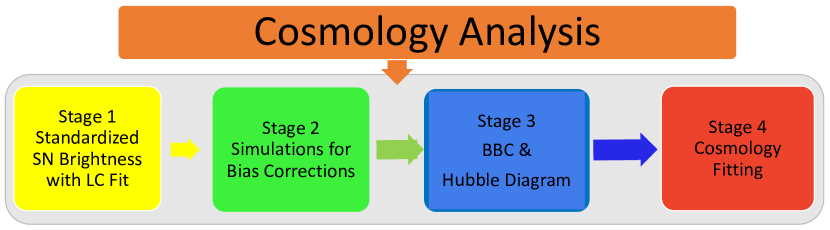
Figure 4: Flowchart showing the cosmology analysis steps.

IV.1 Lightcurve Fitting and Selection Requirements

To standardize the SNIa brightness, we fit each light curve to the SALT2 light curve model (Guy et al., 2010), which determines the time of peak brightness ($t_{0}$), amplitude ($x_{0}$), stretch ($x_{1}$), and color ($c$). Previous cosmology analyses have all used SNe with accurate $z_{\rm spec}$, and thus redshift had always been a fixed parameter in the SALT2 fit. In our analysis, the SALT2 fit uses the methodology in Kessler et al. (2010) in which the redshift is floated as a 5th parameter, which we call “$z_{\rm phot}$”. The host-galaxy photo-$z$ is used as a prior in the SALT2 fit, approximated by a Gaussian with mean and $\sigma$ corresponding to the mean and rms of the photo-$z$ PDF. For the subset with accurate $z_{\rm spec}$, the redshift prior is so precise ($0.0001$) that such fits are essentially equivalent to fixing the redshift in a 4-parameter fit. Note that $z_{\rm phot}$ refers to the fitted redshift for all events, including the $z_{\rm spec}$ subset.

We apply the following selection requirements (cuts) based on analyses using real data:

1. at least three bands with maximum SNR$>4$

2. successful light curve fit

3. $|x_{1}|<3.0$

4. $|c|<0.3$

5. stretch uncertainty $\sigma_{x1}<1.0$

6. time of peak brightness uncertainty $\sigma_{t0}<2.0$ days

7. $P_{\rm fit}>0.05$

8. $0.01<z_{\rm phot}<1.4$

9. valid bias correction (see section §IV.3).

SALT2 light curve fits for several events are shown by the smooth curves in Fig. 1. After selection requirements, the redshift distribution is shown in Fig. 5a for the subset with and without $z_{\rm spec}$.

The $z_{\rm phot}$ residual vs. $z_{\rm true}$ is shown in Fig. 3a for all galaxies in the catalogue, and in Fig. 3b for host galaxies after SN Ia trigger and selection cuts. After selection cuts, SNe associated with host-galaxy photo-$z$ outliers tend to be excluded by the SALT2 fit and $P_{\rm fit}$ cut; the core resolution is reduced by $10\%$, and the outlier fraction is reduced by 20%.

To compare the photo-$z$ precision between the host and SN, we performed SALT2 light curve fits without a host-galaxy photo-$z$ prior to determine the SN-only $z_{\rm phot}$ residuals (Fig. 3c); the SN-only $z_{\rm phot}$ core resolution is slightly $({\sim}1.1)$ better than for the galaxies in Fig. 3a, although the outlier fractions are the same. For the combined SN+host SALT2 fits, Fig. 3d shows $z_{\rm phot}$ residuals vs. $z_{\rm true}$; compared to fitting SN-only, the SN+host $z_{\rm phot}$ resolution is 30% smaller and has $\sim 15\%$ fewer outliers.

To evaluate systematic uncertainties, the SALT2 light curve fits and BBC fit are repeated 7 times, each with a separate variation shown in Table 3. Each variation results in a distance modulus variation, and we compute a systematic covariance matrix (${\rm COV}_{\rm syst}$) using Eq. 6 in (Conley et al., 2011).

We include variations in Galactic extinction, calibration, $z_{\rm spec}$, and host-galaxy $z_{\rm phot}$. We do not include SALT2 modelling and training uncertainties, nor do we include uncertainties on the stretch and color populations.

The galactic extinction uncertainty (Row $2$ in Table 3) is $\sigma_{\rm{MWEBV}}=0.05\cdot\rm{MWEBV}$, and is taken from the Pantheon analysis (Scolnic et al., 2018). The HST calibration uncertainty (Row $3$) is from the DES SNIa-cosmology analysis (Table 4 in Brout et al. (2019)) and is based on Bohlin et al. (2014). The zero point uncertainty (Row 4) is from the LSST science roadmap (section §3.3 in Ivezić et al. (2018)), and is consistent with the Pan-STARRS $3\pi$ internal calibration accuracy (Schlafly et al., 2012; Magnier et al., 2013). The wavelength calibration uncertainty (Row 5) is from the Pantheon analysis in Scolnic et al. (2018).

The spectroscopic redshift uncertainty (Row 6) is from Table 4 in Brout et al. (2019), which is based on low-redshift constraints on local density fluctuations (Calcino and Davis, 2017). For the host-galaxy photo-$z$ bias uncertainty (Row 7), the statistical bias in our PLAsTiCC simulation is well below 0.01 as shown in the lower panel of Fig. 2 in G18. This statistical bias is valid for the galaxy training set, but the bias for the subset of SN Ia host galaxies is likely to be larger. Without a photo-$z$ bias estimate for SN Ia host-galaxies, we make an ad-hoc estimate from the DES weak lensing (WL) cosmology analysis in which Myles et al. (2021) find a statistical $z_{\rm phot}$ bias of ${\sim}0.001$, while their weighted $z_{\rm phot}$ bias is 0.01, an order of magnitude larger. We use their weighted $z_{\rm phot}$ bias of 0.01 as the systematic uncertainty. The uncertainty in the host $z_{\rm phot}$ uncertainty (Row 8) is from the variation in robust standard deviations in the upper panel of Fig 2 in G18.

Table 3: Source of Systematic Uncertainty

Row	Label	Decription	Value
1	StatOnly	no systematic shifts	—
2	MWEBV	shift $E(B-V)$	5%
3	CAL_HST	HST calibration offset	$0.007\times\lambda$
4	CAL_ZP	LSST zero point shift	$5$ mmag
5	CAL_WAVE	LSST Filter shift	$5$ Å
6	zSPEC	shift $z_{\rm spec}$ redshifts	$5\times 10^{-5}$
7	zPHOT	shift $z_{\rm phot}$ redshifts	$0.01$
8	zPHOTERR	scale host $z_{\rm phot}$ uncertainty	$1.2$

IV.2 Simulated Bias Corrections

To implement distance bias corrections in BBC (§IV.3), we generate a large sample of $3.1\times 10^{6}$ events (after cuts, in section III.1) which consists of $2.6\times 10^{6}$ high-$z$ events and $4.4\times 10^{5}$ low-$z$ events. The bias correction is applied independently for high-$z$ and low-$z$, and thus the relative number of events in each sub-sample need not match the data. The simulation procedure is identical to that used for the simulated data, except for $\alpha$ and $\beta$. While fixed values are used for the data sample, a $2\times 2$ $\alpha,\beta$ grid is used for the “biasCor” simulation to enable interpolation in BBC.

IV.3 BEAMS with Bias Corrections (BBC)

BBC reads the SALT2 fitted parameters (high-$z$ and low-$z$) from the data and biasCor simulation, and produces a bias-corrected Hubble diagram, both unbinned and in redshift bins. For each event, the measured distance modulus is based on Tripp (1998),

$$\mu=m_{B}+\alpha x_{1}-\beta c+M_{0}+\Delta\mu_{\rm bias}~{},$$ (4)

where $m_{B}\equiv-2.5\log_{10}(x_{0})$, $\{\alpha,\beta,M_{0}\}$ are global nuisance parameters, and $\Delta\mu_{\rm bias}=\mu-\mu_{\rm true}$ is determined from the biasCor simulation in a 5-dimensional space of $\{z,x_{1},c,\alpha,\beta\}$. A valid bias correction is required for each event, resulting in a few percent loss. The distance uncertainty ($\sigma_{\mu}$) is computed from Eq. 3 of KS17. Since there is no contamination from non-SNIa, all SN Ia classification probabilities are set to 1 and we do not use the BEAMS formalism.

There are two subtle issues concerning the use of $z_{\rm phot}$ and its uncertainty $\sigma_{z}$. First, the calculated distance error from $\sigma_{z}$ ($\sigma_{\mu}^{z}$ in Eq. 3 of KS17) is an overestimate because it does not account for the correlated color error that reduces the distance error. By floating $z_{\rm phot}$ in the SALT2 fit, redshift correlations propagate to the other SALT2 parameter uncertainties, and therefore we set $\sigma_{\mu}^{z}=0$. The second issue concerns the $\mu_{\mathrm{{bias}}}$ computation, where $\mu_{\rm true}$ is computed at SALT2-fitted $z_{\rm phot}$ rather than the true redshift.

To avoid a dependence on cosmological parameters, the BBC fit is performed in 14 logarithmically-spaced redshift bins. The fitted parameters include the global nuisance parameters ($\alpha,\beta,M_{0}$) and bias-corrected distances in 14 redshift bins. The unbinned Hubble diagram is obtained from Eq. 4 using the fitted parameters.

If the same selection requirements are applied to each systematic variation for computing ${\rm COV}_{\rm syst}$, small fluctuations in the fitted SALT2 parameters and redshift result in slightly different samples, and these differences introduce statistical noise in ${\rm COV}_{\rm syst}$. We avoid this covariance noise by defining a baseline sample for events passing cuts without systematic variations, and use this same baseline sample for all systematic variations. For example, if an event has fitted SALT2 color parameter $c=0.299$, and migrates to $c=0.3001$ for a calibration systematic, this event is preserved without applying cuts that require $|c|<0.3$.

To avoid sample differences from the valid bias-correction requirement, the BBC fit is run twice in which the second fit only includes events that have a valid bias correction in all systematic variations. Finally, for redshift systematics that result in migration to another redshift bin, the original (no syst) redshift bin is preserved for the BBC fit.

IV.4 Cosmology Fitting and Figure of Merit

For cosmology fitting, we use a fast minimization program that approximates a CMB prior using the $R$-shift parameter (e.g., see Eq. 69 in Komatsu et al. (2009)) computed from the same cosmological parameters that were used to generated the SNe Ia. The $R$-uncertainty is $\sigma_{R}=0.006$, tuned to have the same constraining power as Planck Collaboration et al. (2020). We fit with $w$CDM and $w_{0}w_{a}$CDM models, where $w=[w_{0}+w_{a}(1-a)]$. The statistical+systematics covariance matrix is used. We fit both binned and unbinned Hubble diagrams.

For the $w_{0}w_{a}$CDM model, the FoM is computed based on the dark energy task force (DETF) definition in Albrecht et al. (2006),

$$\text{FoM}\simeq\frac{1}{\sigma(w_{a})\sigma(w_{0})\sqrt{1-\rho^{2}}}~{},$$ (5)

where $\rho$ is the reduced covariance between $w_{0}$ and $w_{a}$.

V Results

For one of the 25 statistically independent samples, we show the $z_{\rm spec}$ and $z_{\rm phot}$ Hubble diagram produced by the BBC fit, both binned and unbinned, in Fig. 6. The Hubble residuals with respect to the true cosmology, $\Delta\mu=\mu-\mu_{\rm true}$, are consistent with zero and do not show a redshift-dependent slope.

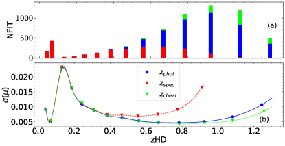
Figure 5: Number of events (top) and BBC-fitted distance uncertainty (bottom) per redshift bin. The three sets of overlaid plots correspond to $z_{\rm spec}$ (red), $z_{\rm phot}$ (blue), and $z_{\rm cheat}$ (green).

The BBC-fitted nuisance parameters are shown in Table 4 for the three analyses: $z_{\rm spec}$, $z_{\rm phot}$, $z_{\rm cheat}$. Averaging over the 25 samples, $\alpha$ and $\beta$ agree well with the simulated inputs. There is no true $\sigma_{\rm int}$ for comparison, but we note that the $\sigma_{\rm int}$ values agree well among the three analyses.

Table 4: Bias for BBC Fitted Nuisance Parameters

Sample	$\alpha-\alpha_{\rm true}$		$\beta-\beta_{\rm true}$		$\sigma_{\rm int}$
$z_{\rm spec}$	$0.00015\pm 0.00158$		$-0.00011\pm 0.02035$		$0.095$
$z_{\rm phot}$	$0.00033\pm 0.00121$		$-0.00017\pm 0.01624$		$0.096$
$z_{\rm cheat}$	$0.00049\pm 0.00112$		$0.00125\pm 0.01549$		$0.095$

Next, we compare the BBC fitted distance uncertainties ($\sigma_{\mu}$) in redshift bins (Fig. 5b) The $z_{\rm spec}$ and $z_{\rm phot}$ uncertainties are similar for $z<0.5$, and at higher redshifts the $z_{\rm phot}$ uncertainty is significantly smaller than for $z_{\rm spec}$. In addition to smaller distance uncertainties, the $z_{\rm phot}$ redshift range extends ${\sim}0.3$ beyond that of the $z_{\rm spec}$ range.

At high redshift, the $z_{\rm cheat}$ analysis shows little improvement over the $z_{\rm phot}$ analysis. Defining an effective distance uncertainty per event in each redshift bin as $\overline{\sigma_{\mu}}_{z}={\sigma_{\mu}}_{z}\times\sqrt{N_{z}}$, where $N_{z}$ is the number of events in the redshift bin, the $\overline{\sigma_{\mu}}_{z}$ values for $z_{\rm cheat}$ and $z_{\rm phot}$ are the same to within a few percent. There are fewer $z_{\rm phot}$ events (compared to $z_{\rm cheat}$) because of selection cuts and unstable results between multiple light curve fit iterations.

For the cosmology fitting, we fit the binned distances from the BBC fit and also performed unbinned fits to reduce the systematic uncertainty as described in Brout et al. (2021). While the unbinned cosmology fits result in smaller uncertainties, we find a significant bias that is driven by the calibration systematics. We have not found an explanation of this bias, and therefore we present results only for binned distances.

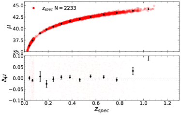
(a)

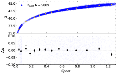
(b)

Figure 6: For one of the 25 statistically independent samples, redshift binned (solid black circles) and unbinned Hubble diagram from BBC fit, for $z_{\rm spec}$ (top) and $z_{\rm phot}$ (bottom) samples. Each lower panel shows Hubble residual $\Delta\mu$ with respect to the true cosmology: the error bar shows the rms in each BBC redshift bin (same redshift bins as in Fig. 5).

For the subsections below, we define $w$-bias to be $w-w_{\rm true}$ where $w$ is from the $w$CDM  cosmology fit. A similar definition is used for $w_{0}$ and $w_{a}$ for the $w_{0}w_{a}$CDM model.

V.1 $w$CDMResults

For the $w$CDM cosmology fits, Table 5 shows the average $w$-bias and average uncertainty among the $25$ samples. The average $w$-bias is consistent with zero for both the $z_{\rm spec}$ and $z_{\rm phot}$ samples, and also with and without systematic uncertainties. The $w$-bias precision is ${\sim}0.002$. The average $w$-uncertainty ($\langle\sigma_{w}\rangle$) for the $z_{\rm phot}$ sample is $0.023$, with systematics, and is only slightly improved compared to $\langle\sigma_{w}\rangle=$$0.025$ for the $z_{\rm spec}$ sample. The additional sensitivity from the host-galaxy $z_{\rm phot}$ sample is small because the increased statistics are at higher redshifts where the dark energy density fraction is much smaller compared to lower redshifts where the sample is dominated by spectroscopic redshifts.

Table 5: Summary of $w$CDM Cosmology Fits

redshift
source	Systematics	$\langle w$-bias$\rangle$	$\langle\sigma_{w}\rangle$
$z_{\rm spec}$	Stat only	$-0.0008\pm 0.0020$	$0.020$
	Stat$+$Syst	$-0.0027\pm 0.0025$	$0.025$
$z_{\rm phot}$	Stat only	$-0.0003\pm 0.0017$	$0.020$
	Stat$+$Syst	$-0.0009\pm 0.0018$	$0.023$

V.2 $w_{0}w_{a}$CDMResults

For the $w_{0}w_{a}$CDM model, the average bias, uncertainty, and FoM are shown in Table 6. While there was little improvement using the $z_{\rm phot}$ sample with the $w$CDM model, the $w_{0}w_{a}$CDM  improvement is much more significant because higher redshift events, which are enhanced by the $z_{\rm phot}$ sample, are more sensitive to evolving dark energy ($w_{a}$). With systematics, ${\langle}{\rm FoM}{\rangle}=$$95$ for the $z_{\rm spec}$ sample and ${\langle}{\rm FoM}{\rangle}=$$145$ for the $z_{\rm phot}$ sample. The $w_{0}$-$w_{a}$ constraining power is shown in Fig. 7 for a single simulated data sample.

Table 6: Summary of $w_{0}w_{a}$CDM Cosmology Fits

$z$
source	Syst	$\langle{w_{0}}$-bias$\rangle$	$\langle{w_{a}}$-bias$\rangle$	$\langle\sigma_{w_{0}}\rangle$	$\langle\sigma_{w_{a}}\rangle$	${\langle}{\rm FoM}{\rangle}$
$z_{\rm spec}$	Stat only	$0.0083\pm 0.0143$	$-0.0658\pm 0.0674$	$0.076$	$0.353$	$136$
	Stat$+$Syst	$0.0067\pm$$0.0140$	$-0.0683\pm$$0.0662$	$0.092$	$0.418$	$95$
$z_{\rm phot}$	Stat only	$0.0029\pm 0.0082$	$-0.0228\pm 0.0342$	$0.048$	$0.211$	$237$
	Stat$+$Syst	$0.0011\pm$$0.0091$	$-0.0202\pm$$0.0363$	$0.071$	$0.294$	$145$

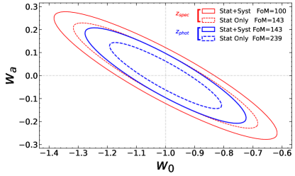
Figure 7: $w_{0}$-$w_{a}$$2\sigma$ $(95\%$ confidence$)$ contours and FoM for a single SNIa data sample combined with CMB prior, and shifted to be centered at $w_{0},w_{a}=-1,0$. Contours for $z_{\rm phot}$ ($z_{\rm spec}$) are shown in blue (red). Solid (dashed) contours show stat+syst (stat-only).

The average bias is consistent with zero for both $w_{0}$ and $w_{a}$. For the $z_{\rm spec}$ sample, the bias precision is ${\sim}0.015$ and ${\sim}0.07$ for $w_{0}$ and $w_{a}$, respectively. For the $z_{\rm phot}$ sample, the bias precision is improved to ${\sim}0.009$ and ${\sim}0.04$. The $w_{0}$-$w_{a}$ average bias is shown in Fig. 8, and compared to the the $w_{0}$-$w_{a}$ contours (statistical+systematic) for a single sample.

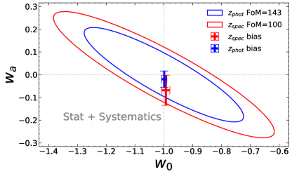
Figure 8: $w_{0}$-$w_{a}$ $2\sigma$ contours and FoM for $z_{\rm phot}$ (blue) and $z_{\rm spec}$ (red) for a single data sample. The crosses show the $\pm 1\sigma$ bias from averaging results over the 25 simulated data samples.

For the $z_{\rm phot}$ sample, the figure-of-merit averaged over 25 samples is ${\langle}{\rm FoM}{\rangle}=$$237$ with only statistical uncertainties, and drops to ${\langle}{\rm FoM}{\rangle}=$$145$  when systematic uncertainties are included. Since there are many systematics contributing to the decrease in ${\langle}{\rm FoM}{\rangle}$, we quantify the impact of each systematic “$i$” by recomputing the covariance matrix separately for each systematic (${\rm COV}_{{\rm syst},i}$), and repeating the cosmology fit for each ${\rm COV}_{{\rm syst},i}$. We finally compute the FoM ratios

$${\cal R}_{{\rm FoM},i}={\rm FoM}_{{\rm syst},i}/{\rm FoM}_{\rm stat}~{},$$ (6)

where ${\rm FoM}_{{\rm syst},i}$ is the FoM from including only systematic $i$, and ${\rm FoM}_{\rm stat}$ is the FoM without systematic uncertainties. Note that ${\cal R}_{{\rm FoM},i}\leq 1$. Table 7 shows the ${\cal R}_{{\rm FoM},i}$, and the FoM degradation is dominated by the calibration systematics.

V.3 Discussion of photo-$z$ Systematics

The 0.01 photo-$z$ shift systematic has a small (2%) effect on FoM for three reasons. First, the combined SN+host light curve fit results in an average fitted redshift error of ${\sim}0.004$, or about half the host photo-$z$ error. Second, this photo-$z$ systematic does not affect $z_{\rm spec}$ events which dominate the lower redshift region below about 0.5 (Fig. 5a), and this $z_{\rm spec}$ region is most sensitive to redshift errors. The final reason is that the fitted $z_{\rm phot}$ and SALT2 color are anti-correlated and thus a larger (smaller) $z_{\rm phot}$ results in bluer (redder) color, and this change in color self-corrects the distance error as illustrated in Fig. 9.

To describe this distance self-correction, we first define $\Delta z_{\rm syst-z}$ as the difference between SALT2-fitted $z_{\rm phot}$ with 0.01 host-galaxy photo-$z$ shift and nominal photo-$z$, and similarly define $\Delta\mu_{\rm syst-z}$ as the distance difference from Eq. 4. Fig 9a shows $\Delta\mu_{\rm syst-z}$ vs $\Delta z_{\rm syst-z}$ and a linear fit for the slope, $d\mu/dz$, in one of five $z_{\rm true}$ bins. Fig 9b shows the measured $d\mu/dz$ slope in five $z_{\rm true}$ bins (black circles) along with the $\Lambda{\rm CDM}$ theory curve in red. In the ideal limit where the measured $d\mu/dz$ exactly equal theory $d\mu/dz$, the distance self-correction is perfect and results in no systematic uncertainty. Here the measured $d\mu/dz$ are close to the theory curve, and thus the distance error is mostly corrected.

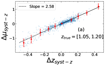
(a)

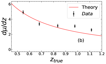
(b)

Figure 9: (a) $\Delta\mu_{\rm syst-z}$ vs. $\Delta z_{\rm syst-z}$ for 0.01 systematic shift in host-galaxy photo-$z$, and linear fit with slope $d\mu/dz$, (b) fitted slope $d\mu/dz$ in five $z_{\rm true}$ bins (black circles with error bars), and $\Lambda{\rm CDM}$ theory curve in red.

Table 7: FoM-Ratio ${\cal R}_{{\rm FoM},i}$ for Each Systematic ($w_{0}w_{a}$CDM model)

	${\cal R}_{{\rm FoM},i}$
Systematic(s)	$z_{\rm phot}$   $z_{\rm spec}$
None (stat only)	$1.00\ \ 1.00\ \$
MWEBV	$0.99\ \ 1.00\ \$
ZERRSCALE	$0.99\ \ 1.00\ \$
zSHIFT	$0.98\ \ 0.99\ \$
Photo-z Shift	$0.98\ \ 0.99\ \$
CAL$\_$WAVE	$0.90\ \ 0.94\ \$
CAL$\_Z_{p}$	$0.71\ \ 0.75\ \$
CAL	$0.64\ \ 0.71\ \$
Stat $+$ All Syst	$0.61\ \ 0.70\ \$

To gain further insight into the photo-$z$ sensitivity, we first consider a naive systematic of shifting the fitted $z_{\rm phot}$ by 0.01 after the light curve fit, for the subset without a $z_{\rm spec}$. In this test, the compensating $d\mu/dz$ points in Fig. 9 are forced to be zero, and there is no systematic reduction from a combined SN+host fit. Fitting the $w_{0}w_{a}$CDM model without ${\rm COV}_{\rm syst}$, the $w_{0}$ and $w_{a}$ biases are 0.03 and 0.15, respectively. Next we consider the realistic case of shifting the host photo-$z$ before the SALT2 light curve fit; the corresponding $w_{0}$ and $w_{a}$ biases are 0.001 and 0.003, more than an order of magnitude smaller than the naive systematic. While we have included an explicit host-galaxy photo-$z$ systematic, there is no explicit analogue for the SN. The SN photo-$z$ systematic is accounted for by the calibration and Galactic extinction contributions to the systematic uncertainty budget in Table 3, but it is difficult to untangle the impact of these systematics on distance and photo-$z$.

VI Conclusions

In this work we presented cosmological dark energy constraints for simulated PLAsTiCC-SN Ia data, and we continued the development of publicly available codes from SNANA and Pippinto analyse the the data with a host galaxy photo-$z$ prior. For the $w_{0}w_{a}$CDM model, the dark energy figure of merit is FoM${\sim}$$237$ with only statistical uncertainties, and drops to ${\sim}$$145$ with systematic uncertainties (Fig. 7). This $z_{\rm phot}$ FoM is 50% larger than the FoM obtained from the $z_{\rm spec}$ subset that has a spectroscopic redshift from the host or SN. Averaging 25 independent data samples, the average bias on $w_{0}$ and $w_{a}$ is consistent with zero.

The systematic uncertainty from the host-galaxy photo-$z$ results in only a 2% reduction in the FoM. This small impact is due to i) nearly complete $z_{\rm spec}$ at lower redshifts, ii) smaller $z_{\rm phot}$ bias from combining the SN and host, and iii) anti-correlations between redshift and color that greatly reduce the distance error. While good $z_{\rm spec}$ coverage is feasible for the DDF, the WFD will likely have less $z_{\rm spec}$ coverage and using host-galaxy photo-$z$’s at lower redshifts may increase the systematic uncertainty compared to this DDF analysis.

Simulated projections tend to be overly optimistic before a survey begins, particularly for the depth and average PSF. However, there are three key factors that are likely to improve future results: 1) here we simulated only 30% of the 10-year baseline survey, 2) we used a CMB prior with constraining power to match Planck Collaboration et al. (2020), and did not assume improved CMB constraints during the LSST era, 3) we did not include the ${\sim}50$% FoM-increase from fitting an unbinned Hubble diagram; this improvement awaits resolving the large $w_{0}$-$w_{a}$ bias associated with unbinned results.

Most SNIa-cosmology analyses over the past decade have used redshift binned Hubble diagrams. These analyses include, JLA (Betoule et al., 2014), Pantheon (Scolnic et al., 2018), PS1 single instrument (Jones et al., 2018) and DES (Abbott et al., 2019). The recent demonstration of smaller uncertainties with an unbinned Hubble diagram has not been rigorously tested until our analysis that shows biased cosmology parameters. We therefore encourage community effort to resolve this issue.

The next major effort is to develop the cosmology analysis for samples that include non-SNIa contamination, host galaxy mis-association, and a more complete list of systematic uncertainties that includes host galaxy photo-$z$ model and intrinsic scatter of the SN brightness. Cosmology analyses using photometric classification and spectroscopic redshifts have been well developed on real data from PS1 (Jones et al., 2018) and from DES (Vincenzi et al., 2022). Here we have developed and demonstrated a complimentary analysis using photometric redshifts and a spectroscopically confirmed sample.

References

- Perlmutter et al. (1999) S. Perlmutter, G. Aldering, G. Goldhaber, R. A. Knop, P. Nugent, et al., Astrophys. J. 517, 565 (1999), eprint astro-ph/9812133.
- Riess et al. (1998) A. G. Riess, A. V. Filippenko, P. Challis, A. Clocchiatti, A. Diercks, et al., Astron. J 116, 1009 (1998), eprint astro-ph/9805201.
- Linder (2003) E. V. Linder, Phys. Rev. Lett. 90, 091301 (2003), eprint astro-ph/0208512.
- Chevallier and Polarski (2001) M. Chevallier and D. Polarski, International Journal of Modern Physics D 10, 213 (2001), eprint gr-qc/0009008.
- Betoule et al. (2014) M. Betoule et al., Astron. Astrophys. 568, A22 (2014), eprint 1401.4064.
- Scolnic et al. (2018) D. M. Scolnic, D. O. Jones, A. Rest, Y. C. Pan, R. Chornock, R. J. Foley, M. E. Huber, R. Kessler, G. Narayan, A. G. Riess, et al., Astrophys. J. 859, 101 (2018), eprint 1710.00845.
- Abbott et al. (2019) T. M. C. Abbott, S. Allam, P. Andersen, C. Angus, J. Asorey, et al. (DES Collaboration), Astrophys. J. Lett. 872, L30 (2019), eprint 1811.02374.
- Brout et al. (2022) D. Brout et al. (2022), eprint 2202.04077.
- Lochner et al. (2016) M. Lochner et al., Astrophys. J. Suppl. 225, 31 (2016), eprint 1603.00882.
- Möller and de Boissière (2020) A. Möller and T. de Boissière, Mon. Not. Roy. Astron. Soc. 491, 4277 (2020), eprint 1901.06384.
- Kessler et al. (2010) R. Kessler, D. Cinabro, B. Bassett, B. Dilday, J. A. Frieman, et al., Astrophys. J. 717, 40 (2010), eprint 1001.0738.
- Palanque-Delabrouille et al. (2010) N. Palanque-Delabrouille, V. Ruhlmann-Kleider, S. Pascal, J. Rich, J. Guy, G. Bazin, P. Astier, C. Balland, S. Basa, R. G. Carlberg, et al., Astron. Astrophys. 514, A63 (2010), eprint 0911.1629.
- Roberts et al. (2017) E. Roberts, M. Lochner, J. Fonseca, B. A. Bassett, P.-Y. Lablanche, and S. Agarwal, J. Cosmol. Astropart. Phys. 10, 036 (2017), eprint 1704.07830.
- Kunz et al. (2007) M. Kunz, B. A. Bassett, and R. A. Hlozek, Phys. Rev. D 75, 103508 (2007), eprint astro-ph/0611004.
- Hlozek et al. (2012) R. Hlozek, M. Kunz, B. Bassett, M. Smith, J. Newling, et al., Astrophys. J. 752, 79 (2012), eprint 1111.5328.
- Jones et al. (2018) D. O. Jones, D. M. Scolnic, A. G. Riess, A. Rest, R. Kirshner, et al., Astrophys. J. 857, 51 (2018), eprint 1710.00846.
- Kessler and Scolnic (2017) R. Kessler and D. Scolnic, Astrophys. J. 836, 56 (2017), eprint 1610.04677.
- Vincenzi et al. (2022) M. Vincenzi, M. Sullivan, A. Möller, P. Armstrong, B. A. Bassett, D. Brout, D. Carollo, A. Carr, T. M. Davis, C. Frohmaier, et al., "Mon. Not. Roy. Astron. Soc." (2022), eprint 2111.10382.
- Guy et al. (2007) J. Guy, P. Astier, S. Baumont, D. Hardin, R. Pain, N. Regnault, S. Basa, R. G. Carlberg, A. Conley, S. Fabbro, et al., Astron. Astrophys. 466, 11 (2007), eprint astro-ph/0701828.
- Dai et al. (2018) M. Dai et al., Mon. Not. Roy. Astron. Soc. 477, 4142 (2018), eprint 1701.05689.
- Chen et al. (2022) R. Chen, D. Scolnic, E. Rozo, E. S. Rykoff, B. Popovic, R. Kessler, M. Vincenzi, T. M. Davis, P. Armstrong, D. Brout, et al., arXiv e-prints arXiv:2202.10480 (2022), eprint 2202.10480.
- Linder and Mitra (2019) E. V. Linder and A. Mitra, Phys. Rev. D 100, 043542 (2019), eprint 1907.00985.
- Mitra and Linder (2021) A. Mitra and E. V. Linder, Phys. Rev. D 103, 023524 (2021), eprint 2011.08206.
- Kessler et al. (2019a) R. Kessler, G. Narayan, A. Avelino, E. Bachelet, R. Biswas, P. J. Brown, D. F. Chernoff, A. J. Connolly, M. Dai, S. Daniel, et al., Publ. Astron. Soc. Pac. 131, 094501 (2019a), eprint 1903.11756.
- Kessler et al. (2009) R. Kessler, J. P. Bernstein, D. Cinabro, B. Dilday, J. A. Frieman, S. Jha, S. Kuhlmann, G. Miknaitis, M. Sako, M. Taylor, et al., "Publ. Astron. Soc. Pac." 121, 1028 (2009), eprint 0908.4280.
- Hinton and Brout (2020) S. Hinton and D. Brout, The Journal of Open Source Software 5, 2122 (2020).
- Cahn (2009) R. N. Cahn, Dark Energy Task Force (World Scientific, 2009), pp. 685–695.
- Ivezić et al. (2019) v. Ivezić et al. (LSST), Astrophys. J. 873, 111 (2019), eprint 0805.2366.
- LSST Dark Energy Science Collaboration et al.(2021)LSST Dark Energy Science Collaboration (LSST DESC), Abolfathi, Alonso, Armstrong, Aubourg, Awan, Babuji, Bauer, Bean, Beckett et al. (LSST DESC) LSST Dark Energy Science Collaboration (LSST DESC), B. Abolfathi, D. Alonso, R. Armstrong, É. Aubourg, H. Awan, Y. N. Babuji, F. E. Bauer, R. Bean, G. Beckett, et al., Astrophys. J., Suppl. Ser. 253, 31 (2021), eprint 2010.05926.
- Sánchez et al. (2021) B. Sánchez, R. Kessler, D. Scolnic, B. Armstrong, R. Biswas, J. Bogart, J. Chiang, J. Cohen-Tanugi, D. Fouchez, P. Gris, et al., arXiv e-prints arXiv:2111.06858 (2021), eprint 2111.06858.
- Lokken et al. (2022) M. Lokken et al. (LSST Dark Energy Science) (2022), eprint 2206.02815.
- Alard and Lupton (1998) C. Alard and R. H. Lupton, Astrophys. J. 503, 325 (1998), eprint astro-ph/9712287.
- Fukugita et al. (1996) M. Fukugita, T. Ichikawa, J. E. Gunn, M. Doi, K. Shimasaku, and D. P. Schneider, Astron. J 111, 1748 (1996).
- Hložek et al. (2020) R. Hložek, K. A. Ponder, A. I. Malz, M. Dai, G. Narayan, E. E. O. Ishida, J. Allam, T., A. Bahmanyar, R. Biswas, L. Galbany, et al., arXiv e-prints arXiv:2012.12392 (2020), eprint 2012.12392.
- Graham et al. (2018) M. L. Graham, A. J. Connolly, Ž. Ivezić, S. J. Schmidt, R. L. Jones, M. Jurić, S. F. Daniel, and P. Yoachim, Astron. J. 155, 1 (2018), eprint 1706.09507.
- Kessler et al. (2019b) R. Kessler, D. Brout, C. B. D’Andrea, T. M. Davis, S. R. Hinton, A. G. Kim, J. Lasker, C. Lidman, E. Macaulay, A. Möller, et al., Mon. Not. Roy. Astron. Soc. 485, 1171 (2019b), eprint 1811.02379.
- Scolnic and Kessler (2016) D. Scolnic and R. Kessler, Astrophys. J. Lett. 822, L35 (2016), eprint 1603.01559.
- Pierel et al. (2018) J. D. R. Pierel, S. Rodney, A. Avelino, F. Bianco, A. V. Filippenko, R. J. Foley, A. Friedman, M. Hicken, R. Hounsell, S. W. Jha, et al., Publ. Astron. Soc. Pac. 130, 114504 (2018), eprint 1808.02534.
- Schlafly and Finkbeiner (2011) E. F. Schlafly and D. P. Finkbeiner, Astrophys. J. 737, 103 (2011), eprint 1012.4804.
- Delgado et al. (2014) F. Delgado, A. Saha, S. Chandrasekharan, K. Cook, C. Petry, and S. Ridgway, in Modeling, Systems Engineering, and Project Management for Astronomy VI, edited by G. Z. Angeli and P. Dierickx (2014), vol. 9150 of Society of Photo-Optical Instrumentation Engineers, p. 915015.
- OpS (2016) Observatory Operations: Strategies, Processes, and Systems VI, vol. 9910 of Society of Photo-Optical Instrumentation Engineers (2016).
- Reuter et al. (2016) M. A. Reuter et al., in Modeling, Systems Engineering, and Project Management for Astronomy VI, edited by G. Z. Angeli and P. Dierickx (2016), vol. 9911 of Society of Photo-Optical Instrumentation Engineers (SPIE), p. 991125.
- de Jong et al. (2019) R. S. de Jong, O. Agertz, A. A. Berbel, J. Aird, D. A. Alexander, et al., The Messenger 175, 3 (2019), eprint 1903.02464.
- Dilday et al. (2008) B. Dilday, R. Kessler, J. A. Frieman, J. Holtzman, J. Marriner, G. Miknaitis, R. C. Nichol, R. Romani, M. Sako, B. Bassett, et al., Astrophys. J. 682, 262 (2008), eprint 0801.3297.
- Hounsell et al. (2018) R. Hounsell, D. Scolnic, R. J. Foley, R. Kessler, V. Miranda, A. Avelino, R. C. Bohlin, A. V. Filippenko, J. Frieman, S. W. Jha, et al., Astrophys. J. 867, 23 (2018), eprint 1702.01747.
- Guy et al. (2010) J. Guy et al., Astron. Astrophys. 523, A7 (2010), eprint 1010.4743.
- Conley et al. (2011) A. Conley, J. Guy, M. Sullivan, N. Regnault, P. Astier, C. Balland, S. Basa, R. G. Carlberg, D. Fouchez, D. Hardin, et al., Astrophys. J. Lett. Suppl. 192, 1 (2011), eprint 1104.1443.
- Brout et al. (2019) D. Brout et al. (DES), Astrophys. J. 874, 150 (2019), eprint 1811.02377.
- Bohlin et al. (2014) R. C. Bohlin, K. D. Gordon, and P. E. Tremblay, Publ. Astron. Soc. Pac. 126, 711 (2014), eprint 1406.1707.
- Ivezić et al. (2018) Ž. Ivezić et al. (2018).
- Schlafly et al. (2012) E. F. Schlafly, D. P. Finkbeiner, M. Jurić, E. A. Magnier, W. S. Burgett, K. C. Chambers, T. Grav, K. W. Hodapp, N. Kaiser, R. P. Kudritzki, et al., Astrophys. J. 756, 158 (2012), eprint 1201.2208.
- Magnier et al. (2013) E. A. Magnier, E. Schlafly, D. Finkbeiner, M. Juric, J. L. Tonry, W. S. Burgett, K. C. Chambers, H. A. Flewelling, N. Kaiser, R. P. Kudritzki, et al., Astrophys. J. Lett. Suppl. 205, 20 (2013), eprint 1303.3634.
- Calcino and Davis (2017) J. Calcino and T. Davis, J. Cosmol. Astropart. Phys. 2017, 038 (2017), eprint 1610.07695.
- Myles et al. (2021) J. Myles, A. Alarcon, A. Amon, C. Sánchez, S. Everett, J. DeRose, J. McCullough, D. Gruen, G. M. Bernstein, M. A. Troxel, et al., Mon. Not. Roy. Astron. Soc. 505, 4249 (2021), eprint 2012.08566.
- Tripp (1998) R. Tripp, Astron. Astrophys. 331, 815 (1998).
- Komatsu et al. (2009) E. Komatsu et al., Astrophys. J.s 180, 330 (2009), eprint 0803.0547.
- Planck Collaboration et al. (2020) Planck Collaboration, N. Aghanim, Y. Akrami, M. Ashdown, J. Aumont, C. Baccigalupi, et al. (Planck), Astron. Astrophys. 641, A6 (2020), [Erratum: Astron.Astrophys. 652, C4 (2021)], eprint 1807.06209.
- Albrecht et al. (2006) A. Albrecht et al., arXiv e-prints (2006), eprint astro-ph/0609591.
- Brout et al. (2021) D. Brout, S. R. Hinton, and D. Scolnic, Astrophysical Journal, Letters 912, L26 (2021), eprint 2012.05900.