Estimation of High-Dimensional Markov-Switching VAR Models with an Approximate EM Algorithm

Abstract

Regime shifts in high-dimensional time series arise naturally in many applications, from neuroimaging to finance. This problem has received considerable attention in low-dimensional settings, with both Bayesian and frequentist methods used extensively for parameter estimation. The EM algorithm is a particularly popular strategy for parameter estimation in low-dimensional settings, although the statistical properties of the resulting estimates have not been well understood. Furthermore, its extension to high-dimensional time series has proved challenging. To overcome these challenges, in this paper we propose an approximate EM algorithm for Markov-switching VAR models that leads to efficient computation and also facilitates the investigation of asymptotic properties of the resulting parameter estimates. We establish the consistency of the proposed EM algorithm in high dimensions and investigate its performance via simulation studies.

Keywords: High-Dimensional Time Series; Penalized Estimation; $\beta$-Mixing.

1 Introduction

The presence of regime shifts is an important feature for many time series arising from various applications; that is, the time series may exhibit changing behavior over time. While some of these regime shifts are attributable to certain deterministic structural changes, in many cases the dynamics of the observed time series is governed by an exogenous stochastic process that determines the regime. For example, the behavior of key macroeconomic indicators may depend on the phase of the business cycle, for example, recession versus expansion (Hamilton, 1989; Artis et al., 2004); the relationship between stock market return and exchange rate may vary between high- and low-volatility regimes (Chkili and Nguyen, 2014); in neuroimaging studies, the connectivity between different brain regions may change over time according to the brain’s underlying states (Fiecas et al., 2021). As in these examples, the exogenous process that determines the regime is oftentimes latent or not directly observable. This relates naturally to the notion of state-space models (Koller and Friedman, 2009).

A prominent example of such a state-space model is the hidden Markov model (HMM) (see, for example, Rabiner, 1989). In an HMM, the observations over time are conditionally independent given a latent process that determines the state, and the state process is assumed to be a Markov chain. Markov-switching vector autoregression (VAR) (Krolzig, 2013) can be regarded as a generalization of the HMM model that allows for autoregression. In a Markov-switching VAR model, the dynamics of the observed time series takes a VAR form, but the autoregressive parameters depend on the state of a latent finite-state Markov chain. As such, Markov-switching VAR models have found widespread applications, in areas such as macroeconomics (Krolzig, 2013, and the references therein) and ecology (Solari and Van Gelder, 2011). Estimation of the autoregressive parameters and the transition of the latent regime process is often of central interest in these applications.

Bayesian approaches have been developed (Fox et al., 2010) and applied for parameter estimation in Markov-switching VARs using various prior distributions for the model parameters (Billio et al., 2016; Droumaguet et al., 2017). Alternatively, the expectation-maximization (EM) algorithm (Dempster et al., 1977) provides a general approach for computing the maximum likelihood estimator in latent variable and incomplete data problems. Application of the EM algorithm in Markov-switching VAR models dates back to Lindgren (1978) and Hamilton (1989), and the method has gained great popularity since then. However, to the best of our knowledge, the theoretical properties of the estimate obtained using the EM algorithm in Markov-switching VAR problems have not been rigorously investigated, even in low-dimensional settings.

Earlier theoretical studies of the EM algorithm established its convergence to the unique global optimum under unimodality of the likelihood function (Wu, 1983), but only to some local optimum in general cases where the likelihood function is multi-modal (for example, McLachlan and Krishnan, 2007). Recent work by Balakrishnan et al. (2017) establishes statistical guarantees for the EM estimate in low-dimensional settings, when the algorithm is initialized within a local region around the true parameter. Under certain conditions, the authors show geometric convergence to an EM fixed point that is within statistical precision of the true parameter. Wang et al. (2014) extends the EM algorithm to high-dimensional settings (where the number of parameters is larger than sample size), by introducing truncation in the M-step. In contrast, Yi and Caramanis (2015) develops a regularized EM algorithm for high-dimensional problems that incorporates regularization in the M-step. It also establish general statistical guarantee for the resulting parameter estimate. Regularized EM algorithms are also studied in specific contexts, including high-dimensional mixture regression (Städler et al., 2010) and graphical models (Hao et al., 2017). However, all of these works consider a sample of independent and identically distributed observations.

Regularized EM algorithms have been considered in the context of Markov-switching VAR models in Monbet and Ailliot (2017) and Maung (2021), allowing the number of parameters to diverge; however, these works did not analyze the statistical properties of the EM estimate, which is challenging in time series settings. A major source of complication in this setting arises from the dependence of the conditional expectation in the E-step on observations in all the past time points, due to the unobserved latent variables. In this work, we develop a regularized EM algorithm for parameter estimation in high-dimensional Markov-switching VAR models, and rigorously establish its performance guarantee. To deal with the temporal dependence among observations, we introduce an approximate E-step, in which we compute approximate conditional expectations. In addition to facilitating theoretical analysis, this approximation also leads to improved computation. To establish the consistency of the proposed algorithm, we apply novel probabilistic tools for ergodic time series.

The rest of this paper is organized as follows. In Section 2, we introduce Markov-switching VAR models and propose a modified EM algorithm for parameter estimation. In Section 3, we derive performance guarantees for the proposed algorithm by establishing an upper bound on the estimation error of the resulting estimate, under appropriate conditions. In Section 4, we demonstrate the performance of the proposed method through simulation studies. Section 5 concludes the paper with a discussion.

Notation.

Throughout the paper, we denote the $L_{p}$-norm of a generic vector $u=(u_{1},u_{2},\ldots,u_{d})\in\mathbb{R}^{d}$ by $\|u\|_{p}:=(\sum_{i=1}^{d}|u_{i}|^{p})^{1/p}$ and the spectral norm of a generic matrix $M$ by $\|M\|_{2}$ while denoting the transpose of a generic matrix $M$ by $M^{\top}$. For a symmetric matrix $M$, we use $\lambda_{\min}(M)$ and $\lambda_{\max}(M)$ to denote its minimum and maximum eigenvalues, respectively. For generic stochastic process $\{X_{t}\}$, we write the random vector $(X_{t_{1}},X_{t_{1}+1},\ldots,X_{t_{2}})$ as $X_{t_{1}}^{t_{2}}$, for $t_{1}\leq t_{2}$. The identity matrix of dimension $p$ is denoted as $\textnormal{Id}_{p}$. We use $I\{\cdot\}$ to denote the indicator function and use $\otimes$ to denote the Kronecker product of matrices. For sequences $\{a_{n}\}$ and $\{b_{n}\}$, we write $a_{n}=O(b_{n})$ if $\limsup a_{n}/b_{n}\leq C$ for some constant $C$, and $a_{n}\asymp b_{n}$ if $a_{n}=O(b_{n})$ and $b_{n}=O(a_{n})$.

2 EM Algorithm for Markov-Switching VAR Models

2.1 Markov-switching VAR model

Let $Y_{t}\in\mathbb{R}^{d}$ denote the observed vector of outcomes at time $t$. Let $Z_{t}\in\mathbb{R}$ denote the latent variable that determines the regime, taking values in $\{1,\ldots,K\}$. We assume that $\{Y_{t}\}$ follows a regime-switching vector-autoregressive (VAR) model, given by

$$Y_{t}=\sum_{i=1}^{K}I\{Z_{t}=i\}B_{i}^{\top}Y_{t-1}+\epsilon_{t},$$ (1)

where $B_{i}$ denotes the matrix of regression coefficients in the $i$-th regime which corresponds to the latent variable $Z_{t}$ taking value $i$. We further assume that $\epsilon_{t}$, the error vector at time $t$, are i.i.d. $N(0,\sigma^{2}\textnormal{Id}_{d})$ random vectors with unknown $\sigma$. The unobserved process $\{Z_{t}\}$ follows a time-homogeneous first-order Markov chain with transition matrix $P_{Z}\in\mathbb{R}^{K\times K}$. Let

$$p_{ij}=(P_{Z})_{ij}=P\left(Z_{t}=j|Z_{t-1}=i\right),\quad(i,j)\in\{1,\ldots,K\}\times\{1,\ldots,K\}.$$ (2)

Then, for the process defined by (1) and (2), $\{(Y_{t},Z_{t})\}$ is also a first-order Markov chain.

e focus primarily on VAR of lag 1 in this paper, but the proposed method generalizes easily to Markov-switching VAR models with general lag in the vector autoregression part, as a VAR$(l)$ model can be written as a VAR(1) model with ${Y}_{t}^{\dagger}=(Y_{t},Y_{t-1},\ldots,Y_{t-l+1})$. Moreover, for VAR with lag $l>1$, the method can be extended to the case where the $l$ regression coefficient matrices are determined jointly by $Z_{t-l_{1}}^{t}$ for some $l_{1}>0$. In such cases, a new regime indicator $Z_{t}^{\ddagger}$ can be defined as $(Z_{t-l_{1}},\ldots,Z_{t})$, which again forms a Markov-Chain.

Let $\beta_{i}=\textnormal{vec}(B_{i})$ denote the vectorized regression coefficients by concatenating the columns of $B_{i}$, for $i\in\{1,\ldots,K\}$, and let $p=\textnormal{vec}(P_{Z})$. We define the parameter vector as $\theta=(\beta_{1}^{\top},\ldots,\beta_{K}^{\top},p^{\top},\sigma)^{\top}$, and let $\beta=(\beta_{1}^{\top},\ldots,\beta_{K}^{\top})^{\top}$ denote the subvector of $\theta$ corresponding to the regression coefficients. We will estimate $\theta$ via a (modified) EM algorithm, noting that identifiability of $\theta$ has been established (Krolzig, 2013, Chapter 6). Hereafter, we use superscript $*$ to denote the true parameter value to be estimated. In addition, we let $S=\textnormal{supp}(\beta^{*})$ denote the support of $\beta^{*}$, and $|S|$ denote its cardinality.

2.2 Approximate EM algorithm

Let $\{Y_{t}\}_{t=0}^{T}$ be the observed outcome vectors over time. Had the latent process $\{Z_{t}\}$ been observed, we would estimate $\theta$ by maximizing the full sample log-likelihood function, defined as

$$l(\theta;Y_{1}^{T},Z_{1}^{T})=\frac{1}{T}\sum_{t=1}^{T}\Bigg{[}\left(\sum_{i=1}^{K}\sum_{j=1}^{K}I\{Z_{t-1}=i,Z_{t}=j\}\log p_{ij}\right)-\frac{d}{2}\left(\log\sigma^{2}+\log 2\pi\right)\\ -\frac{1}{2\sigma^{2}}\left(\sum_{j=1}^{K}I\{Z_{t}=j\}\left\|Y_{t}-(\textnormal{Id}_{d}\otimes Y_{t-1})^{\top}\beta_{j}\right\|_{2}^{2}\right)\Bigg{]}.$$ (3)

However, as $\{Z_{t}\}$ is not observed, maximizing the full sample log-likelihood is infeasible. Instead, we can consider the EM algorithm, where we iterate between the E-step and the M-step. Consider the $q$-th iteration of the EM algorithm. In the E-step, given the current parameter estimate $\theta^{(q-1)}$, the unobserved variables are replaced with their conditional expectations computed under $\theta^{(q-1)}$, conditioned on the observed variables. In particular, given a generic parameter value $\theta$, define the filtered probabilities

$$w_{ij,\theta}(Y_{0}^{t})=P_{\theta}(Z_{t-1}=i,Z_{t}=j|Y_{0},Y_{1},\ldots,Y_{t}),$$ (4)

and

$$w_{j,\theta}(Y_{0}^{t})=P_{\theta}(Z_{t}=j|Y_{0},Y_{1},\ldots,Y_{t}),$$ (5)

respectively. Here the subscript $\theta$ indicates taking expectation under the parameter value $\theta$. Then in the E-step of the $q$-th iteration, we could consider replacing $I\{Z_{t-1}=i,Z_{t}=j\}$ and $I\{Z_{t}=j\}$ in (3) with the filtered probabilities $w_{ij,\theta^{(q-1)}}(Y_{0}^{t})$ and $w_{j,\theta^{(q-1)}}(Y_{0}^{t})$, respectively, to form the objective function. Subsequently, in the M-step, we maximize the resulting objective function.

However, the complex dependence structure in the process and the high-dimensionality of the problem pose challenges both theoretically and computationally if we directly apply the EM algorithm outlined in the previous paragraph. We thus propose a modified EM algorithm to overcome these challenges.

First, in the E-step, the exact conditional expectations defined in (4) and (5) depend on all the outcome $Y$’s up to time $t$. Theoretically, given such dependence, it might be difficult to establish certain concentration results (see Section 3) to obtain the performance guarantee of the EM algorithm. At the same time, certain recursive algorithms are needed for the computation of these conditional probabilities that efficiently enumerate over all possible paths of $Z_{1}^{t}$ (see, for example, Baum et al., 1970; Lindgren, 1978; Hamilton, 1989; Kim, 1994). Given these difficulties, we propose the following modification to the E-step, in which we will use an approximation of the conditional expectation. Specifically, for a generic $\theta$, we define

$$m_{ij,\theta}(Y_{t-s}^{t}) =P_{\theta}(Z_{t-1}=i,Z_{t}=j|Z_{t-s}=1,Y_{0},Y_{1},\ldots,Y_{t})$$

$$=P_{\theta}(Z_{t-1}=i,Z_{t}=j|Z_{t-s}=1,Y_{t-s},\ldots,Y_{t}),$$ (6)

and

$$m_{j,\theta}(Y_{t-s}^{t}) =P_{\theta}(Z_{t}=j|Z_{t-s}=1,Y_{0},Y_{1},\ldots,Y_{t})$$

$$=P_{\theta}(Z_{t}=j|Z_{t-s}=1,Y_{t-s},\ldots,Y_{t}),$$ (7)

respectively, for a specified value of $s$. Then, in the $q$-th iteration, we replace $I\{Z_{t-1}=i,Z_{t}=j\}$ and $I\{Z_{t}=j\}$ in (3) with $m_{ij,\theta^{(q-1)}}(Y_{t-s}^{t})$ and $m_{j,\theta^{(q-1)}}(Y_{t-s}^{t})$. These quantities depend only on $Y_{t-s}^{t}$, due to the Markovian property of $\{(Y_{t},Z_{t})\}$. As will be shown in Lemma 3.3, under suitable conditions, the error resulting from such approximations will be small with appropriately chosen value of $s$. Under these conditions, the choice of $Z_{t-s}=1$ is also arbitrary, and conditioning on $Z_{t-s}=i$ for any $i$ yields an equally accurate approximation. In Section 3, we will show that we can choose $s\asymp\log(T)$. Thus, evaluating the approximate conditional expectations requires enumerating over only $K^{s}$ paths of length $s$, which is computationally efficient.

In high-dimensional problems ($d\gg T$), certain modifications of the M-step are also necessary, as otherwise the maximization is ill-posed. Similar to Yi and Caramanis (2015) and Hao et al. (2017), we employ a regularized optimization approach, where we add an $L_{1}$ penalty on the regression coefficients $\beta$. Hence, given the current parameter estimate $\theta^{(q-1)}$, we maximize the following objective function in terms of $\tilde{\theta}$:

$$Q_{n,\lambda}(\tilde{\theta}|\theta^{(q-1)})=\frac{1}{T}\sum_{t=1}^{T}\Bigg{[}\left(\sum_{i=1}^{K}\sum_{j=1}^{K}m_{ij,\theta^{(q-1)}}(Y_{t-s}^{t})\log\tilde{p}_{ij}\right)-\frac{d}{2}\left(\log 2\pi+\log\tilde{\sigma}^{2}\right)\\ -\frac{1}{2\tilde{\sigma}^{2}}\left(\sum_{j=1}^{K}m_{j,\theta^{(q-1)}}(Y_{t-s}^{t})\left\|Y_{t}-(\textnormal{Id}_{d}\otimes Y_{t-1})^{\top}\tilde{\beta}_{j}\right\|_{2}^{2}\right)\Bigg{]}-\lambda\sum_{j=1}^{K}\|\tilde{\beta}_{j}\|_{1}.$$ (8)

We observe that the update of $p$ and $\beta$ can be performed separately. Therefore, in practice, we propose to solve the following set of optimization problems:

$$\textnormal{maximize}_{\tilde{p}}\quad Q_{n,1}(\tilde{p}|\theta^{(q-1)})=\frac{1}{T}\sum_{t=1}^{T}\left(\sum_{i=1}^{K}\sum_{j=1}^{K}m_{ij,\theta^{(q-1)}}(Y_{t-s}^{t})\log\tilde{p}_{ij}\right);$$

$$\textnormal{minimize}_{\tilde{\beta}}\quad Q_{n,2}(\tilde{\beta}|\theta^{(q-1)})=\frac{1}{T}\sum_{t=1}^{T}\left(\sum_{j=1}^{K}m_{j,\theta^{(q-1)}}(Y_{t-s}^{t})\left\|Y_{t}-(\textnormal{Id}_{d}\otimes Y_{t-1})^{\top}\tilde{\beta}_{j}\right\|_{2}^{2}\right)+\lambda\sum_{j=1}^{K}\|\tilde{\beta}_{j}\|_{1},$$ (9)

and then update $\sigma$ by maximizing (8) with respect to $\tilde{\sigma}$, with $\tilde{\beta}$ and $\tilde{p}$ set to their updated values from (2.2). Let $\tilde{\theta}^{(q-1)}=((\tilde{\beta}^{(q-1)})^{\top},(\tilde{p}^{(q-1)})^{\top},\tilde{\sigma}^{(q-1)})^{\top}$ denote the optimizer; that is, $\arg\max_{\tilde{\theta}}Q_{n}(\tilde{\theta}|\theta^{(q-1)})$.

The proposed modified EM algorithm is summarized in Algorithm 1. The penalty parameter $\lambda$ will change over iterations, and we use $\lambda^{(q)}$ to denote its value in the $q$-th iteration.

Algorithm 1 Approximate EM algorithm for high-dimensional Markov-switching VAR model

Input: Observations $\{Y_{0},Y_{1},\ldots,Y_{T}\}$, number of regimes $K$;
      Output: Parameter estimate $\hat{\theta}$

Initialize the parameter $\theta^{(0)}=(\beta^{(0)},p^{(0)},\sigma^{(0)})$

$q\leftarrow 1$

while Convergence condition not met do

     (a) choose tuning parameter $\lambda^{(q)}$

     (b) optimize the objective function (8): $\tilde{\theta}^{(q-1)}=\arg\max_{\tilde{\theta}}Q_{n,\lambda^{(q)}}(\tilde{\theta}|\theta^{(q-1)})$

     (c) update $\theta$: $\theta^{(q)}\leftarrow\tilde{\theta}^{(q-1)}$

     $q\leftarrow q+1$

end while

$\hat{\theta}\leftarrow\theta^{(q-1)}$

3 Theoretical Guarantees

3.1 Stationarity of Markov-switching VAR models

Before studying the consistency of the EM algorithm, we first investigate the stationarity of Markov-switching VAR models. We introduce the following assumption:

Assumption 1 (Norm of coefficient matrix).

There exists some constant $\tilde{c}<1$, such that $\|B_{i}^{*}\|_{2}\leq\tilde{c}$ for all $i\in\{1,\ldots,K\}$.

Lemma 3.1 (Stationarity and geometric ergodicity).

Under Assumption 1, the process $\{(Y_{t},Z_{t})\}$ is strictly stationary and geometrically ergodic. Moreover, under sampling from the stationary distribution, $Y_{t}$ is a sub-Gaussian random vector.

A VAR model will be stationary if the spectral radius of the matrix of regression coefficients is upper bounded away from 1 (Lütkepohl, 2013). Here, our Assumption 1 requires that the spectral norm of the regression coefficient matrix $B_{i}$ is upper bounded away from 1, for all of the regimes. This is stronger than assuming that the spectral radii of all the $B_{i}$’s are bounded away from 1, as spectral norm is generally larger than spectral radius. However, as shown in Stelzer (2009), the weaker assumption on spectral radius is generally not sufficient to guarantee stationarity of the regime-switching VAR models, or to guarantee the existence of all moments of $Y_{t}$, which is essential for applying concentration results and deriving upper bounds on the estimation error.

Assumption 1 is also sufficient for geometric ergodicity of the process $\{(Y_{t},Z_{t})\}$. Proposition 2 in Liebscher (2005) then implies that the process is geometrically $\beta$-mixing; that is, $b_{\textnormal{mix}}(l)=O(c^{l})$ for some $c\in(0,1)$, where $b_{\textnormal{mix}}(l)$ is the $\beta$-mixing coefficient defined in, for example, Bradley (2005).

3.2 Statistical analysis of the EM algorithm

Similar to previous works on the theoretical properties of EM algorithm (Balakrishnan et al., 2017; Yi and Caramanis, 2015; Hao et al., 2017), the analysis of our proposed algorithm involves two major steps. In the first step, we show that if we had access to infinite amount of data, the output of the EM algorithm would converge geometrically to the true parameter value, given proper initialization. In the second step, we focus on one iteration of the proposed algorithm, and show that the updated estimate obtained from our modified EM algorithm using finite sample is close to the updated estimate we would get with infinite amount of data. Similar to the previous works mentioned earlier, the estimation error of the proposed algorithm includes a “statistical error” term and an “optimization error” term. However, as shown in Theorem 3.5, we have an additional source of error, which we term “approximation error”. This is due to using an approximation of the true conditional expectation of the unobserved variables. Theoretically, establishing the desired error bound requires novel concentration results for dependent data and particularly those for ergodic stochastic processes, which distinguishes our work in time series settings from the previous work on the EM algorithm for independent data.

Before presenting our main result, we state some conditions that will be used to establish the upper bound on the estimation error. The first condition will be useful in showing that the EM algorithm with infinite amount of data converges to the true parameter, given proper initialization. To this end, we introduce a population objective function analogous to: (8),

$$Q(\tilde{\theta}|\theta)=\frac{1}{T}\sum_{t=1}^{T}E_{0}\Bigg{[}\left(\sum_{i=1}^{K}\sum_{j=1}^{K}w_{ij,\theta}(Y_{0}^{t})\log\tilde{p}_{ij}\right)-\frac{d}{2}\left(\log 2\pi+\log\tilde{\sigma}^{2}\right)\\ -\frac{1}{2\tilde{\sigma}^{2}}\left(\sum_{j=1}^{K}w_{j,\theta}(Y_{0}^{t})\left\|Y_{t}-(\textnormal{Id}_{d}\otimes Y_{t-1})^{\top}\tilde{\beta}_{j}\right\|_{2}^{2}\right)\Bigg{]}.$$ (10)

If we had access to infinite amount of data, given the current parameter estimate $\theta$, we would maximize $Q(\cdot|\theta)$ in the M-step of the EM algorithm. Note that if the weighted covariance matrices are invertible (see Assumption 5), there is a unique global optimizer for (10) and $L_{1}$ regularization on $\beta$ is not necessary. Let $M(\theta)=\arg\max_{\tilde{\theta}}Q(\tilde{\theta}|\theta)$. We introduce a measure of (inverse) signal strength on the population level. First we partition $M(\theta)$ into the estimates of regression coefficients, transition probability estimates and variance estimate denoted by $M_{\beta}(\theta)$, $M_{p}(\theta)$ and $M_{\sigma}(\theta)$, respectively. That is, $M(\theta)=(M_{\beta}(\theta)^{\top},M_{p}(\theta)^{\top},M_{\sigma}(\theta))^{\top}$. In particular,

$$(M_{\beta}(\theta))_{j} =\left\{\textnormal{Id}_{d}\otimes E_{0}\left[\frac{1}{T}\sum_{t=1}^{T}w_{j,\theta}(Y_{0}^{t})Y_{t-1}Y_{t-1}^{\top}\right]\right\}^{-1}E_{0}\left[\frac{1}{T}\sum_{t=1}^{T}w_{j,\theta}(Y_{0}^{t})\left(Y_{t}\otimes Y_{t-1}\right)\right];$$

$$M_{\sigma}(\theta) =E_{0}\left[\frac{1}{T}\sum_{t=1}^{T}\frac{1}{d}\sum_{j=1}^{K}w_{j,\theta}(Y_{0}^{t})\left\|Y_{t}-\left(\textnormal{Id}_{d}\otimes Y_{t-1}\right)^{\top}(M_{\beta}(\theta))_{j}\right\|_{2}^{2}\right];$$

$$(M_{p}(\theta))_{ij} =E_{0}\left[\frac{1}{T}\sum_{t=1}^{T}w_{ij,\theta}(Y_{0}^{t})\right]\left\{E_{0}\left[\frac{1}{T}\sum_{t=1}^{T}\sum_{j=1}^{K}w_{ij,\theta}(Y_{0}^{t})\right]\right\}^{-1},$$

where $(M_{\beta}(\theta))_{j}$ is the subvector of $M_{\beta}(\theta)$ corresponding to $\beta_{j}$, the vectorized regression coefficients in regime $j$. Let $\mathcal{B}(\tilde{r};\theta^{*})$ denote an $l_{2}$-ball of radius $\tilde{r}$ centered at $\theta^{*}$. We introduce the following assumption on the mapping $\theta\mapsto M(\theta)$.

Assumption 2 (Signal strength).

Suppose that there exist constants $\kappa<1$ and $r>0$ such that for all $\theta^{\dagger}\in\mathcal{B}(r;\theta^{*})$,

$$\left\|\frac{\partial M(\theta)}{\partial\theta}\middle|_{\theta=\theta^{\dagger}}\right\|_{2}\leq\kappa.$$ (11)

Here the operator norm of the gradient matrix $\partial M(\theta)/\partial\theta$ serves as our (inverse) signal strength measure. The constant $r$ characterizes the region of “proper initialization”, which is a ball centered around $\theta^{*}$. When $\partial M(\theta)/\partial\theta$ is continuous in $\theta$ and the norm of the gradient matrix evaluated at $\theta^{*}$ is below 1, we would expect that there exists a neighborhood around $\theta^{*}$ such that the norm of the gradient matrix evaluated at any $\theta$ in this neighborhood is bounded below 1, due to continuity. In the appendix, we empirically examine the norm of the gradient matrix at $\theta^{*}$ in some examples.

Lemma 3.2 (Contraction of $M(\theta)$).

Under Assumption 2, $\|M(\theta)-\theta^{*}\|_{2}\leq\kappa\|\theta-\theta^{*}\|_{2}$, for $\theta\in\mathcal{B}(r;\theta^{*})$.

The next condition ensures that the denominator of $M_{p}(\theta)$ is bounded away from 0, so that the update of the estimate of the transition probability is well-defined in the population EM iteration.

Assumption 3 (transition probability estimate in the population EM).

There exists a constant $\iota>0$ such that for all $\theta\in\mathcal{B}(r;\theta^{*})$ and all $i\in\{1,\ldots,K\}$,

$$E_{0}\left[\frac{1}{T}\sum_{t=1}^{T}\sum_{j=1}^{K}w_{ij,\theta}(Y_{0}^{t})\right]\geq\iota.$$

Under this assumption, the denominator of $M_{p}(\theta)$ is bounded away from 0 uniformly in $\theta$, which ensures that the update for the transition probabilities is well-defined throughout the population EM iterations. In particular, at $\theta^{*}$, we have that

$$E_{0}\left[\frac{1}{T}\sum_{t=1}^{T}\sum_{j=1}^{K}w_{ij,\theta^{*}}(Y_{0}^{t})\right] =E_{0}\left[\frac{1}{T}\sum_{t=1}^{T}\sum_{j=1}^{K}P_{\theta^{*}}(Z_{t-1}=i,Z_{t}=j|Y_{0},Y_{1},\ldots,Y_{t})\right]$$

$$=E_{0}\left[\frac{1}{T}\sum_{t=1}^{T}P_{\theta^{*}}(Z_{t-1}=i|Y_{0},Y_{1},\ldots,Y_{t})\right]$$

$$=\frac{1}{T}\sum_{t=1}^{T}P_{\theta^{*}}(Z_{t-1}=i)=P_{\theta^{*}}(Z_{t-1}=i),$$

which is bounded away from 0. Hence, similar to the discussion following Assumption 2, when $w_{ij,\theta}$ is continuous in $\theta$, we would expect that the expectation in Assumption 3 is bounded away from 0 for $\theta$ in a neighborhood of $\theta^{*}$.

For our next condition, we define the following function of $P_{Z}$, the transition probability matrix of $\{Z_{t}\}$,

$$\Xi(P_{Z})=\max_{1\leq i,k\leq K}\sum_{j=1}^{K}\max_{l\neq j}\frac{\left|p_{ij}p_{kl}-p_{il}p_{kj}\right|}{p_{ij}p_{kl}+p_{il}p_{kj}}.$$ (12)

This quantity is closely related to the approximation error, and we impose the following condition to control the approximation error.

Assumption 4 (Transition probability matrix).

There exists a constant $\phi<1$, such that $\Xi(P_{Z})\leq\phi$ for all $P_{Z}$ in the set $\{P_{Z}:p=\textnormal{vec}(P_{Z}),\ \theta=(\beta^{\top},p^{\top},\sigma)^{\top}\in\mathcal{B}(r,\theta^{*})\}$.

Lemma 3.3 (Approximation error).

Under Assumption 4, for all $j\in\{1,\ldots,K\}$ and all $y_{0}^{t}\in(\mathbb{R}^{d})^{t+1}$,

$$\left|m_{j,\theta}(y_{t-s}^{t})-w_{j,\theta}(y_{0}^{t})\right|\leq\phi^{s},\quad\textnormal{and}\quad\left|m_{ij,\theta}(y_{t-s}^{t})-w_{ij,\theta}(y_{0}^{t})\right|\leq\phi^{s-1}.$$ (13)

Assumption 4 restricts the transition matrix of $\{Z_{t}\}$ in a way that no entry of this matrix is too close to 0 or 1. For instance, in the case of binary $Z_{t}$, i.e., $K=2$, $\Xi(P_{Z})$ can be replaced with the simpler quantity $|p_{11}p_{22}-p_{12}p_{21}|/(p_{11}p_{22}+p_{12}p_{21})$, which will be bounded away from 1 if $p_{ij}$ are all bounded away from 0 and 1. Under this condition, Lemma 3.3 shows that the difference between the approximate and the exact conditional expectations will be exponential in $s$, uniformly in $Y$.

The next condition is on the minimum and maximum eigenvalues of the covariance matrix of $Y$, and will be useful in establishing the restricted eigenvalue (RE) condition. The RE condition is frequently imposed in the study of regularized estimators (Loh and Wainwright, 2012; Basu and Michailidis, 2015), and is also essential to our analysis.

Assumption 5 (Minimum and maximum eigenvalues of covariance matrices).

There exist constants $\rho_{\min}$ and $\rho_{\max}$ such that $0<\rho_{\min}\leq\rho_{\max}<+\infty$, and for $\theta\in\mathcal{B}(r;\theta^{*})$ and $j\in\{1,\ldots,K\}$

$$\rho_{\min}\leq\lambda_{\min}\left\{E_{0}\left[\frac{1}{T}\sum_{t=1}^{T}w_{j,\theta}(Y_{0}^{t})Y_{t-1}Y_{t-1}^{\top}\right]\right\}\\ \leq\lambda_{\max}\left\{E_{0}\left[\frac{1}{T}\sum_{t=1}^{T}w_{j,\theta}(Y_{0}^{t})Y_{t-1}Y_{t-1}^{\top}\right]\right\}\leq\rho_{\max},$$ (14)

and

$$\rho_{\min}\leq\lambda_{\min}\left\{E_{0}\left[Y_{t}Y_{t}^{\top}\right]\right\}\leq\lambda_{\max}\left\{E_{0}\left[Y_{t}Y_{t}^{\top}\right]\right\}\leq\rho_{\max}.$$ (15)

The matrix $E_{0}[\sum_{t=1}^{T}w_{j,\theta}(Y_{0}^{t})Y_{t-1}Y_{t-1}^{\top}/T]$ can be thought as a weighted covariance matrix, where the weights are given by the conditional expectation of the unobserved variable $I\{Z_{t}=j\}$ under parameter value $\theta$. Assumption 5 requires that the minimum and maximum eigenvalues of the covariance matrix of $Y$ and the weighted covariance matrices are bounded away from 0 and infinity, respectively.

Assumption 6 (Geometric $\beta$-mixing).

Let $b_{\textnormal{mix}}(l)$ be the $\beta$-mixing coefficient of the process $\{Y_{t}\}$. Then, $b_{\textnormal{mix}}(l)\leq 2\exp(-cl^{\gamma_{1}})$ for some positive constants $c$ and $\gamma_{1}$ and all $l\in\mathbb{N}^{+}$.

Assumption 6 states that the process is geometrically $\beta$-mixing. Under Assumption 1, Lemma 3.1 implies that the process $\{(Y_{t},Z_{t})\}$ is geometrically ergodic, and thus by Proposition 2 in Liebscher (2005), $\{Y_{t}\}$ is geometrically $\beta$-mixing. Moreover, given the discussion following Lemma 3.1, it is reasonable to expect that $\gamma_{1}$ can be taken to be 1, at least for large $l$.

Finally, to establish the RE condition uniformly over $\Theta$, we assume the following condition so that the entropy of a certain function class is controlled. We will assume a similar condition in Assumption 9, and there we provide more discussion on the plausibility of assumptions of this type. Let $\{\tilde{Y}_{1-s}^{1},\tilde{Y}_{2-s}^{2},\ldots,\tilde{Y}_{n-s}^{n}\ldots\}$ be a sequence of i.i.d. random vectors whose marginal distribution is the same as the stationary distribution of $Y_{t-s}^{t}$.

Assumption 7 (upper bound on random entropy).

For some constant $\tilde{C}$,

$$P\left(\max_{j}\sup_{\tilde{\theta}\in\mathcal{B}(r,\theta^{*})}\left[\frac{1}{N}\sum_{n=1}^{N}\left\|\frac{\partial m_{j,\theta}(\tilde{Y}_{n-s}^{n})}{\partial\theta}\rvert_{\theta=\tilde{\theta}}\frac{\partial m_{j,\theta}(\tilde{Y}_{n-s}^{n})}{\partial\theta}\rvert_{\theta=\tilde{\theta}}^{\top}\right\|_{2}^{2}\right]^{1/2}\leq\frac{N}{\tilde{C}|S|(\log K+\log d)}\right)\leq\tilde{u}(N,d),$$

such that $\tilde{u}(T/(c\log T),d)\log T\rightarrow 0$ as $T\rightarrow\infty$ for any constant $c$.

The precise definition of the constant $\tilde{C}$ is given in Appendix F.

With these assumptions, we now establish the RE condition. Define $\gamma=(1/\gamma_{1}+1)^{-1}$, and note that $\gamma<1$. Furthermore, Lemma 3.1 implies that $Y_{t}$ is a sub-Gaussian random vector. Let $K_{Y}=\sup_{\nu\in\mathbb{R}^{d},\|\nu\|=1}\sup_{k\geq 1}(E|\nu^{\top}Y_{t}|^{k})^{1/k}k^{-1/2}$ and $\tilde{K}_{Y}:=2K^{2}_{Y}$. Moreover, define the following sets of parameter values:

$$\Theta_{\beta} =\{\beta:\|\beta-\beta^{*}\|_{2}\leq r,\ \|(\beta-\beta^{*})_{S^{C}}\|_{1}\leq 4\sqrt{|S|}\|\beta-\beta^{*}\|_{2}\};$$

$$\Theta =\{\theta=(\beta^{\top},p^{\top},\sigma)^{\top}:\|\theta-\theta^{*}\|_{2}\leq r,\ \beta\in\Theta_{\beta}\}.$$

Lemma 3.4 (Restricted Eigenvalue).

Suppose that Assumptions 1 and 4–7 hold. Define the following quantities:

$$\alpha=\frac{\rho_{\min}}{3},\quad\tau_{RE}=\frac{\rho_{\min}(\log d)}{3T^{1/5}}.$$

Then, for some constants $\tilde{c}$, $C$, and $C_{2}$ independent of $T$ and $d$, for $s\asymp\log T$ and sample size $T$ sufficiently large such that

$$T\geq 72\tilde{c}(\log T)(972K_{Y}^{2}/\rho_{\min})^{2},$$

and

$$\sqrt{T/(\tilde{c}\log T)}\geq 1944C\rho_{\min}^{-1}\max\left\{\rho_{\min}/972,4K_{Y}^{2}+1,2C_{2}\sqrt{\log K+2T^{1/5}\{1+(1+\log 30)/\log d\}}\right\},$$

we have

$$v^{\top}\left[\frac{1}{T}\sum_{t=1}^{T}\textnormal{Id}_{d}\otimes m_{j,\theta}(Y_{t-s}^{t})Y_{t-1}Y_{t-1}^{\top}\right]v\geq\alpha\|v\|_{2}^{2}-\tau_{RE}\|v\|_{1}^{2},$$

for all $v\in\mathbb{R}^{d^{2}}$, $j\in\{1,\ldots,K\}$ and $\theta\in\Theta$, with probability at least $u_{RE}(T,d)$ such that $u_{RE}(T,d)\rightarrow 1$ as $T\rightarrow\infty$.

The precise specifications of the constants and the explicit form of $u_{RE}$ are given in Appendix F.

For our next condition, we consider the rate of convergence in uniform law of large numbers over certain function classes. As we will see, this rate of convergence is closely related to the estimation error of the estimate from our proposed algorithm. To this end, we define the following functions:

$$f^{ijk}_{\theta}(Y_{t-s}^{t}) =Y_{t-1,k}(Y_{t,i}-\beta_{ji}^{*\top}Y_{t-1})m_{j,\theta}(Y_{t-s}^{t});$$

$$f^{\sigma}_{\theta,\tilde{\beta}}(Y_{t-s}^{t}) =\frac{1}{d}\sum_{j=1}^{K}m_{j,\theta}(Y_{t-s}^{t})\left\|Y_{t}-\left(\textnormal{Id}_{d}\otimes Y_{t-1}\right)^{\top}\tilde{\beta}_{j}\right\|_{2}^{2},$$

for $\theta\in\Theta$ and $\tilde{\beta}\in\Theta_{\beta}$. We assume that uniform law of large numbers holds for certain classes of functions, with a suitable rate of convergence.

Assumption 8.

Suppose that for some small probability $\delta_{1}(T,d)$ such that $\delta_{1}\rightarrow 0$ as $T\rightarrow\infty$, there exist $\Delta$, $\Delta_{\sigma}$ and $\Delta_{p}$, all of which are functions of $T$, $d$ and $K$, such that the following holds:

$$\max_{i,j,k}\sup_{\theta\in\Theta}\left|\frac{1}{T}\sum_{t=1}^{T}f^{ijk}_{\theta}(Y_{t-s}^{t})-E\left[f^{ijk}_{\theta}(Y_{t-s}^{t})\right]\right| \leq\Delta;$$

$$\sup_{\theta\in\Theta}\sup_{\tilde{\beta}\in\Theta_{\beta}}\left|\frac{1}{T}\sum_{t=1}^{T}f^{\sigma}_{\theta,\tilde{\beta}}(Y_{t-s}^{t})-E\left[f^{\sigma}_{\theta,\tilde{\beta}}(Y_{t-s}^{t})\right]\right| \leq\Delta_{\sigma};$$

and

$$\max_{i,j}\sup_{\theta\in\Theta}\left|\left\{\frac{1}{T}\sum_{t=1}^{T}m_{ij,\theta}(Y_{t-s}^{t})\right\}\left\{\frac{1}{T}\sum_{t=1}^{T}\sum_{j=1}^{K}m_{ij,\theta}(Y_{t-s}^{t})\right\}^{-1}-\left\{E\left[m_{ij,\theta}(Y_{t-s}^{t})\right]\right\}\left\{E\left[\sum_{j=1}^{K}m_{ij,\theta}(Y_{t-s}^{t})\right]\right\}^{-1}\right|\leq\Delta_{p},$$

with probability at least $1-\delta_{1}$.

This assumption is similar to the deviation bound condition in, for example, Loh and Wainwright (2012) and Wong et al. (2020), in that it assumes the difference between the sample average of the gradient of the objective function and its population counterpart is controlled. However, in our case, we need the difference to be controlled uniformly over the parameter space $\Theta$. This is because, in each EM iteration, the objective function in the M-step depends on the parameter estimate from the previous iteration, which itself is random and changes over iterations.

With Assumption 8, we are now ready to state our main theorem on the estimation error. Define a vector $D_{\beta}=(D_{\beta,1}^{\top},\ldots,D_{\beta,K}^{\top})^{\top}$, where $D_{\beta,j}=(\beta_{1}^{*\top}-\beta_{j}^{*\top},\ldots,\beta_{j-1}^{*\top}-\beta_{j}^{*\top},\beta_{j+1}^{*\top}-\beta_{j}^{*\top},\ldots,\beta_{K}^{*\top}-\beta_{j}^{*\top})^{\top}$. The vector $D_{\beta}$ captures the difference in the regression coefficients between different regimes. Moreover, define constant $\eta$ as

$$\eta=\max\left\{\sqrt{\left(\frac{2\rho_{\max}}{\alpha}\right)^{2}+2\left(\frac{2\rho_{\max}r}{d}\right)^{2}},\sqrt{2}\right\},$$

and define constant $\tau$ as

$$\tau=4\kappa\eta\left(1+\frac{8.2\rho_{\max}\kappa\eta r}{d}\right).$$

Theorem 3.5 (Estimation error).

Suppose that Assumptions 1–8 hold and $\Delta$, $\Delta_{p}$ and $\Delta_{\sigma}$ in Assumption 8 are such that $\max\{\sqrt{|S|}\Delta,\Delta_{p},\Delta_{\sigma}\}=o(1)$ as $T\to\infty$. Moreover, suppose that $\tau<1$. Then, for the approximate regularized EM algorithm with initialization $\theta^{(0)}\in\Theta$ and with $\lambda^{(q)}$ chosen such that

$$\lambda^{(q)} =\frac{1-\tau^{q}}{1-\tau}\max\left\{2\Delta+2C_{1}\phi^{s},\frac{\alpha}{\sqrt{|S|}}\left(\frac{2}{\alpha}\phi^{s}\rho_{\max}(K-1)^{1/2}\|D_{\beta}\|_{2}+K\Delta_{p}+C_{2}\phi^{s}+\Delta_{\sigma}+C_{3}\phi^{s}\right)\right\}$$

$$\quad+\tau^{q}\frac{\alpha}{4\sqrt{|S|}}\left(1+\frac{8.2\rho_{\max}\eta\kappa r}{d}\right)^{-1}\|\theta^{(0)}-\theta^{*}\|_{2},$$ (16)

for all $q\geq 1$ for some constants $C_{1}$, $C_{2}$ and $C_{3}$, we have the following upper bound on the estimation error for all $q\geq 1$

$$\|\theta^{(q)}-\theta^{*}\|_{2}\leq\left(1+\frac{8.2\rho_{\max}\eta\kappa r}{d}\right)\frac{4\lambda^{(q)}\sqrt{|S|}}{\alpha},$$

with probability at least $1-(\delta+\delta_{1})$, for $T$ sufficiently large.

The small probabilities $\delta$ and $\delta_{1}$ are defined in Lemma 3.4 and Assumption 8, respectively. The precise specification of the constants $C_{1}$, $C_{2}$ and $C_{3}$ is given in the proof of Theorem 3.5 in Appendix G. As we will see, $\max\{\sqrt{|S|}\Delta,\Delta_{p},\Delta_{\sigma}\}$ ultimately determines the estimation error of our estimate, and the assumption that it converges to 0 as $T$ approaches infinity is sensible. Indeed, under appropriate conditions, we can show that this assumption will hold provided that $d$ and $|S|$ do not increase too fast as $T$ increases. We provide more discussion on this later in Proposition 3.6. The idea is that, when $d$ and $|S|$ do not increase too fast, we can control the entropy of certain function classes including $\{f_{\theta}^{ijk}:\theta\in\Theta,\ 1\leq i,k\leq d,\ 1\leq j\leq K\}$ so that we can apply uniform concentration results for beta-mixing processes. The constant $\tau$ is smaller as $\kappa$ gets smaller. As discussed earlier, $\kappa$ serves as a measure of inverse signal strength. Thus, with a strong enough signal-to-noise ratio, we expect that $\kappa$ can be small enough such that $\tau$ is below 1.

Substituting in the expression for our choice of $\lambda$ in (3.5), we get a more explicit upper bound on the estimation error:

$$\|\theta^{(q)}-\theta^{*}\|_{2} \leq\left(1+\frac{8.2\rho_{\max}\eta\kappa r}{d}\right)\frac{4\sqrt{|S|}}{\alpha}\frac{1-\tau^{q}}{1-\tau}\max\Bigg{\{}2\Delta+2C_{1}\phi^{s},$$

$$\quad\frac{\alpha}{\sqrt{|S|}}\left(\frac{2}{\alpha}\phi^{s}\rho_{\max}(K-1)^{1/2}\|D_{\beta}\|_{2}+K\Delta_{p}+C_{2}\phi^{s}+\Delta_{\sigma}+C_{3}\phi^{s}\right)\Bigg{\}}+\tau^{q}\|\theta^{(0)}-\theta^{*}\|_{2}.$$ (17)

The upper bound in (3.2) consists of three terms. The term $\tau^{q}\|\theta^{(0)}-\theta^{*}\|_{2}$ is the “optimization error”, which converges geometrically to 0 as $q$, the number of EM iterations, approaches infinity. Hence, the “optimization error” can be made negligible by selecting a sufficiently large value of $q$, that is, by running sufficient EM iterations. The terms involving $\phi^{s}$ are the “approximation error”. In particular, if we choose $s=\log T/(-2\log\phi)$, then $\phi^{s}=T^{-1/2}$. As will be seen from Proposition 3.6 below, with this choice of $s$, the approximation error is dominated by the $\Delta$ terms. We call $\Delta,\Delta_{p}$ and $\Delta_{\sigma}$ “statistical error”, as each of them is a difference between a population-level quantity and its sample counterpart, and can be controlled using concentration results. We also note that the constants appearing in the estimation error bound may not be optimal.

We assume in Theorem 3.5 that the initialization $\theta^{(0)}$ lies in $\Theta$. In fact, the conclusion in Theorem 3.5 still holds when $\theta^{(0)}$ is randomly chosen in $\mathcal{B}(r;\theta^{*})$ independent of the observed data, conditioned on the random initialization. In this case, to analyze the estimation error in the first iteration, we need concentration results similar to those in Assumption 8 to hold pointwise for $\theta\in\mathcal{B}(r;\theta^{*})$. However, such pointwise results are considerably easier to establish compared to the uniform concentration results in Assumption 8. We can then marginalize over the distribution of $\theta^{(0)}$. Consequently, under random initialization with $\theta^{(0)}$ independent of the observed data, similar upper bounds on the estimation error can be established, where the high probability statement is now with respect to the joint distribution of $\theta^{(0)}$ and the observed outcomes.

Next, we characterize the magnitude of the statistical error in Assumption 8 under some conditions. For this purpose, let $\{\tilde{Y}_{1-s}^{1},\tilde{Y}_{2-s}^{2},\ldots,\tilde{Y}_{n-s}^{n}\ldots\}$ be a sequence of i.i.d. random vectors whose marginal distribution is the same as the stationary distribution of $Y_{t-s}^{t}$.

Assumption 9 (upper bound on random entropy).

Either (a) there exists a sequence $l(T,d)\geq 1$ such that

$$P\left(\sup_{\tilde{\theta}\in\mathcal{B}(r,\theta^{*})}\max_{i,j,k}\left\|\frac{1}{N}\sum_{n=1}^{N}\left\{\frac{\partial m_{j,\theta}(\tilde{Y}_{n-s}^{n})}{\partial\theta}\rvert_{\theta=\tilde{\theta}}\right\}\left\{h^{ijk}(\tilde{Y}_{n-1}^{n})\right\}^{2}\left\{\frac{\partial m_{j,\theta}(\tilde{Y}_{n-s}^{n})}{\partial\theta}\rvert_{\theta=\tilde{\theta}}\right\}^{\top}\right\|_{2}\leq l(N,d)\right)\\ \leq u(N,d),$$

for some sequence $u(T,d)$ such that $u(T/(c\log T),d)\log T\rightarrow 0$ as $T\rightarrow\infty$ for a constant $c$, where $h^{ijk}(\tilde{Y}_{n-1}^{n})=\tilde{Y}_{n-1,k}(\tilde{Y}_{n,i}-\beta_{ji}^{*\top}\tilde{Y}_{n-1})$;

or (b) there exists sequence $l(T,d)\geq 1$ such that for $j\in\{1,\ldots,K\}$,

$$P\left(\sup_{\tilde{\theta}\in\mathcal{B}(r,\theta^{*})}\left[\frac{1}{N}\sum_{n=1}^{N}\left\|\frac{\partial m_{j,\theta}(\tilde{Y}_{n-s}^{n})}{\partial\theta}\rvert_{\theta=\tilde{\theta}}\frac{\partial m_{j,\theta}(\tilde{Y}_{n-s}^{n})}{\partial\theta}\rvert_{\theta=\tilde{\theta}}^{\top}\right\|_{2}^{2}\right]^{1/2}\leq l(N,d)\right)\leq\tilde{u}_{j}(N,d),$$

for some sequence $\tilde{u}_{j}(T,d)$ such that $\tilde{u}_{j}(T/(c\log T),d)\log T\rightarrow 0$ as $T\rightarrow\infty$ for a constant $c$.

Assumption 9 is useful in controlling the entropy under an empirical norm of the function class $f_{\theta}^{ijk}$ when varying $\theta$ over $\Theta$. Specifically, we relate the entropy of this function class to the entropy of the parameter set $\Theta$, where Assumption 9 is useful in showing that functions in this class are Lipschitz in $\theta$. Note that the entropy under the empirical norm is random, where the randomness results from the randomness in the sample used to define the empirical norm. We take the same approach as in Section 5.1 in van de Geer (2000), and assume that this random entropy number is upper bounded by a deterministic sequence with high probability. As in the discussion following Lemma 5.1 in van de Geer (2000), the random entropy number can also be controlled if the function class under consideration is a Vapnik-Chervonenkis (VC) subgraph class. However, showing that $\{f_{\theta}^{ijk}:\theta\in\Theta\}$ is indeed a VC subgraph class is challenging and left for future research.

Under Assumption 9, the following proposition quantifies the magnitude of $\Delta$.

Proposition 3.6.

Under Assumptions 1, 6 and 9,

$$P\left(\max_{i,j,k}\sup_{\theta\in\Theta}\left|\frac{1}{T}\sum_{t=1}^{T}f_{\theta}^{ijk}(Y_{t-s}^{t})-E\left[f_{\theta}^{ijk}(Y_{t-s}^{t})\right]\right|\geq C\sqrt{\frac{|S|l(T,d)(\log T)^{3}(\log K+\log d)+(\log T)^{4}}{T}}\right)=o(1),$$

for some constant $C$, when $(\log d+\log K)^{2}\log T=o(T)$.

In the case that $\sup_{\tilde{\theta}\in\mathcal{B}(r,\theta^{*})}\left\|\frac{\partial m_{j,\theta}(\tilde{Y}_{n-s}^{n})}{\partial\theta}\rvert_{\theta=\tilde{\theta}}\frac{\partial m_{j,\theta}(\tilde{Y}_{n-s}^{n})}{\partial\theta}\rvert_{\theta=\tilde{\theta}}^{\top}\right\|_{2}^{2}$ has a bounded expectation, Markov inequality implies that we can take $l(T,d)$ to be $(\log T)^{2}$, and condition (b) in Assumption 9 is satisfied with $\tilde{u}_{j}(T,d)$ on the order of $1/(\log T)^{2}$. We demonstrate empirically in Appendix B that bounded expectation is plausible. As a result, $\Delta$ is of the order $o_{P}\left(\sqrt{|S|(\log T)^{5}(\log K+\log d)/T}\right)$, and the statistical error is of the order $o_{P}\left(\sqrt{|S|^{2}(\log T)^{5}(\log K+\log d)/T}\right)$ when $\Delta_{p}$ and $\Delta_{\sigma}$ are of the same order as $\Delta$.

Compared to the estimation error of $l_{1}$-regularized regression with i.i.d. data, additional $\log T$ factors appear under the square root in our convergence rate. One of these factors appears due to the temporal dependence in the time series setting, as we essentially divide the entire time series into $\log T$ blocks that are approximately independent in order to show a uniform concentration result. A coupling argument as in Merlevède et al. (2011) might remove this factor, but it is unclear whether the coupling technique is directly applicable when the goal is to establish uniform concentration results over a class of functions. Another $(\log T)^{2}$ results when we use Markov inequality to control the random entropy in Assumption 9 and take $l(T,d)=(\log T)^{2}$, as outlined in the previous paragraph. The Markov inequality may be crude in this case, as it ignores the fact that a sample average appears in the quantities we aim to control in Assumption 9. In light of this, concentration results may be useful in showing that we may in fact be able to take $l(T,d)$ to be of a lower order.

An additional $(\log T)^{2}$ results from the entropy of the class $\Theta$, which contains vectors that are weakly sparse, in the sense that the $l_{1}$-norm on the inactive set is small. This entropy appears in the convergence rate in our uniform concentration result. With i.i.d. data, a sample splitting approach might be employed to avoid the need for uniform concentration, where in each iteration a new block of data is used. This way, the parameter estimate prior to an iteration is independent of the data used in the next iteration to perform the update. However, in the time series setting, even if we divide the data into non-overlapping blocks and use different block for each iteration, these non-overlapping blocks are still dependent—although this dependence can be made weaker by using blocks further apart from each other in time. This means that a sample splitting approach does not remove the need for uniform concentration results in a trivial way. Alternatively, we can consider thresholding the parameter estimate after each iteration so that the parameter estimates over the iterations vary in a smaller set containing only exactly sparse vectors. However, the sparsification step will introduce additional estimation error by introducing false negatives, and therefore the threshold level needs to be carefully chosen so that such error can be controlled. Nonetheless, we present a variant of the proposed algorithm that includes an additional thresholding step in Appendix C.

4 Numerical Experiments

In this section, we use simulations to illustrate the performance of the proposed algorithm. We consider the case where $Z_{t}$ takes value in $\{1,2\}$ (i.e., there are 2 regimes), with transition probability $P(Z_{t}=1|Z_{t-1}=1)=0.7$ and $P(Z_{t}=1|Z_{t-1}=2)=0.3$. The dimension $d$ is varied in $\{30,90\}$, and the sample size $T$ is varied within $\{500,1000,2000\}$.

We consider two settings for generating the regression coefficient matrices. For Setting I, we first define matrices $A,\tilde{A}$, both in $\mathbb{R}^{3\times 3}$, with

$$A=\begin{bmatrix}0.5&0.1&0\\ 0&0.1&0.2\\ 0&0.3&0.3\end{bmatrix},\quad\tilde{A}=\begin{bmatrix}0.3&0&0.2\\ 0.2&0&0\\ 0&-0.5&-0.3\end{bmatrix}.$$

We then set $B_{1}=\textnormal{Id}_{d/3}\otimes A$; that is, $B_{1}$ is a block diagonal matrix with all $d/3$ diagonal blocks set to $A$. The matrix $B_{2}$ is the same as $B_{1}$ except that the $k$-th diagonal block is changed to $\tilde{A}$, for $k\in\{1,2,5,10\}$ when $d=30$ and for $k\in\{1,2,5,10,11,12,15,20,21,22,25,30\}$ when $d=90$. For Setting II, we first generate an adjacency matrix $A^{adj}\in\mathbb{R}^{d\times d}$ randomly by drawing its entries independently from a Bernoulli$(0.1)$ distribution. When $d=30$, we let $(B_{1})_{ij}=0$ if $A^{adj}_{ij}=0$; and for $A^{adj}_{ij}=1$, $(B_{1})_{ij}$ takes value $0.2,-0.2,0.4,-0.4$ with probability $0.45,0.45,0.05,0.05$, respectively. When $d=90$, the active regression coefficients take value $0.12,-0.12,0.24,-0.24$ with probability $0.45,0.45,0.05,0.05$, respectively, so that the spectral norm of $B_{1}$ is the same as in the case of $d=30$ and is below 1. To generate $B_{2}$, we randomly subset $50\%$ of the active entries in $B_{1}$ and flip its sign. In both Settings I and II, the conditional variance $\sigma^{2}$ is set to 1.

To generate the observed data $\{Y_{t}\}$, we use a burn-in period of 5,000 steps. In each iteration of the algorithm, the tuning parameter $\lambda$ is selected via a 10-fold cross validation. The algorithm is terminated when $\|\theta^{(q)}-\theta^{(q-1)}\|_{\infty}$ is below a tolerance level, set to $10^{-4}$. The initial estimate of the regression coefficients $\beta^{(0)}$ is generated from $N_{2d^{2}}(0,{0.5}^{2}\textnormal{Id}_{2d^{2}})$, and ${p_{ij}}^{(0)}=0.5$, $\sigma^{(0)}=1$. Such random initialization has been employed in previous works, including Hao et al. (2017), and we found it reliable across the simulation settings we considered, especially with larger sample sizes. For each simulated dataset, we use 5 random initializations, and when different initializations lead to meaningfully different parameter estimates, we select the initialization and consequently the parameter estimate based on high-dimensional Bayesian information criteria (HBIC) (Wang et al., 2020).

For comparison, we define an oracle estimator $\hat{\theta}_{\mathrm{oracle}}=(\hat{\beta}_{\mathrm{oracle}},\hat{p}_{\mathrm{oracle}},\hat{\sigma}^{2}_{\mathrm{oracle}})$, assuming that we observe $\{Z_{t}\}$. Specifically, $\hat{\beta}_{i,\mathrm{oracle}}$ is estimated with the lasso on the subset of data corresponding to regime $i$, defined as $\{Y_{t}\}_{t\in\mathcal{T}_{i}}$ where $\mathcal{T}_{i}=\{t:Z_{t}=i\}$. The transition probability $\hat{p}_{ij,\mathrm{oracle}}$ is defined as $\sum I\{Z_{t-1}=i,Z_{t}=j\}/\sum I\{Z_{t-1}=i\}$. The conditional variance estimator $\hat{\sigma}^{2}_{\mathrm{oracle}}$ is the mean residual sum of squares across dimension and time. For the regression coefficients, we define the estimation error of a generic estimator $\hat{\beta}$ as the $L_{2}$-norm of the difference between the estimate and the truth, i.e., $\|\hat{\beta}-\beta^{*}\|_{2}$. Various estimators have been proposed in the literature to estimate the conditional variance in high-dimensional linear regressions (Sun and Zhang, 2012; Yu and Bien, 2019), but simple estimator $\hat{\sigma}^{2}_{\mathrm{oracle}}$ worked reasonably well in our simulations (assuming that $Z_{t}$ is observed.)

Figure 1 and Figure 2 show the results for $d=30$ in Setting I and II, respectively, both of which are based on 100 simulation replications. We observe that in general the EM algorithm has slightly larger estimation error than the oracle estimator in terms of the regression coefficients $\beta$, but the estimation errors are mostly comparable. Furthermore, we observe an approximately linear relationship between logarithm of estimation error and logarithm of sample size, with slope approximately $-1/2$. For the estimation of transition probabilities and conditional variance, the EM algorithm produces estimates that are slightly more variable than the oracle estimates, but the performance of the EM algorithm is again comparable to the oracle estimator. Not surprisingly, the performance also improves as sample size increases. The results for $d=90$ are similar and deferred to Appendix A. In this case, the dimension of the parameter vector increases to $16,203$ and initialization becomes more challenging with smaller sample sizes. More than 5 random initializations might be required in certain cases.

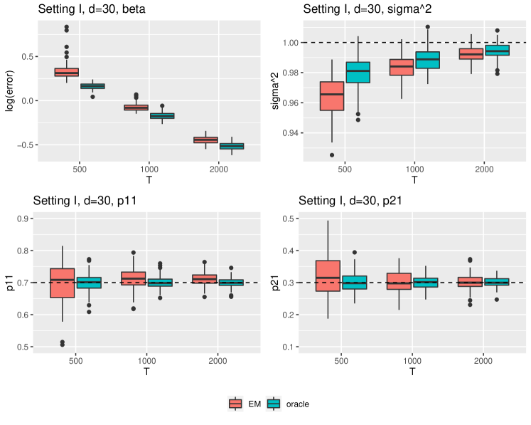
Figure 1: Estimation of regression coefficients $\beta$ (top left), conditional variance $\sigma^{2}$ (top right), transition probabilities $p_{11}$ (bottom left) and $p_{21}$ (bottom right) in Setting I with $d=30$. In the top left panel, log error is defined as $\log(\|\hat{\beta}-\beta^{*}\|_{2})$; and in the other panels, black dashed line marks the true parameter value. Results are based on 100 simulation replications.

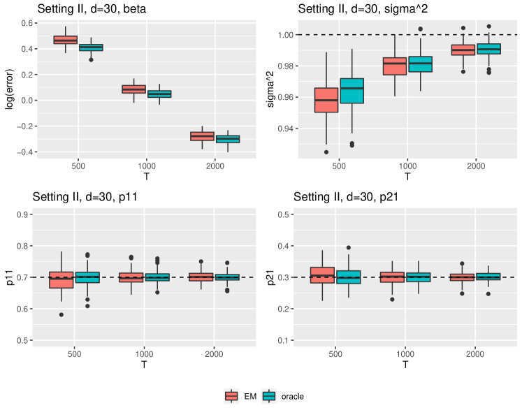
Figure 2: Estimation of regression coefficients $\beta$ (top left), conditional variance $\sigma^{2}$ (top right), transition probabilities $p_{11}$ (bottom left) and $p_{21}$ (bottom right) in Setting II with $d=30$. In the top left panel, log error is defined as $\log(\|\hat{\beta}-\beta^{*}\|_{2})$; and in the other panels, black dashed line marks the true parameter value. Results are based on 100 simulation replications.

5 Discussion

In this paper, we developed a regularized approximate EM algorithm for parameter estimation in high-dimensional Markov-switching VAR models. The proposed algorithm uses an approximation of the conditional expectation in the E-step, and allows the dimension of the outcome vector to diverge exponentially with the sample size. We also established statistical guarantees for the resulting estimate using probabilistic tools for ergodic time series.

In terms of computation, the proposed algorithm can be implemented efficiently. First, in each iteration of the EM algorithm, the approximate conditional expectations can be computed efficiently. Then, the update for $p$ in (2.2) has a closed-form solution; and the update for $\beta$ is a weighted lasso problem, which can be solved using software packages such as glmnet in R. In our theoretical derivation (see Theorem 3.5), the tuning parameter needs to be updated in each iteration. However, specifying $\lambda$ according to (3.5) is challenging, as it requires knowing the true magnitude of the estimation error. In the simulations, we choose $\lambda$ based on cross-validation in each iteration, and we found that it worked well in the simulation settings we have considered.

To the best of our knowledge, we are not aware of theoretical guarantees for the EM algorithm with arbitrary initialization. In our theory, we require that the initialization falls within a neighborhood of the true parameter value. When initial (perhaps less precise) estimates are available, the EM algorithm can be initialized using these initial estimates. We leave the development of such initial estimates in the Markov-switching VAR setting to future research. When initial estimates are not available, we found that using multiple random initializations provides a viable solution.

In our proposed algorithm, we approximate the conditional expectation of $I\{Z_{t}=j\}$ condition on $Y_{0}^{t}$, which is termed “filtered probability” of regime $j$ in, for example, Krolzig (2013). An alternative is to use “smoothed probability” (Krolzig, 2013) instead, that is, the conditional expectation of $I\{Z_{t}=j\}$ condition on the full observed data $Y_{0}^{T}$, as the observed outcomes after time $t$ may provide additional information about $Z_{t}$. This smoothed probability can be calculated exactly through a forward-backward recursion (Hamilton, 1989). However, for any time point $t$, this conditional expectation depend on all observations $Y_{0},Y_{1},\ldots,Y_{T}$, and thus it can be challenging to establish certain concentration results to derive the estimation error bound. Similar to our current proposal, approximation of the smoothed probabilities could be used. One can also consider conditioning on $(Y_{t-s}^{t+\tilde{s}},Z_{t-s})$ for some properly chosen $s$ and $\tilde{s}$ to capture additional information about $Z_{t}$. We expect that most information about $Z_{t}$ is encoded in the transition from $Y_{t-1}$ to $Y_{t}$, and the current proposal based on “filtered probabilities” would have reasonable performance. Indeed, in the simulations, we observe that the performance of our EM estimates is comparable to the oracle estimate that observes $Z_{t}$.

The proposed method can also be generalized to the case where the covariance matrix of $\epsilon_{t}$ takes a more flexible form and may be regime-dependent. With the assumption that the precision matrix is sparse, techniques for high-dimensional graphical models developed in, for example, Hao et al. (2017) could be incorporated into the current algorithm. Similar probabilistic tools can be applied to analyze the resulting estimate.

Appendix

Appendix A Additional simulation results

Figure 3 summarizes the simulation results for $d=90$, based on 20 simulation replications. The results show estimation error of $\beta$, as well as estimates of $\sigma^{2}$ and the transition probabilities in Setting I. The results are similar to those for $d=30$ presented in the main paper.

Figure 4 shows simulation results for $d=90$ in Setting II. In this case, the regression parameter has a large dimension, namely 16,200, and the magnitude of individual regression coefficient is smaller compared to the other settings. As a result, for smaller sample size, it can be difficult to find good initializations. But as sample size increases, the performance of the EM estimate improves greatly and becomes comparable to the oracle estimate.

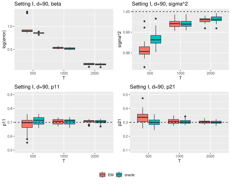
Figure 3: Estimation of regression coefficients $\beta$ (top left), conditional variance $\sigma^{2}$ (top right), transition probabilities $p_{11}$ (bottom left) and $p_{21}$ (bottom right) in Setting I with $d=90$. In the top left panel, log error is defined as $\log(\|\hat{\beta}-\beta^{*}\|_{2})$; and in the other panels, black dashed line marks the true parameter value. Results are based on 20 simulation replications.

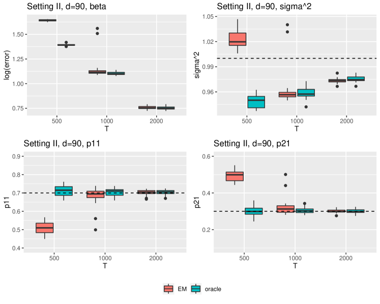
Figure 4: Estimation of regression coefficients $\beta$ (top left), conditional variance $\sigma^{2}$ (top right), transition probabilities $p_{11}$ (bottom left) and $p_{21}$ (bottom right) in Setting II with $d=90$. In the top left panel, log error is defined as $\log(\|\hat{\beta}-\beta^{*}\|_{2})$; and in the other panels, black dashed line marks the true parameter value. Results are based on 20 simulation replications.

Appendix B Signal strength in a symmetric case with i.i.d. $Z_{t}$

In this appendix, we study the (inverse) signal strength measure $\kappa$ introduced in Assumption 2 more closely in an example. Specifically, we focus on the case where the regime variables $\{Z_{t}\}$ are binary with value 1 or 2, and are independent and identically distributed over time, that is, $p_{11}=p_{21}$ in the transition matrix. Moreover, we assume that the transition probability of $Z$, $p$, is known, the variance $\sigma^{2}$ is known to be 1, and the regression coefficient matrices in the two regimes are such that $B_{1}=B$ and $B_{2}=-B$. As $B_{1}=-B_{2}$, we refer to this case as a symmetric mixture (of vector autoregression.)

Let $\beta=\textnormal{vec}(B)$, and $\beta$ is the only parameter that needs to be estimated. Hence, hereafter in Appendix B, we will write $\beta$ for the parameter vector instead of $\theta$. Let $p_{1}=P(Z_{t}=1)$ and $p_{2}=P(Z_{t}=2)$. The independence among the $Z_{t}$’s allows us to obtain a simple form for the filtered probability $w_{j,\beta}(Y_{0}^{t})$. Indeed, we have

$$w_{1,\beta}(Y_{0}^{t}) =P(Z_{t}=1|Y_{0},Y_{1},\ldots,Y_{t})=P(Z_{t}=1|Y_{t-1},Y_{t})$$

$$=\frac{P(Y_{t-1},Z_{t}=1,Y_{t})}{P(Y_{t-1},Y_{t})}=\frac{P(Z_{t}=1,Y_{t}|Y_{t-1})}{P(Y_{t}|Y_{t-1})}$$

$$=\frac{P(Y_{t}|Y_{t-1},Z_{t}=1)P(Z_{t}=1|Y_{t-1})}{\sum_{j=1}^{2}P(Y_{t}|Y_{t-1},Z_{t}=j)P(Z_{t}=j|Y_{t-1})}$$

$$=\frac{p_{1}P(Y_{t}|Y_{t-1},Z_{t}=1)}{\sum_{j=1}^{2}p_{j}P(Y_{t}|Y_{t-1},Z_{t}=j)}$$

$$=\frac{p_{1}\exp\left(-\frac{1}{2}\left\|Y_{t}-(\textnormal{Id}_{d}\otimes Y_{t-1})^{\top}\beta\right\|_{2}^{2}\right)}{p_{1}\exp\left(-\frac{1}{2}\left\|Y_{t}-(\textnormal{Id}_{d}\otimes Y_{t-1})^{\top}\beta\right\|_{2}^{2}\right)+p_{2}\exp\left(-\frac{1}{2}\left\|Y_{t}+(\textnormal{Id}_{d}\otimes Y_{t-1})^{\top}\beta\right\|_{2}^{2}\right)},$$

and $w_{2,\beta}=1-w_{1,\beta}$. As these filtered probabilities depend only on $Y_{t-1}$ and $Y_{t}$, we will write them as $w_{j,\beta}(Y_{t-1}^{t})$. By some algebra, we have the gradient of $w_{1,\beta}(Y_{t-1}^{t})$ with respect to $\beta$:

$$\frac{\partial w_{1,\beta}(Y_{t-1}^{t})}{\partial\beta} =2w_{1,\beta}(Y_{t-1}^{t})\left\{1-w_{1,\beta}(Y_{t-1}^{t})\right\}\left(\textnormal{Id}_{d}\otimes Y_{t-1}\right)Y_{t}$$

$$=2w_{1,\beta}(Y_{t-1}^{t})\left\{1-w_{1,\beta}(Y_{t-1}^{t})\right\}\left(Y_{t}\otimes Y_{t-1}\right),$$

where the second equality follows from the mixed-product property of Kronecker product.

As both $p$ and $\sigma^{2}$ are assumed to be known, we only need to optimize the following objective function in the population EM algorithm

$$Q(\tilde{\beta}|\beta) =\frac{1}{T}\sum_{t=1}^{T}E_{0}\left[-\frac{1}{2}w_{1,\beta}(Y_{0}^{t})\|Y_{t}-(\textnormal{Id}_{d}\otimes Y_{t-1})^{\top}\tilde{\beta}\|_{2}^{2}-\frac{1}{2}\left\{1-w_{1,\beta}(Y_{0}^{t})\right\}\|Y_{t}+(\textnormal{Id}_{d}\otimes Y_{t-1})^{\top}\tilde{\beta}\|_{2}^{2}\right]$$

$$=\frac{1}{T}\sum_{t=1}^{T}E_{0}\left[-\frac{1}{2}w_{1,\beta}(Y_{t-1}^{t})\|Y_{t}-(\textnormal{Id}_{d}\otimes Y_{t-1})^{\top}\tilde{\beta}\|_{2}^{2}-\frac{1}{2}\left\{1-w_{1,\beta}(Y_{t-1}^{t})\right\}\|Y_{t}+(\textnormal{Id}_{d}\otimes Y_{t-1})^{\top}\tilde{\beta}\|_{2}^{2}\right]$$

$$=E_{0}\left[-\frac{1}{2}w_{1,\beta}(Y_{t-1}^{t})\|Y_{t}-(\textnormal{Id}_{d}\otimes Y_{t-1})^{\top}\tilde{\beta}\|_{2}^{2}-\frac{1}{2}\left\{1-w_{1,\beta}(Y_{t-1}^{t})\right\}\|Y_{t}+(\textnormal{Id}_{d}\otimes Y_{t-1})^{\top}\tilde{\beta}\|_{2}^{2}\right].$$

To maximize the objective function $Q(\tilde{\beta}|\beta)$, we first take its derivative with respect to $\tilde{\beta}$,

$$\frac{\partial Q(\tilde{\beta}|\beta)}{\partial\tilde{\beta}}=-E_{0}\left[(\textnormal{Id}_{d}\otimes Y_{t-1})(\textnormal{Id}_{d}\otimes Y_{t-1})^{\top}\tilde{\beta}+\left\{1-2w_{1,\beta}(Y_{t-1}^{t})\right\}(\textnormal{Id}_{d}\otimes Y_{t-1})Y_{t}\right].$$

Setting the derivative to 0, we have that

$$M(\beta)=\left\{E_{0}\left[(\textnormal{Id}_{d}\otimes Y_{t-1})(\textnormal{Id}_{d}\otimes Y_{t-1})^{\top}\right]\right\}^{-1}E_{0}\left[\left\{2w_{1,\beta}(Y_{t-1}^{t})-1\right\}(\textnormal{Id}_{d}\otimes Y_{t-1})Y_{t}\right].$$

Consequently,

$$\frac{\partial M(\beta)}{\partial\beta} =\left\{E_{0}\left[(\textnormal{Id}_{d}\otimes Y_{t-1})(\textnormal{Id}_{d}\otimes Y_{t-1})^{\top}\right]\right\}^{-1}E_{0}\left[(\textnormal{Id}_{d}\otimes Y_{t-1})Y_{t}2\frac{\partial w_{1,\beta}(Y_{t-1}^{t})}{\partial\beta}^{\top}\right]$$

$$=\left\{E_{0}\left[(\textnormal{Id}_{d}\otimes Y_{t-1})(\textnormal{Id}_{d}\otimes Y_{t-1})^{\top}\right]\right\}^{-1}E_{0}\left[4w_{1,\beta}(Y_{t-1}^{t})\left\{1-w_{1,\beta}(Y_{t-1}^{t})\right\}(\textnormal{Id}_{d}\otimes Y_{t-1})Y_{t}\left(Y_{t}\otimes Y_{t-1}\right)^{\top}\right]$$

$$=\left\{E_{0}\left[(\textnormal{Id}_{d}\otimes Y_{t-1})(\textnormal{Id}_{d}\otimes Y_{t-1})^{\top}\right]\right\}^{-1}E_{0}\left[4w_{1,\beta}(Y_{t-1}^{t})\left\{1-w_{1,\beta}(Y_{t-1}^{t})\right\}\left(Y_{t}\otimes Y_{t-1}\right)\left(Y_{t}\otimes Y_{t-1}\right)^{\top}\right]$$

$$=\left\{E_{0}\left[\textnormal{Id}_{d}\otimes(Y_{t-1}Y_{t-1}^{\top})\right]\right\}^{-1}E_{0}\left[4w_{1,\beta}(Y_{t-1}^{t})\left\{1-w_{1,\beta}(Y_{t-1}^{t})\right\}\left(Y_{t}\otimes Y_{t-1}\right)\left(Y_{t}\otimes Y_{t-1}\right)^{\top}\right]$$

$$=\left\{\textnormal{Id}_{d}\otimes E_{0}\left[Y_{t-1}Y_{t-1}^{\top}\right]\right\}^{-1}E_{0}\left[4w_{1,\beta}(Y_{t-1}^{t})\left\{1-w_{1,\beta}(Y_{t-1}^{t})\right\}\left(Y_{t}\otimes Y_{t-1}\right)\left(Y_{t}\otimes Y_{t-1}\right)^{\top}\right]$$

where the third and fourth equality is again due to the mixed-product property of Kronecker product.

We now derive an upper bound on $\|\partial M(\beta)/\partial\beta\|_{2}$, and later we will examine this upper bound empirically. Note that the matrix $\textnormal{Id}_{d}\otimes E_{0}[Y_{t-1}Y_{t-1}^{\top}]$ is positive definite, and so is its inverse. Thus, we have that

$$\left\|\frac{\partial M(\beta)}{\partial\beta}\right\|_{2} \leq\left\|\left\{\textnormal{Id}_{d}\otimes E_{0}\left[Y_{t-1}Y_{t-1}^{\top}\right]\right\}^{-1}\right\|_{2}\left\|E_{0}\left[4w_{1,\beta}(Y_{t-1}^{t})\left\{1-w_{1,\beta}(Y_{t-1}^{t})\right\}\left(Y_{t}\otimes Y_{t-1}\right)\left(Y_{t}\otimes Y_{t-1}\right)^{\top}\right]\right\|_{2}$$

$$=\lambda_{\max}\left(\left\{\textnormal{Id}_{d}\otimes E_{0}\left[Y_{t-1}Y_{t-1}^{\top}\right]\right\}^{-1}\right)\left\|E_{0}\left[4w_{1,\beta}(Y_{t-1}^{t})\left\{1-w_{1,\beta}(Y_{t-1}^{t})\right\}\left(Y_{t}\otimes Y_{t-1}\right)\left(Y_{t}\otimes Y_{t-1}\right)^{\top}\right]\right\|_{2}$$

$$=\left\{\lambda_{\min}\left(\textnormal{Id}_{d}\otimes E_{0}\left[Y_{t-1}Y_{t-1}^{\top}\right]\right)\right\}^{-1}\left\|E_{0}\left[4w_{1,\beta}(Y_{t-1}^{t})\left\{1-w_{1,\beta}(Y_{t-1}^{t})\right\}\left(Y_{t}\otimes Y_{t-1}\right)\left(Y_{t}\otimes Y_{t-1}\right)^{\top}\right]\right\|_{2}$$

$$=\left\{\lambda_{\min}\left(E_{0}\left[Y_{t-1}Y_{t-1}^{\top}\right]\right)\right\}^{-1}\left\|E_{0}\left[4w_{1,\beta}(Y_{t-1}^{t})\left\{1-w_{1,\beta}(Y_{t-1}^{t})\right\}\left(Y_{t}\otimes Y_{t-1}\right)\left(Y_{t}\otimes Y_{t-1}\right)^{\top}\right]\right\|_{2}.$$

Define an inverse signal-to-noise ratio as

$$\textnormal{ISNR}_{\beta}=\left\{\lambda_{\min}\left(E_{0}\left[Y_{t-1}Y_{t-1}^{\top}\right]\right)\right\}^{-1}\left\|E_{0}\left[4w_{1,\beta}(Y_{t-1}^{t})\left\{1-w_{1,\beta}(Y_{t-1}^{t})\right\}\left(Y_{t}\otimes Y_{t-1}\right)\left(Y_{t}\otimes Y_{t-1}\right)^{\top}\right]\right\|_{2},$$

which is a continuous function of $\beta$.

We empirically examine the magnitude of ISNR${}_{\beta^{*}}$ in two sets of experiments as we increase the magnitude or dimension of $\beta^{*}$. In the first set of experiments, we consider a low-dimensional setting with $d=3$, and increase the magnitude of $\beta^{*}$. In particular, we define the matrix $A$ as

$$A=\begin{bmatrix}0.5&0&0\\ 0.1&0.1&0.3\\ 0&0.2&0.3\end{bmatrix},$$

and let $B^{*}=\mu A$, for a scaling factor $\mu$ that we vary from $0.3$ to $1.5$. The choice of the range of $\mu$ is such that $\|B^{*}\|_{2}$ does not exceed 1 per Assumption 1. Let $\beta^{*}=\textnormal{vec}(B^{*})$, and we examine ISNR${}_{\beta^{*}}$ as we increase $\mu$. The relevant expectations in the definition of ISNR are approximated with the corresponding sample average, using a sample of size 100,000 taken after a 50,000-step burn-in period. We set $p_{1}=p_{2}=0.5$. The results are presented in Figure 5. We observe that as the magnitude of the regression coefficients increases, the inverse signal-to-noise ratio decreases. Therefore, the ISNR is indeed a reasonable measure of signal strength, and the signal becomes strong as the magnitude of the regression coefficients becomes larger.

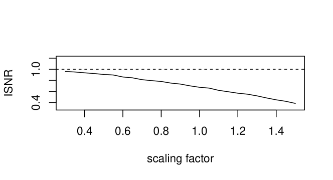
Figure 5: Inverse signal-to-noise ratio (ISNR) in a low-dimensional setting ($d=3$), when the scaling factor increases from 0.3 to 1.5. The magnitude of the regression coefficients is proportional to the scaling factor. Dashed line corresponds to ISNR being 1.

In the second set of experiments, we fix the scaling factor $\mu$ at 1, but increase the dimension $d$ from 3 to 30. We take $B^{*}=\textnormal{Id}_{d/3}\otimes A$ and $\beta^{*}=\textnormal{vec}(B^{*})$. Figure 6 plots the ISNR against the dimension. We observe that when individual diagonal block in $B^{*}$ remains the same as the dimension $d$ increases, the signal becomes stronger and the ISNR becomes smaller. Moreover, this suggests that as dimension increases, we can allow the magnitude of the difference of a individual regression coefficient between regimes to shrink and still get a non-decreasing signal-to-noise ratio.

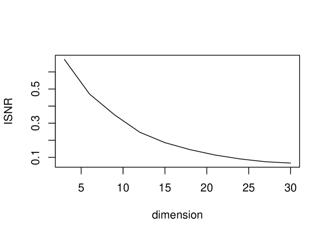
Figure 6: Inverse signal-to-noise ratio (ISNR) as dimension increases from 3 to 30, with the scaling factor fixed at 1.

We also study the expectation of $\|\frac{\partial w_{1,\beta}}{\partial\beta}\frac{\partial w_{1,\beta}}{\partial\beta}^{\top}\|_{2}^{2}$. Recall that $\frac{\partial w_{1,\beta}(Y_{t-1}^{t})}{\partial\beta}=2w_{1,\beta}(Y_{t-1}^{t})\{1-w_{1,\beta}(Y_{t-1}^{t})\}(Y_{t}\otimes Y_{t-1})$, and therfore

$$\frac{\partial w_{1,\beta}(Y_{t-1}^{t})}{\partial\beta}\frac{\partial w_{1,\beta}(Y_{t-1}^{t})}{\partial\beta}^{\top}=\left[2w_{1,\beta}(Y_{t-1}^{t})\left\{1-w_{1,\beta}(Y_{t-1}^{t})\right\}\right]^{2}\left(Y_{t}\otimes Y_{t-1}\right)\left(Y_{t}\otimes Y_{t-1}\right)^{\top}.$$

Hence,

$$\left\|\frac{\partial w_{1,\beta}(Y_{t-1}^{t})}{\partial\beta}\frac{\partial w_{1,\beta}(Y_{t-1}^{t})}{\partial\beta}^{\top}\right\|_{2}^{2} =\left[2w_{1,\beta}(Y_{t-1}^{t})\left\{1-w_{1,\beta}(Y_{t-1}^{t})\right\}\right]^{4}\left\|\left(Y_{t}\otimes Y_{t-1}\right)\left(Y_{t}\otimes Y_{t-1}\right)^{\top}\right\|_{2}^{2}$$

$$=\left[2w_{1,\beta}(Y_{t-1}^{t})\left\{1-w_{1,\beta}(Y_{t-1}^{t})\right\}\right]^{4}\left\|\left(Y_{t}\otimes Y_{t-1}\right)\right\|_{2}^{4}$$

$$=\left[2w_{1,\beta}(Y_{t-1}^{t})\left\{1-w_{1,\beta}(Y_{t-1}^{t})\right\}\right]^{4}\left\|Y_{t}\right\|_{2}^{4}\left\|Y_{t-1}\right\|_{2}^{4}.$$

We study the expectation of the quantity above when $\beta=\beta^{*}$ as we increase the magnitude of the regression coefficients or the dimension. The expectation is approximated using a sample average in the same way as described earlier. Figure 7 plots the expected squared norm as we increase the scaling factor from 0.3 to 1.5 while keeping the dimension fixed at $d=3$. Figure 8 plots the expected squared norm as we increase the dimension $d$ from 3 to 90 while keeping the scaling factor at 1. The observed trends suggest that Assumption 9 is plausible using arguments based on Markov inequality with the expectation being bounded.

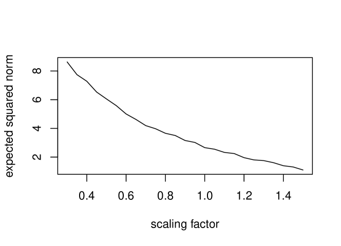
Figure 7: Expected squared norm of $(\partial w_{1,\beta}/\partial\beta)(\partial w_{1,\beta}/\partial\beta)^{\top}$ in a low-dimensional setting ($d=3$), when the scaling factor increases from 0.3 to 1.5. The magnitude of the regression coefficients is proportional to the scaling factor.

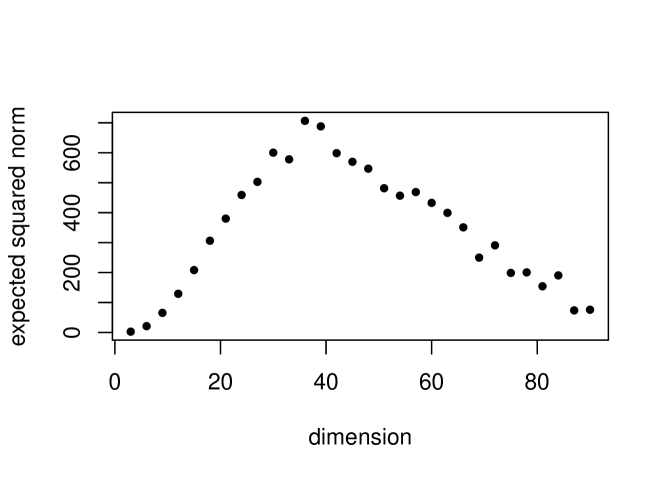
Figure 8: Expected squared norm of $(\partial w_{1,\beta}/\partial\beta)(\partial w_{1,\beta}/\partial\beta)^{\top}$ as dimension increases from 3 to 90, with the scaling factor fixed at 1.

Appendix C An expectation-maximization-truncation algorithm

To control the number of false positives in the estimate of the regression coefficients $\hat{\beta}$, we introduce an additional thresholding step. Specifically, for a given function $\xi$ of sample size $T$ and dimension $d$, we let $\xi(T,d)$ be the threshold level. Define the thresholded estimate $\hat{\beta}_{thres}$ such that $\hat{\beta}_{thres}^{k}=\hat{\beta}^{k}I\{|\hat{\beta}^{k}|\geq\xi(T,d)\}$, where $\hat{\beta}_{thres}^{k}$ and $\hat{\beta}^{k}$ denote the $k$-th element of the vector $\hat{\beta}_{thres}$ and $\hat{\beta}$, respectively, for $k\in\{1,\ldots,Kd^{2}\}$. This thresholding step allows us to control the (non-)sparsity level of the regression coefficient estimates uniformly throughout the EM iterations, and can potentially facilitate the theoretical analysis of the algorithm as discussed in Section 3.

We outline such an expectation-maximization-truncation (EMT) algorithm in Algorithm 2. The penalty parameter $\lambda$ and the threshold level $\xi$ will change over iterations, and we use $\lambda^{(q)}$ and $\xi^{(q)}$ to denote their values in the $q$-th iteration.

Algorithm 2 An EMT algorithm for high-dimensional Markov-switching VAR model

Input: Observations $\{Y_{0},Y_{1},\ldots,Y_{T}\}$, number of regimes $K$;
      Output: Parameter estimate $\hat{\theta}$

Initialize the parameter $\theta^{(0)}=(\beta^{(0)},p^{(0)},(\sigma^{(0)})^{2})$

$q\leftarrow 1$

while Convergence condition not met do

     (a) choose tuning parameter $\lambda^{(q)}$ and threshold level $\xi^{(q)}$

     (b) optimize the objective (8): $\hat{\theta}=(\hat{\beta}^{\top},\hat{p}^{\top},\hat{\sigma}^{2})^{\top}=\arg\max_{\tilde{\theta}}Q_{n,\lambda^{(q)}}(\tilde{\theta}|\theta^{(q-1)})$

     (c) update $p$ and $\sigma$: $p^{(q)}\leftarrow\hat{p}$, $\sigma^{(q)}\leftarrow\hat{\sigma}$

     (d) update $\beta$: $\beta^{(q)}\leftarrow\hat{\beta}_{thres}$ with $\hat{\beta}_{thres}^{k}=\hat{\beta}^{k}I\{|\hat{\beta}^{k}|\geq\xi^{(q)}\}$

     (e) update $\theta$: $\theta^{(q)}\leftarrow(\beta^{(q)},p^{(q)},(\sigma^{(q)})^{2})$

     $q\leftarrow q+1$

end while

$\hat{\theta}\leftarrow\theta^{(q)}$

Appendix D Useful lemmas

First we introduce an auxiliary lemma that will be useful to establish the approximation error bound in Lemma 3.3. First, consider a generic (row) stochastic matrix $M\in\mathbb{R}^{a\times b}$, that is, a matrix whose entries are all non-negative and where entries in each row sum up to 1. Following Hajnal and Bartlett [1958], we define the following quantities to measure the extent to which the rows of $M$ differ from each other. Define $\zeta(M):=\max_{1\leq i,k\leq a}\{1-\sum_{1\leq j\leq b}\min(M_{ij},M_{kj})\}$. We note that $\zeta(M)$ can be written as

$$\zeta(M) =\max_{1\leq i,k\leq a}\{1-\sum_{1\leq j\leq b}\min(M_{ij},M_{kj})\}$$

$$=\max_{1\leq i,k\leq a}\{\sum_{1\leq j\leq b}M_{ij}-\sum_{1\leq j\leq b}\min(M_{ij},M_{kj})\}$$

$$=\max_{1\leq i,k\leq a}\sum_{j:M_{ij}>M_{kj}}(M_{ij}-M_{kj}),$$

and therefore $\zeta(M)$ is zero if and only if the rows of $M$ are all the same. Define $\psi(M):=\max_{1\leq i,k\leq a}\max_{1\leq j\leq b}|M_{ij}-M_{kj}|$. Again, $\psi(M)=0$ if and only if the rows of $M$ are all the same. The following lemma establishes an important property of these measures.

Lemma D.1 (Lemma 3 in Hajnal and Bartlett [1958]).

If $M=M_{1}M_{2}$ where $M_{1}$ and $M_{2}$ are both stochastic matrices, then $\psi(M)\leq\zeta(M_{1})\psi(M_{2})$.

Next, we state a key concentration result for $\beta$-mixing processes that we will apply when proving the restricted eigenvalue condition.

Lemma D.2 (Adapted from Lemma 13 of Wong et al. [2020]; see also Merlevède et al. [2011]).

Let $\{X_{t}\}_{t=1}^{T}$ be a strictly stationary sequence of mean zero random variables that are subweibull$(\gamma_{2})$ with subweibull constant $K_{X}$. Denote their sum by $S_{T}$. Suppose their $\beta$-mixing coefficients satisfy $b_{\textnormal{mix}}(l)\leq 2\exp(-c(l-s)^{\gamma_{1}})$ for $l\geq s$ and $s\leq C\log(T)$ for some constant $C$. Let $\gamma$ be a parameter given by $\gamma=(1/\gamma_{1}+1/\gamma_{2})^{-1}$, and further assume $\gamma<1$. Then for $T>4$ and any $t>T^{-1/2}$,

$$P\left(\left|S_{T}/T\right|>t\right)\leq T\exp\left\{-\frac{(tT)^{\gamma}}{K_{X}^{\gamma}C_{1}}\right\}+\exp\left\{-\frac{t^{2}T}{K_{X}^{2}C_{2}}\right\},$$ (18)

where the constants $C_{1}$ and $C_{2}$ depend only on $\gamma_{1}$, $\gamma_{2}$ and $c$.

Appendix E Proof of lemmas in Section 3

In this section, we prove lemmas in Section 3 of the main paper.

Proof of Lemma 3.1.

Under Assumption 1, stationarity follows by directly applying Theorem 3.1 and Corollary 3.1 in Stelzer [2009], and geometric ergodicity follows by applying Theorem 5.1 and Proposition 5.3 in Stelzer [2009].

It remains to show that $Y_{t}$ is a sub-Gaussian random vector. We start by noting that Theorem 4.2 in Stelzer [2009] implies that all moments of $Y_{t}$ exist. Iteratively applying (1), we have that

$$Y_{t} =\left(\sum_{i=1}^{K}I\{Z_{t}=i\}B_{i}^{\top}\right)Y_{t-1}+\epsilon_{t}$$

$$=\left(\sum_{i=1}^{K}I\{Z_{t}=i\}B_{i}^{\top}\right)\left(\sum_{i=1}^{K}I\{Z_{t-1}=i\}B_{i}^{\top}\right)Y_{t-2}+\left(\sum_{i=1}^{K}I\{Z_{t}=i\}B_{i}^{\top}\right)\epsilon_{t-1}+\epsilon_{t}$$

$$=\left(\sum_{i=1}^{K}I\{Z_{t}=i\}B_{i}^{\top}\right)\left(\sum_{i=1}^{K}I\{Z_{t-1}=i\}B_{i}^{\top}\right)\left(\sum_{i=1}^{K}I\{Z_{t-2}=i\}B_{i}^{\top}\right)Y_{t-3}$$

$$\quad\left(\sum_{i=1}^{K}I\{Z_{t}=i\}B_{i}^{\top}\right)\left(\sum_{i=1}^{K}I\{Z_{t-1}=i\}B_{i}^{\top}\right)\epsilon_{t-2}+\left(\sum_{i=1}^{K}I\{Z_{t}=i\}B_{i}^{\top}\right)\epsilon_{t-1}+\epsilon_{t}$$

$$=\cdots$$

$$=\left[\prod_{k=0}^{J}\left(\sum_{i=1}^{K}I\{Z_{t-k}=i\}B_{i}^{\top}\right)\right]Y_{t-J-1}+\sum_{l=1}^{J}\left[\prod_{k=0}^{l-1}\left(\sum_{i=1}^{K}I\{Z_{t-k}=i\}B_{i}^{\top}\right)\epsilon_{t-l}\right]+\epsilon_{t},$$

for any positive integer $J$. For a generic time point $t$, we define the matrix $A_{t}=\sum_{i=1}^{K}I\{Z_{t}=i\}B_{i}^{\top}$. Although the matrix $A_{t}$ is random due to the randomness in $Z_{t}$, Assumption 1 implies that $\|A_{t}\|_{2}\leq\tilde{c}$ with probability 1. With the definition of $A_{t}$, the above display can be written equivalently as

$$Y_{t}=\left(\prod_{k=0}^{J}A_{t-k}\right)Y_{t-J-1}+\sum_{l=1}^{J}\left\{\left(\prod_{k=0}^{l-1}A_{t-k}\right)\epsilon_{t-l}\right\}+\epsilon_{t}.$$

In fact, we can continue expanding $Y_{t}$, and Theorem 4.2 in Stelzer [2009] implies that the stationary distribution of $Y_{t}$ admits the following representation

$$Y_{t}=\sum_{l=1}^{\infty}\left\{\left(\prod_{k=0}^{l-1}A_{t-k}\right)\epsilon_{t-l}\right\}+\epsilon_{t},$$

where the series on the right-hand side in the above display converges in the norm $\|\cdot\|_{L^{r}}$ for any $r\geq 1$, with the norm defined as $(E\|X\|_{2}^{r})^{1/r}$ for a random vector $X$.

Since $\epsilon_{t}$ follows a Gaussian distribution, there exists a constant $K_{1}>0$ such that for all $v\in\mathbb{R}^{d}$ with $\|v\|_{2}=1$,

$$\left(E\left|v^{\top}\epsilon_{t}\right|^{p}\right)^{1/p}\leq K_{1}p^{1/2}.$$ (19)

Now fix an arbitrary unit-vector $v\in\mathbb{R}^{d}$. For the ease of notation, we introduce a truncated version of the series representation of $Y_{t}$ defined as $Y_{t}^{J}=\sum_{l=1}^{J}\{(\prod_{k=0}^{l-1}A_{t-k})\epsilon_{t-l}\}+\epsilon_{t}$, for a positive integer $J$. By Minkowski inequality,

$$\left(E\left|v^{\top}Y_{t}\right|^{p}\right)^{1/p} \leq\underbrace{\left(E\left|v^{\top}\left(Y_{t}-Y_{t}^{J}\right)\right|^{p}\right)^{1/p}}_{\textnormal{term a}}+\underbrace{\sum_{l=1}^{J}\left(E\left|v^{\top}\left(\prod_{k=0}^{l-1}A_{t-k}\right)\epsilon_{t-l}\right|^{p}\right)^{1/p}}_{\textnormal{term b}}+\underbrace{\left(E\left|v^{\top}\epsilon_{t}\right|^{p}\right)^{1/p}}_{\textnormal{term c}}.$$

We study each term in the above display separately. First, term c is upper bounded by $K_{1}p^{1/2}$ as $\epsilon_{t}$ is a Gaussian random vector. For term a, we note that

$$\textnormal{term a}\leq\left(E\left[\|v\|_{2}^{p}\left\|Y_{t}-Y_{t}^{J}\right\|_{2}^{p}\right]\right)^{1/p}=\left(E\left\|Y_{t}-Y_{t}^{J}\right\|_{2}^{p}\right)^{1/p}=\|Y_{t}-Y_{t}^{J}\|_{L^{p}}.$$

We now study term b. To start, we note that $\epsilon_{t-l}$ is independent of $\{Z_{t-l+1},\ldots,Z_{t}\}$, and hence independent of the random matrices $A_{t-l+1},\ldots,A_{t}$. Now define a random vector $U_{t,l}=(\prod_{k=0}^{l-1}A_{t-k})^{\top}v$. Then, each term in the sum in term b is equivalent to $(E|U_{t,l}^{\top}\epsilon_{t-l}|^{p})^{1/p}$. Note that

$$E\left|U_{t,l}^{\top}\epsilon_{t-l}\right|^{p} =E\left[\left|\epsilon_{t-l}^{\top}\frac{U_{t,l}}{\|U_{t,l}\|_{2}}\right|^{p}\|U_{t,l}\|_{2}^{p}\right]$$

$$=E\left[E\left[\left|\epsilon_{t-l}^{\top}\frac{U_{t,l}}{\|U_{t,l}\|_{2}}\right|^{p}\mid Z_{t-l+1},\ldots,Z_{t}\right]\|U_{t,l}\|_{2}^{p}\right].$$

Here, condition on $\{Z_{t-l+1},\ldots,Z_{t}\}$, the vector $U_{t,l}$ becomes deterministic, but the distribution of $\epsilon_{t-l}$ is unchanged due to the independence. Thus,

$$E\left[\left|\epsilon_{t-l}^{\top}\frac{U_{t,l}}{\|U_{t,l}\|_{2}}\right|^{p}\mid Z_{t-l+1},\ldots,Z_{t}\right]\leq\left(K_{1}p^{1/2}\right)^{p},$$

and consequently

$$E\left|U_{t,l}^{\top}\epsilon_{t-l}\right|^{p}\leq\left(K_{1}p^{1/2}\right)^{p}E\left[\|U_{t,l}\|_{2}^{p}\right].$$

The norm $\|U_{t,l}\|_{2}$ is upper bounded by $\prod_{k=0}^{l-1}\|A_{t-k}\|_{2}$, which is upper bounded by $\tilde{c}^{l}$ with probability 1. Thus, $E\left[\|U_{t,l}\|_{2}^{p}\right]\leq\tilde{c}^{lp}$. Combining these results, we get that

$$\left(E\left|v^{\top}\left(\prod_{k=0}^{l-1}A_{t-k}\right)\epsilon_{t-l}\right|^{p}\right)^{1/p}\leq\tilde{c}^{l}K_{1}p^{1/2}.$$

Putting the upper bounds for terms a, b and c together, we have

$$\left(E\left|v^{\top}Y_{t}\right|^{p}\right)^{1/p} \leq\|Y_{t}-Y_{t}^{J}\|_{L^{p}}+\sum_{l=1}^{J}\tilde{c}^{l}K_{1}p^{1/2}+K_{1}p^{1/2}$$

$$=\|Y_{t}-Y_{t}^{J}\|_{L^{p}}+\frac{1-\tilde{c}^{J+1}}{1-\tilde{c}}K_{1}p^{1/2}.$$

The above display holds for any positive integer $J$, and hence we can take the limit as $J$ approaches infinity. By Theorem 4.2 in Stelzer [2009], $\|Y_{t}-Y_{t}^{J}\|_{L^{p}}$ converges to 0 and thus,

$$\left(E\left|v^{\top}Y_{t}\right|^{p}\right)^{1/p}\leq\frac{1}{1-\tilde{c}}K_{1}p^{1/2},$$

which implies that $Y_{t}$ is a sub-Gaussian random vector.

∎

Proof of Lemma 3.2.

This lemma follows directly from the mean-value inequality and the fact that $M(\theta^{*})=\theta^{*}$. ∎

Proof of Lemma 3.3.

For generic $t_{1}<t_{2}\leq t$, define matrix $P^{t_{1},t_{2}}\in\mathbb{R}^{K\times K}$ with the $(i,j)$-th entry

$$(P^{t_{1},t_{2}})_{ij}=P_{\theta}(Z_{t_{2}}=j|Y_{t_{1}},\ldots,Y_{t},Z_{t_{1}}=i).$$

Note that regardless of the values of $t_{1},t_{2}$, we always condition on the outcome vectors $Y$ until time $t$. Recall that

$$m_{j,\theta}(Y_{t-s},\ldots,Y_{t})=P_{\theta}(Z_{t}=j|Y_{t-s},\ldots,Y_{t},Z_{t-s}=1),$$

which, with our new definition, can be equivalently written as $(P^{t-s,t})_{1j}$. Meanwhile, we can write $w_{j,\theta}$ as follows.

$$\quad w_{j,\theta}(Y_{0},\ldots,Y_{t})$$

$$=P(Z_{t}=j|Y_{0},\ldots,Y_{t})$$

$$=\sum_{i}P(Z_{t}=j|Y_{0},\ldots,Y_{t},Z_{t-s}=i)P(Z_{t-s}=i|Y_{0},\ldots,Y_{t})$$

$$=\sum_{i}P(Z_{t}=j|Y_{t-s},\ldots,Y_{t},Z_{t-s}=i)P(Z_{t-s}=i|Y_{0},\ldots,Y_{t})$$

$$=\sum_{i}P(Z_{t}=j|Y_{t-s},\ldots,Y_{t},Z_{t-s}=1)P(Z_{t-s}=i|Y_{0},\ldots,Y_{t})$$

$$\quad+\sum_{i}\{P(Z_{t}=j|Y_{t-s},\ldots,Y_{t},Z_{t-s}=i)-P(Z_{t}=j|Y_{t-s},\ldots,Y_{t},Z_{t-s}=1)\}P(Z_{t-s}=i|Y_{0},\ldots,Y_{t})$$

$$=(P^{t-s,t})_{1j}+\sum_{i}\{(P^{t-s,t})_{ij}-(P^{t-s,t})_{1j}\}P(Z_{t-s}=i|Y_{0},\ldots,Y_{t}).$$

Hence,

$$|w_{j,\theta}(Y_{0},\ldots,Y_{t})-m_{j,\theta}(Y_{t-s},\ldots,Y_{t})| =\left|\sum_{i}\{(P^{t-s,t})_{ij}-(P^{t-s,t})_{1j}\}P(Z_{t-s}=i|Y_{0},\ldots,Y_{t})\right|$$

$$\leq\sum_{i}\left|(P^{t-s,t})_{ij}-(P^{t-s,t})_{1j}\right|P(Z_{t-s}=i|Y_{0},\ldots,Y_{t})$$

$$\leq\max_{i,k}\max_{j}|(P^{t-s,t})_{ij}-(P^{t-s,t})_{kj}|\sum_{i}P(Z_{t-s}=i|Y_{0},\ldots,Y_{t})$$

$$=\psi(P^{t-s,t}),$$

where $\psi(\cdot)$ is defined in Appendix D. Thus, if we can show that $\psi(P^{t-s,t})\leq\phi^{s}$, we can get the desired result that $|w_{j,\theta}(Y_{0},\ldots,Y_{t})-m_{j,\theta}(Y_{t-s},\ldots,Y_{t})|\leq\phi^{s}$.

Next, we show that under the assumptions of Lemma 3.3, we indeed have $\psi(P^{t-s,t})\leq\phi^{s}$. To this end, we first note that condition on $Y$’s, $\{Z_{t}\}$ form a time-inhomogeneous Markov chain, and thus

$$P^{t-s,t}=P^{t-s,t-s+1}P^{t-s+1,t-s+2}\cdots P^{t-2,t-1}P^{t-1,t}.$$

By Lemma D.1, it suffices to show that $\zeta(P^{t_{1},t_{1}+1})\leq\phi$ for generic $t_{1}<t$, where $\zeta(\cdot)$ is defined in Appendix D. Note that we can take the stochastic matrix on the very right in Lemma D.1 to be the identity matrix, and $\psi(\textnormal{Id}_{K})=1$. By Bayes rule,

$$(P^{t_{1},t_{1}+1})_{ij} =P(Z_{t_{1}+1}=j|Y_{t_{1}},\ldots,Y_{t},Z_{t_{1}}=i)$$

$$=\frac{P(Z_{t_{1}}=i,Y_{t_{1}},Z_{t_{1}+1}=j,Y_{t_{1}+1},Y_{t_{1}+2}\ldots,Y_{t})}{P(Z_{t_{1}}=i,Y_{t_{1}},Y_{t_{1}+1},\ldots,Y_{t})}$$

$$=\frac{P(Z_{t_{1}}=i,Y_{t_{1}},Z_{t_{1}+1}=j,Y_{t_{1}+1},\ldots,Y_{t})}{\sum_{l}P(Z_{t_{1}}=i,Y_{t_{1}},Z_{t_{1}+1}=l,Y_{t_{1}+1},\ldots,Y_{t},)}$$

$$=\frac{\sum_{z_{t_{1}+2},\ldots,z_{t}}P_{ij}p_{j}(Y_{t_{1}+1}|Y_{t_{1}})P_{jz_{t_{1}+2}}p_{z_{t_{1}+2}}(Y_{t_{1}+2}|Y_{t_{1}+1})\ldots P_{z_{t-1}z_{t}}p_{z_{t}}(Y_{t}|Y_{t-1})}{\sum_{l}\sum_{z_{t_{1}+2},\ldots,z_{t}}P_{il}p_{l}(Y_{t_{1}+1}|Y_{t_{1}})P_{lz_{t_{1}+2}}p_{z_{t_{1}+2}}(Y_{t_{1}+2}|Y_{t_{1}+1})\ldots P_{z_{t-1}z_{t}}p_{z_{t}}(Y_{t}|Y_{t-1})},$$

where $p_{j}(\cdot|\cdot)$ denotes the conditional density function of $Y_{t+1}|(Y_{t},Z_{t}=j)$, for $j\in\{1,\ldots,K\}$. Let $\Pi=\{(z_{t_{1}+2},\ldots,z_{t}):z_{t_{1}+2},\ldots,z_{t}\in\{1,\ldots,K\}\}$. Furthermore, for $l\in\{1,\ldots,K\}$ and $\pi\in\Pi$, define

$$f_{l\pi}=p_{l}(Y_{t_{1}+1}|Y_{t_{1}})P_{lz_{t_{1}+2}}p_{z_{t_{1}+2}}(Y_{t_{1}+2}|Y_{t_{1}+1})\ldots P_{z_{t-1}z_{t}}p_{z_{t}}(Y_{t}|Y_{t-1}).$$

Then,

$$(P^{t_{1},t_{1}+1})_{ij}=\frac{\sum_{\pi\in\Pi}P_{ij}f_{j\pi}}{\sum_{l}\sum_{\pi\in\Pi}P_{il}f_{l\pi}}.$$

Thus,

$$(P^{t_{1},t_{1}+1})_{ij}-(P^{t_{1},t_{1}+1})_{kj} =\frac{\sum_{\pi\in\Pi}P_{ij}f_{j\pi}}{\sum_{l}\sum_{\pi\in\Pi}P_{il}f_{l\pi}}-\frac{\sum_{\tilde{\pi}\in\Pi}P_{kj}f_{j\tilde{\pi}}}{\sum_{\tilde{l}}\sum_{\tilde{\pi}\in\Pi}P_{k\tilde{l}}f_{\tilde{l}\tilde{\pi}}}$$

$$=\frac{\sum_{\pi\in\Pi}\sum_{\tilde{\pi}\in\Pi}\left[P_{ij}f_{j\pi}\sum_{\tilde{l}}P_{k\tilde{l}}f_{\tilde{l}\tilde{\pi}}-P_{kj}f_{j\tilde{\pi}}\sum_{l}P_{il}f_{l\pi}\right]}{\sum_{\pi\in\Pi}\sum_{\tilde{\pi}\in\Pi}\left[\sum_{l}P_{il}f_{l\pi}\sum_{\tilde{l}}P_{k\tilde{l}}f_{\tilde{l}\tilde{\pi}}\right]}$$

$$\leq\frac{\sum_{\pi\in\Pi}\sum_{\tilde{\pi}\in\Pi}\sum_{l\neq j}\left(P_{ij}f_{j\pi}P_{kl}f_{l\tilde{\pi}}-P_{kj}f_{j\tilde{\pi}}P_{il}f_{l\pi}\right)}{\sum_{\pi\in\Pi}\sum_{\tilde{\pi}\in\Pi}\sum_{l\neq j}\left(P_{il}f_{l\pi}P_{kj}f_{j\tilde{\pi}}+P_{ij}f_{j\pi}P_{kl}f_{l\tilde{\pi}}\right)}$$

$$=\frac{\sum_{\pi\in\Pi}\sum_{\tilde{\pi}\in\Pi}\sum_{l\neq j}\left(P_{ij}f_{j\tilde{\pi}}P_{kl}f_{l\pi}-P_{kj}f_{j\tilde{\pi}}P_{il}f_{l\pi}\right)}{\sum_{\pi\in\Pi}\sum_{\tilde{\pi}\in\Pi}\sum_{l\neq j}\left(P_{il}f_{l\pi}P_{kj}f_{j\tilde{\pi}}+P_{ij}f_{j\tilde{\pi}}P_{kl}f_{l\pi}\right)}.$$

Thus,

$$|(P^{t_{1},t_{1}+1})_{ij}-(P^{t_{1},t_{1}+1})_{kj}| \leq\frac{\sum_{\pi\in\Pi}\sum_{\tilde{\pi}\in\Pi}\sum_{l\neq j}\left|P_{ij}f_{j\tilde{\pi}}P_{kl}f_{l\pi}-P_{kj}f_{j\tilde{\pi}}P_{il}f_{l\pi}\right|}{\sum_{\pi\in\Pi}\sum_{\tilde{\pi}\in\Pi}\sum_{l\neq j}\left(P_{il}f_{l\pi}P_{kj}f_{j\tilde{\pi}}+P_{ij}f_{j\tilde{\pi}}P_{kl}f_{l\pi}\right)}$$

$$\leq\frac{\sum_{\pi\in\Pi}\sum_{\tilde{\pi}\in\Pi}\sum_{l\neq j}\left\{\left(P_{il}f_{l\pi}P_{kj}f_{j\tilde{\pi}}+P_{ij}f_{j\tilde{\pi}}P_{kl}f_{l\pi}\right)\max_{l\neq j}\frac{\left|P_{ij}P_{kl}-P_{il}P_{kj}\right|}{\left(P_{ij}P_{kl}+P_{il}P_{kj}\right)}\right\}}{\sum_{\pi\in\Pi}\sum_{\tilde{\pi}\in\Pi}\sum_{l\neq j}\left(P_{il}f_{l\pi}P_{kj}f_{j\tilde{\pi}}+P_{ij}f_{j\tilde{\pi}}P_{kl}f_{l\pi}\right)}$$

$$=\max_{l\neq j}\frac{\left|P_{ij}P_{kl}-P_{il}P_{kj}\right|}{\left(P_{ij}P_{kl}+P_{il}P_{kj}\right)}.$$

Recall that

$$\zeta(P^{t_{1},t_{1}+1})=\max_{1\leq i,k\leq K}\sum_{j:(P^{t_{1},t_{1}+1})_{ij}>(P^{t_{1},t_{1}+1})_{kj}}((P^{t_{1},t_{1}+1})_{ij}-(P^{t_{1},t_{1}+1})_{kj}),$$

which implies that

$$\zeta(P^{t_{1},t_{1}+1}) \leq\max_{1\leq i,k\leq K}\sum_{j}|(P^{t_{1},t_{1}+1})_{ij}-(P^{t_{1},t_{1}+1})_{kj}|$$

$$\leq\max_{1\leq i,k\leq K}\sum_{j=1}^{K}\max_{l\neq j}\frac{\left|P_{ij}P_{kl}-P_{il}P_{kj}\right|}{\left(P_{ij}P_{kl}+P_{il}P_{kj}\right)}$$

$$\leq\phi,$$

where the last line follows from Assumption 4.

The approximation error of $m_{ij,\theta}$ can be upper bounded in a similar fashion. Specifically, recall that

$$m_{ij,\theta}(Y_{t-s}^{t})=P_{\theta}(Z_{t-1}=i,Z_{t}=j|Z_{t-s}=1,Y_{t-s},\ldots,Y_{t}),$$

and

$$w_{ij,\theta}(Y_{0}^{t})=P_{\theta}(Z_{t-1}=i,Z_{t}=j|Y_{0},Y_{1},\ldots,Y_{t}).$$

Then, the approximation error can be written as

$$\quad w_{ij,\theta}(Y_{0}^{t})-m_{ij,\theta}(Y_{t-s}^{t})$$

$$=P_{\theta}(Z_{t-1}=i,Z_{t}=j|Y_{0},Y_{1},\ldots,Y_{t})-P_{\theta}(Z_{t-1}=i,Z_{t}=j|Z_{t-s}=1,Y_{t-s},\ldots,Y_{t})$$

$$=\sum_{k=1}^{K}P_{\theta}(Z_{t-1}=i,Z_{t}=j|Z_{t-s}=k,Y_{0},Y_{1},\ldots,Y_{t})P_{\theta}(Z_{t-s}=k|Y_{0},Y_{1},\ldots,Y_{t})$$

$$\quad-P_{\theta}(Z_{t-1}=i,Z_{t}=j|Z_{t-s}=1,Y_{t-s},\ldots,Y_{t})$$

$$=\sum_{k=1}^{K}P_{\theta}(Z_{t-1}=i,Z_{t}=j|Z_{t-s}=k,Y_{t-s},\ldots,Y_{t})P_{\theta}(Z_{t-s}=k|Y_{0},Y_{1},\ldots,Y_{t})$$

$$\quad-P_{\theta}(Z_{t-1}=i,Z_{t}=j|Z_{t-s}=1,Y_{t-s},\ldots,Y_{t})$$

$$=\sum_{k=1}^{K}P_{\theta}(Z_{t}=j|Z_{t-1}=i,Y_{t-1},Y_{t})P_{\theta}(Z_{t-1}=i|Z_{t-s}=k,Y_{t-s},\ldots,Y_{t})P_{\theta}(Z_{t-s}=k|Y_{0},Y_{1},\ldots,Y_{t})$$

$$\quad-P_{\theta}(Z_{t}=j|Z_{t-1}=i,Y_{t-1},Y_{t})P_{\theta}(Z_{t-1}=i|Z_{t-s}=1,Y_{t-s},\ldots,Y_{t})$$

$$=P_{\theta}(Z_{t}=j|Z_{t-1}=i,Y_{t-1},Y_{t})$$

$$\quad\left[\sum_{k=1}^{K}\left\{P_{\theta}(Z_{t-1}=i|Z_{t-s}=k,Y_{t-s},\ldots,Y_{t})-P_{\theta}(Z_{t-1}=i|Z_{t-s}=1,Y_{t-s},\ldots,Y_{t})\right\}P_{\theta}(Z_{t-s}=k|Y_{0},Y_{1},\ldots,Y_{t})\right].$$

Hence,

$$\left|w_{ij,\theta}(Y_{0}^{t})-m_{ij,\theta}(Y_{t-s}^{t})\right| \leq\max_{k}\left|P_{\theta}(Z_{t-1}=i|Z_{t-s}=k,Y_{t-s},\ldots,Y_{t})-P_{\theta}(Z_{t-1}=i|Z_{t-s}=1,Y_{t-s},\ldots,Y_{t})\right|$$

$$=(P^{t-s,t-1})_{ki}-(P^{t-s,t-1})_{1i}\leq\psi(P^{t-s,t-1}).$$

Again, we have

$$P^{t-s,t-1}=P^{t-s,t-s+1}P^{t-s+1,t-s+2}\cdots P^{t-2,t-1},$$

and $\psi(P^{t-s,t-1})\leq\phi^{s-1}$ if $\zeta(P^{t_{1},t_{1}+1})\leq\phi$ for generic $t_{1}$. ∎

Appendix F Proof of Lemma 3.4

Proof of Lemma 3.4.

Recall that in this lemma, we aim to show that for all $j\in\{1,\ldots,K\}$ and all $v\in\mathbb{R}^{d^{2}}$,

$$v^{\top}\left[\frac{1}{T}\sum_{t=1}^{T}\textnormal{Id}_{d}\otimes\left\{m_{j,\theta}(Y_{t-s}^{t})Y_{t-1}Y_{t-1}^{\top}\right\}\right]v\geq\alpha\|v\|_{2}^{2}-\tau_{RE}\|v\|_{1}^{2},$$

uniformly over $\theta\in\Theta$, with high probability. We first give an outline of the proof. We start by controlling the tail behavior of $v^{\top}\{m_{j,\theta}(Y_{t-s}^{t})Y_{t-1}Y_{t-1}^{\top}\}v$, which will enable us to obtain a uniform concentration results over $\theta$ over a collection of sparse vectors $v$, if $\{Y_{t}\}_{t=1}^{T}$ were independent and identically distributed. Under $\beta$-mixing, this translates to a uniform concentration result for our original time series data, which leads to a lower bound on $v^{\top}\left[\frac{1}{T}\sum_{t=1}^{T}\textnormal{Id}_{d}\otimes\left\{m_{j,\theta}(Y_{t-s}^{t})Y_{t-1}Y_{t-1}^{\top}\right\}\right]v$ for sparse $v$. We will then show that this lower bound for sparse vectors implies a lower bound for all vectors $v$. In the following, we present the complete proof.

First, Lemma B.1 in Basu and Michailidis [2015] implies that it suffices to show that

$$v^{\top}\left[\frac{1}{T}\sum_{t=1}^{T}m_{j,\theta}(Y_{t-s}^{t})Y_{t-1}Y_{t-1}^{\top}\right]v\geq\alpha\|v\|_{2}^{2}-\tau_{RE}\|v\|_{1}^{2},$$

for all $v\in\mathbb{R}^{d}$ uniformly over $\theta$. We will prove the above statement under the assumptions of Lemma 3.4 in the following steps.

Step I: control the tail behavior of $v^{\top}\{m_{j,\theta}(Y_{t-s}^{t})Y_{t-1}Y_{t-1}^{\top}\}v$. To start, we recall that under the stationary distribution, $Y_{t}$ is a sub-Gaussian random vector and we define

$$K_{Y}=\sup_{v\in\mathbb{R}^{d},\|v\|_{2}=1}\sup_{q\geq 1}(E|v^{\top}Y_{t}|^{q})^{1/q}q^{-1/2}.$$

Therefore,

$$E|v^{\top}Y_{t}|^{q}\leq K_{Y}^{q}q^{q/2},\quad\forall q\geq 1,\ \forall v\in\mathbb{R}^{d},\ \|v\|_{2}=1.$$ (20)

This implies that

$$E\left[\left\{m_{j,\theta}(Y_{t-s}^{t})v^{\top}Y_{t-1}Y_{t-1}^{\top}v\right\}^{q}\right] =E\left[\left\{m_{j,\theta}(Y_{t-s}^{t})\right\}^{q}\left\{v^{\top}Y_{t-1}Y_{t-1}^{\top}v\right\}^{q}\right]$$

$$\leq E\left[\left\{v^{\top}Y_{t-1}Y_{t-1}^{\top}v\right\}^{q}\right]$$

$$=E\left[\left|v^{\top}Y_{t-1}\right|^{2q}\right]$$

$$\leq K_{Y}^{2q}(2q)^{q},$$

and therefore

$$\left(E\left[\left\{m_{j,\theta}(Y_{t-s}^{t})v^{\top}Y_{t-1}Y_{t-1}^{\top}v\right\}^{q}\right]\right)^{1/q}\leq 2K_{Y}^{2}q.$$

Step II: uniform concentration for i.i.d data with sparse $v$. For a vector $v\in\mathbb{R}^{d}$, let $\textnormal{supp}(v)\subseteq\{1,\ldots,d\}$ denote the support of $v$, that is, $\textnormal{supp}(v)=\{i:v_{i}\neq 0\}$. Let $\mathbb{S}(2b)=\{v\in\mathbb{R}^{d}:|\textnormal{supp}(v)|\leq 2b,\|v\|_{2}\leq 1\}$ denote the set of $2b$-sparse vectors in the $d$-dimensional unit ball. We will specify the exact value of $b$ in a later step. For any subset $\tilde{S}$ of $\{1,\ldots,d\}$ with cardinality $2b$, let $\mathbb{S}_{\tilde{S}}$ denote the subset of $\mathbb{S}(2b)$ supported on $\tilde{S}$. Let $\mathbb{K}_{\tilde{S}}$ be a $1/10$-cover of $\mathbb{S}_{\tilde{S}}$, and define $\mathbb{K}=\cup_{\tilde{S}}\mathbb{K}_{\tilde{S}}$. Then, $\mathbb{K}$ is a $1/10$-cover of $\mathbb{S}(2b)$. Since the $\epsilon$ covering number of a $2b$-dimensional unit ball is upper bounded by $(3/\epsilon)^{2b}$, we have $|\mathbb{K}|\leq\binom{d}{2b}30^{2b}$. Here, the binomial coefficient $\binom{d}{2b}$ arises from the fact that $v\in\mathbb{S}(2b)$ is supported on one of the $\binom{d}{2b}$ subsets of cardinality $2b$ of $\{1,\ldots,d\}$.

Define a function $f_{v,\theta}^{j}$ as

$$f_{v,\theta}^{j}(Y_{t-s}^{t})=m_{j,\theta}(Y_{t-s}^{t})v^{\top}Y_{t-1}Y_{t-1}^{\top}v,$$

and define a function class

$$\mathcal{F}=\left\{f_{v,\theta}^{j}:j\in\{1,\ldots,K\},v\in\mathbb{K},\theta\in\Theta\right\}.$$

We now establish a uniform concentration result over the function class $\mathcal{F}$ for i.i.d. data. To this end, for a fixed constant $\tilde{c}$, let $N=T/\{\tilde{c}\log T\}$. Let $\{\tilde{Y}_{n-s}^{n}\}_{n=1}^{N}$ be an i.i.d. sample where the marginal distribution of $\tilde{Y}_{n-s}^{n}$ is the same as the marginal distribution of $Y_{t-s}^{t}$. For the ease of notation, let $X_{n}=\tilde{Y}_{n-s}^{n}$. Note that the sample size of this i.i.d. sample is smaller than the sample size of the original time series by a log factor, and the reason for this shall become clear in later steps of the proof. We study the following tail probability

$$P\left(\sup_{f\in\mathcal{F}}\left|\frac{1}{N}\sum_{n=1}^{N}f(X_{n})-E[f(X_{n})]\right|>\frac{\rho_{\min}}{243}\right),$$

where $\rho_{\min}$ is defined in Assumption 5.

Step II-I: symmetrization. We start with a symmetrization argument using Theorem G.1. To apply this theorem, we first need to find an upper bound for the $L_{2}$ norm of functions in $\mathcal{F}$. For any fixed function $f\in\mathcal{F}$, there exist $j\in\{1,\ldots,K\}$, $v\in\mathbb{K}$ and $\theta\in\Theta$ such that

$$\|f\|_{2}^{2} =E\left[f(X_{n})^{2}\right]=E\left[m_{j,\theta}(Y_{t-s}^{t})^{2}\left\{v^{\top}Y_{t-1}Y_{t-1}^{\top}v\right\}^{2}\right]$$

$$\leq E\left[\left\{v^{\top}Y_{t-1}Y_{t-1}^{\top}v\right\}^{2}\right]$$

$$\leq 16K_{Y}^{4},$$

where the second line follows from the fact that $m_{j,\theta}$ is uniformly upper bounded by 1, and the third line follows from our result from Step I. The upper bound above holds for any $v$, $j$ and $\theta$. Thus, we can take $R=4K_{Y}^{2}$ in Theorem G.1. Now to apply this theorem, we only need that $T\geq 72\tilde{c}(\log T)(972K_{Y}^{2}/\rho_{\min})^{2}$. Note that this holds for sufficiently large $T$. Under this condition, Theorem G.1 implies that

$$P\left(\sup_{f\in\mathcal{F}}\left|\frac{1}{N}\sum_{n=1}^{N}f(X_{n})-E[f(X_{n})]\right|>\frac{\rho_{\min}}{243}\right)\leq 4P\left(\sup_{f\in\mathcal{F}}\left|\frac{1}{N}\sum_{n=1}^{N}W_{n}f(X_{n})\right|\geq\frac{\rho_{\min}}{972}\right).$$

Step II-II: Control the empirical norm of functions in $\mathcal{F}$. To control the probability on the right-hand side of the above display, we first condition on $X_{1},\ldots,X_{N}$. Define the event $\mathcal{A}$ such that $I_{\mathcal{A}}\{X_{1},\ldots,X_{N}\}=1$ if and only if

$$\sup_{f\in\mathcal{F}}\frac{1}{N}\sum_{n=1}^{N}f(X_{n})^{2}\leq 16K_{Y}^{4}+1.$$

We now study the probability of the event $\mathcal{A}$. For a fixed vector $v\in\mathbb{K}$, define a function class

$$\mathcal{F}_{v}=\left\{f_{v,\theta}^{j}:j\in\{1,\ldots,K\},\theta\in\Theta\right\}.$$

With this definition, the function class $\mathcal{F}$ can be written as $\mathcal{F}=\cup_{v\in\mathbb{K}}\mathcal{F}_{v}$.

$$\sup_{f\in\mathcal{F}_{v}}\frac{1}{N}\sum_{n=1}^{N}f(X_{n})^{2} =\max_{j}\sup_{\theta\in\Theta}\frac{1}{N}\sum_{n=1}^{N}m_{j,\theta}(\tilde{Y}_{t-s}^{t})^{2}\left\{v^{\top}\tilde{Y}_{t-1}\tilde{Y}_{t-1}^{\top}v\right\}^{2}$$

$$\leq\max_{j}\sup_{\theta\in\Theta}\frac{1}{N}\sum_{n=1}^{N}\left\{v^{\top}\tilde{Y}_{t-1}\tilde{Y}_{t-1}^{\top}v\right\}^{2}$$

$$=\frac{1}{N}\sum_{n=1}^{N}\left\{v^{\top}\tilde{Y}_{t-1}\tilde{Y}_{t-1}^{\top}v\right\}^{2}.$$

As shown in Step I, for any fixed vector $v$, the random variable $v^{\top}\tilde{Y}_{t-1}\tilde{Y}_{t-1}^{\top}v$ is sub-weibull$(1)$ with sub-weibull norm $2K_{Y}^{2}$. By Lemma 6 in Wong et al. [2020], $\{v^{\top}\tilde{Y}_{t-1}\tilde{Y}_{t-1}^{\top}v\}^{2}$ is sub-weibull$(1/2)$ with sub-weibull norm $16K_{Y}^{4}$. Now by Lemma D.2,

$$P\left(\left|\frac{1}{N}\sum_{n=1}^{N}\left\{v^{\top}\tilde{Y}_{t-1}\tilde{Y}_{t-1}^{\top}v\right\}^{2}-E\left[\left\{v^{\top}\tilde{Y}_{t-1}\tilde{Y}_{t-1}^{\top}v\right\}^{2}\right]\right|>1\right)\leq N\exp\left\{-\frac{N^{1/2}}{4K_{Y}^{2}\tilde{C}_{1}}\right\}+\exp\left\{-\frac{N}{256K_{Y}^{8}\tilde{C}_{2}}\right\},$$

for some constants $\tilde{C}_{1}$ and $\tilde{C}_{2}$. As we have shown, $E[\{v^{\top}\tilde{Y}_{t-1}\tilde{Y}_{t-1}^{\top}v\}^{2}]\leq 16K_{Y}^{4}$. Together with the above display, this implies that

$$P\left(\frac{1}{N}\sum_{n=1}^{N}\left\{v^{\top}\tilde{Y}_{t-1}\tilde{Y}_{t-1}^{\top}v\right\}^{2}>16K_{Y}^{4}+1\right)\leq N\exp\left\{-\frac{N^{1/2}}{4K_{Y}^{2}\tilde{C}_{1}}\right\}+\exp\left\{-\frac{N}{256K_{Y}^{8}\tilde{C}_{2}}\right\},$$

and therefore

$$P\left(\sup_{f\in\mathcal{F}_{v}}\frac{1}{N}\sum_{n=1}^{N}f(X_{n})^{2}>16K_{Y}^{4}+1\right)\leq N\exp\left\{-\frac{N^{1/2}}{4K_{Y}^{2}\tilde{C}_{1}}\right\}+\exp\left\{-\frac{N}{256K_{Y}^{8}\tilde{C}_{2}}\right\},$$

for a fixed $v\in\mathbb{K}$. Applying a union bound over $\mathbb{K}$, we have that

$$P\left(\sup_{f\in\mathcal{F}}\frac{1}{N}\sum_{n=1}^{N}f(X_{n})^{2}>16K_{Y}^{4}+1\right)\leq\binom{d}{2b}30^{2b}N\exp\left\{-\frac{N^{1/2}}{4K_{Y}^{2}\tilde{C}_{1}}\right\}+\binom{d}{2b}30^{2b}\exp\left\{-\frac{N}{256K_{Y}^{8}\tilde{C}_{2}}\right\}.$$

This provides a way to control the empirical norm of functions in the class $\mathcal{F}$ uniformly with high probability.

Step II-III: condition on $X_{1},\ldots,X_{N}$. We now condition on $X_{1},\ldots,X_{N}$ and study the probability

$$P\left(\sup_{f\in\mathcal{F}}\left|\frac{1}{N}\sum_{n=1}^{N}W_{n}f(X_{n})\right|\geq\frac{\rho_{\min}}{972}\mid X_{1}=x_{1},\ldots,X_{N}=x_{N},I_{\mathcal{A}}\left\{X_{1},\ldots,X_{N}\right\}=1\right).$$

for a set of values $x_{1},\ldots,x_{N}$ such that $I_{\mathcal{A}}\{x_{1},\ldots,x_{N}\}=1$. Our main tool to control the probability above is Corollary 8.3 in van de Geer [2000], which requires controlling the entropy of the function class $\mathcal{F}$.

By a Sudakov minoration argument similar to the proof of Proposition 3.6, we have

$$\sqrt{\log N_{c}(\epsilon,\Theta,\|\cdot\|_{2})}\leq C_{1}r\sqrt{|S|(\log K+\log d)}/\epsilon,$$

for some constant $C_{1}$. Now consider the function class $\mathcal{F}_{v}^{j}=\{f_{v,\theta}^{j}:\theta\in\Theta\}$. We aim to relate the entropy of $\mathcal{F}_{v}^{j}$ to that of $\Theta$, by showing that functions in $\mathcal{F}_{v}^{j}$ are Lipschitz with respect to $\theta$. Let $Q_{n}(x_{1},\ldots,x_{N})$ denote the empirical distribution that puts mass $1/N$ at each value $x_{n}$. We will often omit in the notation its dependence on $(x_{1},\ldots,x_{N})$ and write $Q_{n}$ for simplicity. For a function $f$, define its norm under $Q_{n}$, $\|f\|_{Q_{n}}$, such that $\|f\|_{Q_{n}}^{2}=\int f^{2}dQ_{n}=\sum_{n=1}^{N}f^{2}(x_{n})/N$.

$$\left\|f_{v,\theta_{1}}^{j}-f_{v,\theta_{1}}^{j}\right\|_{Q_{n}}^{2} =\frac{1}{N}\sum_{n=1}^{N}\left\{f_{v,\theta_{1}}^{j}(\tilde{Y}_{n-s}^{n})-f_{v,\theta_{2}}^{j}(\tilde{Y}_{n-s}^{n})\right\}^{2}$$

$$=\frac{1}{N}\sum_{n=1}^{N}\left\{m_{j,\theta_{1}}(\tilde{Y}_{n-s}^{n})v^{\top}\tilde{Y}_{n-1}\tilde{Y}_{n-1}^{\top}v-m_{j,\theta_{2}}(\tilde{Y}_{n-s}^{n})v^{\top}\tilde{Y}_{n-1}\tilde{Y}_{n-1}^{\top}v\right\}^{2}$$

$$=\frac{1}{N}\sum_{n=1}^{N}\left\{v^{\top}\tilde{Y}_{n-1}\tilde{Y}_{n-1}^{\top}v\right\}^{2}\left\{\int_{0}^{1}\frac{\partial m_{j,\theta}(\tilde{Y}_{n-s}^{n})}{\partial\theta}\rvert_{\theta=u\theta_{1}+(1-u)\theta_{2}}^{\top}(\theta_{2}-\theta_{1})du\right\}^{2}$$

$$\leq\left[\frac{1}{N}\sum_{n=1}^{N}\left\{v^{\top}\tilde{Y}_{n-1}\tilde{Y}_{n-1}^{\top}v\right\}^{4}\right]^{1/2}\left[\frac{1}{N}\sum_{n=1}^{N}\left\{\int_{0}^{1}\frac{\partial m_{j,\theta}(\tilde{Y}_{n-s}^{n})}{\partial\theta}\rvert_{\theta=u\theta_{1}+(1-u)\theta_{2}}^{\top}(\theta_{2}-\theta_{1})du\right\}^{4}\right]^{1/2},$$

where the last line follows from Cauchy-Schwarz inequality. The first term in the last line is upper bounded by some constant uniformly in $v$ with high probability. To see this, we apply Lemma 6 in Wong et al. [2020] again and get that $\{v^{\top}\tilde{Y}_{n-1}\tilde{Y}_{n-1}^{\top}v\}^{4}$ is sub-weibull$(1/4)$ with sub-weibull norm $K_{4,Y}=2^{4}(16K_{Y}^{4})^{2}$. Applying Lemma D.2, we get the following concentration result:

$$P\left(\left|\frac{1}{N}\sum_{n=1}^{N}\left\{v^{\top}\tilde{Y}_{n-1}\tilde{Y}_{n-1}^{\top}v\right\}^{4}-E\left[\left\{v^{\top}\tilde{Y}_{n-1}\tilde{Y}_{n-1}^{\top}v\right\}^{4}\right]\right|>1\right)\leq N\exp\left(-\frac{N^{1/4}}{K_{4,Y}^{1/4}\tilde{C}_{1}}\right)+\exp\left(-\frac{N}{K_{4,Y}^{2}\tilde{C}_{2}}\right),$$

for $N\geq 4$. Recall that we have shown in step I that $E[\{v^{\top}\tilde{Y}_{n-1}\tilde{Y}_{n-1}^{\top}v\}^{4}]\leq 8^{4}K_{Y}^{8}$ for all $v\in\mathbb{K}$. Combined with the above concentration result, we have that

$$P\left(\frac{1}{N}\sum_{n=1}^{N}\left\{v^{\top}\tilde{Y}_{n-1}\tilde{Y}_{n-1}^{\top}v\right\}^{4}>1+8^{4}K_{Y}^{8}\right)\leq N\exp\left(-\frac{N^{1/4}}{K_{4,Y}^{1/4}\tilde{C}_{1}}\right)+\exp\left(-\frac{N}{K_{4,Y}^{2}\tilde{C}_{2}}\right),$$

for any fixed $v\in\mathbb{K}$. Applying a union bound over $\mathbb{K}$, we have that

$$P\left(\sup_{v\in\mathbb{K}}\frac{1}{N}\sum_{n=1}^{N}\left\{v^{\top}\tilde{Y}_{n-1}\tilde{Y}_{n-1}^{\top}v\right\}^{4}>1+8^{4}K_{Y}^{8}\right)\leq\binom{d}{2b}30^{2b}N\exp\left(-\frac{N^{1/4}}{K_{4,Y}^{1/4}\tilde{C}_{1}}\right)+\binom{d}{2b}30^{2b}\exp\left(-\frac{N}{K_{4,Y}^{2}\tilde{C}_{2}}\right).$$

We now turn to the second term,

$$\quad\left[\frac{1}{N}\sum_{n=1}^{N}\left\{\int_{0}^{1}\frac{\partial m_{j,\theta}(\tilde{Y}_{n-s}^{n})}{\partial\theta}\rvert_{\theta=u\theta_{1}+(1-u)\theta_{2}}^{\top}(\theta_{2}-\theta_{1})du\right\}^{4}\right]^{1/2}$$

$$\leq\left[\frac{1}{N}\sum_{n=1}^{N}\int_{0}^{1}\left\{\frac{\partial m_{j,\theta}(\tilde{Y}_{n-s}^{n})}{\partial\theta}\rvert_{\theta=u\theta_{1}+(1-u)\theta_{2}}^{\top}(\theta_{2}-\theta_{1})\right\}^{4}du\right]^{1/2}$$

$$=\left[\frac{1}{N}\sum_{n=1}^{N}\int_{0}^{1}\left\{(\theta_{2}-\theta_{1})^{\top}\frac{\partial m_{j,\theta}(\tilde{Y}_{n-s}^{n})}{\partial\theta}\rvert_{\theta=u\theta_{1}+(1-u)\theta_{2}}\frac{\partial m_{j,\theta}(\tilde{Y}_{n-s}^{n})}{\partial\theta}\rvert_{\theta=u\theta_{1}+(1-u)\theta_{2}}^{\top}(\theta_{2}-\theta_{1})\right\}^{2}du\right]^{1/2}$$

$$=\left[\int_{0}^{1}\frac{1}{N}\sum_{n=1}^{N}\left\{(\theta_{2}-\theta_{1})^{\top}\frac{\partial m_{j,\theta}(\tilde{Y}_{n-s}^{n})}{\partial\theta}\rvert_{\theta=u\theta_{1}+(1-u)\theta_{2}}\frac{\partial m_{j,\theta}(\tilde{Y}_{n-s}^{n})}{\partial\theta}\rvert_{\theta=u\theta_{1}+(1-u)\theta_{2}}^{\top}(\theta_{2}-\theta_{1})\right\}^{2}du\right]^{1/2}$$

$$\leq\left[\int_{0}^{1}\frac{1}{N}\sum_{n=1}^{N}\left\|\frac{\partial m_{j,\theta}(\tilde{Y}_{n-s}^{n})}{\partial\theta}\rvert_{\theta=u\theta_{1}+(1-u)\theta_{2}}\frac{\partial m_{j,\theta}(\tilde{Y}_{n-s}^{n})}{\partial\theta}\rvert_{\theta=u\theta_{1}+(1-u)\theta_{2}}^{\top}\right\|_{2}^{2}\|\theta_{2}-\theta_{1}\|_{2}^{4}du\right]^{1/2}$$

$$=\left[\int_{0}^{1}\frac{1}{N}\sum_{n=1}^{N}\left\|\frac{\partial m_{j,\theta}(\tilde{Y}_{n-s}^{n})}{\partial\theta}\rvert_{\theta=u\theta_{1}+(1-u)\theta_{2}}\frac{\partial m_{j,\theta}(\tilde{Y}_{n-s}^{n})}{\partial\theta}\rvert_{\theta=u\theta_{1}+(1-u)\theta_{2}}^{\top}\right\|_{2}^{2}du\right]^{1/2}\|\theta_{2}-\theta_{1}\|_{2}^{2}$$

$$\leq\sup_{\tilde{\theta}\in\mathcal{B}(r,\theta^{*})}\left[\frac{1}{N}\sum_{n=1}^{N}\left\|\frac{\partial m_{j,\theta}(\tilde{Y}_{n-s}^{n})}{\partial\theta}\rvert_{\theta=\tilde{\theta}}\frac{\partial m_{j,\theta}(\tilde{Y}_{n-s}^{n})}{\partial\theta}\rvert_{\theta=\tilde{\theta}}^{\top}\right\|_{2}^{2}\right]^{1/2}\|\theta_{2}-\theta_{1}\|_{2}^{2}.$$

Define a Lipschitz constant $L(x_{1}^{N})$ such that

$$L^{2}(x_{1}^{N})=\left(1+64K_{Y}^{4}\right)\max_{j}\sup_{\tilde{\theta}\in\mathcal{B}(r,\theta^{*})}\left[\frac{1}{N}\sum_{n=1}^{N}\left\|\frac{\partial m_{j,\theta}(\tilde{Y}_{n-s}^{n})}{\partial\theta}\rvert_{\theta=\tilde{\theta}}\frac{\partial m_{j,\theta}(\tilde{Y}_{n-s}^{n})}{\partial\theta}\rvert_{\theta=\tilde{\theta}}^{\top}\right\|_{2}^{2}\right]^{1/2},$$

and then we have

$$\left\|f_{v,\theta_{1}}^{j}-f_{v,\theta_{1}}^{j}\right\|_{Q_{n}}^{2}\leq L^{2}(x_{1}^{N})\|\theta_{2}-\theta_{1}\|_{2}^{2}.$$

Therefore, we can construct an $\epsilon L(x_{1}^{N})$-cover of the function class $\mathcal{F}_{v}^{j}$ from an $\epsilon$-cover of $\Theta$. As a result,

$$\sqrt{\log N_{c}(\epsilon L(x_{1}^{N}),\mathcal{F}_{v}^{j},\|\cdot\|_{Q_{n}})}\leq\sqrt{\log N_{c}(\epsilon,\Theta,\|\cdot\|_{2})}\leq\frac{C_{1}r\sqrt{|S|(\log K+\log d)}}{\epsilon},$$

and

$$\sqrt{\log N_{c}(\epsilon,\mathcal{F}_{v}^{j},\|\cdot\|_{Q_{n}})}\leq\frac{C_{1}rL(x_{1}^{N})\sqrt{|S|(\log K+\log d)}}{\epsilon}.$$

As $\mathcal{F}=\cup_{j,v}\mathcal{F}_{v}^{j}$, we have that

$$\sqrt{\log N_{c}(\epsilon,\mathcal{F},\|\cdot\|_{Q_{n}})}\leq\sqrt{\log K+\log\binom{d}{2b}+2b\log 30}+\sqrt{\log N_{c}(\epsilon,\mathcal{F}_{v}^{j},\|\cdot\|_{Q_{n}})}.$$

We are now ready to apply Theorem G.3. If $I_{A}\{x_{1},\ldots,x_{N}\}=1$, we can take $R^{2}=\max\{16K_{Y}^{4}+1,(\rho_{\min}/972)^{2}\}$ which guarantees that $R\geq\rho_{\min}/972$. We now compute the entropy integral,

$$\int_{(\rho_{\min}/972)/8}^{R}\sqrt{\log N_{c}(\epsilon,\mathcal{F},\|\cdot\|_{Q_{n}})}d\epsilon \leq C_{2}\sqrt{\log K+\log\binom{d}{2b}+2b\log 30}$$

$$\quad+C_{1}rL(x_{1}^{N})\sqrt{|S|(\log K+\log d)}\int_{(\rho_{\min}/972)/8}^{R}\frac{1}{\epsilon}d\epsilon$$

$$\leq C_{2}\sqrt{\log K+\log\binom{d}{2b}+2b\log 30}$$

$$\quad+C_{3}rL(x_{1}^{N})\sqrt{|S|(\log K+\log d)}.$$

When the following holds,

$$\sqrt{N}\geq 1944C\rho_{\min}^{-1}\max\left\{\rho_{\min}/972,4K_{Y}^{2}+1,C_{2}\sqrt{\log K+\log\binom{d}{2b}+2b\log 30}+C_{3}rL(x_{1}^{N})\sqrt{|S|(\log K+\log d)}\right\},$$ (21)

Theorem G.3 implies that

$$P\left(\sup_{f\in\mathcal{F}}\left|\frac{1}{N}\sum_{n=1}^{N}W_{n}f(x_{n})\right|\geq\frac{\rho_{\min}}{972}\right)\leq C\exp\left\{-\left(\frac{\rho_{\min}}{972}\right)^{2}\frac{N}{4C^{2}\max\{16K_{Y}^{4}+1,(\rho_{\min}/972)^{2}\}}\right\}.$$

Step II-IV: marginalize over $X_{1},\ldots,X_{N}$. Let $\mathcal{A}_{1}$ denote the event that

$$\sqrt{N}\geq 3888C\rho_{\min}^{-1}C_{3}rL(x_{1}^{N})\sqrt{|S|(\log K+\log d)}.$$

Suppose that $T$ is such that

$$\sqrt{N}\geq 1944C\rho_{\min}^{-1}\max\left\{\rho_{\min}/972,4K_{Y}^{2}+1,2C_{2}\sqrt{\log K+\log\binom{d}{2b}+2b\log 30}\right\},$$

and that $\mathcal{A}_{1}$ happens, then (21) is met. In the previous step, we derived an upper bound on the tail probability of interest, conditioned on $(x_{1},\ldots,x_{N})$ such that $I_{\mathcal{A}}=1$ and $I_{\mathcal{A}_{1}}=1$. In this step, we marginalize over $(X_{1},\ldots,X_{N})$. For two events $E_{1}$ and $E_{2}$, let $E_{1}\wedge E_{2}$ denote the event that $E_{1}$ and $E_{2}$ both happen, and $E_{1}\vee E_{2}$ denote the event that at least one of $E_{1}$ and $E_{2}$ happens. Then, we have

$$\quad P\left(\sup_{f\in\mathcal{F}}\left|\frac{1}{N}\sum_{n=1}^{N}W_{n}f(X_{n})\right|\geq\frac{\rho_{\min}}{972}\right)$$

$$\leq P\left(\sup_{f\in\mathcal{F}}\left|\frac{1}{N}\sum_{n=1}^{N}W_{n}f(X_{n})\right|\geq\frac{\rho_{\min}}{972}\wedge\mathcal{A}\wedge\mathcal{A}_{1}\right)+P(\mathcal{A}^{C})+P(\mathcal{A}_{1}^{C})$$

$$\leq C\exp\left\{-\left(\frac{\rho_{\min}}{972}\right)^{2}\frac{N}{4C^{2}\max\{16K_{Y}^{4}+1,(\rho_{\min}/972)^{2}\}}\right\}$$

$$\quad+\binom{d}{2b}30^{2b}N\exp\left\{-\frac{N^{1/2}}{4K_{Y}^{2}\tilde{C}_{1}}\right\}+\binom{d}{2b}30^{2b}\exp\left\{-\frac{N}{256K_{Y}^{8}\tilde{C}_{2}}\right\}$$

$$\quad+\binom{d}{2b}30^{2b}N\exp\left(-\frac{N^{1/4}}{K_{4,Y}^{1/4}\tilde{C}_{1}}\right)+\binom{d}{2b}30^{2b}\exp\left(-\frac{N}{K_{4,Y}^{2}\tilde{C}_{2}}\right)$$

$$\quad+\tilde{u}(N,d)$$

$$:=\tilde{u}_{RE}(N,d).$$

Combined with the symmetrization result we obtained from step II-I, we have that

$$P\left(\sup_{f\in\mathcal{F}}\left|\frac{1}{N}\sum_{n=1}^{N}f(X_{n})-E[f(X_{n})]\right|>\frac{\rho_{\min}}{243}\right)\leq 4\tilde{u}_{RE}(N,d).$$

Step III: uniform concentration for $\beta$-mixing process with sparse $v$. Now we extend the above uniform concentration results to the process $\{Y_{t-s}^{t}\}$ by applying Theorem G.4. The detailed argument is the same as in the proof of Proposition 3.6.

$$P\left(\sup_{f\in\mathcal{F}}\left|\frac{1}{T}\sum_{t=1}^{T}f(Y_{t-s}^{t})-E[f(Y_{t-s}^{t})]\right|>\frac{\rho_{\min}}{243}\right)\leq C_{3}(\log T)\tilde{u}_{RE}(N,d)+\frac{2}{T^{1/2}},$$

for some constant $C_{3}$.

Step IV: extension to all vectors $v$. For every $v\in\mathbb{S}(2b)$, there exists some $\tilde{v}(v)\in\mathbb{K}$ such that $\|v-\tilde{v}(v)\|\leq 1/10$ and that $v$ and $\tilde{v}(v)$ have the same support. For ease of notation, define

$$\Delta_{\Sigma,\theta}^{j}:=\frac{1}{T}\sum_{i=1}^{T}m_{j,\theta}(Y_{t-s}^{t})Y_{t-1}Y_{t-1}^{\top}-E\left[\frac{1}{T}\sum_{i=1}^{T}m_{j,\theta}(Y_{t-s}^{t})Y_{t-1}Y_{t-1}^{\top}\right].$$

Then, for a fixed $\theta$,

$$V:=\sup_{v\in\mathbb{S}(2b)}|v^{\top}\Delta_{\Sigma,\theta}^{j}v| =\sup_{v\in\mathbb{S}(2b)}|(v-\tilde{v}(v))^{\top}\Delta_{\Sigma,\theta}^{j}(v-\tilde{v}(v))+\tilde{v}(v)^{\top}\Delta_{\Sigma,\theta}^{j}\tilde{v}(v)+2(v-\tilde{v}(v))^{\top}\Delta_{\Sigma,\theta}^{j}\tilde{v}(v)|$$

$$\leq\sup_{v\in\mathbb{S}(2b)}|(v-\tilde{v}(v))^{\top}\Delta_{\Sigma,\theta}^{j}(v-\tilde{v}(v))|+\max_{\tilde{v}\in\mathbb{K}}|\tilde{v}^{\top}\Delta_{\Sigma,\theta}^{j}\tilde{v}|+2\sup_{v\in\mathbb{S}(2b)}|(v-\tilde{v}(v))^{\top}\Delta_{\Sigma,\theta}^{j}\tilde{v}(v)|.$$

The first term in the last line is upper bounded by $V/100$ as $10(v-\tilde{v}(v))\in\mathbb{S}(2b)$ for all $v\in\mathbb{S}(2b)$. Now consider the third term. First we note that

$$2(v-\tilde{v}(v))^{\top}\Delta_{\Sigma,\theta}^{j}(v-\tilde{v}(v))=\frac{1}{10}[\{\tilde{v}(v)+10(v-\tilde{v}(v))\}^{\top}\Delta_{\Sigma,\theta}^{j}\{\tilde{v}(v)+10(v-\tilde{v}(v))\}\\ -\tilde{v}(v)^{\top}\Delta_{\Sigma,\theta}^{j}\tilde{v}(v)-10(v-\tilde{v}(v))^{\top}\Delta_{\Sigma,\theta}^{j}\{10(v-\tilde{v}(v))\}].$$

And so,

$$2\sup_{v\in\mathbb{S}(2b)}|(v-\tilde{v}(v))^{\top}\Delta_{\Sigma,\theta}^{j}\tilde{v}(v)| \leq\frac{1}{10}\sup|\{\tilde{v}(v)+10(v-\tilde{v}(v))\}^{\top}\Delta_{\Sigma,\theta}^{j}\{\tilde{v}(v)+10(v-\tilde{v}(v))\}|$$

$$\ \ +\frac{1}{10}\sup|\tilde{v}(v)^{\top}\Delta_{\Sigma,\theta}^{j}\tilde{v}(v)|+\frac{1}{10}\sup|10(v-\tilde{v}(v))^{\top}\Delta_{\Sigma,\theta}^{j}\{10(v-\tilde{v}(v))\}|$$

$$\leq\frac{4}{10}\sup\left|\left\{\frac{\tilde{v}(v)+10(v-\tilde{v}(v))}{2}\right\}^{\top}\Delta_{\Sigma,\theta}^{j}\left\{\frac{\tilde{v}(v)+10(v-\tilde{v}(v))}{2}\right\}\right|$$

$$\ \ +\frac{1}{10}\sup|\tilde{v}(v)^{\top}\Delta_{\Sigma,\theta}^{j}\tilde{v}(v)|+\frac{1}{10}\sup|10(v-\tilde{v}(v))^{\top}\Delta_{\Sigma,\theta}^{j}\{10(v-\tilde{v}(v))\}|$$

$$\leq\frac{4}{10}V+\frac{1}{10}V+\frac{1}{10}V,$$

where the last inequality above follows from the fact that $\{\tilde{v}(v)+10(v-\tilde{v}(v))\}/2$, $\tilde{v}(v)$ and $10(v-\tilde{v}(v))$ all have norm at most 1 and hence lie in $\mathbb{S}(2b)$. Re-arranging terms, we have that

$$V\leq\frac{100}{39}\max_{\tilde{v}\in\mathbb{K}}|\tilde{v}^{\top}\Delta_{\Sigma,\theta}^{j}\tilde{v}|\leq 3\max_{\tilde{v}\in\mathbb{K}}|\tilde{v}^{\top}\Delta_{\Sigma,\theta}^{j}\tilde{v}|.$$

The above argument holds for any $\theta\in\Theta$ and $j$, and thus

$$\max_{j}\sup_{\theta\in\Theta}\sup_{v\in\mathbb{S}(2b)}|v^{\top}\Delta_{\Sigma,\theta}^{j}v|\leq 3\max_{j}\sup_{\theta\in\Theta}\max_{\tilde{v}\in\mathbb{K}}|\tilde{v}^{\top}\Delta_{\Sigma,\theta}^{j}\tilde{v}|=3\sup_{f\in\mathcal{F}}\left|\frac{1}{T}\sum_{t=1}^{T}f(Y_{t-s}^{t})-E[f(Y_{t-s}^{t})]\right|.$$

Therefore, with probability at least

$$1-C_{3}(\log T)\tilde{u}_{RE}(N,d)-\frac{2}{T^{1/2}},$$

we have that

$$\left|\frac{1}{T}\sum_{i=1}^{T}m_{j,\theta}(Y_{t-s}^{t})v^{\top}Y_{t-1}Y_{t-1}^{\top}v-E\left[m_{j,\theta}(Y_{t-s}^{t})v^{\top}Y_{t-1}Y_{t-1}^{\top}v\right]\right|\leq\frac{\rho_{\min}}{81},$$

for all $j\in\{1,\ldots,K\}$, $\theta\in\Theta$ and $v\in\mathbb{S}^{2b}$.

Next, Lemma 12 in Loh and Wainwright [2012] implies that, with probability at least

$$1-C_{3}(\log T)\tilde{u}_{RE}(N,d)-\frac{2}{T^{1/2}},$$

we have that

$$\left|\frac{1}{T}\sum_{i=1}^{T}m_{j,\theta}(Y_{t-s}^{t})v^{\top}Y_{t-1}Y_{t-1}^{\top}v-E\left[m_{j,\theta}(Y_{t-s}^{t})v^{\top}Y_{t-1}Y_{t-1}^{\top}v\right]\right|\leq\frac{\rho_{\min}}{3}\left(\|v\|_{2}^{2}+\|v\|_{1}^{2}/b\right),$$

for all $v\in\mathbb{R}^{d}$, $j\in\{1,\ldots,K\}$ and $\theta\in\Theta$. The above display implies that

$$v^{\top}\left[\frac{1}{T}\sum_{i=1}^{T}m_{j,\theta}(Y_{t-s}^{t})Y_{t-1}Y_{t-1}^{\top}\right]v \geq v^{\top}E\left[\frac{1}{T}\sum_{i=1}^{T}m_{j,\theta}(Y_{t-s}^{t})Y_{t-1}Y_{t-1}^{\top}\right]v-\frac{\rho_{\min}}{3}(\|v\|_{2}^{2}+\|v\|_{1}^{2}/b)$$

Next we relate $m_{j,\theta}$ back to $w_{j,\theta}$. In particular

$$\left|v^{\top}E\left[\frac{1}{T}\sum_{i=1}^{T}m_{j,\theta}(Y_{t-s}^{t})Y_{t-1}Y_{t-1}^{\top}\right]v-v^{\top}E\left[\frac{1}{T}\sum_{i=1}^{T}w_{j,\theta}(Y_{0}^{t})Y_{t-1}Y_{t-1}^{\top}\right]v\right|$$

$$\quad=\left|v^{\top}E\left[\frac{1}{T}\sum_{i=1}^{T}\left\{m_{j,\theta}(Y_{t-s}^{t})-w_{j,\theta}(Y_{0}^{t})\right\}Y_{t-1}Y_{t-1}^{\top}\right]v\right|$$

$$\leq\|v\|_{2}^{2}\left\|E\left[\frac{1}{T}\sum_{i=1}^{T}\left\{m_{j,\theta}(Y_{t-s}^{t})-w_{j,\theta}(Y_{0}^{t})\right\}Y_{t-1}Y_{t-1}^{\top}\right]\right\|_{2}$$

$$\leq\phi^{s}\|v\|_{2}^{2}\|E[Y_{t-1}Y_{t-1}^{\top}]\|_{2}$$

$$\leq\phi^{s}\rho_{\max}\|v\|_{2}^{2}.$$

Hence,

$$v^{\top}E\left[\frac{1}{T}\sum_{i=1}^{T}m_{j,\theta}(Y_{t-s}^{t})Y_{t-1}Y_{t-1}^{\top}\right]v \geq v^{\top}E\left[\frac{1}{T}\sum_{i=1}^{T}w_{j,\theta}(Y_{0}^{t})Y_{t-1}Y_{t-1}^{\top}\right]v-\phi^{s}\rho_{\max}\|v\|_{2}^{2}$$

$$\geq\left(\rho_{\min}-\phi^{s}\rho_{\max}\right)\|v\|_{2}^{2}\geq 2\rho_{\min}\|v\|_{2}^{2}/3,$$

when $s\asymp\log T$ and $T>\exp\{\log(\rho_{\min}/(3\rho_{\max}))/\log\phi\}$. This implies that

$$v^{\top}\left[\frac{1}{T}\sum_{i=1}^{T}m_{j,\theta}(Y_{t-s}^{t})Y_{t-1}Y_{t-1}^{\top}\right]v\geq\frac{\rho_{\min}}{3}\|v\|_{2}^{2}-\frac{\rho_{\min}}{3b}\|v\|_{1}^{2},$$

for all $v$, $j$ and $\theta$.

Step V: choose $b$ and conclusion of the proof. So far, we have shown that

$$v^{\top}\left[\frac{1}{T}\sum_{i=1}^{T}m_{j,\theta}(Y_{t-s}^{t})Y_{t-1}Y_{t-1}^{\top}\right]v\geq\frac{\rho_{\min}}{3}\|v\|_{2}^{2}-\frac{\rho_{\min}}{3b}\|v\|_{1}^{2},$$

for all $v\in\mathbb{R}^{d}$, $j\in\{1,\ldots,K\}$ and $\theta\in\Theta$, with probability at least

$$1-\frac{2}{T^{1/2}}-C_{3}(\log T) \Bigg{\{}C\exp\left\{-\left(\frac{\rho_{\min}}{972}\right)^{2}\frac{N}{4C^{2}\max\{16K_{Y}^{4}+1,(\rho_{\min}/972)^{2}\}}\right\}$$

$$\quad+\binom{d}{2b}30^{2b}N\exp\left\{-\frac{N^{1/2}}{4K_{Y}^{2}\tilde{C}_{1}}\right\}+\binom{d}{2b}30^{2b}\exp\left\{-\frac{N}{256K_{Y}^{8}\tilde{C}_{2}}\right\}$$

$$\quad+\binom{d}{2b}30^{2b}N\exp\left(-\frac{N^{1/4}}{K_{4,Y}^{1/4}\tilde{C}_{1}}\right)+\binom{d}{2b}30^{2b}\exp\left(-\frac{N}{K_{4,Y}^{2}\tilde{C}_{2}}\right)$$

$$\quad+\tilde{u}(N,d)\Bigg{\}}.$$

Using the upper bound that $\binom{d}{2b}\leq(\frac{ed}{2b})^{2b}$, and set $b=T^{1/5}/(\log d)$, the above probability is lower bounded by

$$u_{RE}(T,d) =1-\frac{2}{T^{1/2}}-C_{3}C\exp\left\{\log\log T-\left(\frac{\rho_{\min}}{972}\right)^{2}\frac{T}{4\tilde{c}(\log T)C^{2}\max\{16K_{Y}^{4}+1,(\rho_{\min}/972)^{2}\}}\right\}$$

$$\quad-C_{3}(\log T)\tilde{u}(T/(\tilde{c}\log T),d)-C_{3}\tilde{c}^{-1}\exp\left\{C_{4}T^{1/5}-\frac{(T/(\tilde{c}\log T))^{1/4}}{\max\{4K_{Y}^{2}\tilde{C}_{1},256K_{Y}^{8}\tilde{C}_{2},K_{4,Y}^{1/4}\tilde{C}_{1},K_{4,Y}^{2}\tilde{C}_{2}\}}\right\},$$

which converges to 1. Therefore, with probability at least $u_{RE}(T,d)$,

$$v^{\top}\left[\frac{1}{T}\sum_{i=1}^{T}m_{j,\theta}(Y_{t-s}^{t})Y_{t-1}Y_{t-1}^{\top}\right]v\geq\frac{\rho_{\min}}{3}\|v\|_{2}^{2}-\frac{\rho_{\min}(\log d)}{3T^{1/5}}\|v\|_{1}^{2},$$

for all $v\in\mathbb{R}^{d}$, $j\in\{1,\ldots,K\}$ and $\theta\in\Theta$, for $T$ sufficiently large such that

$$T\geq 72\tilde{c}(\log T)(972K_{Y}^{2}/\rho_{\min})^{2},$$

and

$$\sqrt{T/(\tilde{c}\log T)}\geq 1944C\rho_{\min}^{-1}\max\left\{\rho_{\min}/972,4K_{Y}^{2}+1,2C_{2}\sqrt{\log K+2T^{1/5}\{1+(1+\log 30)/\log d\}}\right\}.$$

∎

Appendix G Proof of Theorem 3.5 and Proposition 3.6

Proof of Theorem 3.5.

We prove the theorem in two major steps. In the first step, we focus on one iteration of the EM algorithm. We show that with appropriate choice of $\lambda$, the estimation error of the updated parameter estimate can be upper bounded in terms of $\lambda$. Moreover, we give explicit requirements that the value of $\lambda$ needs to satisfy to establish this upper bound. In the second step, we choose a specific sequence of values for $\lambda$ over the iterations. We use induction to show that in each iteration, our chosen $\lambda$ value satisfies the requirements in the first step, and hence our upper bound on the estimation error holds in each iteration.

Step I: estimation error in one iteration when $\lambda$ is chosen appropriately. We first focus on the $q$-th iteration of the EM algorithm. Let $\theta^{(q-1)}$ denote the parameter estimate prior to the $q$-th iteration, and let $\theta^{(q)}$ be the updated parameter estimate after the $q$-th iteration. For the ease of notation, in this proof, we will often write $\theta^{(q-1)}$ as $\theta=(\beta,p,\sigma)$ and $\theta^{(q)}$ as $\hat{\theta}=(\hat{\beta},\hat{p},\hat{\sigma})$.

Step I-I: estimation error of $\beta$. Recall that in the M-step, we have

$$\hat{\beta} =\arg\min_{\tilde{\beta}}\frac{1}{T}\sum_{t=1}^{T}\left(\sum_{j=1}^{K}m_{j,\theta}(Y_{t-s}^{t})\left\|Y_{t}-(\textnormal{Id}_{d}\otimes Y_{t-1})^{\top}\tilde{\beta}_{j}\right\|_{2}^{2}\right)+\lambda\sum_{j=1}^{K}\|\tilde{\beta}_{j}\|_{1}$$

$$=\arg\min_{\tilde{\beta}}\frac{1}{T}\sum_{t=1}^{T}\left(\sum_{j=1}^{K}m_{j,\theta}(Y_{t-s}^{t})\left\|Y_{t}-\tilde{B}_{j}^{\top}Y_{t-1}\right\|_{2}^{2}\right)+\lambda\sum_{j=1}^{K}\|\tilde{\beta}_{j}\|_{1},$$

where we recall that $\tilde{\beta}_{j}=\textnormal{vec}(\tilde{B}_{j})$. Therefore, by definition,

$$\frac{1}{T}\sum_{t=1}^{T}\sum_{j=1}^{K}m_{j,\theta}(Y_{t-s}^{t})\left\|Y_{t}-\hat{B}_{j}^{\top}Y_{t-1}\right\|_{2}^{2}+\lambda\|\hat{\beta}\|_{1}\leq\frac{1}{T}\sum_{t=1}^{T}\sum_{j=1}^{K}m_{j,\theta}(Y_{t-s}^{t})\left\|Y_{t}-(B_{j}^{*})^{\top}Y_{t-1}\right\|_{2}^{2}+\lambda\|\beta^{*}\|_{1}.$$

Re-arranging terms, we have that

$$\frac{1}{T}\sum_{t=1}^{T}\sum_{j=1}^{K}m_{j,\theta}(Y_{t-s}^{t})\|(B_{j}^{*}-\hat{B}_{j})^{\top}Y_{t-1}\|_{2}^{2}$$

$$\ \ \leq\underbrace{\frac{2}{T}\sum_{t=1}^{T}\sum_{j=1}^{K}m_{j,\theta}(Y_{t-s}^{t})\left\{Y_{t}-(B_{j}^{*})^{\top}Y_{t-1}\right\}^{\top}(\hat{B}_{j}-B_{j}^{*})^{\top}Y_{t-1}}_{\text{term 1}}+\underbrace{\lambda\left(\|\beta^{*}\|_{1}-\|\hat{\beta}\|_{1}\right)}_{\text{term 2}}.$$

We proceed by studying the two terms on the right-hand side of the above inequality separately.

Term 2 is easier to study. Recall that $S$ denotes the support of $\beta^{*}$. Then we have

$$\|\hat{\beta}\|_{1}-\|\beta^{*}\|_{1} =\|(\hat{\beta}-\beta^{*}+\beta^{*})_{S}\|_{1}+\|(\hat{\beta}-\beta^{*}+\beta^{*})_{S^{C}}\|_{1}-\|\beta^{*}\|_{1}$$

$$=\|(\hat{\beta}-\beta^{*})_{S}+\beta^{*}_{S}\|_{1}+\|(\hat{\beta}-\beta^{*})_{S^{C}}\|_{1}-\|\beta^{*}\|_{1}$$

$$\geq\|\beta^{*}_{S}\|_{1}-\|(\hat{\beta}-\beta^{*})_{S}\|_{1}+\|(\hat{\beta}-\beta^{*})_{S^{C}}\|_{1}-\|\beta^{*}\|_{1}$$

$$=\|(\hat{\beta}-\beta^{*})_{S^{C}}\|_{1}-\|(\hat{\beta}-\beta^{*})_{S}\|_{1}.$$

Thus,

$$\lambda\left(\|\beta^{*}\|_{1}-\|\hat{\beta}\|_{1}\right)\leq\lambda\left(\|(\hat{\beta}-\beta^{*})_{S}\|_{1}-\|(\hat{\beta}-\beta^{*})_{S^{C}}\|_{1}\right).$$

Next, we study term 1. Note that in the setting of penalized regression without regime switching, $\{Y_{t}-(B_{j}^{*})^{\top}Y_{t-1}\}$ will be replaced by the error $\epsilon$ and thus we can apply concentration inequalities directly. However, in our setting, we need to further decompose it. Let $\hat{\beta}_{ji}$ denote the $i$-th column of $\hat{B}_{j}$ and $\beta_{ji}^{*}$ denote the $i$-th column of $B_{j}^{*}$. Then

term 1 $$=\frac{2}{T}\sum_{t=1}^{T}\sum_{i=1}^{d}\sum_{j=1}^{K}\left[(\hat{\beta}_{ji}-\beta_{ji}^{*})^{\top}Y_{t-1}(Y_{ti}-\beta_{ji}^{*\top}Y_{t-1})m_{j,\theta}\right]$$

$$=2\underbrace{\sum_{i=1}^{d}\sum_{j=1}^{K}\left[(\hat{\beta}_{ji}-\beta_{ji}^{*})^{\top}\left\{\frac{1}{T}\sum_{t=1}^{T}Y_{t-1}(Y_{ti}-\beta_{ji}^{*\top}Y_{t-1})m_{j,\theta}-E\left[Y_{t-1}(Y_{ti}-\beta_{ji}^{*\top}Y_{t-1})m_{j,\theta}\right]\right\}\right]}_{\text{term 1.1}}$$

$$\ \ +2\underbrace{\sum_{i=1}^{d}\sum_{j=1}^{K}\left\{(\hat{\beta}_{ji}-\beta_{ji}^{*})^{\top}E\left[\frac{1}{T}\sum_{t=1}^{T}Y_{t-1}(Y_{ti}-\beta_{ji}^{*\top}Y_{t-1})\left(m_{j,\theta}-w_{j,\theta}\right)\right]\right\}}_{\text{term 1.2}}$$

$$\ \ +2\underbrace{\sum_{i=1}^{d}\sum_{j=1}^{K}\left\{(\hat{\beta}_{ji}-\beta_{ji}^{*})^{\top}E\left[\frac{1}{T}\sum_{t=1}^{T}Y_{t-1}(Y_{ti}-\beta_{ji}^{*\top}Y_{t-1})w_{j,\theta}\right]\right\}}_{\text{term 1.3}}.$$

Now, to control term 1.1, we have

term 1.1 $$\leq\sum_{i=1}^{d}\sum_{j=1}^{K}\left\|\hat{\beta}_{ji}-\beta_{ji}^{*}\right\|_{1}\left\|\frac{1}{T}\sum_{t=1}^{T}Y_{t-1}(Y_{ti}-\beta_{ji}^{*\top}Y_{t-1})m_{j,\theta}-E\left[Y_{t-1}(Y_{ti}-\beta_{ji}^{*\top}Y_{t-1})m_{j,\theta}\right]\right\|_{\infty}$$

$$\leq\max_{i,j}\left\|\frac{1}{T}\sum_{t=1}^{T}Y_{t-1}(Y_{ti}-\beta_{ji}^{*\top}Y_{t-1})m_{j,\theta}-E\left[Y_{t-1}(Y_{ti}-\beta_{ji}^{*\top}Y_{t-1})m_{j,\theta}\right]\right\|_{\infty}\sum_{i=1}^{d}\sum_{j=1}^{K}\left\|\hat{\beta}_{ji}-\beta_{ji}^{*}\right\|_{1}$$

$$=\|\hat{\beta}-\beta^{*}\|_{1}\max_{i,j,k}\left|\frac{1}{T}\sum_{t=1}^{T}Y_{t-1,k}(Y_{ti}-\beta_{ji}^{*\top}Y_{t-1})m_{j,\theta}-E\left[Y_{t-1,k}(Y_{ti}-\beta_{ji}^{*\top}Y_{t-1})m_{j,\theta}\right]\right|$$

$$\leq\Delta\|\hat{\beta}-\beta^{*}\|_{1},$$

where the last line holds with high probability under Assumption 8. Note that Assumption 8 is a uniform concentration results when $\theta$ vary over $\Theta$ where the vector of regression coefficients is approximately sparse. As we will show later, this approximate sparsity can indeed be achieved by choosing $\lambda$ appropriately. Therefore, $\theta$ will indeed lie in $\Theta$ after the first iteration. However, in the first iteration, $\theta^{(0)}$ may not belong to $\Theta$ as discussed below Theorem 3.5. In fact, when $\theta^{(0)}$ is chosen randomly in $\mathcal{B}(r;\theta^{*})$ independent of the observed data, concentration results similar to those in Assumption 8 is expected. To handle such random initialization, we only need such concentration results to hold pointwise in $\theta$, which is considerably easier to establish. Indeed, we can condition on the random initialization without changing the distribution of the observed data to upper bound the conditional probability, and then marginalize over the random initialization.

Next, for term 1.3, we first define another parameter estimate $\tilde{\beta}$ as

$$\tilde{\beta}=\arg\min_{\beta}E\left[\frac{1}{T}\sum_{t=1}^{T}\sum_{j=1}^{K}w_{j,\theta}\left\|Y_{t}-\left(\textnormal{Id}_{d}\otimes Y_{t-1}\right)^{\top}\beta_{j}\right\|_{2}^{2}\right],$$

which can be regarded as one iteration in the population EM algorithm. Let $\tilde{\beta}_{ji}$ denote the sub-vector corresponding to the $i$-th column of $\tilde{B}_{j}$, which satisfies the first order condition

$$E\left[\frac{1}{T}\sum_{t=1}^{T}w_{j,\theta}Y_{t-1}(Y_{ti}-\tilde{\beta}_{ji}^{\top}Y_{t-1})\right]=0.$$

Hence, term 1.3 can be written as

$$\sum_{i=1}^{d}\sum_{j=1}^{K}\left[(\hat{\beta}_{ji}-\beta_{ji}^{*})^{\top}E\left[\frac{1}{T}\sum_{t=1}^{T}Y_{t-1}Y_{t-1}^{\top}w_{j,\theta}\right](\tilde{\beta}_{ji}-\beta_{ji}^{*})\right]$$

$$=(\hat{\beta}-\beta^{*})^{\top}\Sigma(\tilde{\beta}-\beta^{*})$$

$$\leq\rho_{\max}\|\hat{\beta}-\beta^{*}\|_{2}\|\tilde{\beta}-\beta^{*}\|_{2}$$

where $\Sigma$ is a block-diagonal matrix with the $K$ diagonal blocks given by $\textnormal{Id}_{d}\otimes E\left[\frac{1}{T}\sum_{t=1}^{T}Y_{t-1}Y_{t-1}^{\top}w_{j,\theta}\right]$. In the above display, the third line holds under Assumption 5. Next, we work with term 1.2. Note that $Y_{ti}=\sum_{j=1}^{K}I\{Z_{t}=j\}Y_{t-1}^{\top}\beta_{ji}^{*}+\epsilon_{ti}$, and therefore we have

term 1.2 $$=\sum_{j=1}^{K}\sum_{i=1}^{d}\left\{(\hat{\beta}_{ji}-\beta_{ji}^{*})^{\top}E\left[\frac{1}{T}\sum_{t=1}^{T}Y_{t-1}\left(Y_{t-1}^{\top}\sum_{l\neq j}I\{Z_{t}=l\}(\beta_{li}^{*}-\beta_{ji}^{*})+\epsilon_{ti}\right)\left(m_{j,\theta}-w_{j,\theta}\right)\right]\right\}.$$

Recall that we have defined the vector $D_{\beta}=(D_{\beta,1}^{\top},\ldots,D_{\beta,K}^{\top})^{\top}$, $D_{\beta,j}=(\beta_{1}^{*\top}-\beta_{j}^{*\top},\ldots,\beta_{j-1}^{*\top}-\beta_{j}^{*\top},\beta_{j+1}^{*\top}-\beta_{j}^{*\top},\ldots,\beta_{K}^{*\top}-\beta_{j}^{*\top})^{\top}$. With these notations, we can further split the above expression into two terms with the first one being

$$\sum_{j=1}^{K}\sum_{i=1}^{d}(\hat{\beta}_{ji}-\beta_{ji}^{*})^{\top}E\left[\frac{1}{T}\sum_{t=1}^{T}\left\{Y_{t-1}\left(m_{j,\theta}-w_{j,\theta}\right)Y_{t-1}^{\top}\sum_{l\neq j}I\{Z_{t}=l\}(\beta_{li}^{*}-\beta_{ji}^{*})\right\}\right]$$

$$=\sum_{l\neq j,1\leq l\leq K}\sum_{j=1}^{K}\sum_{i=1}^{d}(\hat{\beta}_{ji}-\beta_{ji}^{*})^{\top}E\left[\frac{1}{T}\sum_{t=1}^{T}Y_{t-1}\left(m_{j,\theta}-w_{j,\theta}\right)I\{Z_{t}=l\}Y_{t-1}^{\top}\right](\beta_{li}^{*}-\beta_{ji}^{*})$$

$$=\sum_{l\neq j,1\leq l\leq K}\sum_{j=1}^{K}(\hat{\beta}_{j}-\beta_{j}^{*})^{\top}\left\{\textnormal{Id}_{d}\otimes E\left[\frac{1}{T}\sum_{t=1}^{T}Y_{t-1}\left(m_{j,\theta}-w_{j,\theta}\right)I\{Z_{t}=l\}Y_{t-1}^{\top}\right]\right\}(\beta_{l}^{*}-\beta_{j}^{*})$$

$$=\sum_{j=1}^{K}\left\{\boldsymbol{e}_{K-1}\otimes(\hat{\beta}_{j}-\beta_{j}^{*})\right\}^{\top}\left(\textnormal{Id}_{K-1}\otimes M_{1j}\right)D_{\beta,j}$$

$$=v_{\beta}M_{1}D_{\beta}\leq\|v_{\beta}\|_{2}\|M_{1}D_{\beta}\|_{2}$$

$$\leq(K-1)^{1/2}\|\hat{\beta}-\beta^{*}\|_{2}\|M_{1}D_{\beta}\|_{2},$$

where $M_{1j}$ is the block diagonal matrix $\textnormal{Id}_{d}\otimes E\left[\frac{1}{T}\sum_{t=1}^{T}Y_{t-1}I\{Z_{t}=l\}\left(m_{j,\theta}-w_{j,\theta}\right)Y_{t-1}^{\top}\right]$, $M_{1}$ is a block diagomal matrix with the $j$-th diagonal block being $\textnormal{Id}_{K-1}\otimes M_{1j}$, and $v_{\beta}$ is obtained by concatenating the vectors $\boldsymbol{e}_{K-1}\otimes(\hat{\beta}_{j}-\beta_{j}^{*})$ with $\boldsymbol{e}_{K-1}$ being a vector of 1 of length $K-1$. Note that the last line in the above display holds since $\|v_{\beta}\|_{2}\leq(K-1)^{1/2}\|\hat{\beta}-\beta^{*}\|_{2}$. The operator norm of $M_{1}$ is the same as the maximum of the operator norms of $E\left[\frac{1}{T}\sum_{t=1}^{T}Y_{t-1}I\{Z_{t}=l\}\left(m_{j,\theta}-w_{j,\theta}\right)Y_{t-1}^{\top}\right]$. In particular,

$$\quad\left\|E\left[\frac{1}{T}\sum_{t=1}^{T}Y_{t-1}I\{Z_{t}=l\}\left(m_{j,\theta}-w_{j,\theta}\right)Y_{t-1}^{\top}\right]\right\|_{2}$$

$$=\max\Bigg{\{}\left|\lambda_{\min}\left(E\left[\frac{1}{T}\sum_{t=1}^{T}Y_{t-1}I\{Z_{t}=l\}\left(m_{j,\theta}-w_{j,\theta}\right)Y_{t-1}^{\top}\right]\right)\right|,$$

$$\quad\left|\lambda_{\max}\left(E\left[\frac{1}{T}\sum_{t=1}^{T}Y_{t-1}I\{Z_{t}=l\}\left(m_{j,\theta}-w_{j,\theta}\right)Y_{t-1}^{\top}\right]\right)\right|\Bigg{\}}$$

$$=\max_{\|u\|_{2}=1}\left|E\left[u^{\top}\frac{1}{T}\sum_{t=1}^{T}Y_{t-1}I\{Z_{t}=l\}\left(m_{j,\theta}-w_{j,\theta}\right)Y_{t-1}^{\top}u\right]\right|$$

$$\leq\max_{\|u\|_{2}=1}E\left[\frac{1}{T}\sum_{t=1}^{T}u^{\top}Y_{t-1}Y_{t-1}^{\top}u\left|I\{Z_{t}=l\}\left(m_{j,\theta}-w_{j,\theta}\right)\right|\right]$$

$$\leq\phi^{s}\max_{\|u\|_{2}=1}E\left[\frac{1}{T}\sum_{t=1}^{T}u^{\top}Y_{t-1}Y_{t-1}^{\top}u\right]$$

$$\leq\phi^{s}\rho_{\max},$$

by Lemma 3.3 and Assumption 5. Thus, we have that

$$(K-1)^{1/2}\|\hat{\beta}-\beta^{*}\|_{2}\|M_{1}D_{\beta}\|_{2}\leq\phi^{s}\rho_{\max}(K-1)^{1/2}\|\hat{\beta}-\beta^{*}\|_{2}\|D_{\beta}\|_{2}.$$

The second term in term 1.2 is given by

$$\sum_{j=1}^{K}\sum_{i=1}^{d}\left\{(\hat{\beta}_{ji}-\beta_{ji}^{*})^{\top}E\left[\frac{1}{T}\sum_{t=1}^{T}Y_{t-1}\epsilon_{ti}\left(m_{j,\theta}-w_{j,\theta}\right)\right]\right\}$$

$$\quad\leq\|\hat{\beta}-\beta^{*}\|_{1}\max_{i,j,k}\left|E\left[\frac{1}{T}\sum_{t=1}^{T}Y_{t-1,k}\epsilon_{ti}\left(m_{j,\theta}-w_{j,\theta}\right)\right]\right|$$

$$\quad\leq\phi^{s}\|\hat{\beta}-\beta^{*}\|_{1}\max_{i,j,k}E\left|Y_{t-1,k}\epsilon_{ti}\right|$$

$$\quad\leq\phi^{s}C_{1}\|\hat{\beta}-\beta^{*}\|_{1},$$

for some constant $C_{1}$, where we note that $E|Y_{t-1,k}\epsilon_{ti}|\leq(E[Y_{t-1,k}^{2}\epsilon_{ti}^{2}])^{1/2}\leq(E[Y_{t-1,k}^{2}]E[\epsilon_{ti}^{2}])^{1/2}$, which is upper bounded uniformly in $i$ and $k$ as $Y_{t}$ is a sub-Gaussian random vector.

Up to now, we have decomposed $\frac{1}{T}\sum_{t=1}^{T}\sum_{j=1}^{K}m_{j,\theta}(Y_{t-s}^{t})\|(B_{j}^{*}-\hat{B}_{j})^{\top}Y_{t-1}\|_{2}^{2}$ into different terms and bounded each term. Putting these upper bounds together, we have that

$$\frac{1}{T}\sum_{t=1}^{T}\sum_{j=1}^{K}m_{j,\theta}(Y_{t-s}^{t})\|(B_{j}^{*}-\hat{B}_{j})^{\top}Y_{t-1}\|_{2}^{2}$$

$$\ \ \leq\Delta\|\hat{\beta}-\beta^{*}\|_{1}+\rho_{\max}\|\hat{\beta}-\beta^{*}\|_{2}\|\tilde{\beta}-\beta^{*}\|_{2}+\phi^{s}\rho_{\max}(K-1)^{1/2}\|\hat{\beta}-\beta^{*}\|_{2}\|D_{\beta}\|_{2}+\phi^{s}C_{1}\|\hat{\beta}-\beta^{*}\|_{1}$$

$$\ \ +\lambda\left(\|(\hat{\beta}-\beta^{*})_{S}\|_{1}-\|(\hat{\beta}-\beta^{*})_{S^{C}}\|_{1}\right)$$

$$\ \ \leq\frac{3\lambda}{2}\|(\hat{\beta}-\beta^{*})_{S}\|_{1}-\frac{\lambda}{2}\|(\hat{\beta}-\beta^{*})_{S^{C}}\|_{1}+(\rho_{\max}\|\tilde{\beta}-\beta^{*}\|_{2}+\phi^{s}\rho_{\max}(K-1)^{1/2}\|D_{\beta}\|_{2})\|\hat{\beta}-\beta^{*}\|_{2},$$ (22)

where the last line follows provided that $\lambda$ is chosen such that $\lambda\geq 2\Delta+2C_{1}\phi^{s}$. Thus,

$$\lambda\|(\hat{\beta}-\beta^{*})_{S^{C}}\|_{1} \leq 3\lambda\|(\hat{\beta}-\beta^{*})_{S}\|_{1}+2(\rho_{\max}\|\tilde{\beta}-\beta^{*}\|_{2}+\phi^{s}\rho_{\max}(K-1)^{1/2}\|D_{\beta}\|_{2})\|\hat{\beta}-\beta^{*}\|_{2}$$

$$\leq\left\{3\lambda\sqrt{|S|}+2(\rho_{\max}\|\tilde{\beta}-\beta^{*}\|_{2}+\phi^{s}\rho_{\max}(K-1)^{1/2}\|D_{\beta}\|_{2})\right\}\|\hat{\beta}-\beta^{*}\|_{2}$$

$$\leq 4\lambda\sqrt{|S|}\|\hat{\beta}-\beta^{*}\|_{2},$$

when $2(\rho_{\max}\|\tilde{\beta}-\beta^{*}\|_{2}+\phi^{s}\rho_{\max}(K-1)^{1/2}\|D_{\beta}\|_{2})\leq\lambda\sqrt{|S|}$. The above display would also imply that $\|\hat{\beta}-\beta^{*}\|_{1}\leq 5\sqrt{|S|}\|\hat{\beta}-\beta^{*}\|_{2}$. Note that we need to choose $\lambda$ to be such that

$$\lambda \geq 2\Delta+2C_{1}\phi^{s};$$ (23)

$$\lambda\sqrt{|S|} \geq 2(\rho_{\max}\|\tilde{\beta}-\beta^{*}\|_{2}+\phi^{s}\rho_{\max}(K-1)^{1/2}\|D_{\beta}\|_{2}),$$ (24)

to ensure that $\hat{\beta}-\beta^{*}$ is approximately sparse in the sense that $\|\hat{\beta}-\beta^{*}\|_{1}\leq 5\sqrt{|S|}\|\hat{\beta}-\beta^{*}\|_{2}$, which will be important when we apply the restricted eigenvalue condition later. Now, with such choice of $\lambda$, by the restricted eigenvalue condition in Lemma 3.4, we have that

$$\frac{1}{T}\sum_{t=1}^{T}\sum_{j=1}^{K}m_{j,\theta}(Y_{t-s}^{t})\|(B_{j}^{*}-\hat{B}_{j})^{\top}Y_{t-1}\|_{2}^{2}$$

$$\geq\alpha\|\hat{\beta}-\beta^{*}\|_{2}^{2}-\tau_{RE}\|\hat{\beta}-\beta^{*}\|_{1}^{2}$$

$$\geq\alpha\|\hat{\beta}-\beta^{*}\|_{2}^{2}-25\tau_{RE}|S|\|\hat{\beta}-\beta^{*}\|_{2}^{2}$$

$$\geq\alpha/2\|\hat{\beta}-\beta^{*}\|_{2}^{2},$$

for sufficiently large $T$. Combined with (G), we have that

$$\frac{\alpha}{2}\|\hat{\beta}-\beta^{*}\|_{2}^{2}\leq\frac{1}{T}\sum_{t=1}^{T}\sum_{j=1}^{K}m_{j,\theta}(Y_{t-s}^{t})\|(B_{j}^{*}-\hat{B}_{j})^{\top}Y_{t-1}\|_{2}^{2}\\ \leq\frac{3\lambda}{2}\sqrt{|S|}\|\hat{\beta}-\beta^{*}\|_{2}+(\rho_{\max}\|\tilde{\beta}-\beta^{*}\|_{2}+\phi^{s}\rho_{\max}(K-1)^{1/2}\|D_{\beta}\|_{2})\|\hat{\beta}-\beta^{*}\|_{2}.$$

This in turn implies that

$$\|\hat{\beta}-\beta^{*}\|_{2}\leq\frac{3\lambda\sqrt{|S|}}{\alpha}+\frac{2}{\alpha}\left(\rho_{\max}\|\tilde{\beta}-\beta^{*}\|_{2}+\phi^{s}\rho_{\max}(K-1)^{1/2}\|D_{\beta}\|_{2}\right).$$

Step I-II: estimation error of $p$. Next, we consider the estimation of the transition probabilities $p_{ij}$. For the ease of notation, we define $m_{i\cdot,\theta}=\sum_{j=1}^{K}m_{ij,\theta}$ and $w_{i\cdot,\theta}=\sum_{j=1}^{K}w_{ij,\theta}$. Note that the update has a closed form solution

$$\hat{p}_{ij}=\left\{\frac{1}{T}\sum_{t=1}^{T}m_{ij,\theta}(Y_{t-s}^{t})\right\}\left\{\frac{1}{T}\sum_{t=1}^{T}m_{i\cdot,\theta}(Y_{t-s}^{t})\right\}^{-1},$$

and therefore,

$$\hat{p}_{ij}-p_{ij}^{*} =\left\{\frac{1}{T}\sum_{t=1}^{T}m_{ij,\theta}(Y_{t-s}^{t})\right\}\left\{\frac{1}{T}\sum_{t=1}^{T}m_{i\cdot,\theta}(Y_{t-s}^{t})\right\}^{-1}-p_{ij}^{*}$$

$$=\underbrace{\left\{\frac{1}{T}\sum_{t=1}^{T}m_{ij,\theta}(Y_{t-s}^{t})\right\}\left\{\frac{1}{T}\sum_{t=1}^{T}m_{i\cdot,\theta}(Y_{t-s}^{t})\right\}^{-1}-\left\{E\left[\frac{1}{T}\sum_{t=1}^{T}m_{ij,\theta}(Y_{t-s}^{t})\right]\right\}\left\{E\left[\frac{1}{T}\sum_{t=1}^{T}m_{i\cdot,\theta}(Y_{t-s}^{t})\right]\right\}^{-1}}_{\textnormal{term }p.1}$$

$$\quad+\underbrace{\left\{E\left[\frac{1}{T}\sum_{t=1}^{T}m_{ij,\theta}(Y_{t-s}^{t})\right]\right\}\left\{E\left[\frac{1}{T}\sum_{t=1}^{T}m_{i\cdot,\theta}(Y_{t-s}^{t})\right]\right\}^{-1}-\left\{E\left[\frac{1}{T}\sum_{t=1}^{T}w_{ij,\theta}(Y_{0}^{t})\right]\right\}\left\{E\left[\frac{1}{T}\sum_{t=1}^{T}w_{i\cdot,\theta}(Y_{0}^{t})\right]\right\}^{-1}}_{\textnormal{term }p.2}$$

$$\quad+\underbrace{\left\{E\left[\frac{1}{T}\sum_{t=1}^{T}w_{ij,\theta}(Y_{0}^{t})\right]\right\}\left\{E\left[\frac{1}{T}\sum_{t=1}^{T}w_{i\cdot,\theta}(Y_{0}^{t})\right]\right\}^{-1}-p_{ij}^{*}}_{\textnormal{term }p.3}.$$

Similarly, the vector form $\hat{p}-p^{*}$ can be decomposed into 3 terms, which we denote as $(\hat{p}-p^{*})_{1}$, $(\hat{p}-p^{*})_{2}$ and $(\hat{p}-p^{*})_{3}$. In particular, the third term $(\hat{p}-p^{*})_{3}$ corresponds to the difference between the updated parameter value in a population EM algorithm and the true parameter value, that is, $M_{p}(\theta)-p^{*}$. Under Assumption 8, term $p.1$ is upper bounded by $\Delta_{p}$ with high probability, and thus $\|(\hat{p}-p^{*})_{1}\|_{2}\leq K\Delta_{p}$ with high probability. Finally, by Lemma 3.3, $\|(\hat{p}-p^{*})_{2}\|_{2}$ is upper bounded by $C_{2}\phi^{s}$ for some constant $C_{2}$ for sufficiently large $T$. To see this, we note that term $p.2$ can be split into two differences, with the first one being

$$\left\{E\left[\frac{1}{T}\sum_{t=1}^{T}m_{ij,\theta}(Y_{t-s}^{t})\right]\right\}\left\{E\left[\frac{1}{T}\sum_{t=1}^{T}m_{i\cdot,\theta}(Y_{t-s}^{t})\right]\right\}^{-1}-\left\{E\left[\frac{1}{T}\sum_{t=1}^{T}m_{ij,\theta}(Y_{t-s}^{t})\right]\right\}\left\{E\left[\frac{1}{T}\sum_{t=1}^{T}w_{i\cdot,\theta}(Y_{t-s}^{t})\right]\right\}^{-1},$$

whose absolute value is bounded by

$$\left|\left\{E\left[\frac{1}{T}\sum_{t=1}^{T}m_{i\cdot,\theta}(Y_{t-s}^{t})\right]\right\}^{-1}-\left\{E\left[\frac{1}{T}\sum_{t=1}^{T}w_{i\cdot,\theta}(Y_{t-s}^{t})\right]\right\}^{-1}\right|,$$

as $m_{ij,\theta}$ is upper bounded by 1 uniformly. The above absolute value is in turn upper bounded by

$$\left|\left\{E\left[\frac{1}{T}\sum_{t=1}^{T}m_{i\cdot,\theta}(Y_{t-s}^{t})\right]\right\}^{-1}\right|\left|\left\{E\left[\frac{1}{T}\sum_{t=1}^{T}w_{i\cdot,\theta}(Y_{t-s}^{t})\right]\right\}^{-1}\right|E\left[\frac{1}{T}\sum_{t=1}^{T}\left|m_{i\cdot,\theta}(Y_{t-s}^{t})-w_{i\cdot,\theta}(Y_{t-s}^{t})\right|\right].$$

The third factor is upper bounded by $\phi^{s}$, as the difference between $m_{i\cdot,\theta}$ and $w_{i\cdot,\theta}$ is upper bounded by $\phi^{s-1}$ which can be shown in a similar fashion as in the proof of Lemma 3.3. By Assumption 3, the second factor is upper bounded by $\iota^{-1}$, and for sufficiently large value of $T$ and hence $s$, the first factor is upper bounded by $2\iota^{-1}$. The second difference we need to consider is

$$E\left[\frac{1}{T}\sum_{t=1}^{T}\left|m_{ij,\theta}(Y_{t-s}^{t})-w_{ij,\theta}(Y_{t-s}^{t})\right|\right]\left\{E\left[\frac{1}{T}\sum_{t=1}^{T}w_{i\cdot,\theta}(Y_{t-s}^{t})\right]\right\}^{-1},$$

which is upper bounded by $\iota^{-1}\phi^{s}$ under Assumption 3 and by Lemma 3.3. Therefore, $\|(\hat{p}-p^{*})_{2}\|_{2}$ is upper bounded by $C_{2}\phi^{s}$ for some constant $C_{2}$ that only depends on $\iota$. Combining the upper bounds we have derived, we have an upper bound on the estimation error of the transition probabilities

$$\|\hat{p}-p\|_{2}\leq K\Delta_{p}+C_{2}\phi^{s}+\|M_{p}(\theta)-p^{*}\|_{2}.$$

Step I-III: estimation error of $\sigma^{2}$. Next we consider the update of $\sigma^{2}$. Recall that the update for $\sigma^{2}$ has a closed-form expression given by

$$\hat{\sigma}^{2}=\frac{1}{T}\sum_{t=1}^{T}\frac{1}{d}\sum_{j=1}^{K}m_{j,\theta}\left\|Y_{t}-\left(\textnormal{Id}_{d}\otimes Y_{t-1}\right)^{\top}\hat{\beta}_{j}\right\|_{2}^{2}.$$

Therefore,

$$\hat{\sigma}^{2}-(\sigma^{2})^{*} =\underbrace{\frac{1}{T}\sum_{t=1}^{T}\frac{1}{d}\sum_{j=1}^{K}m_{j,\theta}\left\|Y_{t}-\left(\textnormal{Id}_{d}\otimes Y_{t-1}\right)^{\top}\hat{\beta}_{j}\right\|_{2}^{2}-E\left[\frac{1}{T}\sum_{t=1}^{T}\frac{1}{d}\sum_{j=1}^{K}m_{j,\theta}\left\|Y_{t}-\left(\textnormal{Id}_{d}\otimes Y_{t-1}\right)^{\top}\hat{\beta}_{j}\right\|_{2}^{2}\right]}_{\textnormal{term }\sigma.1}$$

$$\quad+\underbrace{E\left[\frac{1}{T}\sum_{t=1}^{T}\frac{1}{d}\sum_{j=1}^{K}m_{j,\theta}\left\|Y_{t}-\left(\textnormal{Id}_{d}\otimes Y_{t-1}\right)^{\top}\hat{\beta}_{j}\right\|_{2}^{2}\right]-E\left[\frac{1}{T}\sum_{t=1}^{T}\frac{1}{d}\sum_{j=1}^{K}w_{j,\theta}\left\|Y_{t}-\left(\textnormal{Id}_{d}\otimes Y_{t-1}\right)^{\top}\tilde{\beta}_{j}\right\|_{2}^{2}\right]}_{\textnormal{term }\sigma.2}$$

$$\quad+\underbrace{E\left[\frac{1}{T}\sum_{t=1}^{T}\frac{1}{d}\sum_{j=1}^{K}w_{j,\theta}\left\|Y_{t}-\left(\textnormal{Id}_{d}\otimes Y_{t-1}\right)^{\top}\tilde{\beta}_{j}\right\|_{2}^{2}\right]-(\sigma^{2})^{*}}_{\textnormal{term }\sigma.3}.$$

Term $\sigma.3$ is upper bounded by $|M_{\sigma}(\theta)-(\sigma^{*})^{2}|$. Term $\sigma.1$ is upper bounded by $\Delta_{\sigma}$ with high probability under Assumption 8. Term $\sigma.2$ involves the estimation error of $\beta$ and the approximation error in $m_{j,\theta}$. To upper bound this term, we further decompose it into 2 terms, with the first one corresponding to the approximation error of $m_{j,\theta}$,

$$E\left[\frac{1}{T}\sum_{t=1}^{T}\frac{1}{d}\sum_{j=1}^{K}m_{j,\theta}\left\|Y_{t}-\left(\textnormal{Id}_{d}\otimes Y_{t-1}\right)^{\top}\hat{\beta}_{j}\right\|_{2}^{2}\right]-E\left[\frac{1}{T}\sum_{t=1}^{T}\frac{1}{d}\sum_{j=1}^{K}w_{j,\theta}\left\|Y_{t}-\left(\textnormal{Id}_{d}\otimes Y_{t-1}\right)^{\top}\hat{\beta}_{j}\right\|_{2}^{2}\right],$$

whose absolute value is upper bounded by

$$E\left[\frac{1}{T}\sum_{t=1}^{T}\frac{1}{d}\sum_{j=1}^{K}\left|m_{j,\theta}(Y_{t-s}^{t})-w_{j,\theta}(Y_{0}^{t})\right|\left\|Y_{t}-\left(\textnormal{Id}_{d}\otimes Y_{t-1}\right)^{\top}\hat{\beta}_{j}\right\|_{2}^{2}\right],$$

and by Lemma 3.3, this is upper bounded by

$$\phi^{s}E\left[\frac{1}{d}\sum_{j=1}^{K}\left\|Y_{t}-\left(\textnormal{Id}_{d}\otimes Y_{t-1}\right)^{\top}\hat{\beta}_{j}\right\|_{2}^{2}\right]=\phi^{s}E\left[\frac{1}{d}\sum_{j=1}^{K}\sum_{i=1}^{d}\left(Y_{ti}-\hat{\beta}_{ji}^{\top}Y_{t-1}\right)^{2}\right],$$

which is upper bounded by $C_{3}\phi^{s}$ for some constant $C_{3}$. To see this, we note that the second factor can be upper bounded by some constant due to that $Y_{t}$ is a sub-Gaussian random vector and that the estimation error of $\hat{\beta}$ is upper bounded by some constant as we will show later in the proof. The second term in term $\sigma.2$ corresponds to the estimation error resulting from the estimation error of $\beta$, which is

$$E\left[\frac{1}{T}\sum_{t=1}^{T}\frac{1}{d}\sum_{j=1}^{K}w_{j,\theta}\sum_{i=1}^{d}\left\{\left(Y_{ti}-\hat{\beta}_{ji}^{\top}Y_{t-1}\right)^{2}-\left(Y_{ti}-\tilde{\beta}_{ji}^{\top}Y_{t-1}\right)^{2}\right\}\right],$$

which is equivalent to

$$\frac{1}{d}\sum_{j=1}^{K}\sum_{i=1}^{d}E\left[\frac{1}{T}\sum_{t=1}^{T}w_{j,\theta}\left(Y_{ti}-\tilde{\beta}_{ji}^{\top}Y_{t-1}\right)Y_{t-1}^{\top}(\hat{\beta}_{ji}-\tilde{\beta}_{ji})\right]\\ +\frac{1}{d}\sum_{j=1}^{K}\sum_{i=1}^{d}E\left[\frac{1}{T}\sum_{t=1}^{T}w_{j,\theta}(\hat{\beta}_{ji}-\tilde{\beta}_{ji})^{\top}Y_{t-1}Y_{t-1}^{\top}(\hat{\beta}_{ji}-\tilde{\beta}_{ji})\right],$$

and by the definition of $\tilde{\beta}$ the first term is 0. The second term is upper bounded by $\rho_{\max}\|\hat{\beta}-\tilde{\beta}\|_{2}^{2}/d$ by Assumption 5, which is in turn upper bounded by $2\rho_{\max}(\|\hat{\beta}-\beta^{*}\|_{2}^{2}+\|\tilde{\beta}-\beta^{*}\|_{2}^{2})/d$ by triangle inequality. Combining all these upper bounds, we have that

$$|\hat{\sigma}^{2}-(\sigma^{2})^{*}| \leq\Delta_{\sigma}+|M_{\sigma}(\theta)-(\sigma^{*})^{2}|+C_{3}\phi^{s}+\frac{2\rho_{\max}}{d}\left(\|\hat{\beta}-\beta^{*}\|_{2}^{2}+\|\tilde{\beta}-\beta^{*}\|_{2}^{2}\right)$$

$$\leq\Delta_{\sigma}+|M_{\sigma}(\theta)-(\sigma^{*})^{2}|+C_{3}\phi^{s}+\frac{2\rho_{\max}}{d}\|\hat{\beta}-\beta^{*}\|_{2}^{2}+\frac{2\rho_{\max}r}{d}\|\tilde{\beta}-\beta^{*}\|_{2},$$

where the second line follows as $\|M(\theta)-\theta^{*}\|\leq\|\theta-\theta^{*}\|\leq r$.

Step I-IV: estimation error of $\theta$ and requirements on $\lambda$. Combining the estimation error for $\beta$, $p$ and $\sigma$, we get that

$$\|\hat{\theta}-\theta^{*}\|_{2} =\left\{\|\hat{\beta}-\beta^{*}\|_{2}^{2}+\|\hat{p}-p^{*}\|_{2}^{2}+|\hat{\sigma}^{2}-(\sigma^{*})^{2}|^{2}\right\}^{1/2}$$

$$\leq\Bigg{\{}\left[\frac{3\lambda\sqrt{|S|}}{\alpha}+\frac{2}{\alpha}\left(\rho_{\max}\|\tilde{\beta}-\beta^{*}\|_{2}+\phi^{s}\rho_{\max}(K-1)^{1/2}\|D_{\beta}\|_{2}\right)\right]^{2}$$

$$\quad+\left[K\Delta_{p}+C_{2}\phi^{s}+\|M_{p}(\theta)-p^{*}\|_{2}\right]^{2}$$

$$\quad+\left[\Delta_{\sigma}+|M_{\sigma}(\theta)-(\sigma^{*})^{2}|+C_{3}\phi^{s}+\frac{2\rho_{\max}}{d}\|\hat{\beta}-\beta^{*}\|_{2}^{2}+\frac{2\rho_{\max}r}{d}\|\tilde{\beta}-\beta^{*}\|_{2}\right]^{2}\Bigg{\}}^{1/2}$$

$$\leq\frac{3\lambda\sqrt{|S|}}{\alpha}+\frac{2}{\alpha}\phi^{s}\rho_{\max}(K-1)^{1/2}\|D_{\beta}\|_{2}+K\Delta_{p}+C_{2}\phi^{s}+\Delta_{\sigma}+C_{3}\phi^{s}+\frac{2\rho_{\max}}{d}\|\hat{\beta}-\beta^{*}\|_{2}^{2}$$

$$\quad+\left\{\left(\frac{2\rho_{\max}}{\alpha}\right)^{2}\|\tilde{\beta}-\beta^{*}\|_{2}^{2}+\|M_{p}(\theta)-p^{*}\|_{2}^{2}+2|M_{\sigma}(\theta)-(\sigma^{*})^{2}|^{2}+2\left(\frac{2\rho_{\max}r}{d}\right)^{2}\|\tilde{\beta}-\beta^{*}\|_{2}^{2}\right\}^{1/2}$$

$$\leq\frac{3\lambda\sqrt{|S|}}{\alpha}+\frac{2}{\alpha}\phi^{s}\rho_{\max}(K-1)^{1/2}\|D_{\beta}\|_{2}+K\Delta_{p}+C_{2}\phi^{s}+\Delta_{\sigma}+C_{3}\phi^{s}+\frac{2\rho_{\max}}{d}\|\hat{\beta}-\beta^{*}\|_{2}^{2}$$

$$\quad+\max\left\{\left(\frac{2\rho_{\max}}{\alpha}\right)^{2}+2\left(\frac{2\rho_{\max}r}{d}\right)^{2},2\right\}^{1/2}\left\{\|\tilde{\beta}-\beta^{*}\|_{2}^{2}+\|M_{p}(\theta)-p^{*}\|_{2}^{2}+|M_{\sigma}(\theta)-(\sigma^{*})^{2}|^{2}\right\}^{1/2}$$

$$=\frac{3\lambda\sqrt{|S|}}{\alpha}+\frac{2}{\alpha}\phi^{s}\rho_{\max}(K-1)^{1/2}\|D_{\beta}\|_{2}+K\Delta_{p}+C_{2}\phi^{s}+\Delta_{\sigma}+C_{3}\phi^{s}+\frac{2\rho_{\max}}{d}\|\hat{\beta}-\beta^{*}\|_{2}^{2}$$

$$\quad+\max\left\{\left(\frac{2\rho_{\max}}{\alpha}\right)^{2}+2\left(\frac{2\rho_{\max}r}{d}\right)^{2},2\right\}^{1/2}\|M(\theta)-\theta^{*}\|_{2}$$

$$\leq\frac{3\lambda\sqrt{|S|}}{\alpha}+\frac{2}{\alpha}\phi^{s}\rho_{\max}(K-1)^{1/2}\|D_{\beta}\|_{2}+K\Delta_{p}+C_{2}\phi^{s}+\Delta_{\sigma}+C_{3}\phi^{s}+\frac{2\rho_{\max}}{d}\|\hat{\beta}-\beta^{*}\|_{2}^{2}$$

$$\quad+\eta\kappa\|\theta-\theta^{*}\|_{2},$$

where the last line follows from Lemma 3.2 and the definition of $\eta$. Now suppose we choose $\lambda$ in a way that

$$\frac{\lambda\sqrt{|S|}}{\alpha}\geq\frac{2}{\alpha}\phi^{s}\rho_{\max}(K-1)^{1/2}\|D_{\beta}\|_{2}+K\Delta_{p}+C_{2}\phi^{s}+\Delta_{\sigma}+C_{3}\phi^{s}+\eta\kappa\|\theta-\theta^{*}\|_{2},$$ (25)

we would have the following upper bound on the estimation error,

$$\|\hat{\theta}-\theta^{*}\|_{2}\leq\frac{4\lambda\sqrt{|S|}}{\alpha}+\frac{2\rho_{\max}}{d}\|\hat{\beta}-\beta^{*}\|_{2}^{2}.$$

Note that the requirement on $\lambda$ in (25) is stronger than the one in (24), because

$$\quad\frac{2}{\alpha}\phi^{s}\rho_{\max}(K-1)^{1/2}\|D_{\beta}\|_{2}+K\Delta_{p}+C_{2}\phi^{s}+\Delta_{\sigma}+C_{3}\phi^{s}+\eta\kappa\|\theta-\theta^{*}\|_{2}$$

$$\geq\frac{2}{\alpha}\phi^{s}\rho_{\max}(K-1)^{1/2}\|D_{\beta}\|_{2}+\eta\|M(\theta)-\theta^{*}\|_{2}$$

$$\geq\frac{2}{\alpha}\phi^{s}\rho_{\max}(K-1)^{1/2}\|D_{\beta}\|_{2}+\eta\|\tilde{\beta}-\beta^{*}\|_{2}$$

$$\geq\frac{2}{\alpha}\phi^{s}\rho_{\max}(K-1)^{1/2}\|D_{\beta}\|_{2}+\frac{2}{\alpha}\rho_{\max}\|\tilde{\beta}-\beta^{*}\|_{2}.$$

Therefore, if $\lambda$ is chosen such that (25) is satisfied, this $\lambda$ will also satisfy (24). Recall that we have the following upper bound for the estimation error of $\beta$ when $\lambda$ satisfies (23) and (24),

$$\|\hat{\beta}-\beta^{*}\|_{2}\leq\frac{3\lambda\sqrt{|S|}}{\alpha}+\frac{2}{\alpha}\left(\rho_{\max}\|\tilde{\beta}-\beta^{*}\|_{2}+\phi^{s}\rho_{\max}(K-1)^{1/2}\|D_{\beta}\|_{2}\right),$$

and therefore when $\lambda$ satisfies (23) and (25),

$$\|\hat{\beta}-\beta^{*}\|_{2}\leq\frac{4\lambda\sqrt{|S|}}{\alpha}.$$

Consequently, we have the following upper bound for the overall estimation error

$$\|\hat{\theta}-\theta^{*}\|_{2}\leq\frac{4\lambda\sqrt{|S|}}{\alpha}+\frac{2\rho_{\max}}{d}\left(\frac{4\lambda\sqrt{|S|}}{\alpha}\right)^{2}.$$

Finally, suppose that $\lambda$ is such that

$$\frac{4\lambda\sqrt{|S|}}{\alpha}\leq 4.1\eta\kappa r,$$ (26)

the estimation error is upper bounded by

$$\|\hat{\theta}-\theta^{*}\|_{2}\leq\left(1+\frac{8.2\rho_{\max}\eta\kappa r}{d}\right)\frac{4\lambda\sqrt{|S|}}{\alpha}.$$ (27)

We note again that to achieve the error bound in (27), $\lambda$ needs to be chosen such that

$$\frac{4\lambda\sqrt{|S|}}{\alpha} \leq 4.1\eta\kappa r,$$

$$\lambda \geq 2\Delta+2C_{1}\phi^{s},$$

$$\frac{\lambda\sqrt{|S|}}{\alpha} \geq\frac{2}{\alpha}\phi^{s}\rho_{\max}(K-1)^{1/2}\|D_{\beta}\|_{2}+K\Delta_{p}+C_{2}\phi^{s}+\Delta_{\sigma}+C_{3}\phi^{s}+\eta\kappa\|\theta-\theta^{*}\|_{2},$$

which are the requirements in (23), (25) and (26).

Step II: induction. Now we study our specified choice of $\lambda$. We use induction to show that in each iteration, the requirements for $\lambda$ are met with our choice, and hence the estimation error in each iteration is upper bounded according to (27). To start, recall that we choose $\lambda$ such that

$$\lambda^{(q)} =\frac{1-\tau^{q}}{1-\tau}\max\left\{2\Delta+2C_{1}\phi^{s},\frac{\alpha}{\sqrt{|S|}}\left(\frac{2}{\alpha}\phi^{s}\rho_{\max}(K-1)^{1/2}\|D_{\beta}\|_{2}+K\Delta_{p}+C_{2}\phi^{s}+\Delta_{\sigma}+C_{3}\phi^{s}\right)\right\}$$

$$\quad+\tau^{q}\frac{\alpha}{4\sqrt{|S|}}\left(1+\frac{8.2\rho_{\max}\eta\kappa r}{d}\right)^{-1}\|\theta^{(0)}-\theta^{*}\|_{2},$$

where $\tau=4\kappa\eta\left(1+\frac{8.2\rho_{\max}\eta\kappa r}{d}\right)$.

Step II-I: $q=1$. When $q=1$, we have

$$\lambda^{(1)} \geq\frac{1-\tau}{1-\tau}(2\Delta+2C_{1}\phi^{s})=2\Delta+2C_{1}\phi^{,}$$

and thus (23) is met. Moreover,

$$\lambda^{(1)} \geq\frac{1-\tau}{1-\tau}\frac{\alpha}{\sqrt{|S|}}\left(\frac{2}{\alpha}\phi^{s}\rho_{\max}(K-1)^{1/2}\|D_{\beta}\|_{2}+K\Delta_{p}+C_{2}\phi^{s}+\Delta_{\sigma}+C_{3}\phi^{s}\right)$$

$$\quad+\tau\frac{\alpha}{4\sqrt{|S|}}\left(1+\frac{8.2\rho_{\max}\eta\kappa r}{d}\right)^{-1}\|\theta^{(0)}-\theta^{*}\|_{2}$$

$$\geq\frac{\alpha}{\sqrt{|S|}}\left\{\left(\frac{2}{\alpha}\phi^{s}\rho_{\max}(K-1)^{1/2}\|D_{\beta}\|_{2}+K\Delta_{p}+C_{2}\phi^{s}+\Delta_{\sigma}+C_{3}\phi^{s}\right)+\kappa\eta\|\theta^{(0)}-\theta^{*}\|_{2}\right\},$$

and therefore (25) is met. Finally, we have that

$$\frac{4\lambda^{(1)}\sqrt{|S|}}{\alpha} =\frac{4\sqrt{|S|}}{\alpha}\max\left\{2\Delta+2C_{1}\phi^{s},\frac{\alpha}{\sqrt{|S|}}\left(\frac{2}{\alpha}\phi^{s}\rho_{\max}(K-1)^{1/2}\|D_{\beta}\|_{2}+K\Delta_{p}+C_{2}\phi^{s}+\Delta_{\sigma}+C_{3}\phi^{s}\right)\right\}$$

$$\quad+\tau\left(1+\frac{8.2\rho_{\max}\eta\kappa r}{d}\right)^{-1}\|\theta^{(0)}-\theta^{*}\|_{2}$$

$$\leq\frac{4\sqrt{|S|}}{\alpha}\max\left\{2\Delta+2C_{1}\phi^{s},\frac{\alpha}{\sqrt{|S|}}\left(\frac{2}{\alpha}\phi^{s}\rho_{\max}(K-1)^{1/2}\|D_{\beta}\|_{2}+K\Delta_{p}+C_{2}\phi^{s}+\Delta_{\sigma}+C_{3}\phi^{s}\right)\right\}$$

$$\quad+4\eta\kappa r,$$

and therefore (26) is met if

$$\frac{8\sqrt{|S|}}{\alpha}(\Delta+C_{1}\phi^{s})\leq 0.1\eta\kappa r,$$

and

$$4\left(\frac{2}{\alpha}\phi^{s}\rho_{\max}(K-1)^{1/2}\|D_{\beta}\|_{2}+K\Delta_{p}+C_{2}\phi^{s}+\Delta_{\sigma}+C_{3}\phi^{s}\right)\leq 0.1\eta\kappa r.$$

With the choice that $s=-\log T/(2\log\phi)$, we have $\phi^{s}=T^{-1/2}$, and therefore $\phi^{s}\sqrt{|S|}$ will be approaching 0 if $|S|=o(T)$. Moreover, we have assumed that $\sqrt{|S|}\Delta$, $\Delta_{p}$ and $\Delta_{\sigma}$ are all $o(1)$ when $T$ approaches infinity. Therefore, the quantities $\frac{8\sqrt{|S|}}{\alpha}(\Delta+C_{1}\phi^{s})$ and $4(\frac{2}{\alpha}\phi^{s}\rho_{\max}(K-1)^{1/2}\|D_{\beta}\|_{2}+K\Delta_{p}+C_{2}\phi^{s}+\Delta_{\sigma}+C_{3}\phi^{s})$ can be made arbitrarily small when $T$ is sufficiently large, and in particular, they will be smaller than $0.1\eta\kappa r$ for sufficiently large $T$.

Step II-II: $q>1$. Next we show that if $\lambda^{(q)}$ satisfies (23), (25) and (26) so that

$$\|\theta^{(q)}-\theta^{*}\|_{2}\leq\left(1+\frac{8.2\rho_{\max}\eta\kappa r}{d}\right)\frac{4\lambda^{(q)}\sqrt{|S|}}{\alpha},$$

then $\lambda^{(q+1)}$ satisfies (23), (25) and (26) so that

$$\|\theta^{(q+1)}-\theta^{*}\|_{2}\leq\left(1+\frac{8.2\rho_{\max}\eta\kappa r}{d}\right)\frac{4\lambda^{(q+1)}\sqrt{|S|}}{\alpha}.$$

To start, we note that in fact (23) is always met. Indeed, as $\tau<1$, we have

$$\lambda^{(q+1)}\geq\frac{1-\tau^{(q+1)}}{1-\tau}(2\Delta+2C_{1}\phi^{s})\geq 2\Delta+2C_{1}\phi^{s}.$$

Also, (26) is always met when $T$ is sufficiently large. Indeed, one term in $4\lambda^{(q+1)}\sqrt{|S|}/\alpha$ is upper bounded by

$$\tau^{q+1}\left(1+\frac{8.2\rho_{\max}\eta\kappa r}{d}\right)^{-1}\|\theta^{(0)}-\theta^{*}\|_{2}\leq 4\eta\kappa r\tau^{q}\leq 4\eta\kappa r,$$

as $\tau<1$. Thus, (26) is satisfied if

$$\frac{4\sqrt{|S|}}{\alpha}\frac{1-\tau^{(}q+1)}{1-\tau}\max\left\{2\Delta+2C_{1}\phi^{s},\frac{\alpha}{\sqrt{|S|}}\left(\frac{2}{\alpha}\phi^{s}\rho_{\max}(K-1)^{1/2}\|D_{\beta}\|_{2}+K\Delta_{p}+C_{2}\phi^{s}+\Delta_{\sigma}+C_{3}\phi^{s}\right)\right\}\leq 0.1\eta\kappa r,$$

which would be the case if

$$\frac{4\sqrt{|S|}}{\alpha}\frac{1}{1-\tau}\max\left\{2\Delta+2C_{1}\phi^{s},\frac{\alpha}{\sqrt{|S|}}\left(\frac{2}{\alpha}\phi^{s}\rho_{\max}(K-1)^{1/2}\|D_{\beta}\|_{2}+K\Delta_{p}+C_{2}\phi^{s}+\Delta_{\sigma}+C_{3}\phi^{s}\right)\right\}\leq 0.1\eta\kappa r,$$

which is indeed the case for sufficiently large $T$. The argument is essentially the same as establishing (26) for the case $q=1$. Therefore, it remains to establish (25), which in this case is equivalent to

$$\frac{\alpha}{\sqrt{|S|}}\left\{\frac{2}{\alpha}\phi^{s}\rho_{\max}(K-1)^{1/2}\|D_{\beta}\|_{2}+K\Delta_{p}+C_{2}\phi^{s}+\Delta_{\sigma}+C_{3}\phi^{s}+\eta\kappa\|\theta^{(q)}-\theta^{*}\|_{2}\right\}\leq\lambda^{(q+1)}.$$

To show this, we start with the left-hand side quantity, and apply the bound we have for $\|\theta^{(q)}-\theta^{*}\|_{2}$,

$$\quad\frac{\alpha}{\sqrt{|S|}}\left\{\frac{2}{\alpha}\phi^{s}\rho_{\max}(K-1)^{1/2}\|D_{\beta}\|_{2}+K\Delta_{p}+C_{2}\phi^{s}+\Delta_{\sigma}+C_{3}\phi^{s}+\eta\kappa\|\theta^{(q)}-\theta^{*}\|_{2}\right\}$$

$$\leq\frac{\alpha}{\sqrt{|S|}}\left\{\frac{2}{\alpha}\phi^{s}\rho_{\max}(K-1)^{1/2}\|D_{\beta}\|_{2}+K\Delta_{p}+C_{2}\phi^{s}+\Delta_{\sigma}+C_{3}\phi^{s}\right\}+\tau\lambda^{(q)}$$

$$\leq\max\left\{2\Delta+2C_{1}\phi^{s},\frac{\alpha}{\sqrt{|S|}}\left(\frac{2}{\alpha}\phi^{s}\rho_{\max}(K-1)^{1/2}\|D_{\beta}\|_{2}+K\Delta_{p}+C_{2}\phi^{s}+\Delta_{\sigma}+C_{3}\phi^{s}\right)\right\}$$

$$\quad+\tau\frac{1-\tau^{q}}{1-\tau}\max\left\{2\Delta+2C_{1}\phi^{s},\frac{\alpha}{\sqrt{|S|}}\left(\frac{2}{\alpha}\phi^{s}\rho_{\max}(K-1)^{1/2}\|D_{\beta}\|_{2}+K\Delta_{p}+C_{2}\phi^{s}+\Delta_{\sigma}+C_{3}\phi^{s}\right)\right\}$$

$$\quad+\tau^{q+1}\frac{\alpha}{4\sqrt{|S|}}\left(1+\frac{8.2\rho_{\max}\eta\kappa r}{d}\right)^{-1}\|\theta^{(0)}-\theta^{*}\|_{2}$$

$$\leq\frac{1-\tau^{q+1}}{1-\tau}\max\left\{2\Delta+2C_{1}\phi^{s},\frac{\alpha}{\sqrt{|S|}}\left(\frac{2}{\alpha}\phi^{s}\rho_{\max}(K-1)^{1/2}\|D_{\beta}\|_{2}+K\Delta_{p}+C_{2}\phi^{s}+\Delta_{\sigma}+C_{3}\phi^{s}\right)\right\}$$

$$\quad+\tau^{q+1}\frac{\alpha}{4\sqrt{|S|}}\left(1+\frac{8.2\rho_{\max}\eta\kappa r}{d}\right)^{-1}\|\theta^{(0)}-\theta^{*}\|_{2}$$

$$=\lambda^{(q+1)}.$$

where we have made use of the explicit expression of our choice of $\lambda^{q}$ and $\lambda^{(q+1)}$.

We have shown that $\lambda^{(q+1)}$ satisfies (23), (25) and (26). Thus, we have

$$\|\theta^{(q+1)}-\theta^{*}\|_{2}\leq\left(1+\frac{8.2\rho_{\max}\eta\kappa r}{d}\right)\frac{4\lambda^{(q+1)}\sqrt{|S|}}{\alpha},$$

and using the explicit expression for $\lambda^{(q+1)}$, we have

$$\|\theta^{(q+1)}-\theta^{*}\|_{2} \leq\left(1+\frac{8.2\rho_{\max}\eta\kappa r}{d}\right)\frac{4\sqrt{|S|}}{\alpha}\frac{1-\tau^{q+1}}{1-\tau}\max\Bigg{\{}2\Delta+2C_{1}\phi^{s},$$

$$\quad\frac{\alpha}{\sqrt{|S|}}\left(\frac{2}{\alpha}\phi^{s}\rho_{\max}(K-1)^{1/2}\|D_{\beta}\|_{2}+K\Delta_{p}+C_{2}\phi^{s}+\Delta_{\sigma}+C_{3}\phi^{s}\right)\Bigg{\}}+\tau^{q+1}\|\theta^{(0)}-\theta^{*}\|_{2}.$$

This shows that for sufficiently large $T$, $\theta^{(q)}$ indeed remains in $\mathcal{B}(r;\theta^{*})$ for all $q$, as the first term in the upper bound above can be made arbitrarily small with sufficiently large $T$. This finishes the induction.

∎

Proof of Proposition 3.6.

For ease of notation, define the following functions

$$h^{ijk}(Y_{t-1}^{t}) =Y_{t-1,k}(Y_{ti}-\beta_{ji}^{*\top}Y_{t-1});$$

$$f_{\theta}^{ijk}(Y_{t-s}^{t}) =Y_{t-1,k}(Y_{ti}-\beta_{ji}^{*\top}Y_{t-1})m_{j,\theta}(Y_{t-s}^{t})=h^{ijk}(Y_{t-1}^{t})m_{j,\theta}(Y_{t-s}^{t}).$$

Define the set of parameter values $\Theta$ such that

$$\Theta=\{\theta=(\beta^{\top},p^{\top},\sigma)^{\top}:\|\theta-\theta^{*}\|_{2}\leq r,\|(\beta-\beta^{*})_{S^{C}}\|_{1}\leq 4\sqrt{|S|}\|\beta-\beta^{*}\|_{2}\}$$

Define the function class $\mathcal{G}$ as

$$\mathcal{G}=\bigcup_{i,j,k}\left\{f_{\theta}^{ijk}:\theta\in\Theta\right\}.$$

For

$$\delta=C\sqrt{\frac{|S|l(T,d)(\log T)^{3}(\log K+\log d)+(\log T)^{4}}{T}},$$

we will show that as $T\rightarrow 0$,

$$P\left(\max_{i,j,k}\sup_{\theta\in\Theta}\left|\frac{1}{T}\sum_{t=1}^{T}f_{\theta}^{ijk}(Y_{t-s}^{t})-E\left[f_{\theta}^{ijk}(Y_{t-s}^{t})\right]\right|\geq\delta\right)\rightarrow 0,$$

that is,

$$P\left(\sup_{g\in\mathcal{G}}\left|\frac{1}{T}\sum_{t=1}^{T}g(Y_{t-s}^{t})-E\left[g(Y_{t-s}^{t})\right]\right|\geq\delta\right)\leq u(T,d),$$ (28)

for some function $u(T,d)$ that converges to 0 as $T$ approaches $\infty$.

We shall prove this claim in three steps. In step I, we control the tail behavior of the random variable $h^{ijk}(Y_{t-1}^{t})$, which will be useful for the concentration result we establish later. In step II, we establish a uniform concentration result over the function class $\mathcal{G}$ using entropy argument, which holds for independent and identically distributed observations. In step III, we show a uniform concentration result for the original time series data that is $\beta$-mixing, based on the concentration result for i.i.d. data.

Step I: Control the tail of $h^{ijk}$. To start, we recall that under the stationary distribution, $Y_{t}$ is a sub-Gaussian random vector and we define $K_{Y}=\sup_{v\in\mathbb{R}^{d},\|v\|=1}\sup_{q\geq 1}(E|v^{\top}Y_{t}|^{q})^{1/q}q^{-1/2}$. Therefore,

$$(E|v^{\top}Y_{t}|^{q})^{1/q}\leq K_{Y}q^{1/2},\quad\forall q\geq 1,\ \forall v\in\mathbb{R}^{d},\|v\|=1.$$ (29)

Next, consider the random variable $h^{ijk}(Y_{t-1}^{t})=Y_{t-1,k}(Y_{ti}-\beta_{ji}^{*\top}Y_{t-1})$, and fix an integer $q\geq 1$.

$$\left(E|h^{ijk}(Y_{t-1}^{t})|^{q}\right)^{1/q} =\left(E\left|Y_{t-1,k}(Y_{ti}-\beta_{ji}^{*\top}Y_{t-1})\right|^{q}\right)^{1/q}$$

$$\leq\left(E\left|Y_{t-1,k}Y_{ti}\right|^{q}\right)^{1/q}+\left(E\left|Y_{t-1,k}\beta_{ji}^{*\top}Y_{t-1}\right|^{q}\right)^{1/q}$$

$$\leq\left(E|Y_{t-1,k}|^{2q}E|Y_{t,i}|^{2q}\right)^{1/(2q)}+\left(E|Y_{t-1,k}|^{2q}E|\beta_{ji}^{*\top}Y_{t-1}|^{2q}\right)^{1/(2q)}$$

$$=\left(E|Y_{t-1,k}|^{2q}\right)^{1/(2q)}\left(E|Y_{t,i}|^{2q}\right)^{1/(2q)}+\left(E|Y_{t-1,k}|^{2q}\right)^{1/(2q)}\left(E|\beta_{ji}^{*\top}Y_{t-1}|^{2q}\right)^{1/(2q)}$$

$$\leq K_{Y}(2q)^{1/2}K_{Y}(2q)^{1/2}+K_{Y}(2q)^{1/2}K_{Y}(2q)^{1/2}$$

$$=4K_{Y}^{2}q,$$

where the second line follows from triangle inequality, the third line follows from Cauchy-Schwarz inequality, and the fifth line follows from (29). In particular, the argument above holds for any $q\geq 1$ and for any $(i,j,k)$, and therefore, $(E|h^{ijk}(Y_{t-1}^{t})|^{q})^{1/q}\leq 4K_{Y}^{2}q$ for all $q\geq 1$ and $(i,j,k)$. This implies that $h^{ijk}(Y_{t-1}^{t})$ is sub-exponential and sub-weibull(1) for any $(i,j,k)$. Moreover, when setting $q=2$, we have that

$$E\left[\left\{h^{ijk}(Y_{t-1}^{t})\right\}^{2}\right]\leq 64K_{Y}^{4},\quad\forall i,j,k.$$

Step II: uniform concentration for i.i.d data. For any fixed constant $\tilde{c}$, let $N=T/\{\tilde{c}\log T\}$. Let $\{\tilde{Y}_{n-s}^{n}\}_{n=1}^{N}$ be an i.i.d. sample where the marginal distribution of $\tilde{Y}_{n-s}^{n}$ is the same as the marginal distribution of $Y_{t-s}^{t}$. For the ease of notation, let $X_{n}=\tilde{Y}_{n-s}^{n}$. Note that the sample size of this i.i.d. sample is smaller than the sample size of the original time series by a log factor, and the reason for this shall become clear in step III. To establish the desired upper bound on the tail probability with time series data, we first derive an upper bound for the following analogous tail probability with i.i.d data:

$$P\left(\sup_{g\in\mathcal{G}}\left|\frac{1}{N}\sum_{n=1}^{N}g(X_{n})-E[g(X_{n})]\right|\geq\delta\right).$$ (30)

Step II-I: symmetrization. We start by a symmetrization argument.

Theorem G.1 (Corollary 3.4 in van de Geer [2000], symmetrization).

Suppose $\sup_{g\in\mathcal{G}}\|g\|\leq R$. Then for $N\geq 72R^{2}/\delta^{2}$,

$$P\left(\sup_{g\in\mathcal{G}}\left|\frac{1}{N}\sum_{n=1}^{N}g(X_{n})-E[g(X_{n})]\right|\geq\delta\right)\leq 4P\left(\sup_{g\in\mathcal{G}}\left|\frac{1}{N}\sum_{n=1}^{N}W_{n}g(X_{n})\right|\geq\delta/4\right),$$

where $\{W_{1},\ldots,W_{N}\}$ is a sequence of i.i.d. Rademacher random variables, that is, $P(W_{n}=1)=P(W_{n}=-1)=1/2$, independent of $\{X_{1},\ldots,X_{N}\}$.

To apply this theorem, we need to find the value of $R$ for the function class $\mathcal{G}$ we have defined. Note that fix a function $g\in\mathcal{G}$, there exist $(i,j,k)$ and $\theta$ such that,

$$\|g\|^{2}=E[g(X_{n})^{2}] =E\left[\left\{\tilde{Y}_{n-1,k}\left(\tilde{Y}_{n,i}-\beta_{ji}^{*\top}\tilde{Y}_{n-1}\right)m_{j,\theta}(\tilde{Y}_{n-s}^{n})\right\}^{2}\right]$$

$$\leq E\left[\left\{\tilde{Y}_{n-1,k}\left(\tilde{Y}_{n,i}-\beta_{ji}^{*\top}\tilde{Y}_{n-1}\right)\right\}^{2}\right]$$

$$=E\left[\left\{h^{ijk}(\tilde{Y}_{n-1}^{n})\right\}^{2}\right]$$

$$\leq 64K_{Y}^{4},$$

where the second line follows as $m_{j,\theta}$ is upper bounded by 1 for any $\theta$. The fourth line follows from step I and the fact that the marginal distribution of $\tilde{Y}_{n-1}^{n}$ is the same as the marginal distribution of $Y_{t-1}^{t}$. The above display holds for any $(i,j,k)$ and $\theta$, and hence holds for any $g\in\mathcal{G}$. Therefore, $\sup_{g\in\mathcal{G}}\|g\|\leq 8K_{Y}^{2}$, and we can take $R=8K_{Y}^{2}$ which is a constant. To apply Theoerem G.1 we only need to check $N\delta^{2}\geq 8R^{2}$. Given the definition of $\delta$, we have that $N\delta^{2}$ approaches infinity as $T$ approaches infinity, and hence it will be larger than $8R^{2}$ for sufficiently large $T$.

Step II-II: Control the empirical norm of functions in $\mathcal{G}$. Given step II-I, it now suffices to control the probability

$$P\left(\sup_{g\in\mathcal{G}}\left|\frac{1}{N}\sum_{n=1}^{N}W_{n}g(X_{n})\right|\geq\delta/4\right).$$

To do this, we condition on $X_{1},X_{2},\ldots,X_{N}$. Define the event $\mathcal{A}$ such that $I_{\mathcal{A}}\{X_{1},\ldots,X_{N}\}=1$ if and only if

$$\sup_{g\in\mathcal{G}}\frac{1}{N}\sum_{n=1}^{N}g(X_{n})^{2}\leq 64K_{Y}^{4}+1$$

We now study the probability of the event $\mathcal{A}$. Define the function class $\mathcal{G}^{ijk}=\{f^{ijk}_{\theta}:\theta\in\Theta\}$, and note that $\mathcal{G}=\cup_{i,j,k}\mathcal{G}^{ijk}$.

$$\sup_{g\in\mathcal{G}^{ijk}}\frac{1}{N}\sum_{n=1}^{N}g(X_{n})^{2} =\sup_{\theta\in\Theta}\frac{1}{N}\sum_{n=1}^{N}f^{ijk}_{\theta}(X_{n})^{2}$$

$$=\sup_{\theta\in\Theta}\frac{1}{N}\sum_{n=1}^{N}\left\{\tilde{Y}_{n-1,k}\left(\tilde{Y}_{n,i}-\beta_{ji}^{*\top}\tilde{Y}_{n-1}\right)m_{j,\theta}(\tilde{Y}_{n-s}^{n})\right\}^{2}$$

$$\leq\sup_{\theta\in\Theta}\frac{1}{N}\sum_{n=1}^{N}\left\{\tilde{Y}_{n-1,k}\left(\tilde{Y}_{n,i}-\beta_{ji}^{*\top}\tilde{Y}_{n-1}\right)\right\}^{2}$$

$$=\frac{1}{N}\sum_{n=1}^{N}\left\{\tilde{Y}_{n-1,k}\left(\tilde{Y}_{n,i}-\beta_{ji}^{*\top}\tilde{Y}_{n-1}\right)\right\}^{2}$$

$$=\frac{1}{N}\sum_{n=1}^{N}\left\{h^{ijk}(\tilde{Y}_{n-1}^{n})\right\}^{2}.$$

As shown in step I, the random variable $h^{ijk}(\tilde{Y}_{n-1}^{n})$ is sub-weibull(1) with sub-weibull norm $4K_{Y}^{2}$. By Lemma 6 in Wong et al. [2020], $\{h^{ijk}(\tilde{Y}_{n-1}^{n})\}^{2}$ is sub-weibull($1/2$) with sub-weibull norm $64K_{Y}^{4}$. By Lemma 13 in Wong et al. [2020],

$$P\left(\left|\frac{1}{N}\sum_{n=1}^{N}\{h^{ijk}(\tilde{Y}_{n-1}^{n})\}^{2}-E\left[\{h^{ijk}(\tilde{Y}_{n-1}^{n})\}^{2}\right]\right|>1\right)\leq N\exp\left\{-\frac{N^{1/2}}{8K_{Y}^{2}\tilde{C}_{1}}\right\}+\exp\left\{-\frac{N}{\tilde{C}_{2}(64K_{Y}^{4})^{2}}\right\},$$

for some constants $\tilde{C}_{1}$ and $\tilde{C}_{2}$. As we have shown, $E[\{h^{ijk}(\tilde{Y}_{n-1}^{n})\}^{2}]\leq 64K_{Y}^{4}$. Together with the above display, this implies that

$$P\left(\frac{1}{N}\sum_{n=1}^{N}\{h^{ijk}(\tilde{Y}_{n-1}^{n})\}^{2}>64K_{Y}^{4}+1\right)\leq N\exp\left\{-\frac{N^{1/2}}{8K_{Y}^{2}\tilde{C}_{1}}\right\}+\exp\left\{-\frac{N}{\tilde{C}_{2}(64K_{Y}^{4})^{2}}\right\},$$

and therefore

$$P\left(\sup_{g\in\mathcal{G}^{ijk}}\frac{1}{N}\sum_{n=1}^{N}g(X_{n})^{2}>64K_{Y}^{4}+1\right)\leq N\exp\left\{-\frac{N^{1/2}}{8K_{Y}^{2}\tilde{C}_{1}}\right\}+\exp\left\{-\frac{N}{\tilde{C}_{2}(64K_{Y}^{4})^{2}}\right\},$$

for any $(i,j,k)$. Applying a union bound, we have that

$$P\left(\sup_{g\in\mathcal{G}}\frac{1}{N}\sum_{n=1}^{N}g(X_{n})^{2}>64K_{Y}^{4}+1\right)\leq Kd^{2}N\exp\left\{-\frac{N^{1/2}}{8K_{Y}^{2}\tilde{C}_{1}}\right\}+Kd^{2}\exp\left\{-\frac{N}{\tilde{C}_{2}(64K_{Y}^{4})^{2}}\right\}.$$ (31)

This provides a way to control the empirical norm of functions in the class $\mathcal{G}$. Specifically, the empirical norm is upper bounded by $64K_{Y}^{4}+1$, uniformly over $G$, with high probability. For notation convenience, define $u_{1}(N,d)$ such that

$$u_{1}(N,d)=Kd^{2}N\exp\left\{-\frac{N^{1/2}}{8K_{Y}^{2}\tilde{C}_{1}}\right\}+Kd^{2}\exp\left\{-\frac{N}{\tilde{C}_{2}(64K_{Y}^{4})^{2}}\right\}.$$ (32)

Step II-III: condition on $X_{1},X_{2},\ldots,X_{N}$. We now condition on $X_{1},X_{2},\ldots,X_{N}$ and study the probability

$$P\left(\sup_{g\in\mathcal{G}}\left|\frac{1}{N}\sum_{n=1}^{N}W_{n}g(X_{n})\right|\geq\delta/4\mid X_{1}=x_{1},\ldots,X_{N}=x_{N},I_{\mathcal{A}}\left\{X_{1},\ldots,X_{N}\right\}=1\right)\\ =P\left(\sup_{g\in\mathcal{G}}\left|\frac{1}{N}\sum_{n=1}^{N}W_{n}g(x_{n})\right|\geq\delta/4\right),$$

for a set of values $x_{1},\ldots,x_{N}$ such that $I_{\mathcal{A}}\{x_{1},\ldots,x_{N}\}=1$. Our main tool to control the probability above is Corollary 8.3 in van de Geer [2000], which requires controlling the entropy of the function class $\mathcal{G}$.

Let $Q_{n}(x_{1},\ldots,x_{N})$ denote the empirical distribution that puts mass $1/N$ at each value $x_{n}$. We will often omit in the notation its dependence on $(x_{1},\ldots,x_{N})$ and write $Q_{n}$ for simplicity. For a function $g$, define its norm under $Q_{n}$, $\|g\|_{Q_{n}}$, such that $\|g\|_{Q_{n}}^{2}=\int g^{2}dQ_{n}=\sum_{n=1}^{N}g^{2}(x_{n})/N$.

Recall that we define a subset of the parameter space $\Theta\subseteq\mathbb{R}^{Kd^{2}+K(K-1)+1}$ as $\Theta=\{\theta=(\beta^{\top},p^{\top},\sigma)^{\top}:\|\theta-\theta^{*}\|_{2}\leq r,\|(\beta-\beta^{*})_{S^{C}}\|_{1}\leq 4\sqrt{|S|}\|\beta-\beta^{*}\|_{2}\}$. We first derive an upper bound on the entropy of $\Theta$, which will be used later to upper bound the entropy of $\mathcal{G}$.

Lemma G.2 (Sudakov Minoration).

Let $A\sim N(0,\textnormal{Id}_{\tilde{d}})$. For any $\Theta\subseteq\mathbb{R}^{\tilde{d}}$ and any $\epsilon>0$,

$$\epsilon\sqrt{\log M(\epsilon,\Theta,\|\cdot\|_{2})}\leq cE\left[\sup_{\theta\in\Theta}\langle\theta,A\rangle\right],$$

for some constant $c$, where $M(\epsilon,\Theta,\|\cdot\|_{2})$ denotes the $\epsilon$-packing number of $\Theta$.

Here, $\tilde{d}=Kd^{2}+K(K-1)+1$. Let $\tilde{S}=S\cup\{Kd^{2}+1,\ldots,\tilde{d}\}$ denote the support of $\theta^{*}$, that is, the positions of non-zero components of $\theta^{*}$. Then,

$$\langle\theta-\theta^{*},A\rangle =\sum_{n=1}^{\tilde{d}}(\theta_{i}-\theta^{*}_{i})A_{i}=\sum_{i\in\tilde{S}}(\theta_{i}-\theta^{*}_{i})A_{i}+\sum_{i\in\tilde{S}^{C}}(\theta_{i}-\theta^{*}_{i})A_{i}$$

$$\leq\left\|(\theta-\theta^{*})_{\tilde{S}}\right\|_{2}\left\|A_{\tilde{S}}\right\|_{2}+\left\|(\theta-\theta^{*})_{\tilde{S}^{C}}\right\|_{1}\left\|A_{\tilde{S}^{C}}\right\|_{\infty}$$

$$=\left\|(\theta-\theta^{*})_{\tilde{S}}\right\|_{2}\left\|A_{\tilde{S}}\right\|_{2}+\left\|(\beta-\beta^{*})_{S^{C}}\right\|_{1}\left\|A_{S^{C}}\right\|_{\infty}$$

$$\leq\left\|\theta-\theta^{*}\right\|_{2}\left\|A_{\tilde{S}}\right\|_{2}+4\sqrt{|S|}\|\theta-\theta^{*}\|_{2}\left\|A_{S^{C}}\right\|_{\infty}$$

$$\leq r\left(\left\|A_{\tilde{S}}\right\|_{2}+4\sqrt{|S|}\left\|A_{S^{C}}\right\|_{\infty}\right).$$

Therefore,

$$E\left[\sup_{\theta\in\Theta}\langle\theta,A\rangle\right] =E\left[\sup_{\theta\in\Theta}\langle\theta-\theta^{*},A\rangle+\langle\theta^{*},A\rangle\right]=E\left[\sup_{\theta\in\Theta}\langle\theta-\theta^{*},A\rangle\right]$$

$$\leq rE\left[\left\|A_{\tilde{S}}\right\|_{2}+4\sqrt{|S|}\left\|A_{S^{C}}\right\|_{\infty}\right]$$

$$\leq r\left(4\sqrt{|S|}\sqrt{2\log K+4\log d}+\frac{\sqrt{2}\Gamma(\frac{|S|+K(K-1)+2}{2})}{\Gamma(\frac{|S|+K(K-1)+1}{2})}\right),$$

where we have used the fact that the components of $A$ are i.i.d. standard normal random variables and $\Gamma(\cdot)$ here is the Gamma function. The interesting case is when $|S|$ approaches infinity asymptotically, and in this case the ratio between the two gamma functions in the last line is of order $\sqrt{|S|}$. Thus, there exists some constant $C_{1}$ such that $E\left[\sup_{\theta\in\Theta}\langle\theta,A\rangle\right]\leq C_{1}r\sqrt{|S|(\log K+\log d)}$. As a result,

$$\sqrt{\log N_{c}(\epsilon,\Theta,\|\cdot\|_{2})}\leq\sqrt{\log M(\epsilon,\Theta,\|\cdot\|_{2})}\leq cC_{1}r\sqrt{|S|(\log K+\log d)}/\epsilon,$$

where $N_{c}(\epsilon,\Theta,\|\cdot\|_{2})$ is the $\epsilon$-covering number of $\Theta$, which is upper bounded by the $\epsilon$-packing number of $\Theta$.

Next, consider the function class $\mathcal{G}^{ijk}=\{g^{ijk}_{\theta}:g^{ijk}_{\theta}(\tilde{Y}_{n-s}^{n})=h^{ijk}(\tilde{Y}_{n-1}^{n})m_{j,\theta}(\tilde{Y}_{n-s}^{n}),\theta\in\Theta\}$. To link the entropy of $\mathcal{G}^{ijk}$ with the entropy of $\Theta$, we show that functions in $\mathcal{G}^{ijk}$ are Lipschitz in $\theta$.

$$\|g^{ijk}_{\theta_{1}}-g^{ijk}_{\theta_{2}}\|_{Q_{n}}^{2} =\frac{1}{N}\sum_{n=1}^{N}\left\{g^{ijk}_{\theta_{1}}(\tilde{Y}_{n-s}^{n})-g^{ijk}_{\theta_{2}}(\tilde{Y}_{n-s}^{n})\right\}^{2}$$

$$=\frac{1}{N}\sum_{n=1}^{N}\left\{h^{ijk}(\tilde{Y}_{n-1}^{n})m_{j,\theta_{1}}(\tilde{Y}_{n-s}^{n})-h^{ijk}(\tilde{Y}_{n-1}^{n})m_{j,\theta_{2}}(\tilde{Y}_{n-s}^{n})\right\}^{2}$$

$$=\frac{1}{N}\sum_{n=1}^{N}\left\{h^{ijk}(\tilde{Y}_{n-1}^{n})\right\}^{2}\left\{\int_{0}^{1}\frac{\partial m_{j,\theta}(\tilde{Y}_{n-s}^{n})}{\partial\theta}\rvert_{\theta=u\theta_{1}+(1-u)\theta_{2}}^{\top}(\theta_{2}-\theta_{1})du\right\}^{2}$$

$$\leq\frac{1}{N}\sum_{n=1}^{N}\Bigg{[}\left\{h^{ijk}(\tilde{Y}_{n-1}^{n})\right\}^{2}\times$$

$$\quad\int_{0}^{1}(\theta_{2}-\theta_{1})^{\top}\left\{\frac{\partial m_{j,\theta}(\tilde{Y}_{n-s}^{n})}{\partial\theta}\rvert_{\theta=u\theta_{1}+(1-u)\theta_{2}}\right\}\left\{\frac{\partial m_{j,\theta}(\tilde{Y}_{n-s}^{n})}{\partial\theta}\rvert_{\theta=u\theta_{1}+(1-u)\theta_{2}}\right\}^{\top}(\theta_{2}-\theta_{1})du\Bigg{]}$$

$$=\int_{0}^{1}\frac{1}{N}\sum_{n=1}^{N}\Bigg{[}\left\{h^{ijk}(\tilde{Y}_{n-1}^{n})\right\}^{2}\times$$

$$\quad(\theta_{2}-\theta_{1})^{\top}\left\{\frac{\partial m_{j,\theta}(\tilde{Y}_{n-s}^{n})}{\partial\theta}\rvert_{\theta=u\theta_{1}+(1-u)\theta_{2}}\right\}\left\{\frac{\partial m_{j,\theta}(\tilde{Y}_{n-s}^{n})}{\partial\theta}\rvert_{\theta=u\theta_{1}+(1-u)\theta_{2}}\right\}^{\top}(\theta_{2}-\theta_{1})\Bigg{]}du$$

$$=\int_{0}^{1}(\theta_{2}-\theta_{1})^{\top}\Bigg{[}\frac{1}{N}\sum_{n=1}^{N}\left\{\frac{\partial m_{j,\theta}(\tilde{Y}_{n-s}^{n})}{\partial\theta}\rvert_{\theta=u\theta_{1}+(1-u)\theta_{2}}\right\}\left\{h^{ijk}(\tilde{Y}_{n-1}^{n})\right\}^{2}\times$$

$$\quad\left\{\frac{\partial m_{j,\theta}(\tilde{Y}_{n-s}^{n})}{\partial\theta}\rvert_{\theta=u\theta_{1}+(1-u)\theta_{2}}\right\}^{\top}\Bigg{]}(\theta_{2}-\theta_{1})du.$$

Define a matrix $M_{\theta_{1},\theta_{2}}^{ijk}(u,\tilde{Y}_{n-s}^{n})$ such that

$$M_{\theta_{1},\theta_{2}}^{ijk}(u,\tilde{Y}_{n-s}^{n})=\left\{\frac{\partial m_{j,\theta}(\tilde{Y}_{n-s}^{n})}{\partial\theta}\rvert_{\theta=u\theta_{1}+(1-u)\theta_{2}}\right\}\left\{h^{ijk}(\tilde{Y}_{n-1}^{n})\right\}^{2}\left\{\frac{\partial m_{j,\theta}(\tilde{Y}_{n-s}^{n})}{\partial\theta}\rvert_{\theta=u\theta_{1}+(1-u)\theta_{2}}\right\}^{\top},$$

then we have

$$\|g^{ijk}_{\theta_{1}}-g^{ijk}_{\theta_{2}}\|_{Q_{n}}^{2} \leq\int_{0}^{1}(\theta_{2}-\theta_{1})^{\top}\left\{\frac{1}{N}\sum_{n=1}^{N}M_{\theta_{1},\theta_{2}}^{ijk}(u,\tilde{Y}_{n-s}^{n})\right\}(\theta_{2}-\theta_{1})du$$

$$\leq\int_{0}^{1}\left\|\frac{1}{N}\sum_{n=1}^{N}M_{\theta_{1},\theta_{2}}^{ijk}(u,\tilde{Y}_{n-s}^{n})\right\|_{2}\left\|\theta_{2}-\theta_{1}\right\|_{2}^{2}du$$

$$=\left\|\theta_{2}-\theta_{1}\right\|_{2}^{2}\int_{0}^{1}\left\|\frac{1}{N}\sum_{n=1}^{N}M_{\theta_{1},\theta_{2}}^{ijk}(u,\tilde{Y}_{n-s}^{n})\right\|_{2}du$$

Now for $\tilde{\theta}\in\mathcal{B}(r,\theta^{*})$, define a matrix $M(\tilde{\theta},Y_{n-s}^{n})$ as

$$M_{\tilde{\theta}}^{ijk}(\tilde{Y}_{n-s}^{n})=\left\{\frac{\partial m_{j,\theta}(\tilde{Y}_{n-s}^{n})}{\partial\theta}\rvert_{\theta=\tilde{\theta}}\right\}\left\{h^{ijk}(\tilde{Y}_{n-1}^{n})\right\}^{2}\left\{\frac{\partial m_{j,\theta}(\tilde{Y}_{n-s}^{n})}{\partial\theta}\rvert_{\theta=\tilde{\theta}}\right\}^{\top}.$$

We then have

$$\|g^{ijk}_{\theta_{1}}-g^{ijk}_{\theta_{2}}\|_{Q_{n}}^{2} \leq\|\theta_{2}-\theta_{1}\|_{2}^{2}\int_{0}^{1}\sup_{\tilde{\theta}\in\mathcal{B}(r,\theta^{*})}\left\|\frac{1}{N}\sum_{n=1}^{N}M_{\tilde{\theta}}^{ijk}(\tilde{Y}_{n-s}^{n})\right\|_{2}du$$

$$\leq\left\{\sup_{\tilde{\theta}\in\mathcal{B}(r,\theta^{*})}\left\|\frac{1}{N}\sum_{n=1}^{N}M_{\tilde{\theta}}^{ijk}(\tilde{Y}_{n-s}^{n})\right\|_{2}\right\}\|\theta_{2}-\theta_{1}\|_{2}^{2}.$$

Define a Lipschitz constant $L_{ijk}(X_{1}^{N})$ such that

$$L_{ijk}^{2}(X_{1}^{N})=L_{ijk}^{2}(\tilde{Y}_{1-s}^{1},\ldots,\tilde{Y}_{N-s}^{N})=\sup_{\tilde{\theta}\in\mathcal{B}(r,\theta^{*})}\left\|\frac{1}{N}\sum_{n=1}^{N}M_{\tilde{\theta}}^{ijk}(\tilde{Y}_{n-s}^{n})\right\|_{2},$$

and a Lipschitz constant $L(X_{1}^{N})$ such that

$$L^{2}(X_{1}^{N})=L^{2}(\tilde{Y}_{1-s}^{1},\ldots,\tilde{Y}_{N-s}^{N}) =\max\left\{\sup_{\tilde{\theta}\in\mathcal{B}(r,\theta^{*})}\max_{i,j,k}\left\|\frac{1}{N}\sum_{n=1}^{N}M_{\tilde{\theta}}^{ijk}(\tilde{Y}_{n-s}^{n})\right\|_{2},1\right\}$$

$$=\max\left\{\sup_{\tilde{\theta}\in\mathcal{B}(r,\theta^{*})}\left\|\frac{1}{N}\sum_{n=1}^{N}M_{\tilde{\theta}}(\tilde{Y}_{n-s}^{n})\right\|_{2},1\right\},$$

where the matrix $M_{\tilde{\theta}}$ is a block-diagonal matrix with the diagonal blocks given by $M_{\tilde{\theta}}^{ijk}$.

We give an alternative definition of the Lipschitz constant.

$$\|g^{ijk}_{\theta_{1}}-g^{ijk}_{\theta_{2}}\|_{Q_{n}}^{2} =\frac{1}{N}\sum_{n=1}^{N}\left\{g^{ijk}_{\theta_{1}}(\tilde{Y}_{n-s}^{n})-g^{ijk}_{\theta_{2}}(\tilde{Y}_{n-s}^{n})\right\}^{2}$$

$$=\frac{1}{N}\sum_{n=1}^{N}\left\{h^{ijk}(\tilde{Y}_{n-1}^{n})m_{j,\theta_{1}}(\tilde{Y}_{n-s}^{n})-h^{ijk}(\tilde{Y}_{n-1}^{n})m_{j,\theta_{2}}(\tilde{Y}_{n-s}^{n})\right\}^{2}$$

$$=\frac{1}{N}\sum_{n=1}^{N}\left\{h^{ijk}(\tilde{Y}_{n-1}^{n})\right\}^{2}\left\{\int_{0}^{1}\frac{\partial m_{j,\theta}(\tilde{Y}_{n-s}^{n})}{\partial\theta}\rvert_{\theta=u\theta_{1}+(1-u)\theta_{2}}^{\top}(\theta_{2}-\theta_{1})du\right\}^{2}$$

$$\leq\left[\frac{1}{N}\sum_{n=1}^{N}\left\{h^{ijk}(\tilde{Y}_{n-1}^{n})\right\}^{4}\right]^{1/2}\left[\frac{1}{N}\sum_{n=1}^{N}\left\{\int_{0}^{1}\frac{\partial m_{j,\theta}(\tilde{Y}_{n-s}^{n})}{\partial\theta}\rvert_{\theta=u\theta_{1}+(1-u)\theta_{2}}^{\top}(\theta_{2}-\theta_{1})du\right\}^{4}\right]^{1/2},$$

where the last line follows by Cauchy-Schwarz inequality. We now show that the first term in the last line of the above display is upper bounded by some constant, uniformly in $(i,j,k)$ with high probability. To this end, first we recall that we have shown $\{h^{ijk}(\tilde{Y}_{n-1}^{n})\}^{2}$ is sub-weibull($1/2$) with sub-weibull norm $64K_{Y}^{4}$ for any $(i,j,k)$. Applying Lemma 6 in Wong et al. [2020] again, we get that $\{h^{ijk}(\tilde{Y}_{n-1}^{n})\}^{4}$ is sub-weibull($1/4$) with sub-weibull norm $K_{4}=2^{4}(64K_{Y}^{4})^{2}$. Now applying Lemma 13 in Wong et al. [2020], we get the following concentration result:

$$P\left(\left|\frac{1}{N}\sum_{n=1}^{N}\left\{h^{ijk}(\tilde{Y}_{n-1}^{n})\right\}^{4}-E\left[\left\{h^{ijk}(\tilde{Y}_{n-1}^{n})\right\}^{4}\right]\right|>1\right)\leq N\exp\left(-\frac{N^{1/4}}{K_{4}^{1/4}\tilde{C}_{1}}\right)+\exp\left(-\frac{N}{K_{4}^{2}\tilde{C}_{2}}\right),$$

for $N>4$. Recall that $h^{ijk}(\tilde{Y}_{n-1}^{n})$ is sub-exponential, and therefore $(E|h^{ijk}(\tilde{Y}_{n-1}^{n})|^{q})^{1/q}\leq 4K_{Y}^{2}q$ for all $q\geq 1$. In particular, this implies that

$$E\left[\left\{h^{ijk}(\tilde{Y}_{n-1}^{n})\right\}^{4}\right]\leq 16^{4}K_{Y}^{8},\quad\forall(i,j,k).$$

Combined with our earlier concentration result, we have that

$$P\left(\frac{1}{N}\sum_{n=1}^{N}\left\{h^{ijk}(\tilde{Y}_{n-1}^{n})\right\}^{4}>16^{4}K_{Y}^{8}+1\right)\leq N\exp\left(-\frac{N^{1/4}}{K_{4}^{1/4}\tilde{C}_{1}}\right)+\exp\left(-\frac{N}{K_{4}^{2}\tilde{C}_{2}}\right).$$

Applying a union bound over $(i,j,k)$, we get that

$$P\left(\max_{i,j,k}\frac{1}{N}\sum_{n=1}^{N}\left\{h^{ijk}(\tilde{Y}_{n-1}^{n})\right\}^{4}>16^{4}K_{Y}^{8}+1\right)\leq Kd^{2}N\exp\left(-\frac{N^{1/4}}{K_{4}^{1/4}\tilde{C}_{1}}\right)+Kd^{2}\exp\left(-\frac{N}{K_{4}^{2}\tilde{C}_{2}}\right).$$

Therefore, $[\sum_{n=1}^{N}\{h^{ijk}(\tilde{Y}_{n-1}^{n})\}^{4}/N]^{1/2}$ is upper bounded by $16^{2}K_{Y}^{4}+1$, uniformly in $(i,j,k)$, with high probability. We now turn to the second term,

$$\quad\left[\frac{1}{N}\sum_{n=1}^{N}\left\{\int_{0}^{1}\frac{\partial m_{j,\theta}(\tilde{Y}_{n-s}^{n})}{\partial\theta}\rvert_{\theta=u\theta_{1}+(1-u)\theta_{2}}^{\top}(\theta_{2}-\theta_{1})du\right\}^{4}\right]^{1/2}$$

$$\leq\left[\frac{1}{N}\sum_{n=1}^{N}\int_{0}^{1}\left\{\frac{\partial m_{j,\theta}(\tilde{Y}_{n-s}^{n})}{\partial\theta}\rvert_{\theta=u\theta_{1}+(1-u)\theta_{2}}^{\top}(\theta_{2}-\theta_{1})\right\}^{4}du\right]^{1/2}$$

$$=\left[\frac{1}{N}\sum_{n=1}^{N}\int_{0}^{1}\left\{(\theta_{2}-\theta_{1})^{\top}\frac{\partial m_{j,\theta}(\tilde{Y}_{n-s}^{n})}{\partial\theta}\rvert_{\theta=u\theta_{1}+(1-u)\theta_{2}}\frac{\partial m_{j,\theta}(\tilde{Y}_{n-s}^{n})}{\partial\theta}\rvert_{\theta=u\theta_{1}+(1-u)\theta_{2}}^{\top}(\theta_{2}-\theta_{1})\right\}^{2}du\right]^{1/2}$$

$$=\left[\int_{0}^{1}\frac{1}{N}\sum_{n=1}^{N}\left\{(\theta_{2}-\theta_{1})^{\top}\frac{\partial m_{j,\theta}(\tilde{Y}_{n-s}^{n})}{\partial\theta}\rvert_{\theta=u\theta_{1}+(1-u)\theta_{2}}\frac{\partial m_{j,\theta}(\tilde{Y}_{n-s}^{n})}{\partial\theta}\rvert_{\theta=u\theta_{1}+(1-u)\theta_{2}}^{\top}(\theta_{2}-\theta_{1})\right\}^{2}du\right]^{1/2}$$

$$\leq\left[\int_{0}^{1}\frac{1}{N}\sum_{n=1}^{N}\left\|\frac{\partial m_{j,\theta}(\tilde{Y}_{n-s}^{n})}{\partial\theta}\rvert_{\theta=u\theta_{1}+(1-u)\theta_{2}}\frac{\partial m_{j,\theta}(\tilde{Y}_{n-s}^{n})}{\partial\theta}\rvert_{\theta=u\theta_{1}+(1-u)\theta_{2}}^{\top}\right\|_{2}^{2}\|\theta_{2}-\theta_{1}\|_{2}^{4}du\right]^{1/2}$$

$$=\left[\int_{0}^{1}\frac{1}{N}\sum_{n=1}^{N}\left\|\frac{\partial m_{j,\theta}(\tilde{Y}_{n-s}^{n})}{\partial\theta}\rvert_{\theta=u\theta_{1}+(1-u)\theta_{2}}\frac{\partial m_{j,\theta}(\tilde{Y}_{n-s}^{n})}{\partial\theta}\rvert_{\theta=u\theta_{1}+(1-u)\theta_{2}}^{\top}\right\|_{2}^{2}du\right]^{1/2}\|\theta_{2}-\theta_{1}\|_{2}^{2}$$

$$\leq\sup_{\tilde{\theta}\in\mathcal{B}(r,\theta^{*})}\left[\frac{1}{N}\sum_{n=1}^{N}\left\|\frac{\partial m_{j,\theta}(\tilde{Y}_{n-s}^{n})}{\partial\theta}\rvert_{\theta=\tilde{\theta}}\frac{\partial m_{j,\theta}(\tilde{Y}_{n-s}^{n})}{\partial\theta}\rvert_{\theta=\tilde{\theta}}^{\top}\right\|_{2}^{2}\right]^{1/2}\|\theta_{2}-\theta_{1}\|_{2}^{2}.$$

Define a Lipschitz constant $L(x_{1}^{N})$ such that

$$L^{2}(x_{1}^{N})=\max_{i,j,k}\left[\frac{1}{N}\sum_{n=1}^{N}\left\{h^{ijk}(\tilde{Y}_{n-1}^{n})\right\}^{4}\right]^{1/2}\sup_{\tilde{\theta}\in\mathcal{B}(r,\theta^{*})}\left[\frac{1}{N}\sum_{n=1}^{N}\left\|\frac{\partial m_{j,\theta}(\tilde{Y}_{n-s}^{n})}{\partial\theta}\rvert_{\theta=\tilde{\theta}}\frac{\partial m_{j,\theta}(\tilde{Y}_{n-s}^{n})}{\partial\theta}\rvert_{\theta=\tilde{\theta}}^{\top}\right\|_{2}^{2}\right]^{1/2}.$$

For some sequence $l(N,d)$, let $\tilde{u}_{j}(N,d)$ denote the following probability

$$\tilde{u}_{j}(N,d)=P\left(\sup_{\tilde{\theta}\in\mathcal{B}(r,\theta^{*})}\left[\frac{1}{N}\sum_{n=1}^{N}\left\|\frac{\partial m_{j,\theta}(\tilde{Y}_{n-s}^{n})}{\partial\theta}\rvert_{\theta=\tilde{\theta}}\frac{\partial m_{j,\theta}(\tilde{Y}_{n-s}^{n})}{\partial\theta}\rvert_{\theta=\tilde{\theta}}^{\top}\right\|_{2}^{2}\right]^{1/2}\leq l(N,d)\right),$$

then $L^{2}(x_{1}^{N})\leq l(N,d)(16^{2}K_{Y}^{4}+1)$ with probability

$$\sum_{j=1}^{K}\tilde{u}_{j}(N,d)+Kd^{2}N\exp\left(-\frac{N^{1/4}}{K_{4}^{1/4}\tilde{C}_{1}}\right)+Kd^{2}\exp\left(-\frac{N}{K_{4}^{2}\tilde{C}_{2}}\right).$$

With the defined Lipschitz constant, we have $\|g^{ijk}_{\theta_{1}}-g^{ijk}_{\theta_{2}}\|_{Q_{n}}\leq L(x_{1}^{N})\|\theta_{1}-\theta_{2}\|_{2}$. Therefore, one can construct an $\epsilon L(x_{1}^{N})$-cover of the function class $\mathcal{G}^{ijk}$ from an $\epsilon$-cover of $\Theta$.

$$\sqrt{\log N_{c}(\epsilon L(x_{1}^{N}),\mathcal{G}^{ijk},\|\cdot\|_{Q_{n}})}\leq\sqrt{\log N_{c}(\epsilon,\Theta,\|\cdot\|_{2})}\leq\frac{cC_{1}r\sqrt{|S|(\log K+\log d)}}{\epsilon},$$

and

$$\sqrt{\log N_{c}(\epsilon,\mathcal{G}^{ijk},\|\cdot\|_{Q_{n}})}\leq\frac{cC_{1}rL(x_{1}^{N})\sqrt{|S|(\log K+\log d)}}{\epsilon}.$$

As $\mathcal{G}=\cup_{i,j,k}\mathcal{G}^{ijk}$, we have that for some constant $C_{2}$,

$$\sqrt{\log N_{c}(\epsilon,\mathcal{G},\|\cdot\|_{Q_{n}})}\leq\sqrt{\log\left\{Kd^{2}N_{c}(\epsilon,\mathcal{G}^{ijk},\|\cdot\|_{Q_{n}})\right\}}\leq\frac{C_{2}rL(x_{1}^{N})\sqrt{|S|(\log K+\log d)}}{\epsilon}.$$

The above display gives an upper bound on the entropy of the class $\mathcal{G}$.

We are now ready to apply Corollary 8.3 in van de Geer [2000], which is included as Theorem G.3 here for completeness.

Theorem G.3 (Corollary 8.3 in van de Geer [2000], uniform concentration).

Suppose that $\sup_{g\in\mathcal{G}}\|g\|_{Q_{n}}\leq R$. Then for some constant C and $\delta_{1}>0$ satisfying $R>\delta_{1}$ and

$$\sqrt{N}\delta_{1}\geq 2C\max\left\{R,\int_{\delta_{1}/8}^{R}\sqrt{\log N_{c}(\epsilon,\mathcal{G},\|\cdot\|_{Q_{n}})}d\epsilon\right\},$$ (33)

we have

$$P\left(\sup_{g\in\mathcal{G}}\left|\frac{1}{N}\sum_{n=1}^{N}W_{n}g(x_{n})\right|\geq\delta_{1}\right)\leq C\exp\left\{-\frac{N\delta_{1}^{2}}{4C^{2}R^{2}}\right\}.$$

From step II-II, when $I_{\mathcal{A}}\{x_{1},\ldots,x_{N}\}=1$, we can take $R^{2}=64K_{Y}^{4}+1$. Here, we shall take

$$\delta_{1}=C_{3}\sqrt{\frac{|S|L^{2}(x_{1}^{N})(\log K+\log d)(\log T)^{3}+(\log T)^{4}}{T}},$$

for an appropriate constant $C_{3}$, and show that this choice of $\delta_{1}$ satisfies the requirements in Theorem G.3. The requirement that $R>\delta_{1}$ is easily met noting that $R$ is a constant while $\delta_{1}$ converges to 0 as $T\rightarrow\infty$ (given that $L(x_{1}^{N})$ is well-behaved, and we will discuss this explicitly later.) To check (33), we first note that $\sqrt{N}\delta_{1}\geq 2CR$ for sufficiently large $T$, as $\sqrt{N}\delta_{1}$ approaches infinity when $T$ approaches infinity. Therefore, we focus on the entropy integral

$$\int_{\delta_{1}/8}^{R}\sqrt{\log N_{c}(\epsilon,\mathcal{G},\|\cdot\|_{Q_{n}})}d\epsilon \leq C_{2}rL(x_{1}^{N})\sqrt{|S|(\log K+\log d)}\int_{\delta_{1}/8}^{R}\frac{1}{\epsilon}d\epsilon$$

$$=C_{2}rL(x_{1}^{N})\sqrt{|S|(\log K+\log d)}\left\{\log R+\log{8/\delta_{1}}\right\}.$$

In particular,

$$\log(8/\delta_{1}) =\log(8/C_{3})+\frac{1}{2}\left\{\log T-\log\left(|S|L(x_{1}^{N})(\log K+\log d)(\log T)^{3}+(\log T)^{4}\right)\right\}$$

$$\leq\log(8/C_{3})+\frac{1}{2}\log T.$$

Therefore

$$2C\int_{\delta_{1}/8}^{R}\sqrt{\log N_{c}(\epsilon,\mathcal{G},\|\cdot\|_{Q_{n}})}d\epsilon\leq\tilde{C}_{2}rL(x_{1}^{N})\sqrt{|S|(\log K+\log d)}\log T\\ \leq C_{3}\sqrt{|S|L^{2}(x_{1}^{N})(\log K+\log d)(\log T)^{2}+(\log T)^{3}}=\sqrt{N}\delta_{1},$$

for a large enough constant $C_{3}$. Applying Theorem G.3 with the specified value of $\delta_{1}$, we have that

$$P\left(\sup_{g\in\mathcal{G}}\left|\frac{1}{N}\sum_{n=1}^{N}W_{n}g(x_{n})\right|\geq\delta_{1}\right)\leq C\exp\left\{-\frac{N\delta_{1}^{2}}{4C^{2}(64K_{Y}^{4}+1)}\right\}.$$

Step II-III: marginalize over $(X_{1},\ldots,X_{N})$. In the above argument, we derived an upper bound on the probability, conditioned on $(x_{1},\ldots,x_{N})$ such that $I_{\mathcal{A}}=1$. At the same time, the upper bound depends on a random entropy number involving $L(x_{1}^{N})$. Now we marginalize over $(X_{1},\ldots,X_{N})$. For two events $E_{1}$ and $E_{2}$, let $E_{1}\wedge E_{2}$ denote the event that $E_{1}$ and $E_{2}$ both happen, and $E_{1}\vee E_{2}$ denote the event that at least one of $E_{1}$ and $E_{2}$ happens. Then, we have

$$\quad P\left(\sup_{g\in\mathcal{G}}\left|\frac{1}{N}\sum_{n=1}^{N}W_{n}g(X_{n})\right|\geq\delta/4\right)$$

$$=P\left(\sup_{g\in\mathcal{G}}\left|\frac{1}{N}\sum_{n=1}^{N}W_{n}g(X_{n})\right|\geq\frac{\delta}{4}\wedge\left\{L^{2}(X_{1}^{N})<l(T,d)\wedge I_{\mathcal{A}}=1\right\}\right)$$

$$\quad+P\left(\sup_{g\in\mathcal{G}}\left|\frac{1}{N}\sum_{n=1}^{N}W_{n}g(X_{n})\right|\geq\frac{\delta}{4}\wedge\left\{L^{2}(X_{1}^{N})\geq l(T,d)\vee I_{\mathcal{A}}=0\right\}\right)$$

$$\leq P\left(\sup_{g\in\mathcal{G}}\left|\frac{1}{N}\sum_{n=1}^{N}W_{n}g(X_{n})\right|\geq\frac{\delta}{4}\wedge\left\{L^{2}(X_{1}^{N})<l(T,d)\wedge I_{\mathcal{A}}=1\right\}\right)$$

$$\quad+P\left(L^{2}(X_{1}^{N})\geq l(T,d)\right)+P(I_{\mathcal{A}}=0).$$

In particular,

$$\quad P\left(\sup_{g\in\mathcal{G}}\left|\frac{1}{N}\sum_{n=1}^{N}W_{n}g(X_{n})\right|\geq\frac{\delta}{4}\wedge\left\{L^{2}(X_{1}^{N})<l(T,d)\wedge I_{\mathcal{A}}=1\right\}\right)$$

$$=E\left[P\left(\sup_{g\in\mathcal{G}}\left|\frac{1}{N}\sum_{n=1}^{N}W_{n}g(X_{n})\right|\geq\frac{\delta}{4}\wedge L^{2}(X_{1}^{N})<l(T,d)\wedge I_{\mathcal{A}}=1\mid X_{1},\ldots,X_{N}\right)\right]$$

$$=E\left[P\left(\sup_{g\in\mathcal{G}}\left|\frac{1}{N}\sum_{n=1}^{N}W_{n}g(X_{n})\right|\geq\frac{\delta}{4}\mid X_{1},\ldots,X_{N}\right)I\{L^{2}(X_{1}^{N})<l(T,d)\}I_{\mathcal{A}}\{X_{1}^{N}\}\right].$$

Note that condition on the event $L^{2}(X_{1}^{N})<l(T,d)$, we have $\delta_{1}\leq\delta/4$, when $C_{3}$ in the definition of $\delta_{1}$ is properly chosen. Hence the expectation in the above display is upper bounded by

$$\quad E\left[P\left(\sup_{g\in\mathcal{G}}\left|\frac{1}{N}\sum_{n=1}^{N}W_{n}g(x_{n})\right|\geq\delta_{1}\mid X_{1},\ldots,X_{N}\right)I\{L^{2}(X_{1}^{N})<l(T,d)\}I_{\mathcal{A}}\{X_{1}^{N}\}\right]$$

$$=E\left[C\exp\left\{-\frac{N\delta_{1}^{2}}{4C^{2}(64K_{Y}^{2}+1)}\right\}I\{L^{2}(X_{1}^{N})<l(T,d)\}I_{\mathcal{A}}\{X_{1}^{N}\}\right].$$

Now, we note that by definition $L^{2}(x_{1}^{N})\geq 1$ for all values of $x_{1}^{N}$, and therefore,

$$\delta_{1}^{2} =C_{3}^{2}\frac{|S|L^{2}(x_{1}^{N})(\log K+\log d)(\log T)^{3}+(\log T)^{4}}{T}$$

$$\geq C_{3}^{2}\frac{|S|(\log K+\log d)(\log T)^{3}+(\log T)^{4}}{T}:=\delta_{2}^{2}.$$

In particular, the quantity $\delta_{2}$ is now independent of the values of $X_{1},\ldots,X_{N}$. Then, we have

$$P\left(\sup_{g\in\mathcal{G}}\left|\frac{1}{N}\sum_{n=1}^{N}W_{n}g(x_{n})\right|\geq\frac{\delta}{4}\wedge L^{2}(X_{1}^{N})<l(T,d)\wedge I_{\mathcal{A}}(X_{1}^{N})\right)\leq C\exp\left\{-\frac{N\delta_{2}^{2}}{4C^{2}(64K_{Y}^{2}+1)}\right\},$$

and

$$P\left(\sup_{g\in\mathcal{G}}\left|\frac{1}{N}\sum_{n=1}^{N}W_{n}g(x_{n})\right|\geq\delta/4\right)\leq C\exp\left\{-\frac{N\delta_{2}^{2}}{4C^{2}(64K_{Y}^{2}+1)}\right\}+u(N,d)+u_{1}(N,d).$$

By Theorem G.1,

$$P\left(\sup_{g\in\mathcal{G}}\left|\frac{1}{N}\sum_{n=1}^{N}g(x_{n})-E[g(x_{n})]\right|\geq\delta\right)\leq 4C\exp\left\{-\frac{N\delta_{2}^{2}}{4C^{2}(64K_{Y}^{2}+1)}\right\}+4u(N,d)+4u_{1}(N,d).$$

Step III: uniform concentration for $\beta$-mixing processes. Now we extend the above uniform concentration results to the process $\{Y_{t-s}^{t}\}$.

Theorem G.4 (Theorem 2 in Karandikar and Vidyasagar [2002]).

Let $P$ be a shift invariant probability measure and $P^{*}$ be the infinite product probability measure with the same one-dimensional marginals as $P$. Fix a sequence $\{k_{T}\}$ such that $k_{T}\leq T$ and let $l_{T}$ be the integer part of $T/k_{T}$. Then

$$q(T,\delta,P)\leq Tb_{\textnormal{mix}}(k_{T},P)+k_{T}\max\left\{q(l_{T}+1,\delta,P^{*}),q(l_{T},\delta,P^{*})\right\}.$$

Recall that we chose $s=\log(T)/(-2\log(\phi))$ and that $b_{\textnormal{mix}}(l)\leq 2\exp\{-c(l-s)\}$ for $l-s$ sufficiently large. So we apply the above theorem with $k_{T}=3\log(T)/(2c)+\log(T)/(-2\log(\phi))=C\log(T)$ such that the first term

$$Tb_{\textnormal{mix}}(k_{T})\leq 2T\exp\{-c3\log(T)/(2c)\}=2/\sqrt{T},$$

which converges to 0. Note that now $l_{T}$ is of the order $T/\{\tilde{c}\log T\}$, that is, $N$. So the second probability is of the same order as

$$4C\exp\left\{\log\log T-\frac{N\delta_{2}^{2}}{4C^{2}(64K_{Y}^{4}+1)}\right\}+4(\log T)u(N,d)+4(\log T)u_{1}(N,d).$$

Now plugging in the expression for $N$ and $\delta_{2}$, we have that the above quantity is upper bounded by

$$\quad 4C\exp\left\{\log\log T-C_{3}^{2}\frac{|S|(\log K+\log d)(\log T)^{2}+(\log T)^{3}}{4C^{2}(64K_{Y}^{4}+1)}\right\}+$$

$$+4(\log T)u(T/\log T,d)$$

$$+4\exp\left\{2\log T+2\log d+2\log K-\frac{T^{1/2}}{(\log T)^{1/2}8K_{Y}^{2}\tilde{C}_{1}}\right\}$$

$$+4\exp\left\{\log\log T+2\log d+\log K-\frac{T}{\log T\tilde{C}_{2}(64K_{Y}^{4})^{2}}\right\}$$

which converges to 0 provided that

$$(\log T)u(T/\log T,d)\rightarrow 0,\textnormal{ when }T\rightarrow\infty,$$

and that

$$\frac{\left(\log d+\log K\right)^{2}\log T}{T}=o(1).$$

Step-IV: conclusion of the proof. Combining everything, we have shown that under our conditions, for

$$\delta=C\sqrt{\frac{|S|l(T,d)(\log T)^{3}(\log K+\log d)+(\log T)^{4}}{T}},$$

we have that as $T\rightarrow 0$,

$$P\left(\max_{i,j,k}\sup_{\theta\in\Theta}\left|\frac{1}{T}\sum_{t=1}^{T}f_{\theta}^{ijk}(Y_{t-s}^{t})-E\left[f_{\theta}^{ijk}(Y_{t-s}^{t})\right]\right|\geq\delta\right)\rightarrow 0.$$

This provides a means to control $\Delta$, and similar argument can be used to control $\Delta_{p}$ and $\Delta_{\sigma}$. ∎

References

- Artis et al. [2004] M. Artis, H.-M. Krolzig, and J. Toro. The European business cycle. Oxford Economic Papers, 56(1):1–44, 2004.
- Balakrishnan et al. [2017] S. Balakrishnan, M. J. Wainwright, and B. Yu. Statistical guarantees for the EM algorithm: From population to sample-based analysis. The Annals of Statistics, 45(1):77–120, 2017.
- Basu and Michailidis [2015] S. Basu and G. Michailidis. Regularized estimation in sparse high-dimensional time series models. The Annals of Statistics, 43(4):1535–1567, 2015.
- Baum et al. [1970] L. E. Baum, T. Petrie, G. Soules, and N. Weiss. A maximization technique occurring in the statistical analysis of probabilistic functions of markov chains. The Annals of Mathematical Statistics, 41(1):164–171, 1970.
- Billio et al. [2016] M. Billio, R. Casarin, F. Ravazzolo, and H. K. Van Dijk. Interconnections between eurozone and us booms and busts using a bayesian panel markov-switching var model. Journal of Applied Econometrics, 31(7):1352–1370, 2016.
- Bradley [2005] R. C. Bradley. Basic properties of strong mixing conditions. A survey and some open questions. arXiv preprint math/0511078, 2005.
- Chkili and Nguyen [2014] W. Chkili and D. K. Nguyen. Exchange rate movements and stock market returns in a regime-switching environment: Evidence for brics countries. Research in International Business and Finance, 31:46–56, 2014.
- Dempster et al. [1977] A. P. Dempster, N. M. Laird, and D. B. Rubin. Maximum likelihood from incomplete data via the em algorithm. Journal of the Royal Statistical Society: Series B (Methodological), 39(1):1–22, 1977.
- Droumaguet et al. [2017] M. Droumaguet, A. Warne, and T. Woźniak. Granger causality and regime inference in markov switching var models with bayesian methods. Journal of Applied Econometrics, 32(4):802–818, 2017.
- Fiecas et al. [2021] M. B. Fiecas, C. Coffman, M. Xu, T. J. Hendrickson, B. A. Mueller, B. Klimes-Dougan, and K. R. Cullen. Approximate Hidden Semi-Markov Models for Dynamic Connectivity Analysis in Resting-State fMRI. bioRxiv, 2021.
- Fox et al. [2010] E. B. Fox, E. B. Sudderth, M. I. Jordan, and A. S. Willsky. Bayesian nonparametric methods for learning Markov switching processes. IEEE Signal Processing Magazine, 27(6):43–54, 2010.
- Hajnal and Bartlett [1958] J. Hajnal and M. S. Bartlett. Weak ergodicity in non-homogeneous markov chains. Mathematical Proceedings of the Cambridge Philosophical Society, 54(2):233–246, 1958.
- Hamilton [1989] J. D. Hamilton. A new approach to the economic analysis of nonstationary time series and the business cycle. Econometrica: Journal of the econometric society, pages 357–384, 1989.
- Hao et al. [2017] B. Hao, W. W. Sun, Y. Liu, and G. Cheng. Simultaneous clustering and estimation of heterogeneous graphical models. The Journal of Machine Learning Research, 18(1):7981–8038, 2017.
- Karandikar and Vidyasagar [2002] R. L. Karandikar and M. Vidyasagar. Rates of uniform convergence of empirical means with mixing processes. Statistics & probability letters, 58(3):297–307, 2002.
- Kim [1994] C.-J. Kim. Dynamic linear models with Markov-switching. Journal of Econometrics, 60(1-2):1–22, 1994.
- Koller and Friedman [2009] D. Koller and N. Friedman. Probabilistic graphical models: principles and techniques. MIT press, 2009.
- Krolzig [2013] H.-M. Krolzig. Markov-switching vector autoregressions: Modelling, statistical inference, and application to business cycle analysis, volume 454. Springer Science & Business Media, 2013.
- Liebscher [2005] E. Liebscher. Towards a unified approach for proving geometric ergodicity and mixing properties of nonlinear autoregressive processes. Journal of Time Series Analysis, 26(5):669–689, 2005.
- Lindgren [1978] G. Lindgren. Markov regime models for mixed distributions and switching regressions. Scandinavian Journal of Statistics, pages 81–91, 1978.
- Loh and Wainwright [2012] P.-L. Loh and M. J. Wainwright. High-dimensional regression with noisy and missing data: Provable guarantees with nonconvexity. The Annals of Statistics, 40(3):1637–1664, 2012.
- Lütkepohl [2013] H. Lütkepohl. Introduction to multiple time series analysis. Springer Science & Business Media, 2013.
- Maung [2021] K. Maung. Estimating high-dimensional Markov-switching VARs. arXiv preprint arXiv:2107.12552, 2021.
- McLachlan and Krishnan [2007] G. J. McLachlan and T. Krishnan. The EM algorithm and extensions, volume 382. John Wiley & Sons, 2007.
- Merlevède et al. [2011] F. Merlevède, M. Peligrad, and E. Rio. A Bernstein type inequality and moderate deviations for weakly dependent sequences. Probability Theory and Related Fields, 151(3-4):435–474, 2011.
- Monbet and Ailliot [2017] V. Monbet and P. Ailliot. Sparse vector Markov switching autoregressive models. Application to multivariate time series of temperature. Computational Statistics & Data Analysis, 108:40–51, 2017.
- Rabiner [1989] L. R. Rabiner. A tutorial on hidden markov models and selected applications in speech recognition. Proceedings of the IEEE, 77(2):257–286, 1989.
- Solari and Van Gelder [2011] S. Solari and P. Van Gelder. On the use of Vector Autoregressive (VAR) and Regime Switching VAR models for the simulation of sea and wind state parameters. Marine Technology and Engineering, 1:217–230, 2011.
- Städler et al. [2010] N. Städler, P. Bühlmann, and S. van de Geer. -penalization for mixture regression models. Test, 19(2):209–256, 2010.
- Stelzer [2009] R. Stelzer. On markov-switching arma processes-stationarity, existence of moments, and geometric ergodicity. Econometric Theory, pages 43–62, 2009.
- Sun and Zhang [2012] T. Sun and C.-H. Zhang. Scaled sparse linear regression. Biometrika, 99(4):879–898, 2012.
- van de Geer [2000] S. van de Geer. Empirical Processes in M-estimation. Cambridge university press, 2000.
- Wang et al. [2020] L. Wang, B. Peng, J. Bradic, R. Li, and Y. Wu. A tuning-free robust and efficient approach to high-dimensional regression. Journal of the American Statistical Association, 115(532):1700–1714, 2020.
- Wang et al. [2014] Z. Wang, Q. Gu, Y. Ning, and H. Liu. High dimensional expectation-maximization algorithm: Statistical optimization and asymptotic normality. arXiv preprint arXiv:1412.8729, 2014.
- Wong et al. [2020] K. C. Wong, Z. Li, and A. Tewari. Lasso guarantees for -mixing heavy-tailed time series. Annals of Statistics, 48(2):1124–1142, 2020.
- Wu [1983] C. J. Wu. On the convergence properties of the EM algorithm. The Annals of Statistics, pages 95–103, 1983.
- Yi and Caramanis [2015] X. Yi and C. Caramanis. Regularized em algorithms: A unified framework and statistical guarantees. In Advances in Neural Information Processing Systems, pages 1567–1575, 2015.
- Yu and Bien [2019] G. Yu and J. Bien. Estimating the error variance in a high-dimensional linear model. Biometrika, 106(3):533–546, 2019.