An empirical method for mitigating an excess up-scattering mass bias on the weak lensing mass estimates for shear-selected cluster samples

Abstract

An excess up-scattering mass bias on a weak lensing cluster mass estimate is a statistical bias that an observed weak lensing mass ($M_{\rm obs}$) of a cluster of galaxies is, in a statistical sense, larger than its true mass ($M_{\rm true}$) because of a higher chance of up-scattering than that of down-scattering due to random noises in a weak lensing cluster shear profile. This non-symmetric scattering probability is caused by a monotonically decreasing cluster mass function with increasing mass. We examine this bias (defined by $b=M_{\rm obs}/M_{\rm true}$) in weak lensing shear-selected clusters, and present an empirical method for mitigating it. In so doing, we perform the standard weak lensing mass estimate of realistic mock clusters, and find that the weak lensing mass estimate based on the standard $\chi^{2}$ analysis gives a statistically correct confidence intervals, but resulting best-fitting masses are biased high on average. Our correction method uses the framework of the standard Bayesian statistics with the prior of the probability distribution of the cluster mass and concentration parameter from recent empirical models. We test our correction method using mock weak lensing clusters, and find that the method works well with resulting corrected $M_{\rm obs}$-bin averaged mass biases being close to unity within $\sim 10$ percent. We applied the correction method to weak lensing shear-selected cluster sample of Hamana et al. (2020), and present bias-corrected weak lensing cluster masses.

1 Introduction

Clusters of galaxies have been played important roles in modern cosmology and studies of structure formation: Cluster abundance and its time evolution have been used as a unique cosmological probe (Allen et al., 2011), and clusters are valuable sites to study physical processes of hierarchical structure formation (see Kravtsov & Borgani, 2012, for a review). Total mass of clusters of galaxies, which consists of dark matter and baryonic components, is one of its most fundamental properties to link observation and theory. Therefore an accurate estimate of a cluster mass is of essential importance to cluster science. Several methods have been used to estimate individual cluster masses, including the galaxy kinematics, X-ray or/and SZ observations, and weak lensing observations (see Pratt et al., 2019, for a comprehensive review). Among them, the weak lensing method is unique in the sense that it does not rely on assumptions about the dynamical status of cluster galaxies or the hydro-dynamical status of intra-cluster gas and underlying gravitational potential.

Every method for estimating cluster mass has its own scatter and bias, and a weak lensing cluster mass estimate is no exception. It is known to be affected by some noises and uncertainties in measurements and modeling (see comprehensive reviews by Pratt et al., 2019; Umetsu, 2020, and references therein); including, among others, (1) noises from intrinsic galaxy shapes, (2) a projection effect by un-associated structures in the same line-of-sight of a cluster, (3) deviations from an assumed cluster mass distribution (most commonly, a spherical Navvarro-Frenk-White (NFW) model; Navarro et al. (1997)), (4) an uncertainty in the observational determination of a cluster center, and (5) an uncertainty in the redshift distribution of source galaxies inferred from photometric redshift information, Some, for example the above (1) and (2), are unavoidable, and thus need to be properly taken into account in a covariance of a statistical analysis of cluster mass estimate. Others require a better understanding of their influence on a cluster mass estimate, and improved techniques need to be developed to reduce their impacts. In this paper, we focus on another bias arising in estimating cluster mass with commonly used statistical analysis of noisy weak lensing data, which we will describe in detail below.

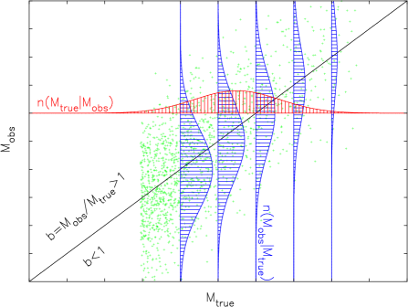
Figure 1: A toy-model example of the excess up-scattering mass bias. Suppose one estimates weak lensing masses ($M_{\rm obs}$) of clusters of galaxies whose mass function decreases with increasing true mass ($M_{\rm true}$). The green dot symbols are an illustrative example of a distribution of clusters in $M_{\rm true}$–$M_{\rm obs}$ plane. Suppose errors in observed weak lensing masses are symmetric, the number counts of clusters with a fixed $M_{\rm true}$ (or in a narrow $M_{\rm true}$–bin) as a function of $M_{\rm obs}$ would look like $n(M_{\rm obs}|M_{\rm true})$ shown as blue vertical hatched distributions. Due to the decreasing mass function, the number counts of clusters with a fixed $M_{\rm obs}$ (or in a narrow $M_{\rm obs}$–bin) as a function of $M_{\rm true}$, $n(M_{\rm true}|M_{\rm obs})$, is not symmetric about $M_{\rm true}=M_{\rm obs}$, but would look like one shown as a red horizontal hatched distribution (note that this distribution can be skewed in actual cases). It can be seen from it that the peak or mean of the distribution is located at a lower side of $M_{\rm true}=M_{\rm obs}$, which schematically explains the mechanism of the excess up-scattering mass bias.

Here we first give a briefly overview of the standard method of estimating cluster mass, and then describe a mechanism of the bias arising in that process. Commonly the standard $\chi^{2}$ analysis is adopted to estimate individual cluster mass with the following procedure: A tangential shear profile, $\gamma_{t}(\theta)$, (or converting it into the surface mass density, $\Delta\Sigma(R)$, see equation (1)) is measured, and its theoretical model with a few model parameters (commonly, the cluster mass, $M$, and the concentration parameter, $c$) is ready. Then, along with covariance matrix in which appropriate noise components are included, the $\chi^{2}$ distribution is computed, and is used to derive point estimators (commonly the best likelihood point is taken) and confidence intervals of model parameters. Therefore, in short, a set of model parameters that, in a statistical sense, best reproduces a measured noisy shear profile is taken as the best-fitting model. It is indeed random noises in the measured shear profile combined with a non-flat cluster mass function that induces the bias by the mechanism described below (see also Figure 1 for a toy-model example): A measured shear profile can be up-/down-scattered by positive/negative noise, which may lead to over-/under-estimation of the derived best-fitting weak lensing mass (which we denote as $M_{\rm obs}$). Consider a cluster with an observed weak lensing mass of $M_{\rm obs}^{*}$, its true cluster mass, $M_{\rm true}^{*}$, can be either $M_{\rm true}^{*}<M_{\rm obs}^{*}$ or $M_{\rm true}^{*}>M_{\rm obs}^{*}$ depending on a noise realization. Since the cluster mass function is a decreasing function with increasing mass, it is more likely that $M_{\rm obs}^{*}$ is the result of up-scattering of smaller $M_{\rm true}^{*}$ than that of down-scattering of larger $M_{\rm true}^{*}$. Defining the mass bias parameter as $b=M_{\rm obs}/M_{\rm true}$, and considering a sample of clusters with observed weak lensing mass of $M_{\rm obs}^{*}$, the above argument leads to an expectation that the averaged $b$ over the sample is $\langle b\rangle>1$. This is also the case for a sample of clusters with observed weak lensing mass greater than $M_{\rm obs}^{*}$. We call this bias “excess up-scattering mass bias”.

The excess up-scattering mass bias is conceptually closely related to the Eddington bias, which is known to have mainly two effects on weak lensing cluster studies; the one is the mass bias described in the last paragraph, and the other is the excess number counts of weak lensing shear-selected clusters which are found as high peaks in weak lensing mass maps (Hamana et al., 2004, 2012; Miyazaki et al., 2018). The latter is caused by an excess up-scattering effect on weak lensing peak signals in weak lensing mass maps reconstructed from noisy shear data; since weak lensing peak counts is a decreasing function with increasing peak-height, for a given observed weak lensing peak with its height $\nu^{*}$, it is more likely that the $\nu^{*}$-peak is the result of up-scattering of intrinsically (meaning an imaginary pure weak lensing signal without noise) lower $\nu_{\rm int}^{*}(<\nu^{*})$-peak than that of down-scattering of intrinsically higher $\nu_{\rm int}^{*}(>\nu^{*})$-peak. Chen et al. (2020) examined Eddington bias on the weak lensing mass estimate of weak lensing shear-selected clusters paying special attention to the fact that weak lensing cluster finding and following mass estimate use the same weak lensing shear data and thus both the processes are affected by the up-scattering effect. They quantified the mass biases for different cluster redshifts using a large sample of realistic mock weak lensing clusters for a deep weak lensing survey with a source galaxy number density of 30 arcmin^-2. Ramos-Ceja et al. (2022) studied X-ray properties of the shear-selected clusters of Oguri et al. (2021), in which the mass bias values derived in Chen et al. (2020) were used to correct the mass bias on the weak lensing cluster masses.

Recently, a weak lensing cluster search becomes a practical tool to construct a large sample of clusters of galaxies thanks to dedicated wide field surveys, for example, currently the largest sample is 187 shear-selected clusters from the Hyper Suprime-Cam survey S19A data by Oguri et al. (2021). In the near future, the size of shear-selected sample will become much larger as many more wide-area weak lensing-oriented surveys will come; in particular, the Legacy Survey of Space and Time (LSST, Ivezić et al., 2019) and Euclid survey (Laureijs et al., 2012; Racca et al., 2018) will cover a large portion of the sky with a sufficient depth. It is thus worth developing methods for correcting the mass bias on weak lensing mass estimate for shear-selected cluster samples without relying on mock simulations of realistic weak lensing clusters. This is exactly the purpose of this paper.

In this paper, we present an empirical method for correcting the excess up-scattering mass bias on weak lensing mass estimate for shear-selected cluster samples. In doing this, we adopt the framework of the standard Bayesian statistics along with the standard weak lensing cluster mass estimate scheme, and we use recent models of properties of dark matter halos under the cold dark matter structure formation scenario for a prior knowledge of weak lensing clusters. We test the method using mock simulations of weak lensing clusters.

The structure of this paper is as follows: In Section 2, we summarize basic theory of cluster weak lensing and halo models of clusters of galaxies which are used in weak lensing cluster mass estimate and to develop an empirical method for correcting the excess up-scattering mass bias. In Section 3, we describe a mock simulation of weak lensing clusters which is used to examine excess up-scattering mass bias, and to test its correction method. Methods of weak lensing analyses of mock clusters and a method for correcting the excess up-scattering mass bias are described in Section 4. Results of those analyses are presented in Section 5. In Section 6, we apply our correction method to the weak lensing shear-selected cluster sample of Hamana et al. (2020), and present the bias corrected masses. Finally, we summarize and discuss our results in Section 7.

2 Basics and models of cluster weak lensing

Here we summarize the basic theory of cluster weak lensing and halo models of clusters of galaxies which are used in weak lensing cluster mass estimate and to develop an empirical method for correcting the excess up-scattering mass bias on the weak lensing mass estimate in section 4.3.

2.1 Basics of cluster weak lensing

The central quantity of cluster weak lensing is the tangential component of the lensing shear at a source galaxy position $\bm{\theta_{s}}$ relative to a cluster center $\bm{\theta_{\rm cl}}$, $\gamma_{t}(\bm{\theta_{s}}:\bm{\theta_{\rm cl}})$. This is, however, a noisy quantity for individual source galaxy; for example, the amplitude of lensing shear from a cluster of our interest ($M\gtsim 10^{14}M_{\odot}/h$ at $0.1\ltsim z\ltsim 0.8$) at the cluster scale radius is $\sim 0.1$, but the root-mean-square of intrinsic galaxy shape noise is $\sim 0.3$ per component. Therefore, an optimal statistical estimator derived by an averaging operation which efficiently extracts the cluster lensing signal while reducing noise is employed according to a science case.

For the cluster mass estimate, the most commonly used estimator is the azimuthally averaged tangential shear profile which relates to the excess surface mass density, $\Delta\Sigma$, as (Kaiser et al., 1995),

$$\gamma_{t}(R)={{\bar{\Sigma}(<R)-\Sigma(R)}\over{\Sigma_{\rm cr}(z_{\rm cl},z_{\rm s})}}\equiv{{\Delta\Sigma(R)}\over{\Sigma_{\rm cr}(z_{\rm cl},z_{\rm s})}},$$ (1)

where $\Sigma(R)$ and $\bar{\Sigma}(<R)$ are the azimuthally averaged surface mass density at $R$ and interior to $R$, respectively, and the reciprocal critical surface mass density is calculated as

$$\Sigma_{\rm cr}^{-1}(z_{\rm cl},z_{\rm s})=\left\{\begin{array}[]{ll}0&\mbox{if $z_{\rm s}\leq z_{\rm cl}$,}\\ {{4\pi G}\over{c^{2}}}{{D_{l}D_{ls}}\over{D_{s}}}&\mbox{otherwise,}\end{array}\right.$$ (4)

where $D_{l}$, $D_{s}$ and $D_{ls}$ are the angular diameter distances between an observer and a lens, between an observer and a lens, and between a lens and a source, respectively.

For weak lensing cluster search, high peaks in a weak lensing mass map, which is the convergence field ($\kappa$) convolved with a kernel function ($U$), are searched for as strong candidates of massive clusters. A weak lensing mass map is evaluated from the tangential shear data (Schneider, 1996),

$${\cal{K}}(\bm{\theta}) = \int d^{2}\bm{\phi}~{}\kappa(\bm{\phi}-\bm{\theta})U(|\bm{\phi}|)$$ (5)

$$= \int d^{2}\bm{\phi}~{}\gamma_{t}(\bm{\phi}:\bm{\theta})Q(|\bm{\phi}|),$$

where the filter function $Q$ is related to $U$ by,

$$Q(\theta)={2\over\theta^{2}}\int_{0}^{\theta}d\theta^{\prime}\theta^{\prime}U(\theta^{\prime})-U(\theta).$$ (6)

The truncated Gaussian kernel for $U$ is widely adopted (Miyazaki et al., 2002a; Hamana et al., 2015), its $Q$ filter is

$$Q(\theta)={1\over{\pi\theta^{2}}}\left[1-\left(1+{{\theta^{2}}\over{\theta_{G}^{2}}}\right)\exp\left(-{{\theta^{2}}\over{\theta_{G}^{2}}}\right)\right],$$ (7)

for $\theta<\theta_{o}$ and $Q=0$ elsewhere. For filter parameters, we take $\theta_{G}=1.5$ arcmin and $\theta_{o}=15$ arcmin that were adopted in the weak lensing cluster finding by Hamana et al. (2020). The variance of noises on mass maps coming from the intrinsic galaxy shapes (which we call the shape noise) is evaluated by (Schneider, 1996)

$$\sigma_{\rm shape}^{2}={\sigma_{e}^{2}\over{2n_{g}}}\int d\theta\theta Q^{2}(\theta),$$ (8)

where $\sigma_{e}$ is the root-mean-square value of intrinsic ellipticity of galaxies and $n_{g}$ is the number density of source galaxies.

2.2 Halo models of clusters of galaxies

For the model of the matter density profile of clusters of galaxies, we adopt the truncated NFW model (Navarro et al., 1997; Baltz et al., 2009), which is known to reproduce the averaged tangential shear profile of dark matter halos measured from simulations of gravitational lensing ray-tracing through cosmological dark matter distributions (Oguri & Hamana, 2011) well. The NFW model is characterized by two parameters, the characteristic density ($\rho_{S}$) and the scale radius ($r_{s}$) or equivalently the halo mass and the concentration parameter. To define those quantities, we take the conventional over-density parameter ($\Delta$) relative to the critical density, $M_{\Delta}\equiv 4\pi r_{\Delta}^{3}\Delta\rho_{cr}(z)/3=M_{\rm NFW}(<r_{\Delta})$. The corresponding concentration parameter is given by $c_{\Delta}=r_{\Delta}/r_{s}$. For choices of the over-density, we take $\Delta=200$ and 500, and denote the corresponding mass as $M_{200c}$ and $M_{500c}$, respectively.

For the halo mass function, we adopt a model by Tinker et al. (2010). For the model of a probability distribution of the concentration parameter, we take the log-normal model,

$$P(c|M)={1\over{\sqrt{2\pi}\sigma_{\ln c}}}\exp\left(-{{\left[\ln c-\ln\bar{c}(M)\right]^{2}}\over{2\sigma_{\ln c}^{2}}}\right){1\over c},$$ (9)

where $\bar{c}(M)$ the mean mass-concentration relation for which we adopt a model by Diemer & Joyce (2019), and we adopt $\sigma_{\ln c}=0.25$ following Chen et al. (2020).

2.3 Projection effect by large-scale structures

In addition to weak lensing signals from a target cluster of galaxies, other lensing signals come from large-scale structures along the same line-of-sight, which is called the projection effect. In order to include this effect into mock weak lensing clusters, we use full-sky gravitational lensing simulation data from Takahashi et al. (2017). They performed gravitational lensing ray-tracing simulations using the multiple-lens spherical plane algorithm through a nested system of cubic $N$-body simulation boxes of different sizes (Shirasaki et al., 2015), which enables a full-sky gravitational lensing simulation with a high angular resolution of $\theta_{\rm eff}<1$ arcmin. Lensing shear and convergence data are computed at grid points of the HEALPix pixelization with $N_{\rm side}=8192$ (corresponding to an effective pixel scale of 0.43 arcmin, Górski et al. (2005)) on 38 source planes located at equal intervals of the comoving 150 $h^{-1}$Mpc from $z=0.05$ to $z=5.34$. 108 realizations of a full-sky lensing data set along with dark matter halo catalog in the corresponding $N$-body boxes were generated.

In the full-sky simulation data, there are regions affected by lensing of massive halos. In order to avoid a chance overlap between them and our mock cluster, we exclude regions within 10 arcmin from halos with $M_{200c}\geq 3\times 10^{14}M_{\odot}h^{-1}$, and within 5 arcmin from halos with $8\times 10^{13}\leq M_{200c}<3\times 10^{14}M_{\odot}h^{-1}$. About 50 percent of the total area is excluded by these conditions.

3 Mock simulations of cluster weak lensing

Here we describe mock simulations of weak lensing clusters which are used to examine the excess up-scattering mass bias in weak lensing mass estimates and to test our method for correcting it. In designing the mock simulation, we adopt observational parameters of Hamana et al. (2020) as we apply our bias correction method to their weak lensing shear-selected cluster sample in Section 6.

3.1 Setting of the mock simulation

Here we describe the setting of the mock simulation of a weak lensing cluster observation.

3.1.1 Cosmological model

We adopt the WMAP cosmology (Hinshaw et al., 2013) as it was adopted in the full-sky gravitational lensing simulations by Takahashi et al. (2017) which we use to extract lensing shear signals from large-scale structures in the same line-of-sights of mock clusters (see Sections 2.3 and 3.2).

3.1.2 Redshift distribution of source galaxies

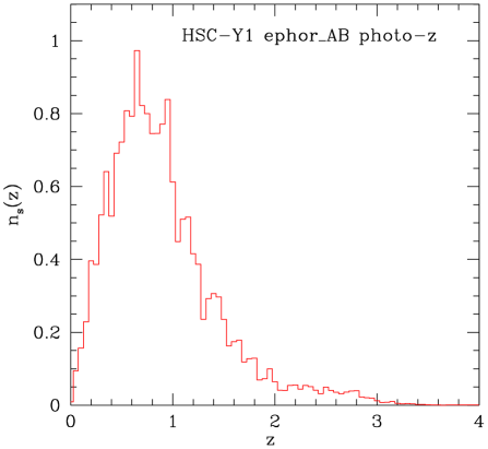
Figure 2: An estimate of redshift distribution of the source galaxy sample used in a weak lensing cluster search by Hamana et al. (2020), which is adopted in simulations of mock weak lensing clusters in this study. The distribution is computed by summing up the redshift probability distributions, which are derived in photo-$z$ estimation for each galaxy, over selected source galaxies. The normalization is taken so that $\int dzn_{s}(z)=1$

We adopt the redshift distribution of source galaxies estimated by Hamana et al. (2020) shown in Figure 2. In short, they performed a weak lensing cluster search using the Hyper SuprimeCam survey first-year (HSC-Y1) weak lensing shape catalog (Mandelbaum et al., 2018), to which photometric redshift (photo-$z$) information derived using HSC five-band photometry (Tanaka et al., 2018) is linked. They adopted Ephor_AB photo-$z$ data among six photo-$z$ methods applied to the HSC-Y1 galaxy catalog (Tanaka et al., 2018), and selected source galaxies using the photo-$z$ information with the $P$-cut method (Oguri, 2014). The redshift distribution of selected galaxies shown in Figure 2 is estimated by summing the full probability distribution functions of redshift, $P(z)$, derived in photo-$z$ estimations taking into account the lensing weight $w$; $n_{s}(z)=\sum_{i}w_{i}P_{i}(z)/\sum_{i}w_{i}$, where the summation is taken over all the selected galaxies. The effective number density of selected galaxies was $n_{g}=19.3$ arcmin^-2.

3.2 The recipe for mock weak lensing clusters

We generate samples of mock weak lensing clusters for four cluster redshifts, $z_{\rm cl}=0.15$, 0.25, 0.35, and 0.45. Each mock cluster and associated source galaxies are generated by the following procedure:

(1) Random choices of a true cluster mass and concentration: We consider the range of the cluster mass $1\times 10^{13}<M_{200c}<2\times 10^{15}M_{\odot}h^{-1}$, and randomly choose a true mass (which we denote $M_{\rm true}$) according to the halo mass function by Tinker et al. (2010). Then, we randomly choose a concentration parameter according to the log-normal probability distribution, equation (9).

(2) Adding a perturbation to the cluster mass to take account of complexities of cluster mass distribution: Mass distributions of clusters do not exactly follow the NFW profile, but deviate from it due to, for example, the triaxiality and existence of substructures (Oguri et al., 2005; Corless & King, 2007; Meneghetti et al., 2010; Becker & Kravtsov, 2011; Oguri & Hamana, 2011; Bahé et al., 2012). In order to include effects of these deviations into mock weak lensing clusters, we follow a prescription by Chen et al. (2020); that is, we adopt a statistical relation between a realistic halo with a true mass $M_{\rm true}$ and an NFW halo with a mass $M_{\rm NFW}$ whose tangential shear profile best describes that of the realistic halo, $P(M_{\rm NFW}|M_{\rm true})$. Based on the findings by Becker & Kravtsov (2011), and Bahé et al. (2012), Chen et al. (2020) modeled $P(M_{\rm NFW}|M_{\rm true})$ by a log-normal distribution,

$$M_{\rm NFW}=M_{\rm true}\exp(\Delta_{\rm NFW}),$$ (10)

where $\Delta_{\rm NFW}$ is the normal distribution with the standard deviation of $\sigma_{\rm NFW}$. Chen et al. (2020) took $\sigma_{\rm NFW}=0.18$ which we adopt in this work, which approximately corresponds to a 20 percent scatter in mass. Thus, for each mock cluster with $M_{\rm true}$, we draw an $M_{\rm NFW}$ according to equation (10), and use it to model the lensing shear profile later in step (4).

(3) Placing source galaxies in the sky and redshift-space: Source galaxies are randomly placed around a cluster with the mean number density of $n_{g}=20$ arcmin^-2, and a redshift of each galaxy is assigned randomly according to the redshift probability distribution of Hamana et al. (2020) shown in Figure 2 (see section 3.1.2 for details). The redshift range is limited to $0<z<5.34$ because of the availability of the full-sky gravitational lensing simulation data (see Section 2.3),

(4) Assigning shear signals and noise to each galaxy: Having set the model parameters of a cluster and positions and redshift of the source galaxies, we assign weak lensing shear signals and a noise to each galaxy. We take into account the following three components: Lensing shear signals from the cluster ($\gamma_{\rm cl}$) and from large-scale structures in the same line-of-sight of each source galaxy ($\gamma_{\rm lss}$, see section 2.3), and a noise due to intrinsic galaxy shape ($n_{\rm shape}$). We describe them in turn as follows:

1. Cluster component: We adopt the truncated NFW model (see section 2.2) for which the analytical expressions of the lensing signals are given in the literature (e.g., Baltz et al., 2009). Therefore, for each source galaxy with given redshift and perpendicular distance from a cluster center, the cluster shear component, $\gamma_{\rm cl}$, is calculated using the analytical expressions.

2. Large-scale structure component: We use full-sky gravitational lensing simulation data by Takahashi et al. (2017) (see section 2.3 for its brief description) to assign $\gamma_{\rm lss}$ to each galaxy: First, for each cluster, we randomly choose its position in a simulation sky, and then the sky position of every source galaxy is automatically determined and the simulation pixel containing it is as well. Then for each source galaxy, we extract simulation shear data from the corresponding pixel on the source plane which is closest to the galaxy redshift and assign it to that galaxy.

3. Noise component: For each galaxy, we draw an intrinsic shape noise $n_{\rm shape}$ according to the normal distribution with the standard deviation of $\sigma_{\gamma,{\rm int}}=0.4$.

For each cluster redshift, we generate 10,000 clusters per one full-sky simulation data set. We used all the 108 available data sets, and thus we have 1,080,000 clusters for each cluster redshift.

4 Methods of weak lensing analyses and a mass bias correction

Having prepared the mock weak lensing shear catalog for each cluster, we first perform two weak lensing analyses, a measurement of weak lensing peak height in a mass map, and a standard weak lensing cluster mass estimate using a tangential shear profile. We then test our empirical method for mitigating the excess up-scattering mass bias on the weak lensing mass estimate for shear-selected cluster samples. In this section, we describe methods for these analyses.

4.1 The peak height in a weak lensing mass map

The peak height of a cluster in a weak lensing mass map is computed by a discrete form of equation (5),

$${\cal{K}}={1\over{n_{g}}}\sum_{i}\gamma_{t,i}Q(|\bm{\phi}_{i}|),$$ (11)

where the summation is taken over all galaxies within $\theta_{o}$ from a cluster center, and the filter function $Q$ is given by equation (7). We evaluate the shape noise $\sigma_{\rm shape}^{2}$ using equation (8) with $n_{g}=20$arcmin^-2 and $\sigma_{e}=0.4$. We define the signal-to-noise ratio of the peak height as

$$SN_{\rm peak}={\cal{K}}/\sigma_{\rm sharp}.$$ (12)

In addition to this noisy estimator, we also compute $SN_{\rm NFW}$ which is a peak signal solely from the NFW cluster shear (by replacing $\gamma_{t}=\gamma_{t,{\rm cl}}+\gamma_{t,{\rm lss}}+n_{t,{\rm shape}}$ in equation (11) with $\gamma_{t,{\rm cl}}$) normalized by the same $\sigma_{\rm shape}$.

4.2 Standard weak lensing cluster mass estimate

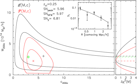
Figure 3: Example of mock tangential shear profile and results of $\chi^{2}$-fit of model parameters. Results of a mock cluster of $z_{\rm cl}=0.25$ are shown. In the inserted panel, points show bin-averaged tangential shear profile ($\gamma_{t}(R_{i})$) with error bars showing diagonal components of covariance matrix ($\sqrt{\rm Cov}_{ii}$). The solid line shows the best fit model. The left panel show contour maps (68% and 95% confidence levels) of the likelihood (black) and posterior (red) functions with best-fitting positions being marked by the plus and cross, respectively. The green plus in a circle shows the input model parameters. The right-hand panel shows the marginalized one-dimensional probability functions of the cluster mass in the form of $\Delta\chi^{2}(M)=-2\log{\cal{L}}(M)/{\cal{L}}_{\rm best}$. Dashed lines show the true mass and best-fitting masses shown in the left-hand panel.

In short, we derive a cluster mass by first computing the radial bin-averaged tangential shear profile for each cluster, and then fitting it to the NFW model profile based on the standard $\chi^{2}$ likelihood analysis. Below we describe those steps in more details (see Miyatake et al., 2019; Umetsu et al., 2020, and references therein for further details).

We compute a bin-averaged tangential shear profile in five radial bins of equal logarithmic spacing of $\Delta\log R=0.25$ with bin centers of $R_{c}(i)=0.3\times 10^{i\Delta\log R}$ [$h^{-1}$Mpc], where $i$ runs from 0 to 4. In order to avoid the dilution effect by foreground and/or cluster member galaxies (Broadhurst et al., 2005; Limousin et al., 2007; Hoekstra, 2007; Medezinski et al., 2018; Umetsu & Broadhurst, 2008; Okabe et al., 2010), we use only galaxies that are well behind a target cluster, to be specific, $z>z_{\rm cl}+0.05$.

We employ standard likelihood analysis for deriving constraints on model parameters. The log-likelihood is given by

$$-2\ln{\cal{L}}(\bm{p})=\sum_{i,j}[d_{i}-m_{i}(\bm{p})]{\rm Cov}_{ij}^{-1}[d_{j}-m_{j}(\bm{p})],$$ (13)

where the data vector $d_{i}=\gamma_{t}(R_{i})$, and $m_{i}(\bm{p})$ is the model prediction with the model parameters $\bm{p}=(M_{200c},c_{200c})$. We adopt the truncated NFW model (see Section 2.2) for the lens model, whereas deviations from it due to, e.g., triaxiality and existence of substructures, are taken into account in the covariance (see below). In computing the source redshift weighted tangential shear profile of the truncated NFW model, we use the redshift distribution of source galaxies for each cluster. The covariance matrix (Cov) is composed of the three components, (see Umetsu et al., 2020, and references therein for detailed descriptions): The statistical uncertainties due to the galaxy intrinsic shape noise (Cov^shape); the cosmic shear covariance due to the projection effect of uncorrelated large-scale structures (Cov^lss, see for details Hoekstra, 2003); and the intrinsic variance of the cluster lensing signal due to, e.g., triaxiality of clusters and presence of substructures (Cov^int, see for details Gruen et al., 2015; Miyatake et al., 2019).

We compute the log-likelihood function over the two-parameter space in the range of $5\times 10^{12}<M_{200c}<3\times 10^{15}M_{\odot}h^{-1}$, and $0.1<c_{200c}<30$. We adopt the maximum point of the likelihood function as the best-fitting model, and denote its mass as $M_{L}$. In order to derive confidence intervals of $M_{200c}$, we marginalize over $c_{200c}$ in the range $1<c_{200c}<30$ with $1/c_{200c}$ weight (or a log-uniform prior for $c_{200c}$), because it is appropriate to assume a log-uniform prior, instead of a uniform prior, for a positive-definite quantity (Umetsu et al., 2020), and the lower-bound of $c_{200c}>1$ is taken as a physically reasonable choice.

In order to define the signal-to-noise ratio of hte measured tangential shear profile, we employ the standard quadratic estimator,

$$SN_{\gamma}^{2}=\sum_{i}\left[\gamma_{t}(R_{i})/{\rm Cov}_{ii}^{\rm shape}\right]^{2},$$ (14)

where the summation is taken over all the bins with $\gamma_{t}(R_{i})>0$.

For the pirpose of illustration, we present one example of weak lensing analyses of a mock cluster in Figure 3. Shown is a case with $M_{\rm true}\simeq 3\times 10^{14}M_{\odot}h^{-1}$ (in $M_{200c}$) and $z_{\rm cl}=0.25$. As one can see in the plot, for most individual clusters, the concentration parameter is not well constrained due to a limited $R$ range. Also it is unlikely that estimated concentration parameters are affected by a systematic bias like the excess up-scattering mass bias, because, unlike the halo mass function, the probability distribution of the concentration parameter is not a monotonic function. Therefore, in this paper we do not deal with constraints on the concentration parameter.

4.3 An empirical method for mitigating the excess up-scattering mass bias

In developing a method, we have set the following two requirements: (1) It should not rely on simulations of mock weak lensing clusters, but should be based on analytical or empirical models of dark matter halos of cluster scale. (2) It can be directly incorporated into the standard weak lensing cluster mass estimation scheme.

For the framework of our correction method, we employ the standard Bayesian statistics written in conventional notation as follows:

$$P(M,c|\gamma_{t}^{obs})\propto L(\gamma_{t}^{obs}|M,c)Pr(M,c),$$ (15)

where $P$, $L$, and $Pr$ are the posterior probability, the likelihood function, and the prior, respectively, with model parameters $(M,c)$ and an observed shear profile ($\gamma_{t}^{obs}$).

A natural choice of the likelihood function is ${\cal{L}}(M,c)$ defined in equation (13). For the prior of the cluster mass and concentration parameter, we employ empirical models of their probability distributions from recent numerical simulations of structure formation; the mass function of dark matter halos, $n(M)$, by Tinker et al. (2010), and the log-normal probability distribution of the concentration parameter, equation (9), with the mean mass–concentration relation by Diemer & Joyce (2019), thus we have

$$Pr(M,c)=\left\{\begin{array}[]{ll}n(M)P(c|M)&\mbox{for $SN_{\gamma}^{\rm NFW}(M,c)>1$,}\\ 0&\mbox{otherwise,}\end{array}\right.$$ (18)

where $SN_{\gamma}^{\rm NFW}(M,c)$ is the signal-to-noise ratio of shear profile of NFW models defined in the same manner as in equation (14) but using a model prediction of the shear profile. The condition of $SN_{\gamma}^{\rm NFW}(M,c)>1$ is imposed to avoid the prior increasing monotonically toward lower mass, which results in a non-physical upturn of the posterior at a very low-mass range. The choice of threshold is arbitrary, but it needs to include all the reasonably possible parameter space. We empirically take the threshold of $SN_{\gamma}^{\rm NFW}>1$ considering our selection of $SN_{\rm peak}>5$.

4.4 Note on different $SN$s

In this study, we use different $SN$s, namely, $SN_{\rm peak}$ (defined by equation (12)), $SN_{\rm NFW}$ (introduced in section 4.1), $SN_{\gamma}$ (defined by equation (14)), and $SN_{\gamma}^{\rm NFW}$ (introduced in section 4.3). Here we clarify the differences between them.

$SN_{\rm peak}$ and $SN_{\gamma}$ are actual observables, and are strongly correlated with each other because those $SN$s come from the same lensing shear signals of a cluster, although different angular weights (the kernel function $Q$ for a weak lensing mass map, and an angular scale of $\gamma_{t}$ measurement) cause scatter between them. In addition, in actual measurement processes, there is another factor that may cause a systematic difference between them. It is different selections of source galaxies used in each measurement: In weak lensing peak search, the redshifts of clusters are unknown in advance, and thus a galaxy sample used to generate a mass map is commonly selected by a simple magnitude cut on a single photometry band (for example Miyazaki et al., 2002b; Hamana et al., 2015). Such a galaxy sample inevitably contains foreground and cluster member galaxies, which results in the dilution effect on the peak heights and thus on $SN_{\rm peak}$ (Hamana et al., 2020). Once a peak is matched with a known cluster with redshift information, a sample of background galaxies can be selected by multi-band photometric information (see Medezinski et al., 2018, and references therein), which is used to estimate a weak lensing cluster mass with the $\gamma_{t}$ profile. Therefore $SN_{\gamma}$ is less affected by the dilution effect.

$SN_{\rm NFW}$ and $SN_{\gamma}^{\rm NFW}$ are defined in the same manner as $SN_{\rm peak}$ and $SN_{\gamma}$, respectively, but their signal levels are computed assuming a pure NFW model without taking any noise component into account. Thus, those $SN$s are model predictions of corresponding peak and $\gamma_{t}$ measurements for a cluster with a set of model parameters.

5 Results

In this section, we present results of weak lensing analyses of mock clusters. We first present results of standard weak lensing analyses (described in sections 4.1 and 4.2) focusing on the excess up-scattering mass bias. Then, we test the method for correcting the bias described in section 4.3.

5.1 Results of standard weak lensing analyses of mock clusters

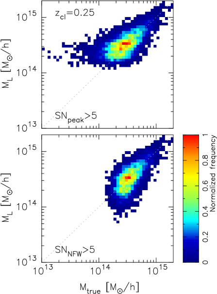
Figure 4: Frequency distributions of weak lensing clusters in the $M_{\rm true}$–$M_{L}$ (in $M_{200c}$) plane. The top-panel is for clusters selected with the noisy weak lensing peak height of $SN_{\rm peak}>5$, whereas the bottom-panel is for clusters selected with the peak height only from the NFW component of $SN_{\rm NFW}>5$. The results from the mock cluster sample of $z_{\rm cl}=0.25$ are shown.

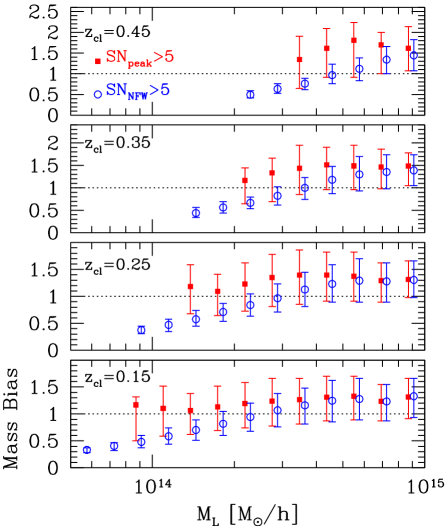
Figure 5: Mass biases, defined by $b=M_{L}/M_{\rm true}$, as a function of $M_{L}$ (in $M_{200c}$) is shown. Symbols show the average values of mock cluster samples in $M_{L}$-bins, and error bars show the 16th and 84th percentiles of the samples in each bin. Filled squares are for clusters selected with the noisy weak lensing peak height of $SN_{\rm peak}>5$, whereas open circles are for clusters selected with the peak height only from the NFW component of $SN_{\rm NFW}>5$. Note that the results are slightly shifted in the horizontal direction for clarity.

Figure 4 shows frequency distributions of weak lensing clusters in the $M_{\rm true}$–$M_{L}$ plane. The top-panel is for clusters selected with the noisy weak lensing peak height of $SN_{\rm peak}>5$ (namely, shear-selected clusters), whereas the bottom-panel is for clusters selected with the peak height from the NFW component only, $SN_{\rm NFW}>5$. In the bottom panel, there is a cut-off at $M_{\rm true}\sim 1\times 10^{14}M_{\odot}h^{-1}$ which is due to a tight correlation between $M_{\rm true}$ at a fixed $z_{\rm cl}$ and $SN_{\rm NFW}$ combined with the $SN_{\rm NFW}$ threshold. In the top panel, no such cut-off is seen, but the distribution spreads toward lower $M_{\rm true}$, which is due to the Eddington bias studied in detail by Chen et al. (2020); in short, some fraction of clusters with $SN_{\rm NFW}$ values below the selection threshold are up-scattered by noises and pass the selection threshold of $SN_{\rm peak}>5$. The tangential shear profiles of such clusters are also most likely up-scattered, because the same weak lensing shear data are used in both the peak height measurement and the weak lensing mass estimate. Therefore, as a result, for such up-scattered clusters, $M_{L}$ is systematically larger than $M_{\rm true}$. This is quantitatively shown in Figure 5, where the mass bias defined by

$$b={{M_{L}}\over{M_{\rm true}}},$$ (19)

is plotted as a function of $M_{L}$, with symbols showing the average values of mock cluster samples in $M_{L}$-bins, and error bars showing the 16th and 84th percentiles of the binned samples. It is seen in the figure that for the sample with $SN_{\rm peak}>5$ selection, the average values of biases are greater than unity; to be specific $\langle b\rangle\sim 1.1-1.8$ depending on $M_{L}$ and the redshift.

Another important point seen in Figure 5 is that even for the sample selected by $SN_{\rm NFW}>5$, the average values of biases are greater than unity at high-$M_{L}$ ranges. Since there is no Eddington bias effect on this $SN_{\rm NFW}$-selected sample, this is purely the result of the excess up-scattering mass bias. This indicates that the excess up-scattering mass bias is not a phenomenon unique to shear-selected samples but can also present in cluster samples selected by other methods. Notice that at lower $M_{L}$ ranges, the biases decline as decreasing $M_{L}$. This is a selection effect caused by the low-$M_{\rm true}$ cut-off seen in the bottom-panel of Figure 4, and because of this, only down-scattered clusters can enter lower-$M_{L}$ bins, resulting in $b<1$.

It is important to note that although the best-fitting masses are, on average, biased high, the marginalized one-dimensional likelihood distributions of the mass give a statistically correct confidence intervals. In fact, it is found from results of mock weak lensing cluster analyses of shear-selected sample ($SN_{\rm peak}>5$) that in 72(96) percent of samples, $M_{\rm true}$ is within a conventional 1(2)-$\sigma$ confidence interval of the marginalized distribution (to be more specific, $M_{\rm true}$ is within the range of $\Delta\chi^{2}(M)<1(4)$). This indeed suggests that the weak lensing mass estimate scheme itself is correctly working, but the probability of up- and down-scattering is not symmetric, causing the biased best-fitting masses, on average.

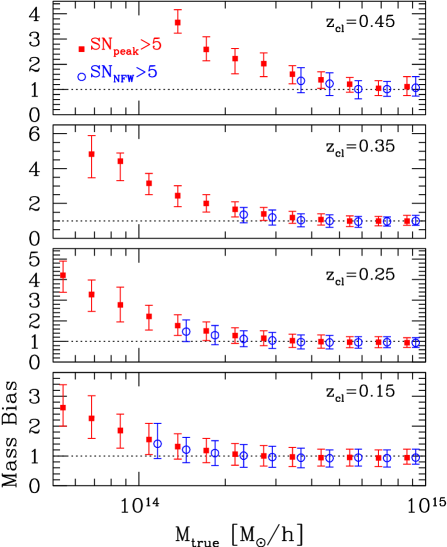
Figure 6: Same as Figure 5 but mass biases as a function of $M_{\rm true}$ (in $M_{200c}$) is shown. To be specific, the mass biases are computed for mock cluster samples in $M_{\rm true}$-bins.

Next, we look into the mass bias as a function of $M_{\rm true}$, because, although it is not a direct observable, it may give some insight into the excess up-scattering mass bias. Figure 6 shows the mass bias computed for mock cluster samples in $M_{\rm true}$-bins. At lower $M_{\rm true}$ ranges, the bias for the $SN_{\rm peak}>5$ selection increases as decreasing $M_{\rm true}$, which is due to the Eddington bias effect seen in the top-panel of Figure 4. The bias for $SN_{\rm NFW}>5$ selection also shows a similar trend which is due to a selection effect as is seen in the bottom-panel of Figure 4. At higher $M_{\rm true}$ ranges, averaged biases are very close to unity. This is a natural consequence of nearly unbiased noise properties of tangential shears, leading to nearly unbiased scattering of $M_{L}$ for a sample of clusters within a narrow $M_{\rm true}$-bin. It should be emphasized that the excess up-scattering mass bias does not arise solely from up- and down-scattering due to unbiased noises, but arises from scatterings over a wide mass range combined with a non-flat cluster mass function. Therefore, an averaged bias of a sample of clusters in a narrow $M_{\rm true}$ range is not affected by the excess up-scattering effect, because non-symmetric scatterings do not occur in that sample. However, when one infers the true mass of a weak lensing cluster from a wide range of potential true masses (or a mass range where a likelihood, ${\cal L}(M)$, is non-negligible), one needs to take into account the non-symmetric scattering effect and thus needs to take into account the shape of the mass function (or the prior information in the Bayesian framework). This is a basic concept of our method for correcting the excess up-scattering mass bias.

5.2 Testing the bias correction method with mock weak lensing clusters

We test our method for mitigating the excess up-scattering mass bias with the mock weak lensing clusters. For each mock cluster, we compute the posterior distribution defined in equation (15) with the likelihood function, equation (13), and the prior, equation (18). We take the maximum point of the posterior distribution as the best-fitting model, and denote its mass as $M_{P}$.

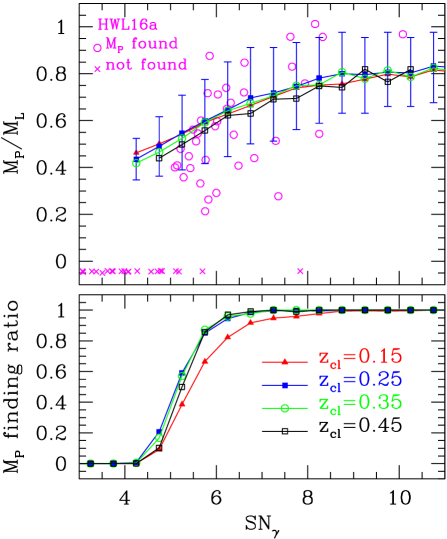
Figure 7: Bottom panel: The $M_{P}$ finding ratios as a function of $SN_{\gamma}$ evaluated using mock cluster samples are shown. Different symbols with different colors are for mock cluster samples with different redshift $z_{\rm cl}$. Top panel: Statistics of $M_{P}/M_{L}$ ($M_{200c}$) are shown as a function of $SN_{\gamma}$. Symbols with error bars (plotted only for $z_{\rm cl}=0.25$, for clarity) show the average values and the 16th and 84th percentiles of mock cluster samples in $SN_{\gamma}$-bins. Magenta symbols show $M_{P}/M_{L}$ for individual clusters of HWL16a sample (Hamana et al., 2020): open circles and crosses (placed at $M_{P}/M_{L}=-0.05$) are for clusters with $M_{P}$ found, and not found, respectively

An example of the posterior distribution is shown in Figure 3 as red contours. It is seen in the plot that the posterior is truncated at a low-mass side that is due to the cutoff imposed on the prior, $Pr=0$ for $SN_{\gamma}^{\rm NFW}<1$, see equation (18). The marginalized one-dimensional posterior of $M$ is truncated at a low-mass side as well. Due to this truncation, there are cases in which the maximum and peak point (not at the low-mass edge of the posterior distribution) of the posterior distribution does not exist, and thus $M_{P}$ is not determined. We evaluate ratios of cases that do have $M_{P}$ for all the cases as a function of $SN_{\gamma}$ and present the result in the bottom panel of Figure 7. It is seen in the Figure that the ratio drops at $SN_{\gamma}\sim 6$ and below, and is zero below $SN_{\gamma}\sim 4$. The reason for this is that the smaller $SN_{\gamma}$ is, the broader the likelihood function becomes, with its maximum point being generally at smaller mass, resulting in its posterior being more affected by the truncation of the prior. This makes the limitations of our correction method evident; for our method to be workable, a high signal-to-noise ratio measurement of $SN_{\gamma}\gtsim 5$ is required.

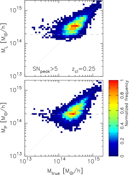
Figure 8: Frequency distributions of mock weak lensing clusters selected with $SN_{\rm peak}>5$ in $M_{\rm true}$–$M_{L}$ plane (top panel) and $M_{\rm true}$–$M_{P}$ plane (bottom panel). All the cluster masses are in $M_{200c}$. Note in both the panels, a sample of mock clusters with $M_{P}$ found is used. The results from the mock sample of $z_{\rm cl}=0.25$ are shown. The horizontal dashed line in each panel shows the empirical mass scale $M_{s}$ obtained by the condition, equation (20).

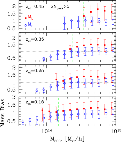
Figure 9: Mass biases defined either by $b=M_{L}/M_{\rm true}$ as a function of $M_{L}$ (red filled squares) or by $b=M_{P}/M_{\rm true}$ as a function of $M_{P}$ (blue open circles) are shown. All the cluster masses are in $M_{200c}$. Symbols show the average values of mock cluster samples in $M$-bins, and error bars show the 16th and 84th percentiles of the samples in each bin. A sample of mock clusters selected with $SN_{\rm peak}>5$ is used. Note that the results are slightly shifted in the horizontal direction for clarity. The vertical dashed line in each panel shows the empirical mass scale $M_{S}$, below which the bias values are affected by the cluster selection (see main text in Section 5.2 for details).

Next, we examine the performance of our correction method. The frequency distribution of mock weak lensing clusters selected with $SN_{\rm peak}>5$ in the $M_{\rm true}$–$M_{P}$ plane is shown in the bottom panel of Figure 8, and the distribution of the same sample but in $M_{\rm true}$–$M_{L}$ plane is shown in the top panel. Comparing the two plots, one can see a trend that the distribution moves to down as a result of the correction. The mass bias after the correction, defined by $b=M_{P}/M_{\rm true}$, as a function of $M_{P}$ is shown by open circles with error bars in Figure 8. In that plot, a trend that the bias decreases at lower-mass ranges is seen. This is a consequence of sample selection with $SN_{\rm peak}$; to be more specific, only clusters with $M_{P}<M_{\rm true}$ exist at a lower-$M_{P}$ range (see Figure 8). We empirically define a mass scale (denoted by $M_{s}$), below which the averaged bias is affected by the sample selection, by introducing the following condition,

$$\int dcP(c|M_{s})SN_{\rm NFW}(M_{s},c)=4,$$ (20)

where $SN_{\rm NFW}$ is the model prediction of the weak lensing peak height defined in the same manner as $SN_{\rm peak}$, equation (12). The derived mass scales are shown in Figure 9 as vertical dashed lines, and in Figure 8 as horizontal dashed lines. It is seen from Figure 9 that in the mass range $M_{P}>M_{s}$, our correction method works well, with resulting bin averaged mass biases being close to unity within $\sim 10$ percent.

Finally, we check if the marginalized one-dimensional posterior distributions of the mass give proper credible intervals of the true mass. Since the posterior distribution is truncated at the low-mass side, the marginalized 1D posterior is truncated as well. Taking the case shown in Figure 3 as an example, as can be seen in the right-hand panel, the conventional 1-$\sigma$ credible interval is safely determined, but the 2-$\sigma$ interval is not. It is found that in 74(38) percent of all the mock clusters that do have $M_{P}$, the 1(2)-$\sigma$ credible interval of 1D posterior distribution is determined. Then, it is found that in 66(95) percent of the cases with the 1(2)-$\sigma$ credible interval being determined, $M_{\rm true}$ is within the 1(2)-$\sigma$ credible interval of the 1D posterior distribution. Therefore, we may conclude that if credible intervals are determined, the marginalized 1D posterior distributions of the mass give proper credible intervals of the true mass.

6 Application to HWL16a sample

We apply our correction method of the excess up-scattering mass bias to the weak lensing shear-selected cluster sample of Hamana et al. (2020) (which we call “HWL16a sample”). They conducted weak lensing cluster search using Hyper Suprime-Cam Subaru Strategic Program (HSC survey) first-year data (Aihara et al., 2018b, a). They searched for high peaks in weak lensing mass maps covering an effective area of $\sim 120$ deg² generated using HSC survey first-year weak lensing shape catalog (Mandelbaum et al., 2018). They found 124 high peaks with $SN_{\rm peak}>5$, and cross-matched them with the public optical cluster catalog (CAMIRA, Oguri et al., 2018) constructed from the same HSC survey data to identify cluster counter-parts of the peaks. They defined the sub-sample of 64 secure clusters, and performed weak lensing mass estimate for 61 clusters located at $z_{\rm cl}<0.7$ among the 64 clusters.

The weak lensing mass estimation method of Hamana et al. (2020) is basically identical with one adopted in our mock weak lensing cluster analysis described in Section 4 (in fact, our method is based on theirs) except for their use of photo-$z$ probability distribution functions to select background source galaxies and to evaluate $\Sigma_{\rm cr}^{-1}$ (see for details Appendix 3 of Hamana et al., 2020, and reference therein). Its impact on mass estimate was studies in Miyatake et al. (2019); Umetsu et al. (2020), they found that the induced uncertainty in estimated mass is less than 2 percent which is much smaller than the statistical uncertainty. Therefore, we directly apply our correction method, equation (15), with the prior, equation (18), to HWL16a secure clusters with likelihood functions derived in Hamana et al. (2020). In so doing, we adopt the cosmological model from Planck 2018 result (Planck Collaboration et al., 2020), and we consider two cases, $\Delta=200$ and $\Delta=500$.

lcclrcccc Results of the weak lensing mass estimate for HWL16a sample are summarized. Columns 6–7 are for the over-density parameter relative to the critical density of $\Delta=200$, and Columns 8–9 are for $\Delta=500$. $M_{L}$ and $M_{P}$ are the estimated cluster mass before and after the correction for the excess up-scattering mass bias is applied, respectively. Errors are taken from the 1-$\sigma$ confidence interval of marginalized 1D probability distributions. ”N/A” means that a corresponding value is not obtained. RA Dec $M_{200c}[10^{14}M_{\odot}h^{-1}]$ $M_{500c}[10^{14}M_{\odot}h^{-1}]$
ID J2000.0[^∘] $z_{\rm cl}$ $SN_{\gamma}$ $M_{L}$ $M_{P}$ $M_{L}$ $M_{P}$
HWL16a-002 30.4273 $-5.0219$ 0.234 6.62 $3.35_{-1.35}^{+1.08}$ $2.84_{-1.05}^{+1.08}$ $2.51_{-0.93}^{+0.60}$ $1.93_{-0.74}^{+0.79}$
HWL16a-003 31.2073 $-3.0587$ 0.553 2.72 $2.57_{-1.51}^{+1.53}$ N/A $1.95_{-1.14}^{+0.86}$ N/A
HWL16a-005 31.4584 $-3.3714$ 0.167 3.51 $0.99_{-0.35}^{+0.78}$ N/A $0.83_{-0.33}^{+0.53}$ N/A
HWL16a-007 33.1112 $-5.6214$ 0.287 7.36 $7.69_{-4.22}^{+0.65}$ $2.13_{-1.24}^{+1.29}$ $2.98_{-1.20}^{+1.04}$ $1.48_{-0.87}^{+0.91}$
HWL16a-012 35.4434 $-3.7668$ 0.430 6.02 $5.39_{-2.64}^{+2.45}$ $3.22_{-1.45}^{+1.48}$ $3.71_{-1.63}^{+0.93}$ $2.22_{-1.03}^{+1.06}$
HWL16a-013 36.1229 $-4.2378$ 0.264 5.56 $2.62_{-1.37}^{+1.05}$ $1.34_{-0.98}^{+0.93}$ $1.80_{-0.86}^{+0.45}$ $0.87_{-{\rm N/A}}^{+0.68}$
HWL16a-014 36.3758 $-4.2496$ 0.155 5.65 $2.41_{-1.41}^{+0.98}$ $0.80_{-{\rm N/A}}^{+0.92}$ $1.56_{-0.83}^{+0.41}$ N/A
HWL16a-016 37.3963 $-3.6121$ 0.312 6.83 $6.09_{-2.72}^{+1.73}$ $2.68_{-1.18}^{+1.23}$ $3.35_{-1.38}^{+0.75}$ $1.85_{-0.82}^{+0.86}$
HWL16a-017 37.5572 $-5.6526$ 0.500 3.08 $4.06_{-3.02}^{+1.27}$ N/A $2.16_{-1.44}^{+0.72}$ N/A
HWL16a-020 37.9163 $-4.8799$ 0.186 10.08 $5.04_{-1.72}^{+1.44}$ $4.88_{-1.25}^{+1.26}$ $3.78_{-1.16}^{+0.84}$ $3.43_{-0.90}^{+0.89}$
HWL16a-022 38.1580 $-4.7513$ 0.276 5.98 $2.88_{-1.40}^{+1.10}$ $1.66_{-1.02}^{+1.04}$ $2.05_{-0.92}^{+0.52}$ $1.10_{-0.78}^{+0.76}$
HWL16a-023 38.3915 $-5.5027$ 0.420 4.07 $1.99_{-0.78}^{+1.08}$ N/A $1.60_{-0.66}^{+0.65}$ N/A
HWL16a-024 129.3206 $1.6069$ 0.360 3.74 $3.26_{-1.93}^{+1.34}$ N/A $2.19_{-1.21}^{+0.68}$ N/A
HWL16a-026 130.5895 $1.6473$ 0.424 6.48 $11.77_{-4.51}^{+3.63}$ $4.80_{-2.01}^{+1.98}$ $6.54_{-2.35}^{+1.34}$ $3.33_{-1.37}^{+1.37}$
HWL16a-028 133.1296 $0.4041$ 0.270 6.23 $3.66_{-1.68}^{+1.44}$ $2.38_{-1.06}^{+1.10}$ $2.54_{-1.08}^{+0.68}$ $1.61_{-0.75}^{+0.79}$
HWL16a-032 138.4612 $-0.7631$ 0.285 5.67 $3.58_{-1.70}^{+1.36}$ $2.15_{-1.07}^{+1.11}$ $2.46_{-1.08}^{+0.65}$ $1.44_{-0.76}^{+0.80}$
HWL16a-034 139.0387 $-0.3966$ 0.315 7.94 $9.16_{-2.77}^{+2.71}$ $6.95_{-1.91}^{+1.86}$ $6.32_{-1.74}^{+1.37}$ $4.85_{-1.32}^{+1.30}$
HWL16a-035 139.3198 $0.9985$ 0.344 3.93 $2.93_{-2.02}^{+1.05}$ N/A $1.28_{-0.79}^{+0.75}$ N/A
HWL16a-036 139.3405 $3.8281$ 0.420 5.22 $3.94_{-1.93}^{+1.58}$ $1.89_{-{\rm N/A}}^{+1.38}$ $2.75_{-1.27}^{+0.81}$ $1.23_{-{\rm N/A}}^{+1.01}$
HWL16a-037 140.0954 $1.5748$ 0.697 2.98 $13.48_{-10.51}^{+3.97}$ N/A $6.98_{-5.01}^{+1.67}$ N/A
HWL16a-038 140.1431 $0.7907$ 0.463 3.09 $1.51_{-0.64}^{+1.67}$ N/A $1.27_{-0.59}^{+1.04}$ N/A
HWL16a-039 140.4154 $-0.2491$ 0.310 5.18 $2.52_{-1.53}^{+1.16}$ N/A $1.70_{-0.96}^{+0.46}$ N/A
HWL16a-041 140.6790 $2.1327$ 0.194 5.28 $2.82_{-1.65}^{+1.17}$ $1.01_{-{\rm N/A}}^{+1.04}$ $1.85_{-0.97}^{+0.43}$ $0.58_{-{\rm N/A}}^{+0.81}$
HWL16a-045 177.2946 $0.3636$ 0.260 4.08 $2.40_{-1.82}^{+0.27}$ N/A $0.99_{-0.57}^{+0.47}$ N/A
HWL16a-046 177.5842 $-0.6009$ 0.135 6.22 $2.00_{-0.83}^{+0.80}$ $1.48_{-0.79}^{+0.86}$ $1.53_{-0.61}^{+0.45}$ $0.96_{-0.59}^{+0.64}$
HWL16a-047 178.0615 $0.5187$ 0.472 5.81 $4.03_{-0.87}^{+1.70}$ $2.89_{-{\rm N/A}}^{+1.91}$ $3.38_{-0.84}^{+1.09}$ $1.88_{-{\rm N/A}}^{+1.41}$
HWL16a-050 178.8288 $0.8712$ 0.481 3.73 $4.48_{-3.19}^{+1.35}$ N/A $1.76_{-1.21}^{+1.02}$ N/A
HWL16a-051 179.0517 $-0.3490$ 0.254 8.25 $7.10_{-2.63}^{+2.10}$ $3.86_{-1.33}^{+1.37}$ $4.07_{-1.37}^{+0.88}$ $2.63_{-0.90}^{+0.94}$
HWL16a-052 179.6138 $-0.0412$ 0.252 4.72 $2.91_{-2.06}^{+0.53}$ N/A $1.41_{-0.80}^{+0.44}$ N/A
HWL16a-053 180.4286 $-0.1839$ 0.167 7.30 $3.68_{-2.07}^{+1.70}$ $1.89_{-1.00}^{+1.09}$ $2.44_{-1.23}^{+0.53}$ $1.29_{-0.73}^{+0.78}$
HWL16a-056 181.3878 $-0.6432$ 0.470 4.81 $4.82_{-2.47}^{+1.83}$ N/A $2.98_{-1.42}^{+0.95}$ N/A
HWL16a-057 210.7874 $-0.3084$ 0.450 4.27 $5.79_{-3.28}^{+2.19}$ N/A $3.40_{-1.80}^{+1.00}$ N/A
HWL16a-058 211.2955 $-0.1472$ 0.248 5.10 $3.07_{-1.62}^{+1.10}$ $1.23_{-{\rm N/A}}^{+1.13}$ $2.02_{-0.96}^{+0.54}$ $0.77_{-{\rm N/A}}^{+0.84}$
HWL16a-059 211.7872 $-0.2717$ 0.561 3.28 $2.83_{-2.05}^{+1.53}$ N/A $1.95_{-1.37}^{+1.02}$ N/A
HWL16a-060 211.9925 $-0.4857$ 0.469 5.83 $8.97_{-4.11}^{+2.57}$ $2.36_{-{\rm N/A}}^{+2.05}$ $4.70_{-1.90}^{+1.35}$ $1.63_{-{\rm N/A}}^{+1.44}$
HWL16a-064 213.7770 $-0.4892$ 0.144 7.84 $5.65_{-3.99}^{+0.10}$ N/A $1.87_{-1.02}^{+0.76}$ N/A
HWL16a-070 215.2574 $0.3665$ 0.645 4.78 $10.58_{-5.63}^{+3.77}$ N/A $5.54_{-2.76}^{+1.67}$ N/A
HWL16a-071 215.9165 $0.4491$ 0.534 3.99 $5.25_{-3.12}^{+1.82}$ N/A $2.97_{-1.56}^{+0.95}$ N/A
HWL16a-076 216.7785 $0.7267$ 0.296 8.33 $3.26_{-1.39}^{+1.38}$ $3.12_{-0.97}^{+1.00}$ $2.51_{-0.98}^{+0.73}$ $2.18_{-0.70}^{+0.72}$
HWL16a-077 216.8310 $0.9541$ 0.294 5.49 $2.42_{-1.07}^{+0.87}$ $1.36_{-{\rm N/A}}^{+1.03}$ $1.80_{-0.76}^{+0.48}$ $0.87_{-{\rm N/A}}^{+0.74}$
HWL16a-080 217.6808 $0.8093$ 0.312 6.60 $5.04_{-2.19}^{+1.92}$ $3.63_{-1.32}^{+1.35}$ $3.55_{-1.37}^{+0.86}$ $2.50_{-0.93}^{+0.97}$
HWL16a-081 218.8457 $-0.3931$ 0.283 6.03 $1.49_{-0.28}^{+0.77}$ $1.06_{-{\rm N/A}}^{+0.91}$ $1.24_{-0.27}^{+0.56}$ $0.57_{-{\rm N/A}}^{+0.72}$
HWL16a-084 220.0846 $-0.6101$ 0.549 3.62 $6.35_{-4.62}^{+1.30}$ N/A $2.56_{-1.62}^{+1.24}$ N/A
HWL16a-088 220.7952 $1.0452$ 0.528 3.72 $4.97_{-2.97}^{+2.52}$ N/A $3.49_{-1.97}^{+1.11}$ N/A
HWL16a-090 221.1442 $0.2464$ 0.295 5.14 $3.18_{-1.77}^{+1.22}$ $1.30_{-{\rm N/A}}^{+1.11}$ $2.09_{-1.04}^{+0.50}$ $0.85_{-{\rm N/A}}^{+0.81}$
HWL16a-091 221.1917 $-0.6694$ 0.523 5.77 $9.83_{-4.50}^{+3.86}$ $4.25_{-2.00}^{+2.00}$ $6.01_{-2.54}^{+1.29}$ $2.93_{-1.40}^{+1.44}$
HWL16a-093 221.3335 $0.1116$ 0.286 6.38 $3.74_{-1.70}^{+1.30}$ $2.02_{-1.00}^{+1.05}$ $2.39_{-1.02}^{+0.62}$ $1.36_{-0.70}^{+0.74}$
HWL16a-094 223.0801 $0.1689$ 0.592 5.76 $25.86_{-11.72}^{+N/A}$ $5.52_{-3.88}^{+3.07}$ $13.70_{-6.07}^{+1.42}$ $3.89_{-2.68}^{+2.27}$
HWL16a-095 223.0929 $-0.9713$ 0.304 7.66 $5.42_{-1.89}^{+1.68}$ $4.50_{-1.33}^{+1.33}$ $3.89_{-1.24}^{+0.92}$ $3.13_{-0.94}^{+0.94}$
HWL16a-097 224.2746 $0.1164$ 0.220 4.57 $2.18_{-1.33}^{+0.78}$ N/A $1.45_{-0.81}^{+0.37}$ N/A
HWL16a-098 224.6567 $0.4858$ 0.395 5.12 $5.17_{-3.35}^{+0.93}$ N/A $2.46_{-1.29}^{+0.67}$ N/A
HWL16a-101 245.3758 $42.7648$ 0.152 8.16 $3.23_{-1.06}^{+0.94}$ $3.27_{-1.04}^{+1.08}$ $2.54_{-0.80}^{+0.58}$ $2.26_{-0.76}^{+0.79}$
HWL16a-102 246.1339 $43.3203$ 0.287 5.70 $3.61_{-1.94}^{+1.24}$ N/A $1.93_{-0.98}^{+0.63}$ N/A
HWL16a-103 246.5173 $43.7147$ 0.260 5.59 $1.98_{-0.78}^{+0.71}$ $1.08_{-{\rm N/A}}^{+0.94}$ $1.52_{-0.60}^{+0.45}$ $0.61_{-{\rm N/A}}^{+0.71}$
HWL16a-104 333.0522 $-0.1334$ 0.350 6.00 $6.79_{-3.26}^{+1.49}$ $1.98_{-1.32}^{+1.28}$ $3.20_{-1.32}^{+0.86}$ $1.36_{-0.95}^{+0.89}$
HWL16a-107 333.5929 $0.7956$ 0.308 5.40 $3.73_{-1.82}^{+1.38}$ $1.67_{-1.17}^{+1.11}$ $2.33_{-1.07}^{+0.66}$ $1.11_{-{\rm N/A}}^{+0.79}$
HWL16a-110 335.2140 $0.9704$ 0.323 5.43 $5.06_{-2.26}^{+1.78}$ $2.01_{-{\rm N/A}}^{+1.34}$ $2.98_{-1.26}^{+0.87}$ $1.36_{-{\rm N/A}}^{+0.95}$
HWL16a-112 336.0366 $0.3331$ 0.154 7.62 $3.30_{-1.16}^{+0.99}$ $3.16_{-1.05}^{+1.09}$ $2.56_{-0.85}^{+0.59}$ $2.17_{-0.76}^{+0.80}$
HWL16a-114 336.4066 $-0.3068$ 0.402 3.37 $2.30_{-1.36}^{+1.07}$ N/A $1.63_{-0.92}^{+0.52}$ N/A
HWL16a-115 336.4217 $1.0730$ 0.281 5.86 $2.59_{-0.76}^{+0.99}$ $2.27_{-1.05}^{+1.11}$ $2.10_{-0.64}^{+0.61}$ $1.52_{-0.76}^{+0.81}$
HWL16a-117 337.1293 $1.7135$ 0.338 6.32 $5.87_{-2.50}^{+2.26}$ $3.97_{-1.49}^{+1.52}$ $4.06_{-1.56}^{+1.01}$ $2.75_{-1.05}^{+1.08}$

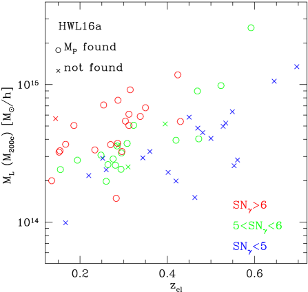
Figure 10: Distribution of the HWL16a weak lensing cluster sample in $M_{L}$–$z_{\rm cl}$ plane. The weak lensing masses, $M_{L}$, are re-derived adopting the maximum point of the likelihood function, ${\cal{L}}(M,c)$, as the best-fitting model (in the original study by Hamana et al. (2020), the peak of the marginalized 1D likelihood function was adopted as a point estimator of the weak lensing mass). The open circles are clusters with $M_{P}$ being found, whereas the crosses are ones with $M_{P}$ being not found. Different colors are for different ranges of cluster’s $SN_{\gamma}$ values, see colored labels in the plot.

The derived cluster masses are summarized in Table 6. We also evaluate the signal-to-noise ratio of the measured $\Delta\Sigma(R)$ profile with the corresponding shape noise covariance, and we summarize the obtained values in Table 6. Note that the resulting $SN$ is equivalent to $SN_{\gamma}$ (defined in equation (14)) evaluated for mock clusters because the tangential shear and $\Delta\Sigma(R)$ are related by equation (1), and thus we denote it by $SN_{\gamma}$.

The distribution of HWL16a clusters in the $z_{\rm cl}$–$M_{L}(M200c)$ plane is shown in Figure 10. $M_{P}$ is found for 37(36) out of the 61 clusters for $\Delta=200(500)$. In Figure 10, clusters with $M_{P}$ being found are shown by open circles, whereas ones without $M_{P}$ are shown by crosses, and different colors are for different ranges of cluster’s $SN_{\gamma}$ values. It is seen in the figure that clusters with lower-$SN_{\gamma}$, which are generally located at a high-$z_{\rm cl}$ and low-$M_{L}$ region, fail to obtain $M_{P}$. This tendency is also seen in the top panel of Figure 7. In that figure the distribution in the $SN_{\gamma}$–$M_{P}/M_{L}$ ($M_{200c}$) plane is shown, where clusters without $M_{P}$ are placed at $M_{P}/M_{L}=-0.05$. It is found from this figure that the results from the HWL16a sample are broadly consistent with results from mock clusters, especially in the following two points: (1) For the HWL16a sample, the $M_{P}$ finding ratio drops at below $SN_{\gamma}\sim 6$, and no HWL16a cluster with $M_{P}$ successfully found exists at $SN_{\gamma}<5$. This trend is very similar to that of mock clusters. (2) The overall trend of $M_{P}/M_{L}$ as a function of $SN_{\gamma}$ for individual HWL16a cluster is in line with the trend seen in mock clusters. Finally, we evaluate the mean value of the $M_{P}/M_{L}$ ratios among HWL16a clusters that do have $M_{P}$, and we obtain $\langle M_{P}/M_{L}\rangle=0.58$ with ${\rm RMS}=0.21$ (for $M_{200c}$).

7 Summary and discussions

We have examined the excess up-scattering mass bias on the weak lensing mass estimate for shear-selected cluster samples, and have present the empirical method for mitigating it.

We have generated samples of realistic mock weak lensing clusters for four redshifts ($z_{\rm cl}=0.15$, 0.25, 0.35 and 0.45) taking into account the following three components (see Section 3.2); the cluster lensing including deviations from the NFW profile, lensing contributions from large-scale structures, and the noise component from intrinsic galaxy shapes. We have performed the standard weak lensing mass estimate for the shear-selected ($SN_{\rm peak}>5$) mock clusters, and found the mass-bin averaged mass bias is in the range of $1.1-1.8$ depending on cluster mass and the redshift. Another important finding from the mock weak lensing analyses is that even before the correction for the excess up-scattering mass bias is applied, the marginalized one-dimensional probability distributions of the mass for individual clusters give statistically correct confidence intervals. We thus emphasize that the standard weak lensing mass estimation method itself is working correctly, but the probability of up- and down-scattering is not symmetric, resulting in the biased best-fitting masses, on average.

Our correction method uses the framework of the standard Bayesian statistics with the likelihood function from weak lensing mass estimate based on the standard $\chi^{2}$ analysis, and the prior of the probability distribution of the cluster mass and concentration parameter from recent empirical models (see Section 4.3). We tested our correction method with mock weak lensing clusters. It was found that our correction method works well, with resulting mass-bin averaged mass biases being close to unity within $\sim 10$ percent.

However, our method has limitations that a high signal-to-noise ratio measurement of $SN_{\gamma}\gtsim 5$ is required for the method to work properly. This is due to the artificial truncation of the prior on a low-mass side, which is imposed to avoid a non-physical upturn of the posterior at a very low-mass range. A possible cause of the non-physical upturn is a combination of the following two factors: One is the fact that the likelihood function changes only slowly on the lower-mass side, because the model shear profile approaches $\gamma_{t}(\theta)\rightarrow 0$ as the mass decreases. The other is the power-law shape of halo mass function on a lower-mass range with a negative power-law index. One possible way to resolve the non-physical upturn is to modify the prior so that it includes a condition that clusters are shear-selected; that is, the probability that a cluster appears as a high peak in a weak lensing mass map decreases as the cluster mass decreases. We, however, leave such modifications of the method for a future study.

We applied the method to the HWL16a weak lensing shear-selected cluster sample, and derived bias corrected weak lensing cluster masses (summarized in Table 6). Because of the limitations of our method, the bias corrected masses, $M_{P}$, were obtained only for clusters with a high signal-to-noise ratio of $SN_{\gamma}\gtsim 5$. In 61 HWL16a clusters, $M_{P}$ is found for 37(36) clusters for $\Delta=200(500)$, among which we found the mean value of the $M_{P}/M_{L}$ to be $\langle M_{P}/M_{L}\rangle=0.58$ with ${\rm RMS}=0.21$ (for $M_{200c}$).

Before closing this paper, we comment on a proper use of the bias corrected mass, $M_{P}$: As is demonstrated in Figure 1, the excess up-scattering mass bias arises when one considers the probability of $M_{\rm true}$ for a given $M_{L}$, $P(M_{\rm true}|M_{L})$, but does not arise when one considers $P(M_{L}|M_{\rm true})$ (here we assume the error in a weak lensing mass estimate is symmetric and there are no other systematic or selection effects on a cluster sample). It is also important to note that $P(M_{P}|M_{\rm true})$ is a biased distribution in the sense that it gives $\langle M_{P}\rangle=\int dM_{P}M_{P}P(M_{P}|M_{\rm true})<M_{\rm true}$. One simple example of a proper use of $M_{P}$ is to suppose one has a shear-selected cluster sample, and tries to divide clusters into some sub-samples so that their mean masses equal to true masses. In this case, one should make sub-samples with $M_{P}$, in other words, one should divide clusters into $M_{P}$–bins. Then an expectation value of $M_{\rm true}$ of a sub-samples in a narrow $M_{P}$–bins is $M_{\rm true}\simeq M_{P}$. The other simple example in which one should not use $M_{P}$ is if one has a cluster sample selected by a good tracer of the true mass (denoted by $X$), and estimates a mean true mass of a sub-sample of clusters in a narrow $X$–bin. In this case, one should not use $M_{P}$ but use $M_{L}$, because $P(M_{L}|X)\sim P(M_{L}|M_{\rm true})$ is the unbiased probability distribution which gives $\langle M_{L}\rangle\simeq M_{\rm true}$ (see a discussion in the last paragraph of section 5.1). We note that in actual recent studies on deriving cluster scaling relations, for example one between X-ray temperatures and cluster masses, advanced methods such as Bayesian hierarchical models and Bayesian population modeling are adopted, in which scatters in measured quantities, including weak lensing mass, and the selection functions are statistically accounted for (Miyatake et al., 2019; Sereno et al., 2020; Umetsu et al., 2020; Akino et al., 2022; Chiu et al., 2022). Therefore, in such a study, one should not use $M_{P}$ to avoid double-counting of the excess up-scattering effect.

We would like to thank the anonymous referee for constructive comments on the earlier manuscript which improved the paper. We thank M. Oguri and K. Umetsu for useful discussions and comments. We would like to thank R. Takahashi for making full-sky gravitational lensing simulation data publicity available. The dark matter halo mass function and the mass-concentration relation used in this work were computed by routines wrapped up in Colossus (Diemer, 2018), we would like to thank B. Diemer for making it publicly available. We would like to thank Nick Kaiser for making the software imcat publicly available, we have heavily used it in this work. We would like to thank HSC data analysis software team for their effort to develop data processing software suite, and HSC data archive team for their effort to build and to maintain the HSC data archive system.

This work was supported in part by JSPS KAKENHI Grant Number JP22K03655.

Data analysis were in part carried out on the analysis servers at Center for Computational Astrophysics, National Astronomical Observatory of Japan. Numerical computations were in part carried out on Cray XC30 and XC50 at Center for Computational Astrophysics, National Astronomical Observatory of Japan, and also on Cray XC40 at YITP in Kyoto University.

This paper is partly based on data collected at the Subaru Telescope and retrieved from the HSC data archive system, which is operated by Subaru Telescope and Astronomy Data Center (ADC) at NAOJ. Data analysis was in part carried out with the cooperation of Center for Computational Astrophysics (CfCA) at NAOJ. We are honored and grateful for the opportunity of observing the Universe from Maunakea, which has the cultural, historical and natural significance in Hawaii.

References

- Aihara et al. (2018a) Aihara, H., Armstrong, R., Bickerton, S., et al. 2018a, PASJ, 70, S8
- Aihara et al. (2018b) Aihara, H., Arimoto, N., Armstrong, R., et al. 2018b, PASJ, 70, S4
- Akino et al. (2022) Akino, D., Eckert, D., Okabe, N., et al. 2022, PASJ, 74, 175
- Allen et al. (2011) Allen, S. W., Evrard, A. E., & Mantz, A. B. 2011, ARA&A, 49, 409
- Bahé et al. (2012) Bahé, Y. M., McCarthy, I. G., & King, L. J. 2012, MNRAS, 421, 1073
- Baltz et al. (2009) Baltz, E. A., Marshall, P., & Oguri, M. 2009, J. Cosmology Astropart. Phys, 1, 15
- Becker & Kravtsov (2011) Becker, M. R., & Kravtsov, A. V. 2011, ApJ, 740, 25
- Broadhurst et al. (2005) Broadhurst, T., Takada, M., Umetsu, K., et al. 2005, ApJ, 619, L143
- Chen et al. (2020) Chen, K.-F., Oguri, M., Lin, Y.-T., & Miyazaki, S. 2020, ApJ, 891, 139
- Chiu et al. (2022) Chiu, I. N., Ghirardini, V., Liu, A., et al. 2022, A&A, 661, A11
- Corless & King (2007) Corless, V. L., & King, L. J. 2007, MNRAS, 380, 149
- Diemer (2018) Diemer, B. 2018, ApJS, 239, 35
- Diemer & Joyce (2019) Diemer, B., & Joyce, M. 2019, ApJ, 871, 168
- Górski et al. (2005) Górski, K. M., Hivon, E., Banday, A. J., et al. 2005, ApJ, 622, 759
- Gruen et al. (2015) Gruen, D., Seitz, S., Becker, M. R., Friedrich, O., & Mana, A. 2015, MNRAS, 449, 4264
- Hamana et al. (2012) Hamana, T., Oguri, M., Shirasaki, M., & Sato, M. 2012, MNRAS, 425, 2287
- Hamana et al. (2015) Hamana, T., Sakurai, J., Koike, M., & Miller, L. 2015, PASJ, 67, 34
- Hamana et al. (2020) Hamana, T., Shirasaki, M., & Lin, Y.-T. 2020, PASJ, 72, 78
- Hamana et al. (2004) Hamana, T., Takada, M., & Yoshida, N. 2004, MNRAS, 350, 893
- Hinshaw et al. (2013) Hinshaw, G., Larson, D., Komatsu, E., et al. 2013, ApJS, 208, 19
- Hoekstra (2003) Hoekstra, H. 2003, MNRAS, 339, 1155
- Hoekstra (2007) —. 2007, MNRAS, 379, 317
- Ivezić et al. (2019) Ivezić, Ž., Kahn, S. M., Tyson, J. A., et al. 2019, ApJ, 873, 111
- Kaiser et al. (1995) Kaiser, N., Squires, G., & Broadhurst, T. 1995, ApJ, 449, 460
- Kravtsov & Borgani (2012) Kravtsov, A. V., & Borgani, S. 2012, ARA&A, 50, 353
- Laureijs et al. (2012) Laureijs, R., Gondoin, P., Duvet, L., et al. 2012, Society of Photo-Optical Instrumentation Engineers (SPIE) Conference Series, Vol. 8442, Euclid: ESA’s mission to map the geometry of the dark universe, 84420T
- Limousin et al. (2007) Limousin, M., Richard, J., Jullo, E., et al. 2007, ApJ, 668, 643
- Mandelbaum et al. (2018) Mandelbaum, R., Miyatake, H., Hamana, T., et al. 2018, PASJ, 70, S25
- Medezinski et al. (2018) Medezinski, E., Oguri, M., Nishizawa, A. J., et al. 2018, PASJ, 70, 30
- Meneghetti et al. (2010) Meneghetti, M., Rasia, E., Merten, J., et al. 2010, A&A, 514, A93
- Miyatake et al. (2019) Miyatake, H., Battaglia, N., Hilton, M., et al. 2019, ApJ, 875, 63
- Miyazaki et al. (2002a) Miyazaki, S., Hamana, T., Shimasaku, K., et al. 2002a, ApJ, 580, L97
- Miyazaki et al. (2002b) Miyazaki, S., Komiyama, Y., Sekiguchi, M., et al. 2002b, PASJ, 54, 833
- Miyazaki et al. (2018) Miyazaki, S., Oguri, M., Hamana, T., et al. 2018, PASJ, 70, S27
- Navarro et al. (1997) Navarro, J. F., Frenk, C. S., & White, S. D. M. 1997, ApJ, 490, 493
- Oguri (2014) Oguri, M. 2014, MNRAS, 444, 147
- Oguri & Hamana (2011) Oguri, M., & Hamana, T. 2011, MNRAS, 414, 1851
- Oguri et al. (2005) Oguri, M., Takada, M., Umetsu, K., & Broadhurst, T. 2005, ApJ, 632, 841
- Oguri et al. (2018) Oguri, M., Lin, Y.-T., Lin, S.-C., et al. 2018, PASJ, 70, S20
- Oguri et al. (2021) Oguri, M., Miyazaki, S., Li, X., et al. 2021, PASJ, 73, 817
- Okabe et al. (2010) Okabe, N., Takada, M., Umetsu, K., Futamase, T., & Smith, G. P. 2010, PASJ, 62, 811
- Planck Collaboration et al. (2020) Planck Collaboration, Aghanim, N., Akrami, Y., et al. 2020, A&A, 641, A6
- Pratt et al. (2019) Pratt, G. W., Arnaud, M., Biviano, A., et al. 2019, Space Sci. Rev., 215, 25
- Racca et al. (2018) Racca, G., Laureijs, R., & Mellier, Y. 2018, in 42nd COSPAR Scientific Assembly, Vol. 42, E1.16–3–18
- Ramos-Ceja et al. (2022) Ramos-Ceja, M. E., Oguri, M., Miyazaki, S., et al. 2022, A&A, 661, A14
- Schneider (1996) Schneider, P. 1996, MNRAS, 283, 837
- Sereno et al. (2020) Sereno, M., Umetsu, K., Ettori, S., et al. 2020, MNRAS, 492, 4528
- Shirasaki et al. (2015) Shirasaki, M., Hamana, T., & Yoshida, N. 2015, MNRAS, 453, 3043
- Takahashi et al. (2017) Takahashi, R., Hamana, T., Shirasaki, M., et al. 2017, ApJ, 850, 24
- Tanaka et al. (2018) Tanaka, M., Coupon, J., Hsieh, B.-C., et al. 2018, PASJ, 70, S9
- Tinker et al. (2010) Tinker, J. L., Robertson, B. E., Kravtsov, A. V., et al. 2010, ApJ, 724, 878
- Umetsu (2020) Umetsu, K. 2020, A&A Rev., 28, 7
- Umetsu & Broadhurst (2008) Umetsu, K., & Broadhurst, T. 2008, ApJ, 684, 177
- Umetsu et al. (2020) Umetsu, K., Sereno, M., Lieu, M., et al. 2020, ApJ, 890, 148