Schwinger-Dyson truncations in the all-soft limit: a case study

Abstract

We study a special Schwinger-Dyson equation in the context of a pure SU(3) Yang-Mills theory, formulated in the background field method. Specifically, we consider the corresponding equation for the vertex that governs the interaction of two background gluons with a ghost-antighost pair. By virtue of the background gauge invariance, this vertex satisfies a naive Slavnov-Taylor identity, which is not deformed by the ghost sector of the theory. In the all-soft limit, where all momenta vanish, the form of this vertex may be obtained exactly from the corresponding Ward identity. This special result is subsequently reproduced at the level of the Schwinger-Dyson equation, by making extensive use of Taylor’s theorem and exploiting a plethora of key relations, particular to the background field method. This information permits the determination of the error associated with two distinct truncation schemes, where the potential advantage from employing lattice data for the ghost dressing function is quantitatively assessed.

I Introduction

The Schwinger-Dyson equations (SDEs) form an infinite tower of coupled non-linear integral equations that govern the dynamical evolution of all $n$-point Green’s (correlation) functions of a quantum field theory Dyson (1949); Schwinger (1951a, b). The SDEs are derived formally from the generating functional of the theory Rivers (1988); Itzykson and Zuber (1980), and constitute one of the few nonperturbative frameworks available in the continuum Roberts and Williams (1994); Alkofer and von Smekal (2001); Maris and Roberts (2003); Fischer (2006); Binosi and Papavassiliou (2009, 2008); Huber (2020a). Over the years they have been employed in the study of a wide array of physical phenomena, encompassing, among others, superconductivity Dorey and Mavromatos (1990, 1992); Lee and Herbut (2002); Popovici (2013), dynamical chiral symmetry breaking Aguilar et al. (2018a); Gao et al. (2021); Mitter et al. (2015); Aguilar and Papavassiliou (2011); Fischer and Alkofer (2003); Roberts and Williams (1994), and the emergence of mass in strongly coupled theories, such as pure Yang-Mills theories and Quantum Chromodynamics (QCD) Cornwall (1982); Aguilar et al. (2008, 2019a, 2013a, 2021a, 2022); Horak et al. (2022); Papavassiliou (2022).

Even though, in principle, the SDEs encode the complete dynamical information of all correlation functions of the theory, in practice their treatment requires the implementation of truncations. For instance, certain vertices or multi-particle kernels that enter in the diagrammatic representation of a given SDE may be set to their tree-level value, or be completely neglected. Similarly, dressed-loop approximations may be adopted, where only a given order of diagrams in a loop-wise expansion is retained. However, due the lack of a definite expansion parameter, there is no a-priori way of estimating the error committed due to such approximations. Instead, the errors may be estimated only a-posteriori, either by direct comparison with experimental results or lattice simulations, or, more laboriously, by introducing further structures, i.e., dressing vertices or adding loops, and computing their numerical impact. This is to be contrasted with approaches possessing an obvious expansion parameter, such as large $N_{c}$ ’t Hooft (1974); Witten (1979); Coleman (1985), or heavy mass ($M$) expansions Eichten and Hill (1990); Georgi (1990), where, at the $n$-th step, the neglected terms are of order ${\cal O}(1/N_{c}^{n+1})$ or ${\cal O}(1/M^{n+1})$.

It would be clearly instructive to consider a toy SDE scenario where the exact result for the Green’s function in question is known by virtue of general field-theoretic principles, and the numerical impact of certain typical truncations may be easily evaluated. To that end, we turn to the well-known framework of the Background Field Method (BFM) DeWitt (1967); Honerkamp (1972); Kallosh (1974); Kluberg-Stern and Zuber (1975); Arefeva et al. (1974); Abbott (1981); Weinberg (1980); Abbott (1982); Shore (1981); Abbott et al. (1983), where the gauge field $A_{\mu}$ is decomposed as $A_{\mu}=B_{\mu}+Q_{\mu}$, with $B_{\mu}$ the classical (background) part and $Q_{\mu}$ the quantum (fluctuating) component, and a special gauge-fixing procedure is employed. Within this formalism we derive and analyze the SDE of the four-particle vertex that consists of two background gluons and a ghost-antighost pair, to be denoted by ${\rm BB\bar{c}c}\,$. It is important to emphasize that, due to the background gauge symmetry, this vertex satisfies an Abelian Slavnov-Taylor identity (STI) when contracted by the momentum carried by any of its background legs. Note that Abelian STIs are direct generalizations of tree-level relations, and, in contradistinction to the STIs Taylor (1971); Slavnov (1972) of the linear covariant gauges Fujikawa et al. (1972), they receive no modifications from the ghost sector of the theory.

It turns out that it is possible to obtain an exact nontrivial result for the vertex ${\rm BB\bar{c}c}\,$by appealing directly to this latter STI, which relates the divergence of ${\rm BB\bar{c}c}\,$with the three-particle vertex $\rm B\overline{c}c$ Aguilar et al. (2018b) at different permutations of its arguments. As some of the momenta involved are set to zero, certain known limits of the vertex $\rm B\overline{c}c$ are triggered; and finally, in the all-soft limit, i.e., when all incoming momenta vanish, the STI becomes a Ward identity (WI) that expresses ${\rm BB\bar{c}c}\,$in terms of the ghost-dressing function at the origin. Past its formal simplicity, the main advantage of this results is that, in the Landau gauge, it fully determines the deep infrared structure of the vertex ${\rm BB\bar{c}c}\,$in terms of a quantity that has been extensively studied both on the lattice Sternbeck et al. (2005); Ilgenfritz et al. (2007); Cucchieri and Mendes (2007); Bogolubsky et al. (2007); Cucchieri and Mendes (2008, 2010); Bogolubsky et al. (2009); Maas (2013); Boucaud et al. (2012); Ayala et al. (2012); Boucaud et al. (2017, 2018) and in the continuum Aguilar et al. (2008); Boucaud et al. (2008); Fischer et al. (2009); Tissier and Wschebor (2010); Pennington and Wilson (2011); Vandersickel and Zwanziger (2012); Dudal et al. (2012); Aguilar et al. (2013b); Cyrol et al. (2018); Gao et al. (2018); Aguilar et al. (2019b); Corell et al. (2018); Huber (2020a); Aguilar et al. (2021b).

Evidently, when all incoming momenta are set to zero at the level of the SDE governing the ${\rm BB\bar{c}c}\,$, and in the absence of truncations or approximations, i.e., when the SDE is treated exactly, the above result must emerge identically. However, as we will elucidate in the main text, the correct implementation of the all-soft limit is rather subtle, hinging on fundamental properties of vertices and kernels entering in the diagrammatic expansion of the SDE under consideration. Once all field-theoretic principles have been correctly taken into account, one recovers precisely the same result at the level of the SDE as that obtained from the WI.

The above analysis is particularly instructive, because it exposes the delicate interplay required among various components in order to preserve fundamental symmetries at the level of SDEs. In that sense, the derivation of an exact WI from a vertex SDE, presented in this article, constitutes a rather noteworthy result. Moreover, the errors induced by certain truncations or approximations may be estimated by comparing directly the approximate answer with the exact result. This possibility is particularly welcome in a SDE context, where the absence of a concrete expansion parameter obscures the task of assigning errors to the results obtained.

In order to explore this last point in detail, we consider a concrete truncation, which is rather natural in this context, namely we approximate the full ghost-gluon vertex by its tree-level counterpart. We find that if the same approximation is simultaneously implemented at the level of the SDE that governs the ghost propagator, and the two equations are regarded as coupled, the error is $47\%$. Instead, if the ghost dressing functions is used as an external input obtained from the lattice Boucaud et al. (2018); Aguilar et al. (2021b), the error is reduced by a factor of two.

The article is organized as follows. In Sec. II we introduce the relevant Green’s functions and summarize some of their main theoretical properties. In Sec. III we derive the exact all-soft limit of the ${\rm BB\bar{c}c}\,$vertex from the STI that it satisfies. In Sec. IV we derive the result of the previous section at the level of the SDE that governs the ${\rm BB\bar{c}c}\,$vertex. In Sec. V we use the above exact result in order to estimate the error induced when one of the ingredients of the SDE is approximated by its tree-level value. Then, in Sec. VI we present our discussion and conclusions. Finally, the BFM Feynman rules necessary for our calculations are listed in Appendix A.

II Theoretical background

In this section we introduce the notation and main theoretical elements needed in the present work.

When the BFM is applied on the pure SU(3) Yang-Mills theory that we consider in this work, the gluon $A_{\mu}$ is split into a background ($B$) and a quantum ($Q$) component, according to $A_{\mu}=B_{\mu}+Q_{\mu}$. Note that only the quantum gluons may enter inside loops, while the background fields may appear only as external insertions Abbott (1982). The presence of these two gauge fields induces a considerable proliferation of Green’s function, composed by combinations of $B$ and $Q$ fields Binosi and Papavassiliou (2009). In addition, a special gauge-fixing procedure is adopted, which preserves the invariance of the action under background gauge transformations; consequently the STIs triggered with respect to background gluons are Abelian Abbott (1981).

The subset of BFM Green’s functions composed exclusively out of quantum gluons corresponds precisely to those obtained within the linear covariant ($R_{\xi}$) gauges. In what follows we will identify the quantum gauge-fixing parameter $\xi_{{\scriptscriptstyle Q}}$ of the BFM, used to define the propagator $\langle 0|\,T\!\left[{Q}^{a}_{\mu}(x){Q}^{b}_{\nu}(y)\right]\!|0\rangle$, with the gauge-fixing parameter $\xi$ introduced in the renormalizable $R_{\xi}$ gauges, i.e., $\xi_{{\scriptscriptstyle Q}}=\xi$ Aguilar et al. (2016). Thus, the full gluon propagator $\Delta^{ab}_{\mu\nu}(q)=-i\delta^{ab}\Delta_{\mu\nu}(q)$ is given by

$$\Delta_{\mu\nu}(q)=P_{\mu\nu}(q)\Delta(q)+\xi\frac{q_{\mu}q_{\nu}}{q^{4}}\,;\quad\quad P_{\mu\nu}(q)=g_{\mu\nu}-\frac{q_{\mu}q_{\nu}}{q^{2}}\,,$$ (1)

where $\Delta(q)$ denotes the scalar form factor of the gluon propagator.

We emphasize that we will be working in the Landau gauge, corresponding to $\xi=0$. However, due to the particularities of the BFM vertices discussed below, the implementation of the limit $\xi\to 0$ is rather subtle, and the gluon propagator with a general value of $\xi$, as defined in Eq. (1), needs to be employed in intermediate steps.

In addition, we will use extensively the full ghost propagator, $D^{ab}(q)=i\delta^{ab}D(q)$, and the corresponding dressing function, $F(q)$, defined as

$$D(q)=\frac{F(q)}{q^{2}}\,.$$ (2)

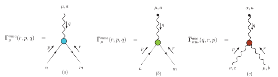
Figure 1: Diagrammatic representations of the fully dressed three-point vertices. We show in the panels $(a)$ the conventional ghost-gluon vertex ($\rm Q\overline{c}c$), $(b)$ the background ghost-gluon vertex (${\rm B\bar{c}c}\,$), and $(c)$ the background three-gluon vertex (${\rm BQQ}\,$), with their respective momenta conventions. All momenta are incoming, $q+r+p=0$.

Turning to the three-point sector of the theory, in Fig. 1 we show the full vertices relevant for our analysis: the conventional ghost-gluon vertex ($\rm Q\overline{c}c$) in panel $(a)$, the background ghost-gluon vertex ($\rm B\overline{c}c$) in panel $(b)$, and the background three-gluon vertex ($\rm BQQ$) in panel $(c)$.

Factoring out the corresponding color structures and the coupling $g$, we define the vertices ${\bm{\Gamma}}$ that will be used for the rest of this work as follows:

$$\Gamma_{\bar{c}^{m}c^{n}Q_{\mu}^{a}}(r,p,q) = -gf^{mna}{\bm{\Gamma}}_{\mu}(r,p,q)\,,$$

$$\Gamma_{\bar{c}^{m}c^{n}B_{\mu}^{a}}(r,p,q) = -gf^{mna}\widetilde{\bm{\Gamma}}_{\mu}(r,p,q)\,,$$

$$\Gamma_{\!B_{\alpha}^{a}Q_{\mu}^{b}Q_{\nu}^{c}}(q,r,p) = gf^{abc}\widetilde{\bm{\Gamma}}_{\alpha\mu\nu}(q,r,p)\,.$$ (3)

We now briefly summarize some basic properties of the aforementioned vertices. We start with the conventional ghost-gluon vertex, ${\bm{\Gamma}}_{\mu}(r,p,q)$, whose tensorial decomposition is given by

$${\bm{\Gamma}}_{\mu}(r,p,q)=B_{1}(r,p,q)r_{\mu}+B_{2}(r,p,q)q_{\mu}\,,$$ (4)

where $B_{1}(r,p,q)$ and $B_{2}(r,p,q)$ are the corresponding form factors. At tree-level, ${\bm{\Gamma}}_{\mu}^{(0)}=r_{\mu}$, and therefore $B_{1}^{(0)}=1$, and $B_{2}^{(0)}=0$. ${\bm{\Gamma}}_{\mu}(r,p,q)$ satisfies the STI

$${\bm{\Gamma}}_{\mu}(r,p,q)=r^{\nu}H_{\nu\mu}(r,p,q)\,,$$ (5)

where $H_{\nu\mu}(r,p,q)$ is the ghost-gluon scattering kernel Ball and Chiu (1980); Aguilar et al. (2019b).

Due to Taylor’s theorem Taylor (1971), in the limit of $p\to 0$, known as “Taylor kinematics” or “soft ghost limit” Fischer (2006); Aguilar et al. (2009, 2021b), the ghost-gluon vertex reduces to its tree-level value, i.e., ${\bm{\Gamma}}_{\mu}(r,0,-r)=r_{\mu}$. Similarly, under the assumption that $H_{\nu\mu}(r,p,q)$ contains no poles of the type $1/r^{2}$, from Eq. (5) follows that ${\bm{\Gamma}}_{\mu}(r,p,q)$ vanishes in the soft antighost limit, i.e., as $r\to 0$; then, from Eq. (4) we conclude that $B_{2}(0,-q,q)=0$.

Turning to $\widetilde{\bm{\Gamma}}_{\mu}(r,p,q)$, in complete analogy with Eq. (4) we have

$$\widetilde{\bm{\Gamma}}_{\mu}(r,p,q)=\widetilde{B}_{1}(r,p,q)r_{\mu}+\widetilde{B}_{2}(r,p,q)q_{\mu}\,;$$ (6)

its tree-level expression $\widetilde{\bm{\Gamma}}_{\mu}^{(0)}$ is given in Eq. (52), such that $\widetilde{B}_{1}^{(0)}=2$, and $\widetilde{B}_{2}^{(0)}=1$. Note that one of the distinctive features of $\widetilde{\bm{\Gamma}}_{\mu}(r,p,q)$ is the linear (Abelian) STI that it satisfies

$$q^{\mu}\,\widetilde{\bm{\Gamma}}_{\mu}(r,p,q)=D^{-1}(p)-D^{-1}(r)\,.$$ (7)

Finally, consider the ${\rm BQQ}\,$vertex, denoted by $\widetilde{\bm{\Gamma}}_{\alpha\mu\nu}(q,r,p)$. This vertex is a central component in SDE studies of the gluon propagator within the PT-BFM approach, and several of its main properties have been explored in the related literature, see, e.g.,  Binosi and Papavassiliou (2011). However, for the present study of the all-soft limit the only relevant characteristic of $\widetilde{\bm{\Gamma}}_{\alpha\mu\nu}(q,r,p)$ is its $\xi$-dependence at tree-level [see the Feynman rule for $\widetilde{\bm{\Gamma}}^{(0)}_{\alpha\mu\nu}$ given in Eq. (51)]. Specifically, we can decompose the full $\widetilde{\bm{\Gamma}}_{\alpha\mu\nu}(q,r,p)$ as

$$\widetilde{\bm{\Gamma}}_{\alpha\mu\nu}(q,r,p)=\widetilde{\Gamma}_{\alpha\mu\nu}(q,r,p)+\frac{1}{\xi}\left[g_{\alpha\nu}\,r_{\mu}-g_{\alpha\mu}\,p_{\nu}\right]\,,$$ (8)

where the second term on the r.h.s. is the $\xi$-dependent tree-level term. Then, combining Eq. (8) and Eq. (51), we see immediately that, at tree-level, $\widetilde{\Gamma}_{\alpha\mu\nu}^{(0)}(q,r,p)={\bm{\Gamma}}^{(0)}_{\alpha\mu\nu}(q,r,p)$, where ${\bm{\Gamma}}_{\alpha\mu\nu}^{(0)}(q,r,p)=g_{\mu\nu}(r-p)_{\alpha}+g_{\alpha\nu}(p-q)_{\mu}+g_{\alpha\mu}(q-r)_{\nu}$ is the standard tree-level expression of the conventional three-gluon vertex (QQQ).

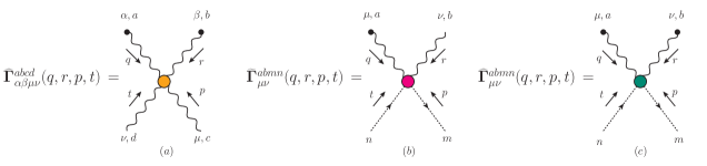
Figure 2: Diagrammatic representations of the fully dressed four-point functions: (a) ${\rm BBQQ}\,$, (b) ${\rm BQ\bar{c}c}\,$, and (c) ${\rm BB\bar{c}c}\,$. Notice that all momenta are incoming, i.e., $q+r+p+t=0$, and we have factored out $-ig^{2}$ following the definitions of Eq. (9).

We now turn our attention to the four-point sector of the theory. In Fig. 2 we show the three four-point vertices relevant for our analysis, namely the BBQQ vertex [panel (a)], the ${\rm BQ\bar{c}c}\,$vertex [panel (b)], and the ${\rm BB\bar{c}c}\,$vertex [panel (c)]. These vertices will be denoted as

$$\Gamma_{\!B_{\alpha}^{a}B_{\beta}^{b}Q_{\mu}^{c}Q_{\nu}^{d}}(q,r,p,t) = -ig^{2}\widehat{\bm{\Gamma}}^{abcd}_{\alpha\beta\mu\nu}(q,r,p,t)\,,$$

$$\Gamma_{\!B_{\mu}^{a}Q_{\nu}^{b}\bar{c}^{m}c^{n}}(q,r,p,t) = -ig^{2}{\widetilde{\bm{\Gamma}}}^{abmn}_{\mu\nu}(q,r,p,t)\,,$$

$$\Gamma_{\!B_{\mu}^{a}B_{\nu}^{b}\bar{c}^{m}c^{n}}(q,r,p,t) = -ig^{2}\widehat{\bm{\Gamma}}^{abmn}_{\mu\nu}(q,r,p,t)\,,$$ (9)

and their corresponding tree-level expressions may be found in Eqs. (1), (54), and (55), respectively.

Note that $\widehat{\bm{\Gamma}}^{abcd}_{\alpha\beta\mu\nu}(q,r,p,t)$ depends on $\xi$ already at tree level, and can be written as

$$\widehat{\bm{\Gamma}}^{abcd}_{\alpha\beta\mu\nu}(q,r,p,t)=\widehat{\Gamma}^{abcd}_{\alpha\beta\mu\nu}(q,r,p,t)+\frac{1}{\xi}\left[f^{acx}f^{xbd}g_{\alpha\mu}\,g_{\beta\nu}-f^{adx}f^{xbc}g_{\alpha\nu}\,g_{\beta\mu}\right]\,.$$ (10)

In addition, the vertex ${\widetilde{\bm{\Gamma}}}^{abmn}_{\mu\nu}(q,r,p,t)$ is related to the ${\bm{\Gamma}}_{\nu}(r,p,q)$ through the simple STI Aguilar and Papavassiliou (2006); Binosi and Papavassiliou (2008)

$$q^{\mu}{\widetilde{\bm{\Gamma}}}^{abmn}_{\mu\nu}(q,r,p,t)\!=\!f^{nax}f^{bmx}{\bm{\Gamma}}_{\nu}(p,q\!+\!t,r)+f^{nbx}f^{max}{\bm{\Gamma}}_{\nu}(q\!+\!p,t,r)+f^{nmx}f^{abx}{\bm{\Gamma}}_{\nu}(p,t,q\!+\!r)\,.$$ (11)

The vertex $\widehat{\bm{\Gamma}}^{abmn}_{\mu\nu}(q,r,p,t)$, which is central to our analysis, may be expanded as Pascual and Tarrach (1980); Binosi et al. (2014); Huber (2017)

$$\widehat{\bm{\Gamma}}^{abmn}_{\mu\nu}(q,r,p,t)=\sum_{i=1}^{10}\sum_{j=1}^{8}{T}_{ij}(q,r,p,t){\ell}^{i}_{\mu\nu}c^{abmn}_{j}\,,$$ (12)

where

$$\ell^{1}_{\mu\nu}=g_{\mu\nu}\,,$$

(13)

and

$$c_{1}^{abmn}=f^{anx}f^{mbx}\,,$$

(14)

At tree level, only $T^{(0)}_{11}=T^{(0)}_{12}=1$ are nonvanishing.

The Bose symmetry of $\widehat{\bm{\Gamma}}^{abmn}_{\mu\nu}(q,r,p,t)$ under the exchange of two background gluons, i.e., $(a,\mu,q)\leftrightarrow(b,\nu,r)$, imposes additional constraints on the form factors ${T}_{ij}(q,r,p,t)$. Specifically, 45 out of the 80 form factors $T_{ij}(q,r,p,t)$ can be written as permutations of the arguments of the remaining 35, e.g., $T_{73}(q,r,p,t)=T_{33}(r,q,p,t)$.

Of course, in the all-soft limit that we study, the tensorial structures collapse to $g_{\mu\nu}$, which, by virtue of the Bose symmetry, may be multiplied by $(f^{anx}f^{mbx}+f^{max}f^{bnx})$, $(\delta^{am}\delta^{nb}+\delta^{an}\delta^{bm})$, and $\delta^{ab}\delta^{mn}$. However, only the first color combination respects the ghost-antighost symmetry of the vertex, so that we finally arrive at the unique structure relevant for the all-soft limit, namely $(f^{anx}f^{mbx}+f^{max}f^{bnx})g_{\mu\nu}$.

Let us finally introduce the renormalization constants $Z_{i}$ that connect bare and renormalized quantities. In particular, we have Aguilar et al. (2013b, 2016)

$$\Delta_{{\scriptscriptstyle R}}(q^{2})=Z^{-1}_{A}\Delta(q^{2}),\qquad F_{{\scriptscriptstyle R}}(q^{2})=Z^{-1}_{c}F(q^{2}),\qquad g_{{\scriptscriptstyle R}}=Z_{g}^{-1}g\,,$$ (15)

and

$${\bm{\Gamma}}_{\mu}(r,p,q) :=Z_{1}^{-1}{\bm{\Gamma}}^{\rm{\scriptscriptstyle R}}_{\mu}(r,p,q)\,,\qquad\qquad\widetilde{\bm{\Gamma}}_{\mu\nu}(q,r,p,t):=\widetilde{Z}^{-1}_{4}\widetilde{\bm{\Gamma}}^{\rm{\scriptscriptstyle R}}_{\mu\nu}(q,r,p,t)\,,$$

$$\widetilde{\bm{\Gamma}}_{\mu}(r,p,q) :=\widetilde{Z}^{-1}_{1}\widetilde{\bm{\Gamma}}^{\rm{\scriptscriptstyle R}}_{\mu}(r,p,q)\,,\qquad\qquad\widehat{\bm{\Gamma}}_{\mu\nu}(q,r,p,t):=\widehat{Z}^{-1}_{4}\widehat{\bm{\Gamma}}^{\rm{\scriptscriptstyle R}}_{\mu\nu}(q,r,p,t)\,,$$ (16)

where we have omitted the color structures for simplicity.

By virtue of the various STIs relating the above Green’s functions, the renormalization constants satisfy the conditions

$$\widehat{Z}_{4}=\widetilde{Z}_{1}\,,\qquad\widetilde{Z}_{1}=Z_{c}\,,\qquad\widetilde{Z}_{4}=Z_{1}\,,\,\qquad Z^{-1}_{g}=Z_{1}^{-1}Z_{A}^{1/2}Z_{c}\,.$$ (17)

Note that, in the Landau gauge, the renormalization constant $Z_{1}$ is finite (cutoff-independent), as a consequence of Taylor’s theorem Taylor (1971).

III All-soft limit: an exact result

In this section we derive the exact all-soft limit of the vertex ${\widehat{\bm{\Gamma}}}^{abmn}_{\mu\nu}(q,r,p,t)$, by resorting to the simple STI that relates ${\widehat{\bm{\Gamma}}}^{abmn}_{\mu\nu}(q,r,p,t)$ with the $\widetilde{\bm{\Gamma}}_{\nu}$ of Eq. (6), namely

$$q^{\mu}\widehat{\bm{\Gamma}}_{\mu\nu}^{abmn}(q,r,p,t)\!=\!f^{abx}f^{mnx}\widetilde{\bm{\Gamma}}_{\nu}(p,t,q+r)+f^{anx}f^{bmx}\widetilde{\bm{\Gamma}}_{\nu}(p,q+t,r)+f^{amx}f^{nbx}\widetilde{\bm{\Gamma}}_{\nu}(q+p,t,r)\,.$$ (18)

Eq. (18) may be derived within the systematic approach provided by the Batalin-Vilkovisky formalism Batalin and Vilkovisky (1977, 1983); Binosi and Papavassiliou (2002, 2009). A more direct derivation relies on the observation that, at tree-level [see Eqs. (52) and (55)], if we contract $\widehat{\bm{\Gamma}}^{(0)abmn}_{\mu\nu}$ by $q^{\mu}$ and, with the aid of the Jacobi identity, add to the answer $(p-t)_{\nu}[f^{abx}f^{mnx}+f^{anx}f^{bmx}+f^{amx}f^{nbx}]=0$, we have

$$q^{\mu}\widehat{\bm{\Gamma}}^{(0)abmn}_{\mu\nu}=f^{abx}f^{mnx}\underbrace{(p-t)_{\nu}}_{\widetilde{\bm{\Gamma}}^{(0)}_{\nu}(p,t,q+r)}+f^{anx}f^{bmx}\underbrace{(p-t-q)_{\nu}}_{\widetilde{\bm{\Gamma}}^{(0)}_{\nu}(p,q+t,r)}+f^{amx}f^{nbx}\underbrace{(p-t+q)_{\nu}}_{\widetilde{\bm{\Gamma}}^{(0)}_{\nu}(q+p,t,r)}\,.$$ (19)

Since the STIs triggered with respect to a background leg maintain their tree-level form, the naive generalization of Eq. (19) leads us to Eq. (18).

The way to proceed with Eq. (18) is analogous to the typical derivation of a WI out of a STI: as the momentum that triggers the STI tends to zero, a Taylor expansion of both sides is carried out, followed by an appropriate matching of terms linear in $q$. In the case of the four-particle vertex $\widehat{\bm{\Gamma}}_{\mu\nu}^{abmn}(q,r,p,t)$ that we consider, it is convenient to choose as a point of departure the special kinematic configuration $(q,r,p,t)\to(q,-q,0,0)$. In that case, Eq. (18) reduces to

$$q^{\mu}\widehat{\bm{\Gamma}}_{\mu\nu}^{abmn}(q,-q,0,0)\!=\!f^{abx}f^{mnx}\widetilde{\bm{\Gamma}}_{\nu}(0,0,0)+f^{anx}f^{bmx}\widetilde{\bm{\Gamma}}_{\nu}(0,q,-q)+f^{amx}f^{nbx}\widetilde{\bm{\Gamma}}_{\nu}(q,0,-q)\,.$$ (20)

To begin with, it is clear that that $\widetilde{\bm{\Gamma}}_{\nu}(0,0,0)=0$, since it has just one Lorentz index and all momenta were set to zero.

Then, the second and third terms on the r.h.s of Eq. (20) correspond to the “soft antighost” (i.e.,  $r\to 0$ ) and “soft ghost” (or equivalently “Taylor kinematics” where $p\to 0$) limits of the background ghost-gluon vertex, $\widetilde{\bm{\Gamma}}_{\mu}$, respectively.

The derivation of the special exact relation that $\widetilde{\bm{\Gamma}}_{\mu}$, in the “soft ghost” kinematics satisfies, was shown in Aguilar et al. (2018b) using three different approaches. In what follows, we will sketch some of the main steps of the derivation based on the STI that $\widetilde{\bm{\Gamma}}_{\mu}$ satisfies, since we are using a different tensorial basis for $\widetilde{\bm{\Gamma}}_{\mu}$. These steps will be also relevant for the derivation of the “soft antighost” limit.

The starting point is the combination of the most general tensorial decomposition of $\widetilde{\bm{\Gamma}}_{\mu}$, written in Eq. (6), and the STI of Eq. (7) that $\widetilde{\bm{\Gamma}}_{\mu}$ satisfies, which lead us to

$$(q\cdot r)\widetilde{B}_{1}(r,p,q)+q^{2}\widetilde{B}_{2}(r,p,q)=D^{-1}(p)-D^{-1}(r)\,.$$ (21)

Next, assuming that there are no poles associated to the $r=0$ and $p=0$ limits; then, in the soft ghost limit ($p=0$ and $r=-q$) Eq. (21) becomes

$$\widetilde{B}_{1}(q,0,-q)-\widetilde{B}_{2}(q,0,-q)=F^{-1}(q)\,.$$ (22)

Thus, setting $p=0$ and $r=-q$ in Eq. (6) and in the sequence, using the Eq. (22), we find that in the soft ghost limit

$$\widetilde{\bm{\Gamma}}_{\mu}(q,0,-q)=q_{\mu}\left[\widetilde{B}_{1}(q,0,-q)-\widetilde{B}_{2}(q,0,-q)\right]=q_{\mu}F^{-1}(q)\,.$$ (23)

Similarly, in the soft antighost limit ($r=0$ and $p=-q$), Eq. (21) simplifies to

$$\widetilde{B}_{2}(0,q,-q)=F^{-1}(q)\,,$$ (24)

where we used Lorentz invariance to change the sign of the arguments of the scalar function $\widetilde{B}_{2}$. Then, substituting the above result in Eq. (6), we obtain the exact relation

$$\widetilde{\bm{\Gamma}}_{\mu}(0,q,-q)=-q_{\mu}\widetilde{B}_{2}(0,q,-q)=-q_{\mu}F^{-1}(q)\,.$$ (25)

Therefore, we find that both limits are related to each other as

$$\widetilde{\bm{\Gamma}}_{\mu}(q,0,-q)=-\widetilde{\bm{\Gamma}}_{\mu}(0,q,-q)=q_{\mu}F^{-1}(q)\,.$$ (26)

Let us mention in passing that the results of Eq. (26), derived above in full generality, may also be obtained from the standard gauge technique Ansatz Ball and Chiu (1980),

$$\widetilde{\bm{\Gamma}}_{\mu}(r,p,q)=\left[\frac{D^{-1}(p)-D^{-1}(r)}{p^{2}-r^{2}}\right](2r+q)_{\mu}+{\mathcal{A}}_{\rm T}(r,p,q)[(r\cdot q)q_{\mu}-q^{2}r_{\mu}]\,,$$ (27)

provided that the undetermined transverse (automatically conserved) part is well-behaved in the limit $q\to 0$.

Substituting the results of Eq. (26) into the r.h.s. of Eq. (20), we arrive at

$$q^{\mu}\widehat{\bm{\Gamma}}^{abmn}_{\mu\nu}(q,0,-q,0) =q_{\nu}(f^{max}f^{xbn}+f^{mbx}f^{xan})F^{-1}(q)\,,$$ (28)

which, upon expansion around $q=0$, yields the final exact result

$$\widehat{\bm{\Gamma}}^{abmn}_{\mu\nu}(0,0,0,0)=g_{\mu\nu}(f^{max}f^{bnx}+f^{mbx}f^{anx})F^{-1}(0)\,.$$ (29)

Clearly, at tree-level, when $F^{-1}(0)=1$, the above result reduces simply to the momentum-independent expression for $\widehat{\bm{\Gamma}}^{(0)abmn}_{\mu\nu}$ given in Eq. (55).

Finally, in terms of the form factors ${T}_{ij}(q,r,p,t)$ appearing in Eq. (12), the exact result of Eq. (29) implies that

$$T(0):=T_{11}(0,0,0,0)=T_{12}(0,0,0,0)=F^{-1}(0)\,.$$ (30)

The remaining form factors ${T}_{ij}(0,0,0,0)$ are undetermined, because their associated tensor structures vanish directly in the all-soft limit.

IV All-soft limit of the SDE

In this section we derive the all-soft limit of the vertex $\widehat{\bm{\Gamma}}^{abmn}_{\mu\nu}(q,r,p,t)$ from the SDE that it satisfies. This is a subtle exercise, mainly for two reasons: first, a series of key gauge cancellations must be implemented before the Landau gauge limit may be taken safely; and second, several instrumental properties of the vertices nested inside the Feynman diagrams of the SDE must be employed, in order for the result of Eq. (29) to emerge.

We find it convenient to set up the SDE with respect to the ghost field carrying the momentum $t$. According to the standard procedure, the ghost field is attached to all possible tree-level vertices containing it, while the remaining three fields connect to the diagram by means of appropriate dressed kernels. In the particular case that we consider there are two relevant tree-level vertices: the standard ${\rm Q\bar{c}c}\,$vertex, and the ${\rm BQ\bar{c}c}\,$vertex that is particular to the BFM. The resulting SDE is represented diagrammatically in Fig. 3, in terms of the five- and four-particle kernels, denoted by ${\cal K}^{abcme}_{5\,\mu\nu\rho}$ and ${\cal K}^{bcme}_{4\,\nu\rho}$, respectively; the crossed diagram obtained by interchanging the background gluons of $(b)$ is not shown.

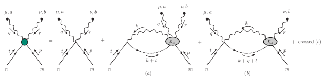
Figure 3: Diagrammatic representation of the SDE for the ${\rm BB\bar{c}c}\,$. The gray ellipses represent the five- and four-points kernels, ${\cal K}^{abcem}_{5\,\mu\nu\rho}$ and ${\cal K}^{bcem}_{4\,\mu\nu}$, respectively. The diagram obtained from $(b)$ through crossing of the gluon legs, $\mu,a\leftrightarrow\nu,b$, is not shown.

Each of the kernels ${\cal K}^{abcme}_{5\,\mu\nu\rho}$ and ${\cal K}^{bcme}_{4\,\nu\rho}$ consists of a component that sums up the one-particle reducible (1PR) terms, to be denoted by ${\cal T}^{abcme}_{5\;\mu\nu\rho}$ and ${\cal T}^{bcme}_{4\;\nu\rho}$, and a component containing all possible one-particle irreducible (1PI) contributions, to be denoted by ${\cal G}^{abcme}_{5\;\mu\nu\rho}$ and ${\cal G}^{bcme}_{4\;\nu\rho}$, respectively, as shown in Fig. 4. Thus, we have

$${\cal K}^{abcme}_{5\;\mu\nu\rho}={\cal T}^{abcme}_{5\;\mu\nu\rho}+\,{\cal G}^{abcme}_{5\;\mu\nu\rho}\,,\qquad\qquad{\cal K}^{bcme}_{4\;\nu\rho}={\cal T}^{bcme}_{4\;\nu\rho}+\,{\cal G}^{bcme}_{4\;\nu\rho}\,.$$ (31)

Note that ${\cal G}^{abcme}_{5\;\mu\nu\rho}$ coincides with the dressed loop-wise (skeleton) expansion of the 1PI five-point Green’s function $\langle 0|\,T\!\left[{B}^{a}_{\mu}\,{B}^{b}_{\nu}\,{Q}^{c}_{\rho}\,{\bar{c}}^{m}\,c^{e}\right]\!|0\rangle$, while ${\cal G}^{bcme}_{4\;\nu\rho}$ corresponds to the 1PI four-point function $\langle 0|\,T\!\left[{B}^{b}_{\nu}\,{Q}^{c}_{\rho}\,{\bar{c}}^{m}\,c^{e}\right]\!|0\rangle$.

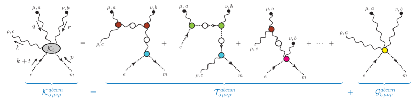
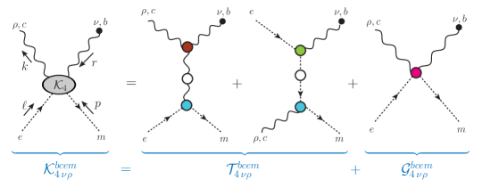
Figure 4: First row: The skeleton expansion of the five-particle kernel ${\cal K}^{abcem}_{5\,\mu\nu\rho}$ is shown as the sum of the 1PR and 1PI contributions, denoted by ${\cal T}^{abcem}_{5\;\mu\nu\rho}$ and ${\cal G}^{abcem}_{5\,\mu\nu\rho}$, respectively; the dots indicate additional 1PR graphs not shown. Second row: The corresponding contributions of ${\cal K}^{bcem}_{4\,\nu\rho}$, denoted by ${\cal T}^{bcem}_{4\;\nu\rho}$ and ${\cal G}^{bcem}_{4\,\nu\rho}$, respectively.

The renormalization of the SDE for the vertex $\widehat{\bm{\Gamma}}^{abmn}_{\mu\nu}(q,r,p,t)$ proceeds by introducing the renormalization relations given in Eqs. (15) and (II) into each of the graphs in Fig. 5, employing the constraints listed in Eq. (17). Then, the renormalized version of the vertex SDE reads

$$\widehat{\bm{\Gamma}}^{abmn}_{\mu\nu}(q,r,p,t)=Z_{c}\,\widehat{\bm{\Gamma}}^{(0)abmn}_{\mu\nu}-ig^{2}Z_{1}\sum{\rm all\,\,graphs}\,,$$ (32)

where all subscripts “R” have been suppressed in order to avoid notation clutter.

We next evaluate the all-soft limit of the diagrams given in Fig. 5. In doing so, the cancellation of terms proportional to $1/\xi$ must be carried out before the Landau limit, $\xi\to 0$, is taken.

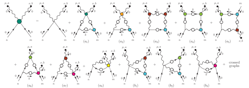
Figure 5: The diagrammatic representation of the SDE for the vertex ${\rm BB\bar{c}c}\,$, expanded in terms of 1PI vertices; crossed diagrams are not shown. Note that diagrams $(a_{i})$ with $i=1,2,\cdots,8$ originate from the expansion of the 1PR kernel in $(a)$ in Fig. 3, while $(b_{i})$ with $i=1,2,3$ come from $(b)$.

(i) We start by noticing that the diagrams $(a_{1})$, $(a_{4})$, $(a_{6})$, and $(b_{2})$ do not contain vertices with $\xi$-dependent tree-level expressions; therefore, the Landau gauge may be reached directly by setting $\xi=0$ throughout. Then, it is elementary to establish that $(a_{1})$, $(a_{4})$, and $(a_{6})$ vanish in the all-soft limit, $(p,q,r,t)=(0,0,0,0)$, because the sequence

$$(p+k)^{\sigma}\Delta_{\sigma\rho}(k)\xrightarrow[\text{}]{\text{$\xi=0$}}(p+k)^{\sigma}P_{\sigma\rho}(k)\Delta(k)\xrightarrow[\text{}]{\text{$p=0$}}k^{\sigma}P_{\sigma\rho}(k)\Delta(k)=0\,,$$ (33)

is triggered. As for graph $(b_{2})$, it vanishes because it contains the ghost-gluon vertex in the soft antighost limit, i.e., ${\bm{\Gamma}}_{\rho}(0,k,-k)=0$. Thus, in total,

$$(a_{1})^{abmn}_{\mu\nu}=(a_{4})^{abmn}_{\mu\nu}=(a_{6})^{abmn}_{\mu\nu}=(b_{2})^{abmn}_{\mu\nu}=0\,.$$ (34)

(ii) Diagrams $(a_{2})$, $(a_{3})$, $(a_{5})$, and $(b_{1})$ eventually vanish, because they all contain the ghost-gluon vertex in the soft antighost limit. However, since these graphs contain tree-level vertices with terms proportional to $1/\xi$, a limiting procedure must be followed in order to safely implement the Landau gauge, thus triggering the result ${\bm{\Gamma}}_{\rho}(0,k,-k)=0$. To that end, in the case of graphs $(a_{2})$, $(a_{3})$, and $(a_{5})$ note that we “gain” a power of $\xi$ by employing $(p+k)^{\sigma}\Delta_{\sigma\rho}(k)\xrightarrow[\text{}]{\text{$p=0$}}k^{\sigma}\Delta_{\sigma\rho}(k)=\xi\,k_{\rho}/k^{2}$. The presence of this $\xi$ makes all $\xi$-independent terms vanish, as $\xi\to 0$. Furthermore, it cancels the $1/\xi$ terms originating from the vertices, furnishing finite expressions, given by

$$(a_{2})^{abmn}_{\mu\nu} \!= \!g^{4}c_{1}^{cndm}\!\!\int_{k}\!\!\left(\frac{k^{\rho}}{k^{2}}\right)D(k)\Delta^{\sigma\lambda}(k){\bm{\Gamma}}_{\lambda}(0,-k,k)\left[c_{1}^{adbc}g_{\mu\sigma}g_{\nu\rho}-c_{1}^{acbd}g_{\mu\rho}g_{\nu\sigma}\right]\,,$$

$$(a_{3})_{\mu\nu}^{abmn} = g^{4}c_{1}^{cdba}c_{1}^{dcnm}\int_{k}\left(\frac{k^{\gamma}}{k^{2}}\right)D(k){\bm{\Gamma}}_{\rho}(0,k,-k)[g_{\mu\gamma}k_{\beta}+g_{\mu\beta}k_{\gamma}]\times$$ (35)

$$\qquad\qquad\qquad\left[\Delta^{\rho\sigma}(k)\Delta^{\alpha\beta}(k)\widetilde{\Gamma}_{\nu\sigma\alpha}(0,k,-k)\,+\left(\frac{k^{\beta}}{k^{2}}\right)\Delta^{\rho}_{\nu}(k)+\left(\frac{k^{\rho}}{k^{2}}\right)\Delta^{\beta}_{\nu}(k)\right]\,,$$

$$(a_{5})_{\mu\nu}^{abmn} = g^{4}c_{1}^{cdma}c_{1}^{ndbc}\int_{k}\left(\frac{k_{\rho}}{k^{2}}\right)\Delta_{\alpha\beta}(k)D^{2}(k)\widetilde{\bm{\Gamma}}_{\nu}(-k,k,0){\bm{\Gamma}}_{\beta}(0,k,-k)(g_{\mu\rho}k_{\alpha}+g_{\mu\alpha}k_{\rho})\,.$$

The vertex $\widetilde{\Gamma}_{\nu\sigma\alpha}(0,k,-k)$, appearing in the second equation, has been defined in Eq. (8), whereas the factor $c_{1}^{cndm}$ is given in Eq. (14). In addition, we have introduced the integral measure

$$\int_{k}:=\frac{1}{(2\pi)^{4}}\int\!\!\differential[4]{k}\,,$$ (36)

where the use of a symmetry-preserving regularization scheme is implicitly understood.

Since at this point we may set $\xi=0$ in the expressions of Eq. (35), the result ${\bm{\Gamma}}_{\rho}(0,k,-k)=0$ makes them all vanish.

Turning to $(b_{1})$, the term ${\bm{\Gamma}}_{\nu\rho\sigma}^{(0)}(0,k,-k)$ of the BFM tree-level vertex $\widetilde{\bm{\Gamma}}_{\nu\rho\sigma}^{(0)}(0,k,-k)$ simply yields the standard Landau gauge result, denoted by $(b_{11})$, while the term $\xi^{-1}(g_{\nu\sigma}k_{\rho}+g_{\nu\rho}k_{\sigma})$, once contracted with the adjacent gluon propagators, yields a finite contribution, denoted by $(b_{12})$, given by

$$(b_{12})_{\mu\nu}^{abmn}=g^{4}c_{1}^{gcmb}c_{1}^{cnga}g_{\mu\beta}\int_{k}D(k){\bm{\Gamma}}_{\rho}(0,k,-k)\left[\left(\frac{k^{\beta}}{k^{2}}\right)\Delta^{\rho}_{\nu}(k)+\left(\frac{k^{\rho}}{k^{2}}\right)\Delta^{\beta}_{\nu}(k)\right]\,.$$ (37)

Since both $(b_{11})$ and $(b_{12})$ contain the vertex ${\bm{\Gamma}}_{\rho}(0,k,-k)=0$, they both vanish when $\xi=0$. Thus, we finally have

$$(a_{2})^{abmn}_{\mu\nu}=(a_{3})^{abmn}_{\mu\nu}=(a_{5})^{abmn}_{\mu\nu}=(b_{1})^{abmn}_{\mu\nu}=0\,.$$ (38)

(iii) The treatment of diagram $(a_{8})$, which contains all 1PI corrections of the five-particle kernel, denoted by ${\cal G}^{abcme}_{5\,\mu\nu\rho}$, requires particular care. In what follows we explain why, in the all-soft limit, $(a_{8})=0$.

Since ${\cal G}^{abcme}_{5\,\mu\nu\rho}$ is computed using the BFM Feynman rules of Table 1, it is clear that individual diagrams may contain contributions proportional to $1/\xi$. Nonetheless, certain powerful formal properties guarantee that, due to massive cancellations among different diagrams, the entire ${\cal G}^{abcme}_{5\,\mu\nu\rho}$ contains no such terms, and therefore, the Landau-gauge limit may be safely implemented.

The rather technical demonstration of the above statement proceeds by appealing to the special relations known as Background-Quantum identities (BQIs) Grassi et al. (2001); Binosi and Papavassiliou (2002, 2009), derived through appropriate functional differentiation of the STI functional within the Batalin-Vilkovisky quantization formalism Batalin and Vilkovisky (1977, 1983). In particular, the BQIs express Green’s functions containing background fields ($B$) in terms of (i) conventional Green’s functions containing quantum fields ($Q$) and (ii) auxiliary Green’s functions involving the so-called “antifields” and “background sources”, arising from interaction terms particular to the aforementioned formalism. The special Feynman rules describing these latter Green’s functions may be found in Figs. (B.3)-(B.4) of Binosi and Papavassiliou (2009); their most relevant feature for our purposes is that they are $\xi$-independent.

Note that the exact form of the BQI that ${\cal G}^{abcme}_{5\,\mu\nu\rho}$ satisfies is not required for the argument that we present; it suffices to know that the BQI relates ${\cal G}^{abcme}_{5\,\mu\nu\rho}$ to a finite set of Green’s functions, all of which are regular as $\xi\to 0$. Consequently, the limit $\xi\to 0$ of ${\cal G}^{abcme}_{5\,\mu\nu\rho}$ is completely well-defined. The immediate upshot of the above result is that the all-soft limit of diagram $(a_{8})$ vanishes, simply because the Landau gauge may be taken directly, thus triggering the sequence given in Eq. (33).

(iv) We finally arrive at the contributions that survive the all-soft limit: they originate from diagrams $(a_{7})$ and $(b_{3})$, together with their crossed counterparts, to be denoted by $(a_{7}^{c})$ and $(b_{3}^{c})$, respectively.

Both $(a_{7})$ and $(b_{3})$ contain ${\cal G}^{abcme}_{4\,\nu\rho}$, namely the 1PI Green’s function $\langle 0|\,T\!\left[{B}^{b}_{\nu}\,{Q}^{c}_{\rho}\,{\bar{c}}^{m}\,c^{e}\right]\!|0\rangle$. The arguments presented in (iii) for ${\cal G}^{abcme}_{5\,\mu\nu\rho}$ apply unaltered in the case of ${\cal G}^{abcme}_{4\,\nu\rho}$, and the Landau gauge limit may be taken directly in it. Since the product $\widetilde{\bm{\Gamma}}_{\mu\rho^{\prime}\sigma^{\prime}}^{(0)}(0,k,-k)\Delta_{\rho^{\prime}\rho}(k)\Delta_{\sigma^{\prime}\sigma}(k)$ is finite as $\xi\to 0$, diagram $(a_{7})$ is nonvanishing, and the same is true for $(a_{7}^{c})$. Similarly, in $(b_{3})$ the ${\cal G}^{abcme}_{4\,\nu\rho}$ is connected to the rest of the diagram with propagators and vertices that are regular and nonvanishing as $\xi\to 0$, and the same happens with $(b_{3}^{c})$. The final individual contributions are given by

$$(a_{7})_{\mu\nu}^{abmn} =f^{ebx}f^{dnx}\int_{k}\Delta(k)D(k)\,P_{\nu}^{\alpha}(k)\,\widetilde{\bm{\Gamma}}^{adme}_{\mu\alpha}(0,-k,0,k)\,,$$

$$(b_{3})_{\mu\nu}^{abmn} =f^{eax}f^{dnx}\int_{k}\Delta(k)D(k)\,P_{\mu}^{\alpha}(k)\,\widetilde{\bm{\Gamma}}^{bdme}_{\nu\alpha}(0,-k,0,k)\,,$$

$$(a_{7}^{c})_{\mu\nu}^{abmn} =f^{enx}f^{bdx}\int_{k}\Delta(k)D(k)\,P_{\nu}^{\alpha}(k)\,\widetilde{\bm{\Gamma}}^{adme}_{\mu\alpha}(0,-k,0,k)\,,$$

$$(b_{3}^{c})_{\mu\nu}^{abmn} =f^{enx}f^{adx}\int_{k}\Delta(k)D(k)\,P_{\mu}^{\alpha}(k)\,\widetilde{\bm{\Gamma}}^{bdme}_{\nu\alpha}(0,-k,0,k)\,.$$ (39)

As a consequence of the considerations presented in (i)-(iv), the all-soft limit of Eq. (32) is given by

$$\widehat{\bm{\Gamma}}^{abmn}_{\mu\nu}(0,0,0,0)=Z_{c}\widehat{\bm{\Gamma}}^{(0)abmn}_{\mu\nu}-ig^{2}Z_{1}\left[(a_{7})+(a_{7}^{c})+(b_{3})+(b_{3}^{c})\right]_{\mu\nu}^{abmn}\,.$$ (40)

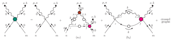
Figure 6: The diagrammatic representation of the SDE for the ${\rm BB\bar{c}c}\,$in the all-soft limit.

The next step consists in determining $\widetilde{\bm{\Gamma}}_{\mu\alpha}^{adme}(0,-k,0,k)$, the common ingredient in all integrals appearing in Eq. (IV). To that end, consider the STI in (11), and implement the special kinematic configuration $(q,r,p,t)\to(q,-k,-q,k)$, such that

$$q^{\mu}\widetilde{\bm{\Gamma}}^{adme}_{\mu\alpha}(q,-k,-q,k) = f^{eax}f^{dmx}{\bm{\Gamma}}_{\alpha}(-q,q+k,-k)+f^{edx}f^{max}{\bm{\Gamma}}_{\alpha}(0,k,-k)$$ (41)

$$+ f^{emx}f^{adx}{\bm{\Gamma}}_{\alpha}(-q,k,q-k)\,.$$

We then carry out a Taylor expansion of both sides around $q=0$. It is elementary to show that the zeroth order in $q$ vanishes on the r.h.s. because it is proportional to the Jacobi identity, while the coefficients of the linear terms are related by

$$\widetilde{\bm{\Gamma}}^{adme}_{\mu\alpha}(0,-k,0,k) = f^{aex}f^{dmx}\left\{\frac{\partial}{\partial q^{\mu}}\left[B_{1}(-q,q+k,-k)q_{\alpha}+B_{2}(-q,q+k,-k)k_{\alpha}\right]\right\}_{q=0}$$ (42)

$$+f^{mex}f^{adx}\left\{\frac{\partial}{\partial q^{\mu}}\left[B_{1}(-q,k,q-k)q_{\alpha}+B_{2}(-q,k,q-k)(q-k)_{\alpha}\right]\right\}_{q=0}\,,$$

where we have used that the momentum $k$ is independent of $q$. Then, since $B_{2}(0,k,-k)=0$ [see discussion after Eq. (5)], we arrive at

$$\widetilde{\bm{\Gamma}}^{adme}_{\mu\alpha}(0,-k,0,k)=g_{\mu\alpha}f^{amx}f^{dex}B_{1}(0,k,-k)+\cdots\,,$$ (43)

where the ellipsis denotes terms proportional to $k_{\alpha}$, which will be annihilated upon contraction with the projectors $P_{\nu}^{\alpha}(k)$ in Eq. (IV).

Substituting Eq. (43) into Eq. (IV), and employing the Jacobi identity together with the identity $f^{abe}f^{abx}=C_{\mathrm{A}}\delta^{ex}$, where $C_{\mathrm{A}}$ is the Casimir eigenvalue of the adjoint representation [$N$ for SU($N$)], and using that $P_{\mu}^{\mu}(k)=3$, one arrives at the final result

$$\widehat{\bm{\Gamma}}^{abmn}_{\mu\nu}(0,0,0,0)=g_{\mu\nu}(f^{max}f^{xbn}+f^{mbx}f^{xan})\left\{Z_{c}+i\frac{3}{4}g^{2}C_{\rm A}\,Z_{1}\!\int_{k}\!\Delta(k)D(k)B_{1}(0,k,-k)\right\}\,,$$ (44)

or, equivalently, in terms of the form factor $T(0)$ defined in Eq. (30)

$$T(0)=Z_{c}+i\frac{3}{4}g^{2}C_{\rm A}\,Z_{1}\!\int_{k}\!\Delta(k)D(k)B_{1}(0,k,-k)\,.$$ (45)

In order to make contact with the exact results of Eqs. (29) and (30) we need to employ the SDE that governs the ghost dressing function $F(q)$ in the Landau gauge, depicted in Fig. 7. Using for ${\bm{\Gamma}}_{\mu}(-q,k+q,-k)$ the decomposition given in Eq. (4), the ghost SDE is given by

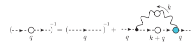
Figure 7: The SDE for the ghost propagator. The white circles represent the full gluon and ghost propagators, while the blue one denotes the full ghost-gluon vertex.

$$F^{-1}(q)=Z_{\rm c}+ig^{2}C_{\rm A}Z_{1}\int_{k}D(k+q)\Delta(k)f(k,q)B_{1}(-q,k+q,-k)\,,$$ (46)

where the renormalization constants $Z_{\rm c}$ and $Z_{1}$ have been defined in Eqs. (15) and (II), respectively, and $f(k,q):=1-(k\dotproduct q)^{2}/k^{2}q^{2}$.

It is then elementary to demonstrate by setting $q=0$ into Eq. (46) that

$$F^{-1}(0)=T(0)\,.$$ (47)

Thus, as announced, the result of (29) is recovered from the SDE of the vertex $\widehat{\bm{\Gamma}}^{abmn}_{\mu\nu}(q,r,p,t)$.

We emphasize that throughout the entire demonstration leading to Eq. (44), together with the subsequent equality in Eq. (47), no approximations have been employed. The results obtained are therefore exact, and represent a rather special occurrence within the SDE formalism.

V Estimating truncation errors

In this section we explore the implications of a simple truncation implemented at the level of Eq. (45), and estimate the associated errors by comparing the answers with the exact result of Eq. (30). The main points of this analysis may be summarized as follows.

(i) We approximate the ghost-gluon form factor $B_{1}(r,p,q)$ by its tree-level value, i.e., we set $B_{1}(r,p,q)=1$, and determine the error induced by this simplification to $T(0)$, in two different situations:

(a) the ghost propagator $D(k)$ entering into Eq. (45) is self-consistently obtained from its own SDE, namely Eq. (46) solved with $B_{1}(r,p,q)=1$,

and

(b) the ghost propagator $D(k)$ is treated as an external input, obtained from lattice simulations; it is substituted into Eq. (45), which is subsequently evaluated with $B_{1}(0,k,-k)=1$.

(ii) Note that, in order to simplify the analysis, in both cases the gluon propagator $\Delta(k)$ will be an external input, obtained from the combined set of lattice data of Bogolubsky et al. (2009); Boucaud et al. (2017, 2018); Aguilar et al. (2021b); the corresponding fit, shown on the left panel of Fig. 8, is given by Eqs. (B5) and (B6) in Aguilar et al. (2021b). We stress that the lattice data for both the gluon propagator and the ghost dressing function have been cured from discretization artifacts and finite-size effects Duarte et al. (2016); Boucaud et al. (2017, 2018); Duarte et al. (2017).

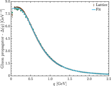
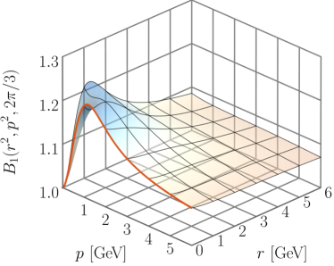
Figure 8: Left panel: The lattice data of Bogolubsky et al. (2009); Boucaud et al. (2017, 2018); Aguilar et al. (2021b) (circles), and the corresponding fit (blue continuous curve) for the gluon propagator, $\Delta(q)$. Right panel: The ghost-gluon form factor $B_{1}(r^{2},p^{2},2\pi/3)$ in general kinematics for a fixed value of angle $\varphi=2\pi/3$. The orange curve highlights the soft antighost limit of $B_{1}(0,p,-p)$, entering in Eq. (45).

(iii) As far as the truncation errors are concerned, the main difference between the two cases is that in (a) the error made when setting $B_{1}(r,p,q)=1$ affects the result for $T(0)$ nonlinearly, while in (b) the effect is practically linear. Specifically, in (a) the error induced to $T(0)$ by the corresponding error in $B_{1}$ is twofold: direct, through the slice $B_{1}(0,k,-k)$ in Eq. (45), and indirect, through the entire $B_{1}(-q,k+q,-k)$ that enters in the SDE that determines $D(k)$ [see Eq. (46)]. The difference between the two cases is that in (b) the indirect error is eliminated, since $D(k)$ is fixed from the lattice, and coincides with the answer obtained from the full treatment of the ghost SDE.

(iv) The result obtained from Eq. (45) for the cases (a) and (b), to be denoted by $T_{a}(0)$ and $T_{b}(0)$, respectively, will be compared with the exact result $F^{-1}(0)$; its benchmark value, to be denoted by $F^{-1}_{\!{\scriptscriptstyle L}}(0)$, is taken from the lattice simulation of Bogolubsky et al. (2009); Boucaud et al. (2018). The corresponding relative error, denoted by $\delta$, is defined as

$$\delta_{i}=\frac{\left|T_{i}(0)-F^{-1}_{\!{\scriptscriptstyle L}}(0)\right|}{F^{-1}_{\!{\scriptscriptstyle L}}(0)}\times 100\%\,,\,\,\,\qquad i=a,b\,.$$ (48)

(v) All relevant quantities are renormalized using the momentum subtraction (MOM) scheme, where the renormalized two-point functions acquire their tree-level values at the subtraction point $\mu$, i.e., $\Delta^{-1}(\mu)=\mu^{2}$ and $F(\mu)=1$. Within MOM we employ the special case of the so-called Taylor scheme Boucaud et al. (2009, 2011); von Smekal et al. (2009), which imposes the additional condition that the renormalized ghost-gluon vertex reduces to tree-level in the soft ghost kinematics, i.e., ${\bm{\Gamma}}_{\mu}(r,0,-r)=r_{\mu}$. This last condition fixes the (finite) ghost-gluon renormalization constant at the special value $Z_{1}=1$. In our computations, the subtraction point is chosen to be $\mu=4.3$ GeV; the corresponding value for $\alpha_{s}(\mu)=g^{2}/4\pi$ is $\alpha_{s}(4.3\,\rm GeV)=0.244$ Aguilar et al. (2021b).

(vi) It is instructive to compare the approximation $B_{1}(r,p,q)=1$ with the full $B_{1}(r,p,q)$ in general kinematics, obtained from a detailed SDE study of the ghost-gluon vertex Aguilar et al. (2021b). To that end, in the right panel of Fig. 8 we show a representative result for $B_{1}(r^{2},p^{2},\varphi)$, where $\varphi$ is the angle between $r$ and $p$, and we choose $\varphi=2\pi/3$. When $r\approx p\approx\mbox{$1.2$~{}GeV}$, $B_{1}$ displays a moderate peak of approximately $22\%$ over the tree-level value. On the other hand, when both momenta vanish, $B_{1}$ reduces to its tree-level value. On the same plot we highlight by the continuous orange line the soft antighost limit $B_{1}(0,p,-p)$, entering in Eq. (45).

(vii) For the implementation of the truncation mentioned in case (a), consider the ghost SDE in Eq. (46) , with $Z_{1}=1$ in the Taylor scheme. Clearly, for the numerical analysis, the Euclidean space versions of all expressions must be used; for the standard conversion rules, see e.g., Eq. (5.1) of Aguilar et al. (2019b).

Let us first emphasize that when the complete $B_{1}(-q,k+q,-k)$ is employed as input, together with the $\Delta(k)$ mentioned in (ii) and the $\alpha_{s}(\mu)$ in (v), Eq. (46) returns a solution for $F(q)$ that is in excellent agreement with the lattice data of Boucaud et al. (2018), see blue continuous curve in the left panel of Fig. 9 Aguilar et al. (2021b). From this curve we may directly deduce that the benchmark value is given by $F^{-1}_{\!{\scriptscriptstyle L}}(0)=0.344$ (for $\mu=4.3$ GeV).

Next, we implement the approximation $B_{1}(-q,k+q,-k)=1$ in Eq. (46), keeping $\Delta(k)$ and $\alpha_{s}(\mu)$ fixed. The resulting integral equation is given by

$$F^{-1}(q)=ig^{2}C_{\rm A}\int_{k}\Delta(k)\left[D(k+q)f(k,q)-D(k+\mu)f(k,\mu)\right]\,,$$ (49)

and the corresponding solution, to be denoted by $F_{a}(q)$, is shown as the red dashed curve in the left panel of Fig. 9. It is clear that $F_{a}(q)$ deviates considerably from the lattice results; in particular, at the origin we have the value $F^{-1}_{a}(0)=0.501$. Then, by virtue of Eq. (47), we have that $T_{a}(0)=F^{-1}_{a}(0)$, and employing Eq. (48) we find that the corresponding relative error is given by $\delta_{a}=47.5\%$.

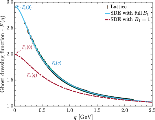
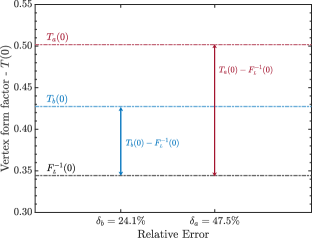
Figure 9: Left panel: Lattice data for the ghost dressing function from Boucaud et al. (2018) (circles), together with SDE results using the full $B_{1}$ (blue continuous curve) or its tree-level value (red dashed curve). Right panel: Comparison of the exact value for $T(0)$ with corresponding values obtained when we use in the Eq. (45) the two curves for $F(q)$ shown in the left panel.

(viii) We now turn to the truncation of case (b). In order to obtain the relative error we simply need to evaluate the integral of Eq. (45) with $B_{1}(0,k,-k)=1$, but setting $D(q)\to D_{\!{\scriptscriptstyle L}}(q)=F_{\!{\scriptscriptstyle L}}(q)/q^{2}$, namely the lattice (and full SDE) result for the ghost propagator. Thus, the integral to be determined is given by

$$T_{b}(0)=ig^{2}C_{\rm A}\int_{k}\Delta(k)\left[D_{\!{\scriptscriptstyle L}}(k+q)f(k,q)-D_{\!{\scriptscriptstyle L}}(k+\mu)f(k,\mu)\right]\,.$$ (50)

It is clear that this “hybrid” treatment invalidates the equality of Eq. (47), since the r.h.s. of Eq. (50) does not coincide with the $q=0$ limit of any ghost SDE; thus, $T_{b}(0)\neq F_{\!{\scriptscriptstyle L}}(0)$. In particular, using in Eq. (50) the same $\Delta(k)$ and $\alpha_{s}(\mu)$ as before, together with a fit to the lattice data for $F_{\!{\scriptscriptstyle L}}(q)$, one obtains $T_{b}(0)=0.427$, and the associated relative error computed from Eq. (48) is $\delta_{b}=24.1\%$.

(ix) The results derived in this section are pictorially summarized in the right panel of Fig. 9. It is clear that case (b) leads to a considerably smaller error, since the treatment of the ghost dressing function as an external input linearizes the dependence of $T(0)$ on $B_{1}$. In fact, the relative error $\delta_{b}=24.1\%$ is very close to the $22.1\%$ that separates the peak in $B_{1}$ from the tree-level value [see Fig. 8 and comments in (vi)]. This notable reduction in the error with respect to case (a) suggests that the hybrid treatment may be preferable, albeit theoretically less rigorous.

VI Discussion and Conclusions

In the present study we have considered the SDE of the special four-particle vertex that controls the interaction of two background gluons with a ghost-antighost pair (${\rm BB\bar{c}c}\,$vertex). We focused on the deep infrared limit, where all incoming momenta vanish. In this extreme limit, the form factor of the vertex may be determined exactly by virtue of the Abelian STI that it satisfies. In particular, the two surviving form factors are expressed in terms of two- and three-point functions, but without contributions from ghost-gluon kernels. This central result is recovered from the SDE by exploiting the Abelian STIs of the various vertices nested inside the diagrammatic expansion, and making repeated use of Taylor’s theorem. The aforementioned exact result, in turn, allows for the determination of the error associated with two related, but inherently distinct truncation procedures.

The realization of the WI at the level of the SDE, presented in Sec. III, is particularly noteworthy, combining concepts and techniques in a novel way, not previously presented in the literature. This construction highlights the importance of incorporating into the SDEs vertices that satisfy the constraints imposed by the fundamental symmetries of the theory, such as the STIs and Taylor’s theorem. In addition, it exposes the tight connections and delicate balance among the various SDE components, necessary for maintaining certain basic relations intact.

In this context, note that in Eq. (45), the dependence of $T(0)$ on the form factor $B_{1}$ of the ghost-gluon vertex ${\bm{\Gamma}}_{\mu}(r,p,q)$ does not originate from the graphs ($a_{1}$), ($a_{2}$), ($a_{3}$), ($a_{4}$), ($a_{5}$), ($b_{1}$), and ($b_{2}$) in Fig. 5, which contain the ${\bm{\Gamma}}_{\mu}(r,p,q)$ explicitly, since they all vanish in the all-soft limit, see Sec. IV. Instead, the answers stem from graphs ($a_{7}$) and ($b_{3}$), which have no explicit dependence on this form factor, but contain the vertex $\widetilde{\bm{\Gamma}}_{\mu\alpha}^{adme}(0,-k,0,k)$, whose WI in Eq. (43) induces the final dependence of $T(0)$ on $B_{1}$.

SDE calculations are often simplified by using lattice results as inputs for certain basic Green’s functions, and one of the truncations considered in this study [case (b) in item (i) of Sec. V] is motivated by this particular practice. In the present analysis, we found that this procedure clearly lowers the error induced to $T(0)$ by the uncertainty in $B_{1}$. To be sure, the actual amount of error reduction achieved may be atypically high (a factor of two), owing mostly to the enhanced sensitivity of the ghost SDE on $B_{1}$. An analogous study at the level of the gluon propagator is likely to produce a milder dependence on $B_{1}$, and thus, a more moderate improvement; on the other hand, the SDE of the gluon propagator depends on other poorly known Green’s functions, such as the four-gluon vertex Driesen and Stingl (1999); Kellermann and Fischer (2008); Binosi et al. (2014); Cyrol et al. (2015); Eichmann et al. (2015); Huber (2017, 2020b); Catumba (2021). Thus, even though no rigorous conclusions may be drawn, the use of lattice inputs in SDEs emerges as an advantageous option, because it reduces the number of active coupled equations and lowers the overall error. In addition, advances in techniques and procedures used for the elimination of discretization artifacts and finite-size effects from the data Duarte et al. (2016); Boucaud et al. (2017, 2018); Duarte et al. (2017) put the synergy between (gauge-fixed) lattice simulations and SDEs on firmer theoretical ground.

Undoubtedly, the BFM provides an excellent testing ground for the set of ideas presented in this work, mainly due to the ghost-free STIs satisfied by the relevant Green’s functions. It would be interesting to carry out lattice simulations directly in the BFM Dashen and Gross (1981); Luscher and Weisz (1995), following the formalism introduced in Cucchieri and Mendes (2012); Binosi and Quadri (2012).

VII Acknowledgments

The work of A. C. A. and B. M. O. are supported by the CNPq grants 307854/2019-1 and 141409/2021-5, respectively. A. C. A also acknowledges financial support from the FAPESP project 2017/05685-2 and 464898/2014-5 (INCT-FNA). J. P. is supported by the Spanish MICINN grant PID2020-113334GB-I00 and the regional Prometeo/2019/087 from the Generalitat Valenciana.

Appendix A Feynman rules for BFM vertices

	$$\widetilde{\bm{\Gamma}}_{\alpha\mu\nu}^{(0)}(q,r,p)=g_{\mu\nu}(r-p)_{\alpha}+g_{\alpha\nu}(p-q)_{\mu}+g_{\alpha\mu}(q-r)_{\nu}+\xi^{-1}(g_{\alpha\nu}r_{\mu}-g_{\alpha\mu}p_{\nu})\,,\vspace{-5cm}$$ (51)
	$$\widetilde{\bm{\Gamma}}^{(0)}_{\mu}(r,p,q)=(r-p)_{\mu}\,,\vspace{-4cm}$$ (52)
	$\displaystyle\widehat{\bm{\Gamma}}^{(0)abcd}_{\alpha\beta\mu\nu}=f^{adx}f^{xcb}\left(g_{\alpha\mu}g_{\beta\nu}-g_{\alpha\beta}g_{\mu\nu}\right)+f^{abx}f^{xdc}\left(g_{\alpha\nu}g_{\beta\mu}-g_{\alpha\mu}g_{\beta\nu}\right)$ $\displaystyle+$ $\displaystyle f^{acx}f^{xdb}\left(g_{\alpha\nu}g_{\beta\mu}-g_{\alpha\beta}g_{\mu\nu}\right)+\xi^{-1}(f^{adx}f^{xbc}g_{\alpha\nu}g_{\beta\mu}-f^{acx}f^{xdb}g_{\alpha\mu}g_{\beta\nu}),\vspace{-7cm}$
	$$\widetilde{\bm{\Gamma}}^{(0)abmn}_{\mu\nu}=f^{max}f^{xbn}g_{\mu\nu}\,,\vspace{-5.5cm}$$ (54)
	$$\widehat{\bm{\Gamma}}^{(0)abmn}_{\mu\nu}=g_{\mu\nu}\left(f^{max}f^{bnx}+f^{mbx}f^{anx}\right)\,.\vspace{-5.5cm}$$ (55)

Table 1: The diagrammatic representations of the new vertices appearing in the BFM and their respective Feynman rules at tree-level Binosi and Papavassiliou (2009). Notice that for the three-point functions we have factored out the coupling $g$ and their respective color structure, following the definitions of Eq. (3), while for the four-point functions, we have factored out only $-ig^{2}$ as shown in Eq. (9).

References

- Dyson (1949) F. J. Dyson, Phys. Rev. 75, 1736 (1949).
- Schwinger (1951a) J. S. Schwinger, Proc. Nat. Acad. Sci. 37, 452 (1951a).
- Schwinger (1951b) J. S. Schwinger, Proc. Nat. Acad. Sci. 37, 455 (1951b).
- Rivers (1988) R. J. Rivers, Path integral methods in quantum field theory, Cambridge Monographs on Mathematical Physics (Cambridge University Press, 1988).
- Itzykson and Zuber (1980) C. Itzykson and J. B. Zuber, Quantum Field Theory, International Series in Pure and Applied Physics (New York, USA: Mcgraw-Hill 705 p., 1980).
- Roberts and Williams (1994) C. D. Roberts and A. G. Williams, Prog. Part. Nucl. Phys. 33, 477 (1994).
- Alkofer and von Smekal (2001) R. Alkofer and L. von Smekal, Phys. Rept. 353, 281 (2001).
- Maris and Roberts (2003) P. Maris and C. D. Roberts, Int. J. Mod. Phys. E12, 297 (2003).
- Fischer (2006) C. S. Fischer, J. Phys. G 32, R253 (2006).
- Binosi and Papavassiliou (2009) D. Binosi and J. Papavassiliou, Phys. Rept. 479, 1 (2009).
- Binosi and Papavassiliou (2008) D. Binosi and J. Papavassiliou, J. High Energy Phys. 11, 063 (2008).
- Huber (2020a) M. Q. Huber, Phys. Rept. 879, 1 (2020a).
- Dorey and Mavromatos (1990) N. Dorey and N. E. Mavromatos, Phys. Lett. B 250, 107 (1990).
- Dorey and Mavromatos (1992) N. Dorey and N. E. Mavromatos, Nucl. Phys. B 386, 614 (1992).
- Lee and Herbut (2002) D. J. Lee and I. F. Herbut, Phys. Rev. B 66, 094512 (2002).
- Popovici (2013) C. Popovici, Mod. Phys. Lett. A 28, 1330006 (2013).
- Aguilar et al. (2018a) A. C. Aguilar, J. C. Cardona, M. N. Ferreira, and J. Papavassiliou, Phys. Rev. D98, 014002 (2018a).
- Gao et al. (2021) F. Gao, J. Papavassiliou, and J. M. Pawlowski, Phys. Rev. D 103, 094013 (2021).
- Mitter et al. (2015) M. Mitter, J. M. Pawlowski, and N. Strodthoff, Phys. Rev. D91, 054035 (2015).
- Aguilar and Papavassiliou (2011) A. C. Aguilar and J. Papavassiliou, Phys. Rev. D83, 014013 (2011).
- Fischer and Alkofer (2003) C. S. Fischer and R. Alkofer, Phys. Rev. D67, 094020 (2003).
- Cornwall (1982) J. M. Cornwall, Phys. Rev. D 26, 1453 (1982).
- Aguilar et al. (2008) A. C. Aguilar, D. Binosi, and J. Papavassiliou, Phys. Rev. D78, 025010 (2008).
- Aguilar et al. (2019a) A. C. Aguilar, M. N. Ferreira, C. T. Figueiredo, and J. Papavassiliou, Phys. Rev. D 100, 094039 (2019a).
- Aguilar et al. (2013a) A. C. Aguilar, D. Binosi, and J. Papavassiliou, Phys. Rev. D88, 074010 (2013a).
- Aguilar et al. (2021a) A. C. Aguilar, M. N. Ferreira, and J. Papavassiliou, Eur. Phys. J. C 81, 54 (2021a).
- Aguilar et al. (2022) A. C. Aguilar, M. N. Ferreira, and J. Papavassiliou, Phys. Rev. D 105, 014030 (2022).
- Horak et al. (2022) J. Horak, F. Ihssen, J. Papavassiliou, J. M. Pawlowski, A. Weber, and C. Wetterich, SciPost Phys. 13, 042 (2022).
- Papavassiliou (2022) J. Papavassiliou, Chin. Phys. C (2022), in press [arXiv:2207.04977 [hep-ph]] .
- ’t Hooft (1974) G. ’t Hooft, Nucl. Phys. B 72, 461 (1974).
- Witten (1979) E. Witten, Nucl. Phys. B 160, 57 (1979).
- Coleman (1985) S. Coleman, “1/n,” in Aspects of Symmetry: Selected Erice Lectures (Cambridge University Press, 1985) p. 351–402.
- Eichten and Hill (1990) E. Eichten and B. R. Hill, Phys. Lett. B 234, 511 (1990).
- Georgi (1990) H. Georgi, Phys. Lett. B 240, 447 (1990).
- DeWitt (1967) B. S. DeWitt, Phys. Rev. 162, 1195 (1967).
- Honerkamp (1972) J. Honerkamp, Nucl. Phys. B 48, 269 (1972).
- Kallosh (1974) R. E. Kallosh, Nucl. Phys. B 78, 293 (1974).
- Kluberg-Stern and Zuber (1975) H. Kluberg-Stern and J. B. Zuber, Phys. Rev. D 12, 482 (1975).
- Arefeva et al. (1974) I. Y. Arefeva, L. D. Faddeev, and A. A. Slavnov, Teor. Mat. Fiz. 21, 311 (1974).
- Abbott (1981) L. Abbott, Nucl. Phys. B 185, 189 (1981).
- Weinberg (1980) S. Weinberg, Phys. Lett. B 91, 51 (1980).
- Abbott (1982) L. F. Abbott, Acta Phys. Polon. B13, 33 (1982).
- Shore (1981) G. M. Shore, Annals Phys. 137, 262 (1981).
- Abbott et al. (1983) L. F. Abbott, M. T. Grisaru, and R. K. Schaefer, Nucl. Phys. B 229, 372 (1983).
- Taylor (1971) J. Taylor, Nucl. Phys. B 33, 436 (1971).
- Slavnov (1972) A. Slavnov, Theor. Math. Phys. 10, 99 (1972).
- Fujikawa et al. (1972) K. Fujikawa, B. W. Lee, and A. I. Sanda, Phys. Rev. D6, 2923 (1972).
- Aguilar et al. (2018b) A. C. Aguilar, D. Binosi, C. T. Figueiredo, and J. Papavassiliou, Eur. Phys. J. C78, 181 (2018b).
- Sternbeck et al. (2005) A. Sternbeck, E.-M. Ilgenfritz, M. Muller-Preussker, and A. Schiller, Phys. Rev. D 72, 014507 (2005).
- Ilgenfritz et al. (2007) E.-M. Ilgenfritz, M. Muller-Preussker, A. Sternbeck, A. Schiller, and I. Bogolubsky, Braz.J. Phys. 37, 193 (2007).
- Cucchieri and Mendes (2007) A. Cucchieri and T. Mendes, PoS LATTICE2007, 297 (2007).
- Bogolubsky et al. (2007) I. Bogolubsky, E. Ilgenfritz, M. Muller-Preussker, and A. Sternbeck, PoS LATTICE2007, 290 (2007).
- Cucchieri and Mendes (2008) A. Cucchieri and T. Mendes, Phys. Rev. D 78, 094503 (2008).
- Cucchieri and Mendes (2010) A. Cucchieri and T. Mendes, Phys. Rev. D81, 016005 (2010).
- Bogolubsky et al. (2009) I. Bogolubsky, E. Ilgenfritz, M. Muller-Preussker, and A. Sternbeck, Phys. Lett. B676, 69 (2009).
- Maas (2013) A. Maas, Phys. Rept. 524, 203 (2013).
- Boucaud et al. (2012) P. Boucaud, J. P. Leroy, A. L. Yaouanc, J. Micheli, O. Pene, and J. Rodriguez-Quintero, Few Body Syst. 53, 387 (2012).
- Ayala et al. (2012) A. Ayala, A. Bashir, D. Binosi, M. Cristoforetti, and J. Rodriguez-Quintero, Phys. Rev. D86, 074512 (2012).
- Boucaud et al. (2017) P. Boucaud, F. De Soto, J. Rodríguez-Quintero, and S. Zafeiropoulos, Phys. Rev. D 96, 098501 (2017).
- Boucaud et al. (2018) P. Boucaud, F. De Soto, K. Raya, J. Rodríguez-Quintero, and S. Zafeiropoulos, Phys. Rev. D98, 114515 (2018).
- Boucaud et al. (2008) P. Boucaud, J. Leroy, L. Y. A., J. Micheli, O. Pène, and J. Rodríguez-Quintero, J. High Energy Phys. 06, 099 (2008).
- Fischer et al. (2009) C. S. Fischer, A. Maas, and J. M. Pawlowski, Annals Phys. 324, 2408 (2009).
- Tissier and Wschebor (2010) M. Tissier and N. Wschebor, Phys. Rev. D 82, 101701 (2010).
- Pennington and Wilson (2011) M. R. Pennington and D. J. Wilson, Phys. Rev. D84, 119901 (2011).
- Vandersickel and Zwanziger (2012) N. Vandersickel and D. Zwanziger, Phys. Rept. 520, 175 (2012).
- Dudal et al. (2012) D. Dudal, O. Oliveira, and J. Rodriguez-Quintero, Phys. Rev. D86, 105005 (2012).
- Aguilar et al. (2013b) A. C. Aguilar, D. Ibañez, and J. Papavassiliou, Phys. Rev. D87, 114020 (2013b).
- Cyrol et al. (2018) A. K. Cyrol, M. Mitter, J. M. Pawlowski, and N. Strodthoff, Phys. Rev. D97, 054006 (2018).
- Gao et al. (2018) F. Gao, S.-X. Qin, C. D. Roberts, and J. Rodriguez-Quintero, Phys. Rev. D97, 034010 (2018).
- Aguilar et al. (2019b) A. C. Aguilar, M. N. Ferreira, C. T. Figueiredo, and J. Papavassiliou, Phys. Rev. D99, 034026 (2019b).
- Corell et al. (2018) L. Corell, A. K. Cyrol, M. Mitter, J. M. Pawlowski, and N. Strodthoff, SciPost Phys. 5, 066 (2018).
- Aguilar et al. (2021b) A. C. Aguilar, C. O. Ambrósio, F. De Soto, M. N. Ferreira, B. M. Oliveira, J. Papavassiliou, and J. Rodríguez-Quintero, Phys. Rev. D 104, 054028 (2021b).
- Aguilar et al. (2016) A. C. Aguilar, D. Binosi, C. T. Figueiredo, and J. Papavassiliou, Phys. Rev. D94, 045002 (2016).
- Ball and Chiu (1980) J. S. Ball and T.-W. Chiu, Phys. Rev. D 22, 2550 (1980), [Erratum: Phys.Rev.D 23, 3085 (1981)].
- Aguilar et al. (2009) A. C. Aguilar, D. Binosi, J. Papavassiliou, and J. Rodriguez-Quintero, Phys. Rev. D80, 085018 (2009).
- Binosi and Papavassiliou (2011) D. Binosi and J. Papavassiliou, J. High Energy Phys. 03, 121 (2011).
- Aguilar and Papavassiliou (2006) A. C. Aguilar and J. Papavassiliou, J. High Energy Phys. 12, 012 (2006).
- Pascual and Tarrach (1980) P. Pascual and R. Tarrach, Nucl. Phys. B174, 123 (1980).
- Binosi et al. (2014) D. Binosi, D. Ibañez, and J. Papavassiliou, J. High Energy Phys. 09, 059 (2014).
- Huber (2017) M. Q. Huber, Eur. Phys. J. C77, 733 (2017).
- Batalin and Vilkovisky (1977) I. A. Batalin and G. A. Vilkovisky, Phys. Lett. B 69, 309 (1977).
- Batalin and Vilkovisky (1983) I. A. Batalin and G. A. Vilkovisky, Phys. Rev. D 28, 2567 (1983), [Erratum: Phys.Rev.D 30, 508 (1984)].
- Binosi and Papavassiliou (2002) D. Binosi and J. Papavassiliou, Phys. Rev. D66, 025024 (2002).
- Grassi et al. (2001) P. A. Grassi, T. Hurth, and M. Steinhauser, Nucl. Phys. B 610, 215 (2001).
- Duarte et al. (2016) A. G. Duarte, O. Oliveira, and P. J. Silva, Phys. Rev. D 94, 014502 (2016).
- Duarte et al. (2017) A. G. Duarte, O. Oliveira, and P. J. Silva, Phys. Rev. D 96, 098502 (2017).
- Boucaud et al. (2009) P. Boucaud, F. De Soto, J. Leroy, A. Le Yaouanc, J. Micheli, et al., Phys. Rev. D79, 014508 (2009).
- Boucaud et al. (2011) P. Boucaud, D. Dudal, J. Leroy, O. Pene, and J. Rodriguez-Quintero, J. High Energy Phys. 12, 018 (2011).
- von Smekal et al. (2009) L. von Smekal, K. Maltman, and A. Sternbeck, Phys. Lett. B 681, 336 (2009).
- Driesen and Stingl (1999) L. Driesen and M. Stingl, Eur. Phys. J. A 4, 401 (1999).
- Kellermann and Fischer (2008) C. Kellermann and C. S. Fischer, Phys. Rev. D78, 025015 (2008).
- Cyrol et al. (2015) A. K. Cyrol, M. Q. Huber, and L. von Smekal, Eur. Phys. J. C75, 102 (2015).
- Eichmann et al. (2015) G. Eichmann, C. S. Fischer, and W. Heupel, Phys. Rev. D92, 056006 (2015).
- Huber (2020b) M. Q. Huber, Phys. Rev. D 101, 114009 (2020b).
- Catumba (2021) G. T. R. Catumba, [arXiv:2101.06074 [hep-lat]] .
- Dashen and Gross (1981) R. F. Dashen and D. J. Gross, Phys. Rev. D23, 2340 (1981).
- Luscher and Weisz (1995) M. Luscher and P. Weisz, Nucl.Phys. B452, 213 (1995).
- Cucchieri and Mendes (2012) A. Cucchieri and T. Mendes, Phys. Rev. D86, 071503 (2012).
- Binosi and Quadri (2012) D. Binosi and A. Quadri, Phys. Rev. D85, 121702 (2012).