Abstract

The Granger framework is widely used for discovering causal relationships based on time-varying signals. Implementations of Granger causality (GC) are mostly developed for densely sampled timeseries data. A substantially different setting, particularly common in population health applications, is the longitudinal study design, where multiple individuals are followed and sparsely observed for a limited number of times. Longitudinal studies commonly track many variables, which are likely governed by nonlinear dynamics that might have individual-specific idiosyncrasies and exhibit both direct and indirect causes. Furthermore, real-world longitudinal data often suffer from widespread missingness. GC methods are not well-suited to handle these issues. In this paper, we intend to fill this methodological gap. We propose to marry the GC framework with a machine learning based prediction model. We call our approach GLACIAL, which stands for “Granger and LeArning-based CausalIty Analysis for Longitudinal studies.” GLACIAL treats individuals as independent samples and uses average prediction accuracy on hold-out individuals to test for effects of causal relationships. GLACIAL employs a multi-task neural network trained with input feature dropout to efficiently learn nonlinear dynamic relationships between a large number of variables, handle missing values, and probe causal links. Extensive experiments on synthetic and real data demonstrate the utility of GLACIAL and how it can outperform competitive baselines.

1 Introduction

Granger causality (GC) [11] is a versatile and popular framework that exploits “the arrow of time” to detect causal relationships in timeseries data [43, 59]. Despite its popularity, current implementations of GC are only well-suited for densely and uniformly sampled timeseries data from one system at a time. Thus, they are not designed for longitudinal studies, involving multiple systems (e.g., individuals). Although one could infer a causal graph for each individual and aggregate the graphs across individuals, this approach is untenable in many longitudinal studies where each individual only has a few observations, making the inference of each causal graph inaccurate or impossible.

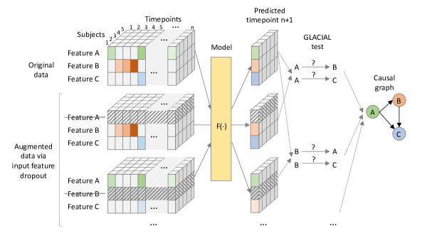
Figure 1: Overview of the proposed GLACIAL approach for longitudinal studies.

Constraint-based methods such as PC or FCI [50], which rely on independent samples and conditional independence tests, are also commonly used for causal discovery. These methods would use one observation per individual and thus is not designed to detect causal relationships reflected in temporal dynamics. Hence, we believe there is a lack of methods for causal discovery in longitudinal studies that consist of multiple individuals with sparse observations.

There are other issues that make causal discovery in longitudinal studies challenging. Longitudinal studies usually track multiple variables and the relationships between these variables may be nonlinear, which can be hard to detect. For instance, using linear GC to infer nonlinear relationships can be fast but may produce wrong results [27]. On the other hand, nonlinear GC methods (e.g. those based on non-parametric methods [53, 31]) do not scale to large number of variables [8]. Similarly, existing GC tests that use neural networks to infer nonlinear dynamics [54, 32, 24] also face scalability issues. Furthermore, when systems have a lot of variables, some variables may have many direct causes. In this case, regression-based GC [11, 28] often fails to detect some of the true causal relationships [46, 45, 58]. Another challenge of real-world longitudinal studies is missing data. While, there is no consensus about what to do about missing values [10], several works [52, 55] have tried to address this issue for cross-sectional data. Yet, as far as we know, missingness is under-explored in longitudinal studies, particularly in the context of causal discovery. Finally, GC, in its original form, does not differentiate between direct and indirect causes [58]. Although, in theory, infinite history (observations) could shield off indirect causes from being detected as edges in the output causal graph, when the number of observations per individual is small, false positives due to indirect causes is a common practical problem.

In this work, we propose GLACIAL (Figure 1), which stands for a “Granger and LeArning-based CausalIty Analysis for Longitudinal studies.” GLACIAL combines GC with a practical machine-learning based approach to test for causal relationships between multiple variables in a longitudinal study. GLACIAL extends GC to longitudinal studies by treating each individual’s trajectory as an independent sample, governed by a shared causal mechanism that is reflected in the temporal dynamics. Thus, by applying a standard train-test setup with hold-out individuals, GLACIAL can test for effects of causal relationships in expectation. GLACIAL leverages a single multi-task neural network, trained with input feature drop-out, to learn nonlinear relationships in time-varying data, while handling missing values. Thus, although neural networks have been used in the past for causal discovery, GLACIAL allows us to efficiently test for causal relationships in a large number of variables in real-world data where timepoints may be sampled irregularly and may contain missing values. Furthermore, GLACIAL also implements additional post-processing steps to account for indirect causes and resolve the directionality of detected ambiguous associations. Extensive experiments using both synthetic and real longitudinal data show that GLACIAL can infer relationships accurately even in challenging real-world scenarios with sparse observations, a large number of variables and direct causes, and a large degree of missing data.

2 Background

Most existing causal discovery (CD) methods are not intended for the longitudinal study design, where multiple individuals are sparsely observed at different timepoints. CD methods designed for timeseries data or independent samples are often used in the longitudinal setting even though this is may lead to bad performance.

Causal Discovery

CD methods intended for cross-sectional studies are ill-suited for longitudinal studies. They often fall under: constraint-based search (e.g. PC and FCI [50]), score-based search (e.g. GES [4]), functional causal models (FCMs, e.g. LiNGAM [49], ANM [15, 61], and PNL [60, 62]), or continuous optimization (e.g. NOTEARS [64]). Search methods can scale well if causal relationships are linear [23, 41] although their output may not be informative enough (e.g. contains bidirectional edges). In contrast, by making strong assumptions about the functional form of the causal process, FCM can better identify the causal direction [18, 63], although FCM methods usually do not scale well [10]. Besides, if the assumed FCM is too restrictive to be able to approximate the true data generating process, the results may be misleading.

There are also various CD methods for timeseries such as ANLTSM [5], PCMCI(+) [46, 44] (based on PC), tsFCI [9] and SVAR-(G)FCI [29, 30] (based on FCI), VAR-LiNGAM [19] (based on LiNGAM), TiMINo [38] (based on FCM), or DYNOTEARS [36] (based on NOTEARS). These methods take in consecutive blocks of observations and output a Full Time Graph [39], which contain not only the variables in the system but also their temporally-lagged versions. Although methods for timeseries may be better than cross-sectional ones, they are still not ideal for longitudinal data where sparse observations with potentially missing values come from more than one individual.

Granger Causality

GC [11, 12] checks for dependence between variables’ timeseries, after accounting for other available information. Temporal dependence is thus linked to causation by the “Common Cause Principle”: two dependent variables are causally related (one causes the other, or both share a common cause) [39]. Checking pairwise dependence in GC can be efficient, but often yields false positives because other variables in the system are not accounted for. In contrast, multivariate GC can account for common causes and therefore is more accurate but also more computationally demanding [7, 8]. In practice, multivariate GC may be infeasible for a large set of variables and more efficient approaches [1, 17] were developed to deal with this challenge. Recently, more general GC tests based on neural networks [54, 32, 24] have been proposed which outperform vector auto regressive (VAR) linear GC [10]. Scaling these neural-network based GC methods to handle a large number of variables is still a concern.

Missing data

For cross-sectional studies, missing values can be imputed, which may result in data contradicting the causal processes. Alternatively, observations with missing values can be removed (list-wise deletion), which can lead to the omission of vast amounts of valuable datapoints. Test-wise Deletion [52] (TDPC) is more data-efficient than list-wise deletion but may produce spurious edges when missingness is not completely at random [55]. MVPC [55] corrects TDPC’s output to account for different missingness scenarios. To our knowledge, no existing method addresses missingness for CD in longitudinal studies.

3 Method

Both cross-sectional CD methods (multiple individual, single timepoint data) and timeseries CD methods (single individual, multiple timepoints data) are ill-suited for longitudinal studies (multiple individuals, multiple timepoints data). Besides, prior methods often assume timeseries are infinitely long (i.e. unlimited history), regularly sampled, and without missing values. Thus, they may not work for real-world datasets when observation history per individual is limited, irregular, and riddled with missing values. Section 3.1 shows how GLACIAL handles longitudinal data. Section 3.2 shows how GLACIAL deals with irregularly sampled timepoints containing missing values. Section 3.3 shows GLACIAL’s post-processing strategies to account for limited history of observed timeseries.

3.1 Granger Causality Formulation

A popular GC test is based on comparing the mean squared error (MSE) achieved by two predictors [12]. Let $\mathbf{X}_{t}$ and $\mathbf{Y}_{t}$ be time-varying variables indexed with positive integer $t\in\{0,\ldots T-1\}=[T]$. We use super-script notation to indicate history: $\mathbf{X}^{t}=\{\mathbf{X}_{0},\ldots,\mathbf{X}_{t-1}\}$ . $\mathbf{\Omega}^{t}=\mathbf{X}^{t}\cup\mathbf{Y}^{t}\cup\dots$ is the union of all histories. In the GC MSE formulation, we conclude that “Y causes X” if:

$$\delta_{t}(X|Y) =\mathsf{MSE}(\mathbf{X}_{t},\mathbb{E}[\mathbf{X}_{t}|\mathbf{\Omega}^{t}\setminus\mathbf{Y}^{t}])$$

$$-\mathsf{MSE}(\mathbf{X}_{t},\mathbb{E}[\mathbf{X}_{t}|\mathbf{\Omega}^{t}])>0,\forall t\in[T]$$ (1)

where $\mathbb{E}$ denotes (conditional) expectations. Equation 1 simply calculates the MSE difference between two optimal (in an MSE sense) predictors of $X$ (also see [12] and Appendix A). The first predictor (i.e. $\mathbb{E}[\mathbf{X}_{t}|\mathbf{\Omega}^{t}\setminus\mathbf{Y}^{t}]$) is not given information about $Y$. The second predictor (i.e. $\mathbb{E}[\mathbf{X}_{t}|\mathbf{\Omega}^{t}]$) is given all past information including about $Y$. Since $\delta_{t}(X|Y)\geq 0,\forall t$, Equation 1 can be re-written:

$$\Delta\mathsf{MSE}(X|Y)=\mathbb{E}\Big{[}\frac{1}{T}\sum_{t=0}^{T-1}\delta_{t}(X|Y)\Big{]}>0$$ (2)

Section 3.2 details how this test can be done in practice when the optimal predictors are not given. We are particularly interested in the setting with multiple observed independent individual trajectories.

3.2 Choice of Predictor

We can approximate the MSE-optimal predictors with neural networks $F$ and $G$.

$$\delta_{t}(X|Y;F,G) =\mathsf{MSE}(\mathbf{X}_{t},F(\mathbf{X}_{t};\mathbf{\Omega}^{t}\setminus\mathbf{Y}^{t}))$$

$$-\mathsf{MSE}(\mathbf{X}_{t},G(\mathbf{X}_{t};\mathbf{\Omega}^{t}))$$ (3)

$$\Delta\mathsf{MSE}(X|Y;F,G) =\mathbb{E}\Big{[}\frac{1}{T}\sum_{t=1}^{T}\delta_{t}(X|Y;F,G)\Big{]}$$ (4)

To calculate $\delta_{t}(X|Y;F,G)$, we first have to train the neural networks using a training set. Once trained, the neural networks can be used to calculate $\Delta\mathsf{MSE}(X|Y;F,G)$ using hold-out test individuals. Thus, the predictors’ performance depends on the training data, optimization, network initialization, and other implementation details. Even with the best optimizer and initialization procedure, a bad training-test split of data could, for instance, result in sub-optimal network weights and consequently false causal relations prediction. For more robust causal discovery, in GLACIAL, we repeat the estimation of $\Delta\mathsf{MSE}(X|Y;F,G)$ multiple times using different random splits of data and test that $\Delta\mathsf{MSE}$ is positive on average using a statistical test.

We use a single recurrent neural network (RNN) [13] in place of all predictors. The RNN is trained to predict the next step values of all the variables given all available past values. In particular, the RNN model from [34] was used since it can impute missing values. Note that the choice of neural network architecture is not critical. Any architecture should work as long as it can handle missing data and learn from temporal dynamics to forecast future values.

Input Feature Dropout

Training separate neural networks to compute $\Delta\mathsf{MSE}(X|Y;F,G)$ for each variable pair would create a substantial burden for applying this approach to systems with large number of variables. This is because the number of networks required would be proportional to the number of variables squared. Instead, we propose to train a single multi-task (i.e., multi-output) RNN, $F(\cdot;\theta)$, to approximate $\mathbb{E}[\mathbf{X}_{t}|\mathbf{\Omega}^{t}\setminus\mathbf{Y}^{t}]$ and $\mathbb{E}[\mathbf{X}_{t}|\mathbf{\Omega}^{t}]$, for all predicted variables $\mathbf{X}_{t}$. The RNN acts as the former when $Y$ is masked out of the input vector and acts as the latter when the input is complete. To obtain a model that can produce accurate predictions under these scenarios, during training, we augment each mini-batch by dropping out individual variables from the input features.

Input: Data splits $D_{1},\dots,D_{n}$

Output: Causal graph $G$

// Step 1 - Association detection using the GC MSE test

1 for each data split $D_{i}$ do

2       Train RNN $F_{i}$ using training set of $D_{i}$

3       for each variable pair $(u,v)$ do

4             Calculate $\Delta$MSE(u, v)[i] using $F_{i}$ and test set of $D_{i}$

5      

6for each variable pair $(u,v)$ do

7       t-statistic, p-value = t-test($\Delta$MSE(u, v))

8       if p-value ¡ threshold then

9             Add edge $(u,v)$ to $G$;     E[u, v] = t-statistic

10      

11

// Step 2 - Orient bidirectional edges

12 for each pair of edges $(u,v)$ and $(v,u)$ in $G$ do

13       if $E[u,v]<E[v,u]$ then

             Remove edge $(u,v)$ from $G$

              // $v\rightarrow u$ has stronger effect

14            

15      else

             Remove edge $(v,u)$ from $G$

              // $u\rightarrow v$ has stronger effect

16            

17      

18

// Step 3 - Prune indirect causes

19 for each edge $(u,v)$ in $G$ do

20       for each path $p=(w_{1}=u,w_{2},\dots,w_{k}=v)$ from $u$ to $v$ do

21             if $E[u,v]<E[w_{j},w_{j+1}]\;$ for some $j$ then

22                   Remove edge $(u,v)$;     break

23            

24      for each path $p=(w_{1}=v,w_{2},\dots,w_{k}=u)$ from $v$ to $u$ do

25             if $E[u,v]<E[w_{j},w_{j+1}]\;$ for some $j$ then

26                   Remove edge $(u,v)$;     break

27            

28      

Algorithm 1 GLACIAL

Implementation Details

We used repeated 5-fold cross-validation to split a dataset into training, validation, and test sets with a 3:1:1 ratio. The RNN is trained to minimize next-step prediction error using Adam [25], L2 loss, and a learning rate of 3E-4. The RNN has one hidden layer of size 256. Training was done on a NVIDIA TITAN Xp GPU. The validation set is used for early stopping. Cross-validation is repeated 4 times, resulting in 20 different splits of data. We find 4 repetitions to strike a good balance between robustness and speed. Running more repetitions might slightly improve the results when missingness is severe but at a higher computational cost (see Appendix E). We perform a t-test on the $\Delta\mathsf{MSE}$ statistic and use the significance level threshold of 0.05.

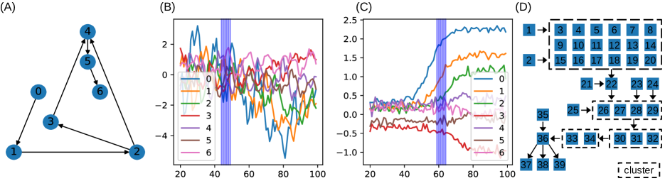
Figure 2: Simulated data. (A) Basic graph (7 nodes) that has all basic structures (chain, fork, collider). (B) Individual with random-walk trajectories (raw data before standardizing to zero mean and unit variance). Only timepoints at the vertical lines are observed. (C) Individual with sigmoid trajectories. (D) More realistic graph (39 nodes) that resembles the RTK/RAS signaling pathway. Nodes in the same cluster share the same causal relationships.

3.3 Post-Processing

GC assumes history of the timeseries is infinite. When observations are finite as in real-world longitudinal studies, GC may draw wrong conclusions. E.g., consider following deterministic system:

$$\textbf{Y}_{t} =a\textbf{Y}_{t-1}+b\textbf{Y}_{t-2}$$

$$\textbf{X}_{t} =c\textbf{Y}_{t-2}.$$

In this system, $Y$ causes $X$ since manipulating $Y$ will change the value of $X$. By the same logic, $X$ is not the cause of $Y$ because manipulating $X$ will not change $Y$.

When history is infinite, GC works as expected

$$\mathbb{E}[\mathbf{Y}_{t}|\mathbf{X}^{t},\mathbf{Y}^{t}]=\mathbb{E}[\mathbf{Y}_{t}|\mathbf{Y}^{t}]=\mathbf{Y}_{t}$$

$$\mathsf{MSE}(\mathbf{Y}_{t},\mathbb{E}[\mathbf{Y}_{t}|\mathbf{Y}^{t}])=\mathsf{MSE}(\mathbf{Y}_{t},\mathbb{E}[\mathbf{Y}_{t}|\mathbf{X}^{t},\mathbf{Y}^{t}])=0$$

$$\Rightarrow X\;\text{does not cause}\;Y\quad\text{(correct)}$$

However, when only 1 past observation is given (finite history), GC reaches the wrong conclusion

$$\mathsf{MSE}(\mathbf{Y}_{t},\mathbb{E}[\mathbf{Y}_{t}|\mathbf{Y}_{t-1}])\geq\mathsf{MSE}(\mathbf{Y}_{t},\mathbb{E}[\mathbf{Y}_{t}|c\mathbf{Y}_{t-2},\mathbf{Y}_{t-1}])$$

$$\geq\mathsf{MSE}(\mathbf{Y}_{t},\mathbb{E}[\mathbf{Y}_{t}|\mathbf{X}_{t-1},\mathbf{Y}_{t-1}])$$

$$\Rightarrow X\;\text{causes}\;Y\quad\text{(incorrect)}$$

Thus, GC may detect edges in both direction ($X\rightarrow Y$ and $Y\rightarrow X$) for a pair of variables when limited history is given. It can be shown in a similar fashion that if $X$ causes $Y$ and $Y$ causes $Z$ ($X$ is the indirect cause of $Z$), $Y$ will not be able to shield $Z$ from $X$ if only limited history is given. Thus, GC will also detect edges for indirect causes in both direction ($X\rightarrow Z$ and $Z\rightarrow X$).

In GLACIAL, we implement two additional post-processing steps to remove these false positives. Let $E(X|Y)$ be the statistic (e.g. the t-test) that tests for the positivity of $\Delta\mathsf{MSE}$ from several train/test splits. Thus $E(X|Y)$ can be viewed as a test for whether $Y$ causes $X$.

1. Orient bidirectional edge

If $E(X|Y)<E(Y|X)$ remove $Y\rightarrow X$, else remove $X\rightarrow Y$. This step is similar to prior work such as [15, 61, 22, 26] which leverages causal asymmetry to determine the causal direction (the direction with the bigger effect is regarded as the causal direction). T-statistic has been shown to be informative for causal discovery [57].

2. Remove indirect edge

For an edge $X\rightarrow Y$, remove $X\rightarrow Y$ if either

• There exists edge $U\rightarrow V$ on an alternative path from $X$ to $Y$ such that $E(Y|X)<E(V|U)$

• There exists edge $U\rightarrow V$ on an alternative path from $Y$ to $X$ such that $E(Y|X)<E(V|U)$

Intuitively, if the effect of $X\rightarrow Y$ is smaller than that of any edge on an alternative path, then $X$ is likely an indirect cause of $Y$. A complete description of GLACIAL is shown in Algorithm 1. Ablation in Appendix C shows the contribution of these two post-processing steps.

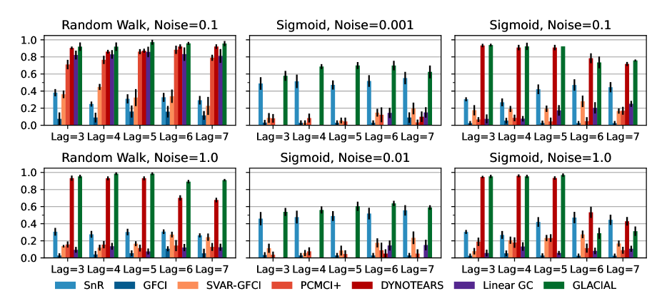
Figure 3: Average F1-scores at different lag-time and measurement noise for 7-node graph. GLACIAL outperforms baselines in most settings of sample path, lag-time, and measurement noise.

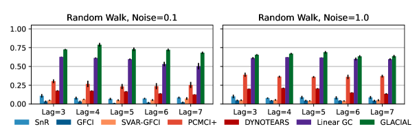
Figure 4: Average F1-scores at different lag-time and measurement noise for 39-node graph (Gaussian random-walk). GLACIAL outperforms baselines in most settings of lag-time and measurement noise.

4 Experimental Set-up

4.1 Baselines

We benchmark GLACIAL against both CD methods for cross-sectional data and CD methods for timeseries.

CD Methods for Cross-Sectional Data

We compare against GFCI [35] and Sort-N-Regress [42] (SnR). GFCI is a competitive algorithm for cross-sectional data that combines GES and FCI. SnR is a simple baseline to ensure that benchmarked approaches go beyond exploiting differences in variables’ marginal variance [42]. As these approaches assume independent observations, only first timepoints (observations) of individuals are used. In most longitudinal studies, individuals are guaranteed to have first timepoints (but not other timepoints). Hence, using the first timepoints will result in the most number of independent timepoints with the least amount of missing data in real-world datasets. Besides, using all timepoints led to worse performance in our preliminary experiments using simulated data. Similar to [48], GFCI is run multiple times (i.e. 20) using different bootstraps of subjects’ first timepoints, resulting in multiple graphs. Only edges appearing in more than half of the resultant graphs are kept in final graph. A higher threshold (80%) led to worse result (see Appendix F).

CD Methods for Timeseries Data

We also adopt linear GC, SVAR-GFCI [30], PCMCI+ [44], and DYNOTEARS [36] as baselines. For linear GC, F-statistic was used to test for presence of edges using the same threshold as in GLACIAL. For longitudinal data, one could either (1) estimate one causal graph for each individual and aggregate the graphs or (2) estimate just one graph using concatenated data from all the individuals. Since (1) often fails when the number of timepoints per individual is sparse, (2) was used instead. Causal discovery using concatenated individuals’ data has been investigated in [6, 40]. Besides, linear GC could output false positives when timeseries are non-stationary [14]. One could make the timeseries stationary by calculating the difference or the log difference between timepoints [51]. However, using differences led to worse results in our experiments so we report the results using the original timeseries instead.

The input to SVAR-GFCI and PCMCI+ are also the concatenated timeseries from all the individuals. For DYNOTEARS which can accept timeseries from multiple individuals, the timeseries are not concatenated. The hyper-parameters of SVAR-GFCI, PCMCI+, and DYNOTEARS are selected based on the suggestions in their original publications.

Missing data

For data with missingness, TDPC [52] and MVPC [55] are used instead of GFCI. For a dataset, each algorithm is run 20 times and the results are aggregated using the same 50% threshold. As far as we know, there is no prior work on applying causal discovery methods to timeseries data with missing values. Therefore, we used linear interpolation to fill out missing values in the data before applying these methods (linear GC, SVAR-GFCI, PCMCI+, and DYNOTEARS). It may not be feasible to apply more complex interpolation methods due to the limited number of timepoints (especially after discounting missing values).

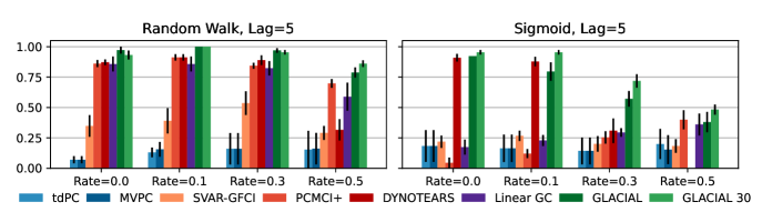
Figure 5: Average F1-scores at various levels of missing at random. Lag-time=5. Noise level = 0.1. GLACIAL outperforms baselines in most settings. Running GLACIAL for more repetitions (i.e. 30 instead of 4, denoted as GLACIAL 30; see Section 3.2) can improve F1-scores when missing values are present in data.

4.2 Simulated Data

The sample size in the simulations was set to 2000 individuals, roughly the size of the ADNI dataset (see Section 4.3). Only six timepoints are extracted from each individual’s timeseries to simulate sparse observations (see Appendix D for results with 24 timepoints). We consider two scenarios. First, the temporal dynamics are parameterized via the sigmoid function, which is a widely used model for the trajectories of biomarkers, e.g., in Alzheimer’s disease [21]. In the second scenario, we implement random-walk series. See Appendix B for further details. As causal structure of simulated data may leak through variables’ marginal variance, the data are standardized to zero-mean and unit-variance to prevent CD algorithms from gaming the simulated data [42].

Figure 2 shows the causal graphs used for generating the synthetic data. The first graph (7 nodes) contains all the basic structures, namely chain, fork, and collider. The second graph (39 nodes) is used to demonstrate GLACIAL’s scalability. This graph is inspired by the RTK/RAS signaling pathway in oncology and is taken from [47]. The second graph is a realistic target that a causal discovery algorithm should be able to find from observational data. Since the shape of the evolution of signaling proteins is not known, we use Gaussian random-walk as the sample path function. To simulate missingness (completely at random), the values for each timeseries of an individual are independently dropped at fixed rate $p\in\{0.1,0.3,0.5\}$. Since values from different timeseries are dropped independently, the resulted data could contain individuals with all timepoints having at least one missing values.

4.3 Real-world Data from an Alzheimer’s Disease Study

We use ADNI [20], a longitudinal study of Alzheimer’s disease (AD) and consists of 1789 individuals. Each individual in ADNI has about 7 timepoints on average. The ADNI study tracks multiple AD biomarkers such as region-of-interest (ROI) volumes (e.g. hippocampal) derived from structural MRI scans, cognitive tests (e.g. ADAS13), proteins (e.g. amyloid beta) derived from cerebral spinal fluid samples, and molecular imaging that captures the brain’s metabolism (e.g. FDG PET). The missingness rates vary for different biomarkers, ranging from $30\%$ (ADAS13) to around $80\%$ (FDG PET). The variables used are shown in Figure 6(c) and described in detail in Appendix G.

4.4 Metrics

F1-score, which is the harmonic mean of precision and recall, is used to quantify different approaches’ performance. Note that we assume that there is a ground-truth (directed) graph that describes causal relationships. Each method will also return a list of directed edges between variables. Precision is the ratio of correctly identified edges over all predicted edges, while recall is the ratio of correct edges over all ground-truth edges. A predicted edge is considered incorrect if the edge does not exist in the ground-truth graph or the predicted direction contradicts the ground-truth direction. Thus, a predicted bidirectional edge would be incorrect if the ground-truth edge has only one direction.

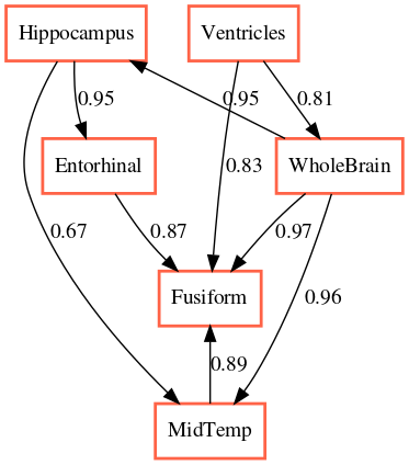
(a) Only ROI volumes

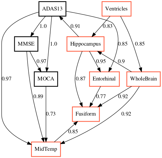
(b) ROI volumes and cognitive tests

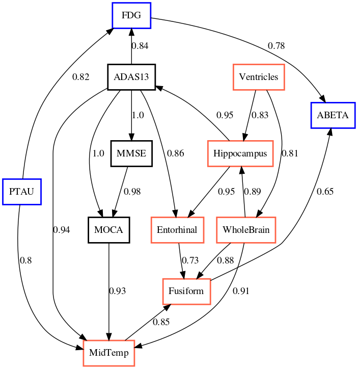
(c) Extend set of variables

Figure 6: GLACIAL’s predicted interaction of ADNI biomarkers. ROI volumes are in red, cognitive tests are in black, and the rest are in blue. ABETA: amyloid beta, PTAU: phosphorylated tau. Edge weights are frequencies at which edges were detected in multiple runs.

5 Experimental Results

5.1 Simulated Data

7-node graph

For random-walk data, GLACIAL outperforms the baselines for various lag-times and measurement noise levels (Figure 3, 1st column). Similarly, GLACIAL also outperforms the baselines, for the sigmoid data (2nd and 3rd column). GLACIAL’s performance dips (3rd column) when input history (5 years) is shorter than the lag-time (6 or 7 years). This dip is more pronounced when measurement noise is high (3rd column, bottom).

DYNOTEARS fails to detect causal relations in systems with almost deterministic dynamics (2nd column) even though it is the best baseline. System with deterministic dynamics is also challenging for linear GC [39] and SVAR-GFCI although they are slightly better than DYNOTEARS (F1-score $<$ 0.2). Interestingly, GLACIAL still works in these systems (F1-score = 0.6). Only GLACIAL manages to consistenly beat the strong SnR (Sort-N-Regress) baseline, demonstrating the proposed method’s strength.

39-node graph

Even though DYNOTEARS is the best baseline for the 7-node graph, its performance on the big graph is worse than linear Granger (Figure 4). GLACIAL consistently outperforms all baselines on this big graph when the sample path is Gaussian random-walk. GLACIAL performs quite well despite the presence of a cluster of direct causes whose contribution to the node “22” may be too small to be detected.

Missing data

Figure 5 shows the F1-scores of various approaches at different degrees of missingness. GLACIAL outperforms TDPC and MVPC, CD approaches tailored for missing data, by better exploiting the temporal dynamics within individuals’ timeseries. GLACIAL also outperforms CD methods for timeseries such as PCMCI+ and DYNOTEARS. DYNOTEARS is competitive when missingness level is low but often fails when the missingness level is high. PCMCI+ does well for random walk timeseries at various missingness levels (left panel) but fails for sigmoid timeries (right panel). When half of the values are missing (Rate=0.5), GLACIAL can still infer some causal relationships in the system. As an aside, GLACIAL’s performance on missing data can be improved with more repetitions (see ablation in Appendix E).

5.2 Results on ADNI Data

The output of applying GLACIAL to different sets of ADNI biomarkers are shown in Figure 6. Edge weights denote the frequencies at which edges were detected in multiple runs. Most of the edges are consistently detected across different runs with the exception of “Hippocampus $\rightarrow$ MidTemp” (67%, Figure 6(a)) and “Fusiform $\rightarrow$ ABETA” (65%, Figure 6(c)). There is a high degree of agreement between the 3 graphs which all show the “Ventricle” is a source in the causal graph and “Fusiform” is at the end of the chain. The presence of the edge “Hippocampus $\rightarrow$ Entorhinal” is also consistent with literature. In comparison, baselines’ outputs are less interpretable (see Appendix G). The outputs of PCMCI+, DYNOTEARS, and linear Granger contain hardly any edge between ROI volumes while SVAR-GFCI’s output has many bidirectional edges.

6 Discussion

In a longitudinal study, multiple individuals are followed and sparsely observed for a limited number of times. Longitudinal studies commonly track many variables, which are likely governed by nonlinear dynamics that might have individual-specific idiosyncrasies. Longitudinal studies are particularly common in population health applications. Yet, longitudinal studies are not amenable to the popular Granger causality (GC) analysis, since GC was developed to analyze a single multivariate densely sampled timeseries. Furthermore, real-world longitudinal data often suffer from widespread missingness. We developed GLACIAL which combines the GC framework with a machine learning based prediction model to address this need. GLACIAL treats individuals as independent samples and uses average prediction accuracy on hold-out individuals to test for causal relationships.

GLACIAL exploits a single multi-task neural network trained with input feature dropout to efficiently probe links. GLACIAL places no restriction on the design of the neural network predictor. This flexibility allows future extensions of our work. For example, Transformers [56] or Neural ODEs [3] can be used instead of the RNN architecture.

Limitations and Future Work

Although we have shown that GLACIAL works in a range of settings, such as variable lag-times, measurement noise levels, and degree of missingness, there are still some areas that need more investigation. In this work, we focused on real-valued variables since they are the most common. However, extending GLACIAL to discrete variables by adopting techniques in [37, 2, 16] would make it applicable to an even wider range of tasks. Besides, GLACIAL assumes that causal relationships form a DAG without feedback and instantaneous effects. We leave these problems for future work.

Acknowledgements

This work was supported by NIH grants R01LM012719, R01AG053949, the NSF NeuroNex grant 1707312, and the NSF CAREER 1748377 grant (MS). Data collection and sharing for this project was funded by the Alzheimer’s Disease Neuroimaging Initiative (ADNI) (National Institutes of Health Grant U01 AG024904) and DOD ADNI (Department of Defense award number W81XWH-12-2-0012).

Appendix A Granger Causality MSE test

Let $\mathbf{X}_{t}$ and $\mathbf{Y}_{t}$ denote time-varying random variables (stochastic processes), discretely indexed with positive $t\in[T]=\{0,\ldots,T-1\}$. Let’s use super-scripts to denote the history: $\mathbf{X}^{t}=\{\mathbf{X}_{0},\ldots...\mathbf{X}_{t-1}\}$. We will use $\mathbf{\Omega}^{t}=\mathbf{X}^{t}\cup\mathbf{Y}^{t}\cup\dots$ to indicate the union of all sets of historical variables available at time $t$. The general GC hypothesis is:

$$Y\;\text{causing}\;X\Rightarrow\exists\text{ some event $A$}\text{ and }t\in[T]\text{ such that}\Pr(\mathbf{X}_{t}\in A|\mathbf{\Omega}^{t})\neq\Pr(\mathbf{X}_{t}\in A|\mathbf{\Omega}^{t}\setminus\mathbf{Y}^{t})$$

Equivalently, we have:

$$\Pr(\mathbf{X}_{t}|\mathbf{\Omega}^{t})=\Pr(\mathbf{X}_{t}|\mathbf{\Omega}^{t}\setminus\mathbf{Y}^{t}),\forall t\in[T]\Rightarrow Y\;\text{does not cause}\;X$$

In general it is not possible to compare these conditional probabilities based on observed timeseries data. A practical approach is to compare conditional expectations:

$$\mathbb{E}[\mathbf{X}_{t}|\mathbf{\Omega}^{t}]\stackrel{{\scriptstyle?}}{{=}}\mathbb{E}[\mathbf{X}_{t}|\mathbf{\Omega}^{t}\setminus\mathbf{Y}^{t}].$$

Note that conditional expectations can be infeasible to compare, so we often need further assumptions. One observation is that the conditional expectation is the optimal estimator that minimizes the mean square error (MSE). This gives rise to a GC test that compares the MSE of least-squares predictors. In this approach, we conclude that “$Y$ causes $X$” if:

$$\mathsf{MSE}(\mathbf{X}_{t},\mathbb{E}[\mathbf{X}_{t}|\mathbf{\Omega}^{t}])<\mathsf{MSE}(\mathbf{X}_{t},\mathbb{E}[\mathbf{X}_{t}|\mathbf{\Omega}^{t}\setminus\mathbf{Y}^{t}])$$ (5)

Note that, in above equation the right hand side is larger than or equal to the left hand side because, in general, the least-square loss will be smaller with more history.

In practice, implementation of the GC MSE test often relies on two more assumptions. The first is the stationarity assumption. That is, we suppose $\mathbb{E}[\mathbf{X}_{t}|\mathbf{\Omega}^{t}]$ and $\mathbb{E}[\mathbf{X}_{t}|\mathbf{\Omega}^{t}\setminus\mathbf{Y}^{t}]$ are independent of $t$. Second, we assume the stochastic processes are Markovian and thus a finite history (often just the prior timepoint) is sufficient for making the least-square forecast. In our framework, the Markovian assumption can be relaxed because the RNN forecast model can digest all available history.

Appendix B Pseudo-code for Data Generation

Algorithm 2 shows the steps to generate data from a given causal graph $G$. First, the edge weights are sampled. Then, for each individual, the timeseries are generated in topological order. If a node has no parent, i.e., if it is a source node, its timeseries is specified by the sample path $f$ (Gaussian random-walk or sigmoid). The random-walk function is a conventional choice while the sigmoid function yields trajectories that mimic the evolution of many real-world dynamic systems [21]. A non-source node’s timeseries is the weighted sum of the lagged version of its parents’ timeseries. Next, Gaussian measurement noise with standard deviation $\sigma$ is added to the timeseries. Finally, a discrete set of timepoints within a randomly-chosen observation window are extracted, mimicking a real-world longitudinal study.

• Gaussian random-walk: $f(t)=\sum_{i=0}^{t}\mathcal{N}(0,1)$

• Sigmoid: $f(t)=\frac{A}{1+e^{-k(t-t_{0})}};\quad A\sim\mathsf{Unif}(1,2),\;t_{0}\sim\mathsf{Unif}(40,60),\;k\sim\mathsf{Unif}(0.1,0.3)$

For random-walk timeseries, the noise variance $\sigma$ is either 0.1 or 1.0 (smaller $\sigma$ has no visible effect). For sigmoid timeseries, $\sigma=0.001,0.01,0.1,1.0$. Since measurement noise can (1) induce spurious causality between unrelated variables and (2) suppress true causality [33, 10], it is important to benchmark across different levels of measurement noise. For each set of parameters ($f$, lag-time $L$, and $\sigma$), we generated 5 different randomized datasets so as to estimate the standard error of the performance metrics.

Input: Causal graph $G$, sample path $f$, number of individuals $n$, number of timepoints $m$,

Lag-time $L$, measurement noise magnitude $\sigma$

Output: Dataset $D=(X_{1},\dots,X_{n})$

1

// Sample edge weights

2 for each edge $(u,v)\in G$ do

3       $s_{uv}\sim\mathsf{Rademacher}();\quad\quad m_{uv}\sim\mathsf{Unif}(0.5,1);\quad\quad w_{uv}=s_{uv}*m_{uv}$

4

// Sample observation series of an individual

5 for each individual $i$ do

6       for each node $v$ do

             $b\sim\mathsf{Unif}(-0.5,0.5)$

              // bias term

7             if $v$ has no parent then

                   $s_{v}[t]=b+f[t]$

                    // time $t\in[0,100]$

8                  

9            else

10                   $s_{v}[t]=b+\sum_{u,(u,v)\in G}w_{uv}*s_{u}[t-L]$

            $s_{v}[t]=s_{v}[t]+\mathcal{N}(0,\sigma)$

              // measurement noise

11            

      $S_{i}=\{s_{u},u\in G\}$

        // individual data

       $t_{\text{start}}\sim\mathsf{Unif}(30,70);\quad\quad t_{\text{end}}=t_{\text{start}}+m$

        // observation window

       $X_{i}=S_{i}[t_{\text{start}}:t_{\text{start}}]$

        // extract timepoints within window

12      

Algorithm 2 Data Generation

Appendix C Ablation of GLACIAL

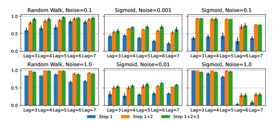
Figure 7: Contribution from different steps of GLACIAL to F1-scores (7-node graph simulation).

GLACIAL’s first step tests for edges in the causal graph by comparing the difference in MSE on hold-out subjects. However, when test subjects are only sparsely observed for a limited number of times, this step may find spurious edges (edges from effect to cause or edges between indirect cause, e.g. a grand-parent, and effect). To address this problem, GLACIAL has two additional steps: one (Step 2) to remove edges from effect to cause and another (Step 3) to prune edges between indirect cause and effect. Figure 7 shows the contribution of these two post-processing steps to F1-scores at various lag-time and noise level (7-node graph simulation). In all scenarios, including Step 2 consistently leads to better result. When the observation noise is low ($\sigma<1$), including Step 3 leads to higher F1-score.

Appendix D Result with More Densely Sampled Data

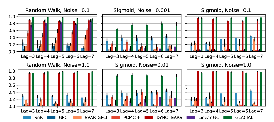
Figure 8: Average F1-scores at different lag-time and observation noise for 7-node graph. Each individual has 24 timepoints. GLACIAL outperforms baselines in all settings of sample path, lag-time, and observation noise.

In Section 5.1, each individual only has 6 timepoints (sparse observations) so linear GC did not work well. Thus, we investigated a scenario more favorable for linear GC where for when individuals have more timepoints (i.e. 24 timepoints). With more timepoints, linear GC results improve slightly but are still worse than that of GLACIAL (Figure 8). Additionally, using GC to estimate one causal graph for each individual could not find the correct graph even with 24 timepoints (hence, result not reported).

Appendix E GLACIAL’s Results with More Repetitions

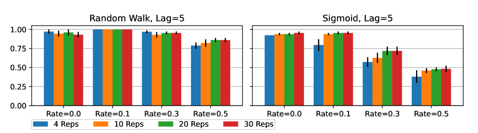
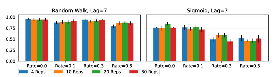
Figure 9: More repetitions of cross-validation lead to slightly better result at the expense of running time. Top panels: Lag-time (L) = 5. Bottom panels: Lag-time (L) = 7

GLACIAL’s results in Section 5.1 were obtained by repeating 5-fold cross-validation for 4 times. Increasing the number of repetitions leads to higher F-1 score as shown by the trend in Figure 9. However, the gap between 10 repetitions and 4 repetitions is not large enough to justify the extra computational cost of repeating more than 4 times in Section 5.1. Another interesting trend in Figure 9 is that the gap between 4 repetitions and 30 repetitions is more apparent for missing data. Thus, when the data is noisy (more missing values), more repetitions may yield more accurate results.

Appendix F Constraint-based Baselines with Higher Threshold

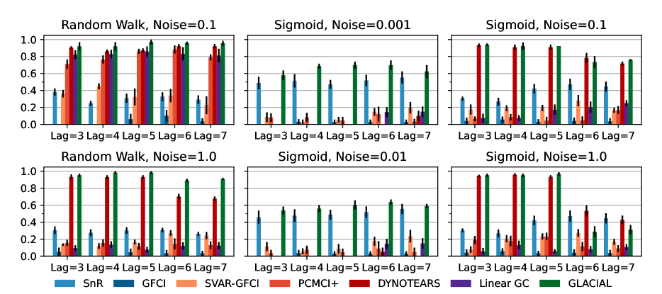
Figure 10: Performance of PC, GFCI, and FGES when cut-off threshold is set at 0.8 (80%).

The PC, GFCI, and FGES baselines are run multiple times using different data bootstraps, resulting in multiple graphs. To combine the graphs, we only retain edges that appear more than half of the runs. This procedure is similar to [48] although they used a more conservative threshold (0.8) in their work. Figure 10 shows the results of the constraint-based baselines when the threshold of 0.8 (80%) is used. Compared to the results in Figure 3, this more conservative threshold led to worse performance in the baselines.

Appendix G Experiment on ADNI Dataset

Description of ADNI Variables

Table 1: ADNI variables used for causal discovery.

Variable	Description	Data Modality
ABETA	Amyloid beta	Cerebral spinal fluid
FDG	Fluorodeoxyglucose PET	PET imaging
PTAU	Phosphorylated tau	Cerebral spinal fluid
ADAS13	ADAS-Cog13	Cognitive test
MMSE	Mini-Mental State Examination	Cognitive test
MOCA	Montreal Cognitive Assessment	Cognitive test
Entorhinal	Entorhinal cortical volume	MRI imaging
Fusiform	Fusiform cortical volume	MRI imaging
Hippocampus	Hippocampus volume	MRI imaging
MidTemp	Middle temporal cortical volume	MRI imaging
Ventricles	Ventricles volume	MRI imaging
WholeBrain	Whole brain volume	MRI imaging

Table 1 shows the ADNI variables used and how they were measured (Data Modality). These variables are complementary in what they measure. “ABETA” and “PTAU” measure the level of two proteins in cerebral spinal fluid that are indicative of Alzheimer’s disease. “FDG” measures brain cells’ metabolism while cognitive tests measure performance in various areas such as general cognition, memory, language et cetera. The quantitative variables derived from structural MRI scans (e.g. Hippocampus Volume) is often considered as a proxy of regional brain atrophy, or tissue loss linked to aging and/or neuro-degenerative processes.

We normalized the volumetric variables of each individual by dividing the measurements by the individual’s intracranial volume, or total head size, which is typically constant in adulthood. This is a standard normalization done to account for inter-individual variability in head sizes. FDG is a standardized uptake value ratio computed by dividing the average PET signal in an Alzheimer implicated region of interest to the signal in a control reference region. The Cerebral Spinal fluid markers correlate with the accumulation of the two Alzheimer’s associated pathologial proteins in the brain, namely tau tangles and amyloid plaque.

Interpretation of ADNI Causal Graphs

The order of the volumetric variables in Figure 6(a), 6(b), and 6(c) are mostly consistent with each other and prior literature on neuroimaging in aging and Alzheimer’s disease, where the size of ventricles and whole brain are earliest MRI markers of aging, and Alzheimer’s associated atrophy starts at the hippocampus, from where it spreads to cortical areas such as entorhinal and fusiform.The causal chains that appear in all three graphs are:

• “Ventricles” $\rightarrow$ “WholeBrain” $\rightarrow$ “Hippocampus” $\rightarrow$ “Entorhinal” $\rightarrow$ “Fusiform”

• “Ventricles” $\rightarrow$ “WholeBrain” $\rightarrow$ “MidTemp” $\rightarrow$ “Fusiform”

The ordering of cognitive tests are also consistent across all graphs. When we examine the ordering of variables from different data modalities, the causal chain of “Hippocampus” $\rightarrow$ “ADAS13” $\rightarrow$ “MMSE” $\rightarrow$ “MOCA” is quite interesting. This implies that the atrophy of the hippocampus, a brain region that plays a central role in memory and learning, leads to worse performance in tasks measured by cognitive tests. The relationship between MMSE and ADAS13 is surprising and deserves follow-up investigation, because classically MMSE is thought of as the earlier marker of cognitive impairment and ADAS13 is a measure of symptoms that appear later in Alzheimer’s disease. That said, to our knowledge, we are not aware of a study that examines the relationships between the temporal dynamics of these test scores. Our results indicate that changes in ADAS13 might foreshadow changes in MMSE.

Figure 11 shows the outputs of the baselines CD methods on the ADNI data. Linear interpolation was used to fill out missing values in the data. The outputs from PCMCI+, DYNOTEARS, and linear Granger are not very informative as they do not contain any edge between the ROIs. Although somewhat similar GLACIAL’s output, output from SVAR-GFCI has a lot of bidirectional edges. One of the possible reason for the seemingly worse performance of the baselines is the high missing rate in the ADNI data.

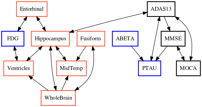
(a) SVAR-GFCI

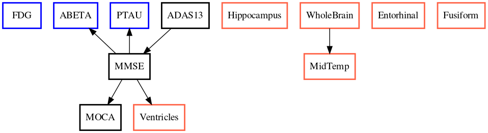
(b) PCMCI+

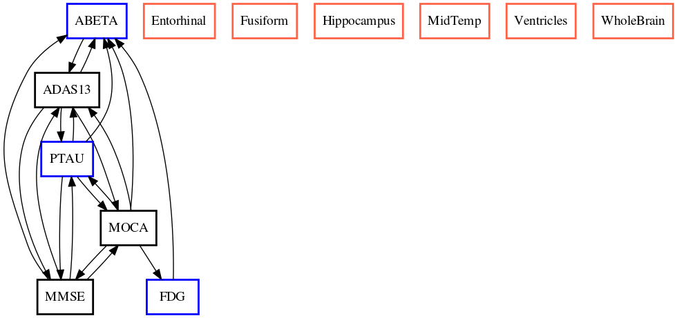
(c) DYNOTEARS

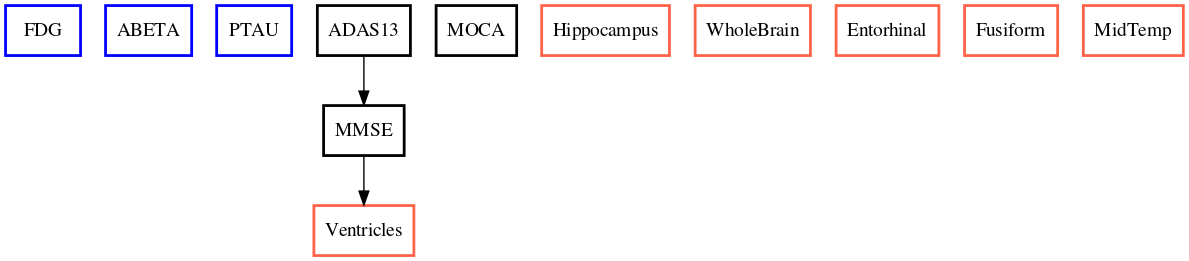
(d) Linear Granger

Figure 11: Baseline methods’ predicted interaction of ADNI biomarkers. ROI volumes are in red, cognitive tests are in black, and the rest are in blue. ABETA: amyloid beta, PTAU: phosphorylated tau.

References

- [1] S. Basu, A. Shojaie, and G. Michailidis. Network granger causality with inherent grouping structure. JMLR, 16(1):417–453, 2015.
- [2] R. Cai, J. Qiao, K. Zhang, Z. Zhang, and Z. Hao. Causal discovery from discrete data using hidden compact representation. In Proceedings of NIPS, 2018.
- [3] R. T. Chen, Y. Rubanova, J. Bettencourt, and D. K. Duvenaud. Neural ordinary differential equations. In Proceedings of NIPS, 2018.
- [4] D. M. Chickering. Optimal structure identification with greedy search. JMLR, 3(Nov):507–554, 2002.
- [5] T. Chu, C. Glymour, and G. Ridgeway. Search for additive nonlinear time series causal models. JMLR, 9(5), 2008.
- [6] X. Di, M. Wölfer, M. Amend, H. Wehrl, T. M. Ionescu, B. J. Pichler, B. B. Biswal, and A. D. N. Initiative. Interregional causal influences of brain metabolic activity reveal the spread of aging effects during normal aging. Human brain mapping, 40(16):4657–4668, 2019.
- [7] M. Eichler. Granger causality and path diagrams for multivariate time series. Journal of Econometrics, 137(2):334–353, 2007.
- [8] M. Eichler. Causal inference in time series analysis. Causality: Statistical Perspectives and Applications, pages 327–354, 2012.
- [9] D. Entner and P. O. Hoyer. On causal discovery from time series data using fci. Probabilistic graphical models, pages 121–128, 2010.
- [10] C. Glymour, K. Zhang, and P. Spirtes. Review of causal discovery methods based on graphical models. Frontiers in Genetics, 10:524, 2019.
- [11] C. Granger. Investigating causal relations by econometric models and cross-spectral methods. Econometrica, pages 424–438, 1969.
- [12] C. W. Granger. Testing for causality: A personal viewpoint. Journal of Economic Dynamics and control, 2:329–352, 1980.
- [13] A. Graves, M. Liwicki, S. Fernández, R. Bertolami, H. Bunke, and J. Schmidhuber. A novel connectionist system for unconstrained handwriting recognition. IEEE transactions on pattern analysis and machine intelligence, 31(5), 2009.
- [14] Z. He and K. Maekawa. On spurious granger causality. Economics Letters, 73(3):307–313, 2001.
- [15] P. Hoyer, D. Janzing, J. M. Mooij, J. Peters, and B. Schölkopf. Nonlinear causal discovery with additive noise models. Proceedings of NIPS, 21, 2008.
- [16] B. Huang, K. Zhang, Y. Lin, B. Schölkopf, and C. Glymour. Generalized score functions for causal discovery. In Proceedings of KDD, pages 1551–1560, 2018.
- [17] Y. Huang and S. Kleinberg. Fast and accurate causal inference from time series data. In The twenty-eighth international flairs conference, 2015.
- [18] A. Hyvärinen and P. Pajunen. Nonlinear independent component analysis: Existence and uniqueness results. Neural networks, 12(3):429–439, 1999.
- [19] A. Hyvärinen, K. Zhang, S. Shimizu, and P. O. Hoyer. Estimation of a structural vector autoregression model using non-gaussianity. JMLR, 11(5), 2010.
- [20] C. R. Jack Jr, M. A. Bernstein, N. C. Fox, P. Thompson, G. Alexander, D. Harvey, B. Borowski, P. J. Britson, J. L. Whitwell, C. Ward, et al. The alzheimer’s disease neuroimaging initiative (adni): Mri methods. Journal of Magnetic Resonance Imaging: An Official Journal of the International Society for Magnetic Resonance in Medicine, 27(4):685–691, 2008.
- [21] C. R. Jack Jr, D. S. Knopman, W. J. Jagust, R. C. Petersen, M. W. Weiner, P. S. Aisen, L. M. Shaw, P. Vemuri, H. J. Wiste, S. D. Weigand, et al. Tracking pathophysiological processes in alzheimer’s disease: an updated hypothetical model of dynamic biomarkers. The Lancet Neurology, 12(2):207–216, 2013.
- [22] D. Janzing, J. Mooij, K. Zhang, J. Lemeire, J. Zscheischler, P. Daniušis, B. Steudel, and B. Schölkopf. Information-geometric approach to inferring causal directions. Artificial Intelligence, 182:1–31, 2012.
- [23] M. Kalisch and P. Bühlman. Estimating high-dimensional directed acyclic graphs with the pc-algorithm. JMLR, 8(3), 2007.
- [24] S. Khanna and V. Y. Tan. Economy statistical recurrent units for inferring nonlinear granger causality. In Proceedings of ICLR, 2020.
- [25] D. P. Kingma and J. Ba. Adam: A Method for Stochastic Optimization. In Proceedings of ICLR, 2014.
- [26] M. Kocaoglu, A. G. Dimakis, S. Vishwanath, and B. Hassibi. Entropic causal inference. In Proceedings of AAAI, 2017.
- [27] S. Li, Y. Xiao, D. Zhou, and D. Cai. Causal inference in nonlinear systems: Granger causality versus time-delayed mutual information. Physical Review E, 97(5):052216, 2018.
- [28] H. Lütkepohl. New introduction to multiple time series analysis. Springer Science & Business Media, 2005.
- [29] D. Malinsky and P. Spirtes. Causal structure learning from multivariate time series in settings with unmeasured confounding. In ACM SIGKDD workshop on causal discovery, pages 23–47, 2018.
- [30] D. Malinsky and P. Spirtes. Learning the structure of a nonstationary vector autoregression. In Proceedings of AISTATS, pages 2986–2994, 2019.
- [31] D. Marinazzo, M. Pellicoro, and S. Stramaglia. Kernel method for nonlinear granger causality. Physical review letters, 100(14):144103, 2008.
- [32] M. Nauta, D. Bucur, and C. Seifert. Causal discovery with attention-based convolutional neural networks. Machine Learning and Knowledge Extraction, 1(1):312–340, 2019.
- [33] P. Newbold. Feedback induced by measurement errors. International Economic Review, pages 787–791, 1978.
- [34] M. Nguyen, T. He, L. An, D. C. Alexander, J. Feng, B. T. Yeo, A. D. N. Initiative, et al. Predicting alzheimer’s disease progression using deep recurrent neural networks. NeuroImage, 2020.
- [35] J. M. Ogarrio, P. Spirtes, and J. Ramsey. A hybrid causal search algorithm for latent variable models. In Conference on probabilistic graphical models, pages 368–379, 2016.
- [36] R. Pamfil, N. Sriwattanaworachai, S. Desai, P. Pilgerstorfer, K. Georgatzis, P. Beaumont, and B. Aragam. Dynotears: Structure learning from time-series data. In Proceedings of AISTATS, pages 1595–1605, 2020.
- [37] J. Peters, D. Janzing, and B. Schölkopf. Identifying cause and effect on discrete data using additive noise models. In Proceedings of AISTATS, pages 597–604, 2010.
- [38] J. Peters, D. Janzing, and B. Schölkopf. Causal inference on time series using restricted structural equation models. Proceedings of NIPS, 26, 2013.
- [39] J. Peters, D. Janzing, and B. Schölkopf. Elements of causal inference: foundations and learning algorithms. The MIT Press, 2017.
- [40] Z. Qing, F. Chen, J. Lu, P. Lv, W. Li, X. Liang, M. Wang, Z. Wang, X. Zhang, B. Zhang, et al. Causal structural covariance network revealing atrophy progression in alzheimer’s disease continuum. Human brain mapping, 42(12):3950–3962, 2021.
- [41] J. Ramsey, M. Glymour, R. Sanchez-Romero, and C. Glymour. A million variables and more: the fast greedy equivalence search algorithm for learning high-dimensional graphical causal models, with an application to functional magnetic resonance images. International journal of data science and analytics, 3(2):121–129, 2017.
- [42] A. G. Reisach, C. Seiler, and S. Weichwald. Beware of the simulated dag! causal discovery benchmarks may be easy to game. Advances in Neural Information Processing Systems, 34, 2021.
- [43] A. Roebroeck, E. Formisano, and R. Goebel. Mapping directed influence over the brain using granger causality and fmri. NeuroImage, 25(1):230–242, 2005.
- [44] J. Runge. Discovering contemporaneous and lagged causal relations in autocorrelated nonlinear time series datasets. In Proceedings of UAI, pages 1388–1397. PMLR, 2020.
- [45] J. Runge, S. Bathiany, E. Bollt, G. Camps-Valls, D. Coumou, E. Deyle, C. Glymour, M. Kretschmer, M. D. Mahecha, J. Muñoz-Marí, et al. Inferring causation from time series in earth system sciences. Nature communications, 10(1):1–13, 2019.
- [46] J. Runge, P. Nowack, M. Kretschmer, S. Flaxman, and D. Sejdinovic. Detecting and quantifying causal associations in large nonlinear time series datasets. Science Advances, 5(11):eaau4996, 2019.
- [47] F. Sanchez-Vega, M. Mina, J. Armenia, W. K. Chatila, A. Luna, K. C. La, S. Dimitriadoy, D. L. Liu, H. S. Kantheti, S. Saghafinia, et al. Oncogenic signaling pathways in the cancer genome atlas. Cell, 173(2):321–337, 2018.
- [48] X. Shen, S. Ma, P. Vemuri, and G. Simon. Challenges and opportunities with causal discovery algorithms: application to alzheimer’s pathophysiology. Scientific reports, 10(1):1–12, 2020.
- [49] S. Shimizu, P. O. Hoyer, A. Hyvärinen, A. Kerminen, and M. Jordan. A linear non-gaussian acyclic model for causal discovery. JMLR, 7(10), 2006.
- [50] P. Spirtes, C. N. Glymour, R. Scheines, and D. Heckerman. Causation, prediction, and search. MIT press, 2000.
- [51] J. H. Stock and M. W. Watson. Disentangling the channels of the 2007-2009 recession. Technical report, National Bureau of Economic Research, 2012.
- [52] E. V. Strobl, S. Visweswaran, and P. L. Spirtes. Fast causal inference with non-random missingness by test-wise deletion. International journal of data science and analytics, 6(1):47–62, 2018.
- [53] L. Su and H. White. A consistent characteristic function-based test for conditional independence. Journal of Econometrics, 141(2):807–834, 2007.
- [54] A. Tank, I. Covert, N. Foti, A. Shojaie, and E. B. Fox. Neural granger causality. IEEE Transactions on Pattern Analysis & Machine Intelligence, (01):1–1, 2021.
- [55] R. Tu, C. Zhang, P. Ackermann, K. Mohan, H. Kjellström, and K. Zhang. Causal discovery in the presence of missing data. In Proceedings of AISTATS, pages 1762–1770, 2019.
- [56] A. Vaswani, N. Shazeer, N. Parmar, J. Uszkoreit, L. Jones, A. N. Gomez, Ł. Kaiser, and I. Polosukhin. Attention is all you need. In Proceedings of NIPS, 2017.
- [57] S. Weichwald, M. E. Jakobsen, P. B. Mogensen, L. Petersen, N. Thams, and G. Varando. Causal structure learning from time series: Large regression coefficients may predict causal links better in practice than small p-values. In NeurIPS 2019 Competition and Demonstration Track, pages 27–36, 2020.
- [58] A. E. Yuan and W. Shou. Data-driven causal analysis of observational time series in ecology. bioRxiv, pages 2020–08, 2021.
- [59] D. D. Zhang, H. F. Lee, C. Wang, B. Li, Q. Pei, J. Zhang, and Y. An. The causality analysis of climate change and large-scale human crisis. PNAS, 108(42):17296–17301, 2011.
- [60] K. Zhang and L.-W. Chan. Extensions of ica for causality discovery in the hong kong stock market. In Proceedings of NIPS, pages 400–409, 2006.
- [61] K. Zhang and A. Hyvärinen. Causality discovery with additive disturbances: An information-theoretical perspective. In Joint European Conference on Machine Learning and Knowledge Discovery in Databases, pages 570–585, 2009.
- [62] K. Zhang and A. Hyvärinen. On the identifiability of the post-nonlinear causal model. In Proceedings of UAI, pages 647–655, 2009.
- [63] K. Zhang, Z. Wang, J. Zhang, and B. Schölkopf. On estimation of functional causal models: general results and application to the post-nonlinear causal model. ACM Transactions on Intelligent Systems and Technology (TIST), 7(2):1–22, 2015.
- [64] X. Zheng, B. Aragam, P. K. Ravikumar, and E. P. Xing. Dags with no tears: Continuous optimization for structure learning. In Proceedings of NeurIPS, 2018.