useregional

krrevdate2022-10-12

Abstract

The bound state energies of a 1-dimensional finite quantum square well (FSW) can be determined using a geometric method, involving a smooth mapping between two copies of the complex plane. The method allows one to identify particular strengths of the FSW at which the system can become unusually sensitive to changes in the well depth or geometry. In the present paper we explore that sensitivity, and exhibit a 3-D visualization of the solutions.

1   Introduction

We previously described a geometric method for determining the bound state energies of a 1-dimensional finite quantum square well[1, 2]. The method involves a smooth mapping between two copies of the complex plane, and provides one with two alternative visualizations of the solutions. In section 2 of this paper we will summarize that method, in order to establish our terminology.

There are certain strengths of an FSW which are of particular interest, because the number of bound states of the FSW is quite sensitive to the parameters of the well at those strengths. A slight change of the potential depth of the well, or of the well geometry due to flexure, can cause meaningful change in the bound states. In section 3, we extend the 2-D representations of the FSW to a third dimension, in order to visualize the changes in the solution sets as the strength of the FSW is altered. That can provide one with guidelines for the design of sensors.

In future work, we plan to consider some FSW-like systems whose mathematical representations involve equations similar to those which appear in FSW models.

2   Geometric Solution of FSW Systems

In this section, we will introduce the concepts of an FSW-like system, Lambert lines, and the two-planes method.

2.1   What is an FSW-Like System?

Many quantum mechanics textbooks describe the mathematics of the 1-dimensional finite square well, and present equations whose solution will determine the energy levels of the bound states of the FSW. After simplification and the introduction of dimensionless coordinates, the problem comes down to finding the simultaneous solutions of two equations. The equations can be written in real variables $u,v$, and a dimensionless positive parameter $R$. One equation is

$$u^{2}+v^{2} = R^{2}$$ (1)

The solutions are thus constrained to lie on the circumference of a circle of radius $R$ in the $(u,v)$-plane. The other equation is one of the two following:

$$u = v\,\tan(v)\,\,\,\,\,\,\,\textrm{(for even bound states)}$$ (2)

$$u = -v\,\cot(v)\,\,\,\textrm{(for odd bound states)}$$ (3)

We expect, in future papers, to consider models of other physical systems which lead to similar simultaneous equations. For convenience, we will refer to all such systems as FSW-like systems. The system may be classical rather than quantum. The distinguishing property of an FSW-like system is that it involves, when suitable coordinates are introduced, the simultaneous solution of one or more equations which have a similar structure to equations (2) or (3)

2.2   What are Lambert Lines?

Instead of considering the solutions of one of equations (2) or (3) in the $(u,v)$-plane, let’s consider the solutions in a complex $w$-plane, where $w=u+\mathbf{i}v$. Moreover, define another complex plane, the $z$-plane, related to the $w$-plane by the map $z=F(w)$, given by

$$z=F(w) = w\,\exp(w).$$ (4)

Introduce real and imaginary coordinates in the $z$-plane, so that $z=x+\mathbf{i}y$.

In terms of the $(u,v)$ and $(x,y)$ coordinates, we have

$$z = x+\mathbf{i}y$$ (5)

$$= F(w)$$ (6)

$$= F(u+\mathbf{i}v)$$ (7)

$$= \big{(}u+\mathbf{i}v\big{)}\,\exp(u+\mathbf{i}v)$$ (8)

$$= \big{(}u+\mathbf{i}v\big{)}\,\exp(u)\,\exp(\mathbf{i}v)$$ (9)

$$= \big{(}u+\mathbf{i}v\big{)}\,\exp(u)\,\big{[}\cos(v)+\mathbf{i}\sin(v)\big{]}$$ (10)

$$= \exp(u)\,\big{[}u\,\cos(v)-v\sin(v)\big{]}$$

$$+\mathbf{i}\,\exp(u)\,\big{[}v\,\cos(v)+u\sin(v)\big{]}$$

$$= \exp(u)\,\cos(v)\big{[}u-v\tan(v)\big{]}$$

$$+\mathbf{i}\,\exp(u)\,\sin(v)\big{[}v\,\cot(v)+u\big{]}$$

Hence: The solutions to $u=v\tan(v)$ are exactly the points of the $w$-plane for which $z=F(w)$ is pure imaginary. The solutions to $u=-v\cot(v)$ are exactly the points of the $w$-plane for which $z=F(w)$ is pure real.

The inverse of the $z=F(w)$ map is known as the Lambert $W$ function Lambert $W$ is a multi-branch complex function, usually denoted by a capital letter $W$. To say that $w=W(z)$, for some branch of the $W$ function, means precisely that $w\exp(w)=z$.

The Lambert Lines are the curves in the $w$-plane for which $z=w\exp(w)$ is either pure imaginary or pure real. The imaginary Lambert lines are the solutions of $u=v\tan(v)$, and the real Lambert lines are the solutions of $u=-v\cot(v)$.

Figure 1 shows the Lambert lines. The imaginary Lambert lines are solid curves shown in blue, and the real Lambert lines are dashed curves shown in red. The various Lambert lines have been labelled to show their branch numbers and which axial ray of the $z$-plane that Lambert line corresponds to. For instance, the solid blue Lambert line near the bottom of figure 1, which is labelled $W(-1,\text{Neg Imag})$, is obtained from the negative imaginary axial ray of the $z$-plane (that is, the points $z=x+\mathbf{i}y$ with $x=0$ and $y<0$), by determining the curve $w=W_{-1}(z)$ in the $w$-plane. Here the $W_{-1}()$ notation indicates that one is evaluating branch -1 of the Lambert $W$ function.

Figure 1: Lambert Lines in the $w$-Plane. The imaginary Lambert lines are solid curves drawn in blue. The real Lambert lines are dashed curves drawn in red. The real $u$-axis ($v=0$) of the $w$-plane has a dashed red curve overlaid upon it, corresponding to the real values of the Lambert $W$ function of a real argument. Those values arise from branches 0 and -1 of Lambert $W$, for a real argument $z=x\geq-1/e$.
——————————————————————————————

Each Lambert line intersects the vertical $v$-axis ($u=0$) at an integer multiple of $\pi/2$. Imaginary Lambert lines (blue) intersect the $v$-axis at an even multiple of $\pi/2$, and real Lambert lines (red) intersect the $v$-axis at an odd multiple of $\pi/2$. This is easier to see in figure 2, which is the same as figure 1, but with the vertical axis tickmarks at integer multiples of $\pi/2$.

Figure 2: Lambert Line Intersections of Vertical $v$-Axis. This is the same as figure 1, but vertical axis ($v$-axis) tick marks have been made at integer multiples of $\pi/2$. Imaginary Lambert lines (blue solid curves) intersect the $v$-axis at even multiples of $\pi/2$, and real Lambert lines (red dashed curves) intersect the $v$-axis at odd multiples of $\pi/2$.
——————————————————————————————

As the magnitude of $u$ goes to infinity, the imaginary Lambert lines are asymptotic to $v$ equal to an odd integer multiple of $\pi/2$, and the real Lambert lines are asymptotic to $v$ equal to an even integer multiple of $\pi/2$. In figure 3 we have redrawn figure 2 to include the asymptotes of the Lambert lines. The asymptotes of the imaginary Lambert lines are drawn as blue dotted lines, and the asymptotes of the real Lambert lines are drawn as red dash-dot lines.

Figure 3: Lambert Line Asymptotes. The same as figure 2, with the asymptotes of the Lambert lines included. The imaginary Lambert lines are solid curves drawn in blue, and their asymptotes are horizontal dotted lines drawn in blue. The real Lambert lines are dashed curves drawn in red, and their asymptotes are horizontal dot-dash lines drawn in red.
——————————————————————————————

2.2.1 Comparison with Real Lambert $W$

You may have seen previous graphs of the Lambert $W$ function which look something like figure 4. That can cause some confusion, as that figure 4 has a much different appearance from figure 1.

Figure 4: Real $u$ = Lambert $W$ of Real Arg $x$. If $z=x$ has zero imaginary part, and if $w=u=W(x)$ is also real, then one can graph $u$ as a function of $x$, as in this figure. There are two branches of Lambert $W$ which can have a real value of a real argument. Branch 0, the principal branch, has $u$ real provided $-1/e\leq x$. That branch will have $u\geq-1$. It has been drawn here as a solid curve, in green. Branch -1 has $u$ real provided $-1/e\leq x<0$. That branch will have $u\leq-1$. It has been drawn here as a dashed curve, in green. Note that this graph is in the $(x,u)$ plane, and is a relationship between two real variables $x$ and $u$.
——————————————————————————————

In each of figures 1, 2 and 3 there are some real Lambert lines which are hard to see, because they coincide with the horizontal axis ($u$-axis) in the $w$-plane. Those are the inverse images of the real axis ($x$-axis) of the $z$-plane, for which the $w$ values are also real (so that $v=0$). That is, in the relationships $z=w\,\exp(w)$ and its inverse $w=W(z)$, these particular Lambert lines restrict both $z$ and $w$ to be real-valued. In this situation, $w=u$ and $z=x$. There are many scientific problems (for instance, solar cell models) whose standard solution requires only the real-valued Lambert $W$ function $u$ of a real variable $x$.

Section 4.13 of the NIST Handbook[9] restricts its discussion to Lambert $W$ as a real-valued function of a real variable. Figure 4 shows a graph of $u=W(x)$, of course drawn in the $(x,u)$ plane. There are two branches of Lambert $W$. For $-1/e\leq x$, if we take $u\geq-1$ then we get the branch called $W_{p}$ in [9]. And for $-1/e\leq x<0$, if we take $u\leq-1$, then we get the branch called $W_{m}$ in [9]. In the more standard terminology, such as used in [7, 8, 10] for complex valued $w=W(z)$ Lambert $W$ of a complex argument $z$, the branch $W_{p}$ of [9] is the real part of branch 0 of the complex Lambert $W$ function, and the branch $W_{m}$ of [9] is the real part of branch -1 of the complex Lambert $W$ function.

How do the curves in the $(x,u)$ plane of figure 4 appear in the $w$-plane and $z$-plane? Since $y=0$, we are mapping the real axis of the $z$-plane to the $w$-plane. And since $v=0$, the value of the Lambert $W$ function in the $w$-plane must also be on the real axis of the $w$-plane. Thus these real-valued Lambert line curves correspond to branch 0 of the Lambert $W$ function of a real variable $z=x\geq-1/e$ and to branch -1 of the Lambert $W$ function of a negative real variable $z=x$ which satisfies $0>x\geq-1/e$. In each case $w=u$ is real valued. For branch 0, when $x\geq-1/e$, we have $u\geq-1$ and $v=0$. For branch -1, when $-1/e\leq x<0$, we have $u\leq-1$ and $v=0$. Thus each of those partial Lambert lines is drawn on top of the horizontal axis of the $w$-plane in figures 1, 2 and 3.

To make the structure clearer, in figure 5 we have taken figure 2 and drawn, in the complex $w$-plane, additional copies of the real Lambert lines for the branches 0 and -1 of the complex Lambert function. In order that the real-valued portions of those curves will be visible, we have offset these additional copies (drawn in green) from the standard real Lambert lines (drawn in red) for those two branches, branch 0 and branch -1.

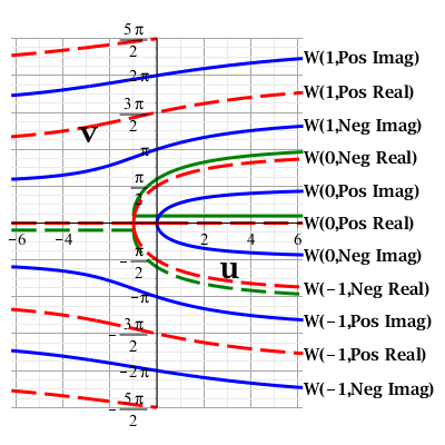
Figure 5: Branch 0 and -1 Real Lambert Lines. The real Lambert lines for branch 0 (for all real values of $z=x$) have been overlaid on the standard $w$-plane Lambert lines diagram, with the real Lambert lines for branch 0 drawn as a solid green curve, shifted up by $0.3$ to enable the green curve to be distinguished from the $v=0$ abscissa of the $w$-plane. The real Lambert line for branch -1 (for real values of $z=x<0$) have been overlaid on the standard $w$-plane Lambert lines diagram, with the real Lambert line for branch -1 drawn as a dashed green curve, shifted down by $0.3$ to enable the green curve to be distinguished from the abscissa of the $w$-plane.
——————————————————————————————

Branch 0: We have used a solid green line for branch 0, and added $0.3$ to the value of $v$, so that we are graphing

$$w = u+\mathbf{i}v+\mathbf{i}[\text{offset}]$$ (13)

$$= W_{0}(z)+0.3\mathbf{i}$$ (14)

for real $z=x$. This displays the $w$-plane images of both of the real axial rays of the $z$-plane. When $-1/e\leq x$, the branch 0 real Lambert line (solid green line) is horizontal, shifted 0.3 above the abscissa, and that portion of the Lambert line has $u\geq-1$. When $x<-1/e$, the $w$ values are complex, not real, and the branch 0 real Lambert line (solid green curve) goes up and to the right, starting from the point $(-1,0)$ (and shifted up by 0.3).

Branch -1: We have used a dashed green line for branch -1, and subtracted $0.3$ from the value of $v$, so that we are graphing

$$w = u+\mathbf{i}v-\mathbf{i}[\text{offset}]$$ (15)

$$= W_{-1}(z)-0.3\mathbf{i}$$ (16)

for real $z=x$ for which $x<0$. This displays only $w$-plane image of the negative real axial ray of the $z$-plane. When $-1/e\leq x<0$, the branch -1 real Lambert line for negative $x$ (dashed green line) is horizontal, shifted 0.3 below the abscissa, and that portion of the Lambert line has $u<-1$. When $x<-1/e$, the $w$ values are complex, not real, and the branch -1 real Lambert line for negative $x$ (dashed green curve) goes down and to the right, starting from the point $(-1,0)$ (and shifted down by 0.3).

Without the offsets, the dashed green curves would be exactly the dashed red curves, for the branch 0 real Lambert lines, and for the branch -1 real Lambert line for $x<0$.

2.2.2 How to Draw the Lambert Lines

It is perhaps worthwhile describing how the Lambert line curves can be produced using a standard symbolic mathematics software package. The curves in this document were drawn with Maple, but other software with a Lambert $W$ function implementation will be similar.

The technique is to draw a Lambert $W$ line as a parametric curve, with parameter $t$, for instance. Assume a branch number $k$. Assume an axial ray direction in the $z$-plane, denoted by $z_{0}$ equal to one of the four directions from the origin: $+1,\mathbf{+i},-1,-\mathbf{i}$. Then let the parameter $t$ vary between min and max limits, either linearly or logarithmically as suits the graphical requirements, and evaluate $w=W_{k}(tz_{0})$. This variable $w$ is a complex number. Define $u,v$ as the real and imaginary parts of $w$, and graph the parametric curve $(u(t),v(t))$ for $t=t_{min}...t_{max}$.

One further caveat: when $z\approx-1$, the value of $w$ can change rapidly. The real Lambert lines for branches 0 and -1 have a sharp corner at $z=-1$. Hence special care is needed near that point in the parametrization. It is simplest to draw those Lambert lines (branches 0 and -1, real Lambert lines near $z=-1$) as two distinct parametric curves, one for $z\leq-1$ and the other for $-1\leq z<0$, as each of those curve segments is a smooth curve.

2.2.3 Symmetry in the $w$-Plane

Because the values of $v\cot(v)$ and $v\tan(v)$ are unchanged if $v$ is replaced by $-v$, the Lambert lines (figure 1) are symmetric above and below the horizontal axis. Note however that the Lambert lines are not symmetric about the vertical axis.

It is sufficient, in many geometric explorations, to consider only the upper half of the $w$-plane. The exception is when there are ancillary equations in the problem which are not themselves symmetric in $v$. However, for an understanding of a system, it can nonetheless be convenient to show all four quadrants of the relevant curves in the $w$-plane and the corresponding curves in the $z$-plane. That leads to the two-planes method, which we will discuss in the next subsection.

2.3   What is the Two-Planes Method?

The two-planes method involves considering and comparing the solution curves for a problem, using both the $w$-plane and the $z$-plane. Recall that the mapping from the $w$-plane to the $z$-plane is $z=F(w)=w\,e^{w}$, and the mapping from the $z$-plane to the $w$-plane is the multi-branch Lambert $W$ function.

2.3.1 Illustration: FSW with Strength $R=5$

We illustrate with a 1-dimensional quantum FSW of strength $R$. Here $R$ is a dimensionless parameter, determined by the depth and width of the FSW. We will discuss the details of the factors which form the strength $R$, in the next section 3 of this paper.

Suppose that $R=5$. We wish to represent the simultaneous solutions of equations (1) and (2) in order to identify even bound states of the FSW. Draw a circle of radius $R=5$ about the origin, in the $w$-plane. This is shown in figure 6. The blue imaginary Lambert lines are the solutions of $u=v\tan(v)$, so the intersections of those Lambert lines with the $R=5$ circle identify the even bound state solutions of the FSW problem. We see, from figure 6, that there are two even bound states of the FSW in the first quadrant (where $u>0$ and $v>0$) and one bound state “solution” in the second quadrant (where $u<0$ and $v>0$).

Figure 6: Lambert Lines and Strength R=5 Circle. This figure shows the Lambert lines in the $w$-plane, with an FSW circle of strength $R=5.0$ superimposed. Dots have been placed to indicate where the strength circle intersects a Lambert line. The intersections of imaginary Lambert lines (blue solid curves) with the strength circle are solutions of $u=v\tan(v)$ and $u^{2}+v^{2}=5^{2}$, and indicate even bound states of the FSW. The intersections of real Lambert lines (red dashed curves) with the strength circle are solutions of $u=-v\cot(v)$ and $u^{2}+v^{2}=5^{2}$, and indicate odd bound states of the FSW.
——————————————————————————————

Similarly, the odd bound states of the FSW are represented by the simultaneous solutions of equations (1) and (3). Those solutions are intersections of the $R=5$ circle with the red real Lambert lines, since those lines are the solutions of $u=-v\cot(v)$. We see, from figure 6, that there are two odd bound states of the FSW in the first quadrant (where $u>0$ and $v>0$) and one bound state “solution” in the second quadrant (where $u<0$ and $v>0$).

All those intersections, for even bound states and for odd bound states, are marked in figure 6 with dots. However, we omitted the $u=R,v=0$ intersection since that is not a physically meaningful solution for an FSW.

2.3.2 Symmetry, Asymmetry, and $u<0$

Notice there is a symmetry among the solutions. Solutions for $v>0$ are paired with solutions for $v<0$. However, there is also an asymmetry: Equation (1) combined with one of either equation (2) (for even states) or equation (3) (for odd states) has solutions for $u<0$ which are not in the first quadrant of figure 6.

Are solutions for $u<0$ physically meaningful for an FSW model? They are certainly mathematically meaningful, as solutions of a pair of simultaneous equations which appear in a mathematical model of a physical system. The answer to that question, whether solutions with $u<0$ are physically meaningful, depends upon the specific structure of the physical system which has been described by a mathematical FSW-like model. For the present, we will continue to include the solutions with $u<0$ in our explorations.

2.3.3 Solutions in the $z$-Plane

Now, let’s ask what the corresponding solutions diagram looks like in the $z$-plane. The Lambert lines map into the axes of the $z$-plane, with the even bound states (on blue imaginary Lambert lines) going to the positive and negative imaginary axes, and with the odd bound states (on red real Lambert lines) going to the positive and negative real axes.

The circle $u^{2}+v^{2}=R^{2}$, which is a continuous closed curve in the $w$-plane, will go to a continuous closed curve in the $z$-plane, with multiple loops around the origin. See figure 7. There are large scale changes in the $z$-plane curve, because of the $\exp(u)$ factor seen in equation (2.2). Therefore the $z$-plane image of the strength circle for $R=5$ has been drawn in full in figure 7a, and at various zoomed-in magnifications in figures 7b, 7c and 7d.

(a) Complete Curve

(b) Magnified 16x

(c) Magnified 160x

(d) Magnified 1600x

Figure 7: $z$-Plane Image of Strength R=5 Circle. This figure shows the $z$-plane image of an FSW circle of strength $R=5.0$, at various magnifications in order to exhibit the detailed structure of the curve near the origin. The image curve is closed, just as the strength circle in the $w$-plane is a closed curve. The Lambert lines of the $w$-plane correspond to the axial rays of the $z$-plane. Hence, wherever the strength circle image crosses the imaginary axis ($x=0$) in the $z$-plane, there is an FSW even bound state indicated by a blue dot, and wherever the image crosses the real axis ($y=0$) there is an FSW odd bound state, indicated by a red dot.
——————————————————————————————

It is easy to draw that curve in the $z$-plane. Write $w=R\exp(\mathbf{i}\theta)$, where the angle $\theta$ goes from $0$ to $2\pi$, and walk around the $|w|=R$ circle in the $w$-plane, plotting $z=we^{w}$ in the $z$-plane. As can be seen in the various magnified views in figure 7, the blue dots, which indicate odd bound states of the FSW, all lie upon the imaginary axis ($x=0$), and the red dots, which indicate even bound states of the FSW, all lie upon the real axis ($y=0$). No dot was drawn at the point $(R,0)$ in the $z$-plane, because that is not a physically feasible state of the FSW.

The two-planes method provides two ways of viewing the properties of an FSW-like system. In the $w$-plane, the Lambert lines, which represent the algebraic relationships given by equations (2) and (3), are complicated curves, requiring one to be able to calculate Lambert $W$ function values, or at least to be able to calculate values of the tangent function. But in the $z$-plane, the Lambert lines are simply the imaginary and real axial rays, and can be drawn with a straightedge. On the other hand, the equation (1) which represents the strength of an FSW, is just a circle about the origin in the $w$-plane, and can be drawn with a compass. But in the $z$-plane, one has to draw the image of that strength circle by calculating an exponential, and also has to deal with changes of scale in the diagram.

Thus the two-planes method provides one with a choice of representations to use for solving a physical problem. As is familiar from other mathematical physics problems, the choice of a convenient coordinate system or representation of the physical system can make a problem either fairly easy to solve or uncomfortably difficult.

To assist in keeping track of the properties of the two types (imaginary and real) of Lambert lines, the colours and line styles used for those curves, and the two types of FSW bound states (even and odd) which those lines correspond to, we have appended Table 1 which records all that information on a single page.

3   3-D Representation of Sensitivity of Solutions

In this section, we wish to explore some techniques which are relevant to determining special solutions of a physical system. For example, a tangency which may suggest desirable parameters for a physical system used as a sensor, or alternatively may suggest an operating context in which a physical system may be so sensitive to parameter changes that it is prone to failure. We also wish to describe a method of introducing a third dimension into the $w$-plane and $z$-plane representations of the system, in order to visualize situations in which the behaviour of the system can change when a parameter is altered.

We will use a finite square well as our illustrative system. In this illustration, we will ignore the question of whether solutions with $u<0$ are physically meaningful. We are allowing the FSW to be a proxy for an FSW-like system, in which we are solving for intersections between a strength circle of radius $R$, and some Lambert lines.

What happens if the strength of the FSW changes? That may happen because the depth of the well changes, or because the width of the well changes. Those terms, depth and width, have a meaning appropriate to the particular physical system which is being modelled via an FSW. The depth, for instance, may be related to a bias voltage applied to a sensor. Since the FSW discussed here as an illustration is merely a proxy for other FSW-like systems, one can think of any other parameter, not necessarily strength of an FSW, which is an adjustment for the system, either at design or during operation.

3.1   Strength Formula for a Finite Square Well

Consider a 1-dimensional quantum finite square well. In a standard representation, found in quantum mechanics books, the FSW is described in terms of a width $L$ (a length) and a potential depth $V_{0}$ (an energy). For instance, an FSW might be stated to have a potential function $V(x)$ which is a fixed negative energy level, $V(x)=-V_{0}$ for $x$ satisfying $-L<x<L$. Outside the well, the potential function $V(x)=0$.

We call $L$ the half-width of the well, and $V_{0}$ (positive) the depth of the well. The energy $E$ of a bound state will be negative, and will satisfy $-V_{0}<E<0$. There are only a finite number of possible bound state energies for the FSW which will produce a stationary wave function which satisfies the Schrödinger equation.

We will not go through the details of finding the solutions here. Here, we simply wish to exhibit the formulas which determine the FSW strength $R$, and to indicate how the $u$ and $v$ values are determined once the bound state energy is known.

The relevant formulas are

$$R = \frac{L}{\hbar}\,\sqrt{2mV_{0}}$$ (17)

$$u = \frac{L}{\hbar}\,\sqrt{2m|E|}$$ (18)

$$v = \frac{L}{\hbar}\,\sqrt{2m(V_{0}-|E|)}$$ (19)

Here $m$ is the effective mass of the bound particle. Recall that $V_{0}$ is positive, that the bottom of the potential well is at $V(x)=-V_{0}$, and that the bound state energy $E$ is a negative value between 0 and $-V_{0}$. The symbol $\hbar$ is of course the reduced Planck-Einstein-Bose (PEB) constant. The positive signs assigned to $u$ and $v$ by the above formulas are conventional, and we are at liberty, depending upon the specifics of the system described via an FSW, to take the negative signs for the square roots. The FSW analytical work which leads to those formulas simply requires that $u,v$ satisfy

$$u^{2} = \frac{2m|E|L^{2}}{\hbar^{2}}$$ (20)

$$v^{2} = \frac{2m(V_{0}-|E|)L^{2}}{\hbar^{2}}$$ (21)

and also requires that $u,v$ be related by either $u=v\tan(v)$ or $u=-v\cot(v)$. That $R$ satisfies equation $u^{2}+v^{2}=R^{2}$ follows by adding together the two equations (20) and (21). All three of the quantities $u,v,R$ are dimensionless.

If $v=0$, then $E=-V_{0}$, which means, in a quantum FSW, that the bound state energy would lie exactly at the bottom of the well. That is unphysical, since such an energy would violate the uncertainty principle of quantum theory. For that reason, $v=0$ is excluded from the set of allowable solutions which we discuss here. However, there may be systems, classical perhaps, for which the mathematical solution $v=0$ might make physical sense. Here, for simplicity, and because the solutions with $v=0$ are not as interesting, we will assume that $v\neq 0$.

If $u=0$, then $E=0$, which means that the state with energy $E$ is not actually a bound state. The FSW potential outside the well is assumed to be zero, and a particle with energy $E$ would be uncertainly free, or uncertainly bound. That is a different situation than the system states which we are contemplating here, but suggests some physically interesting opportunities. For instance, scattering or resonance/delay of a free particle with low positive energy which passes over a potential well.

3.2   Tangency of Lambert Line and Strength Circle

We wish to explore the possibility that neither of $u,v$ is zero, and that the strength of the FSW is one of the special values which makes the strength circle tangent to a Lambert line. It is the hypothesis of this paper that such tangencies may be useful for designing sensors which utilize physical systems which are FSW-like. That is, these systems may be ones which have equations similar to equations (1) to (3) to be solved, and for which $u<0$ cases are meaningful in the model of the system. Our objective in this paper is to describe ways of working with such systems, using Lambert lines techniques.

With $R=5$, we observed in figure 6 that there are six bound states in the upper two quadrants ($V>0$) of the $w$-plane. Let’s draw some more strength circles. See figure 8, where the strength $R=5$ circle is represented by a solid curve. With strength $R=4.2$, represented by a dashed circle in the same figure, there are only four bound states in the upper half-plane. At strength $R$ slightly more than $R=4.6$, for example at $R=4.6034$ represented by a dotted circle, the circle has become tangent to the blue Lambert line and there are an uncertain number of bound states in the upper half-plane: maybe four bound states, or maybe six bound states, or maybe (on average) five bound states.

Figure 8: Lambert Lines and Three FSW Strengths. This figure shows the Lambert lines in the $w$-plane, with FSW strength circles of three different strengths superimposed. The solid circle is strength $R=5.0$, which was previously shown in figure 6. It intersects a Lambert line six times in the upper half-plane ($v>0$). The dashed circle is strength $R=4.2$ and it intersects a Lambert line only four times in the upper half-plane, so there are fewer bound states for the FSW. The dotted circle is strength $R=4.6034$ and it intersects a Lambert line 4 to 6 times. (The number of intersections is uncertain.) Two of those intersections, at $u=-1$ and $v\approx 4.4934$ coincide, where the strength circle is tangent to a Lambert line. An FSW with strength 4.6034 may be a candidate for design of a sensor.
——————————————————————————————

The strength $R=4.6034$ for the FSW thus represents a possible sensitivity, which is a guideline for the design of a sensor or an inherently unstable system. Two of the odd bound states are at almost the same phase angle. However, the phase angle can change by a few percent while the radius of the strength circle changes by only a small fraction of a percent. That is the sensitivity in the system. A slight change in the physical properties of the system being modelled via an FSW, perhaps due to flexure, or incoming energy, or a change in a bias voltage, may produce a change in the behaviour of the system. For instance, there may be an increase in the system’s specific heat, or a release of energy which has been pumped into a system which is at a quasi-stable equilibrium.

One can see that the energy level associated with a point of tangency is not the same as the energy level at which the FSW strength circle intersects the positive $v$-axis. Let $(u_{1},v_{1})$ denote the point of tangency when $R\approx 4.6034$. Then $u=-1$, and $v$ can be calculated from equation (1) to be $v\approx 4.4935$.

If one were designing a sensor with attention focused only on the system’s behaviour in the first quadrant of the $w$-plane, where $u>0$ and $v>0$, then one might decide to set the system’s strength to $R=3\pi/2$ or approximately 4.7124. That is about 2.3 percent more than the value of $R$ which corresponds to greatest sensitivity, if the system is one for which values $u<0$ have a physical meaning.

3.3   How to Find Points of Tangency

We wish to describe how to find $w$-plane points where the strength circle of an FSW is tangent to a Lambert line.

Fact 1: Tangency requires $u<0$.

The first observation is that tangencies arise only in quadrant 2 or 3 of the $w$-plane, when $u<0$. That may be seen geometrically. We can restrict our verification to the upper half-plane, where $v>0$, because the lower half-plane is a mirror image of the upper half-plane. Moreover, we can exclude the particular case of tangency to the real Lambert lines which pass through $(-1,0)$, because $v=0$ there (and because there is a sharp corner in the Lambert line curves at that point).

Each of the other Lambert lines in the upper half-plane is an increasing function. To see this, note that $u=v\tan(v)$ increases as $v$ increases within a horizontal band of values of $v$ which lies between two positive odd integer multiples of $\pi/2$ (see figure 3) so those Lambert lines go from the lower left asymptote of the band to the upper right asymptote of the same band. And similarly, $u=-v\cot(v)$ also increases within its band of asymptotes, from one even positive integer multiple of $\pi/2$ to the next, from lower left in the band to upper right.

Imagine a particular point $(u_{1},v_{1})$ on an upper half-plane Lambert line. A perpendicular from that point must descend down to the right, and hence intersect the $v=0$ axis at a point $(u_{2},0)$ for which $u_{2}>u_{1}$. For the Lambert line to be tangent to a circle about the origin, that perpendicular must pass though the origin, so we require $u_{2}=0$ for tangency. Hence $u_{1}<0$, which means that the Lambert line’s point of tangency must lie in quadrant 2.

Fact 2: If $(-1,v)$ lies on a Lambert line, then a strength circle of radius $R=\sqrt{1+v^{2}}$ will be tangent to that Lambert line.

Suppose that ($u_{1},v_{1})$ lies on a Lambert line, and $u_{1}=-1$ and $v_{1}>0$. We wish to show that the straight line from $(-1,v_{1})$ to the origin will be perpendicular to that Lambert line. The slope of a Lambert line is $dv/du$, and the slope of a radius of a circle from the origin is $v/u$. To have the Lambert line be perpendicular to the radius, the product of those two slopes must be -1. That is, we wish to verify that

$$\frac{dv}{du}\cdot\frac{v}{u} = -1,$$ (22)

or equivalently,

$$\frac{du}{dv}\cdot\frac{u}{v} = -1,$$ (23)

at the point $(-1,v_{1})$.

As before, we proceed by cases.

Case 1: Suppose that the Lambert line in question is an imaginary Lambert line, so that $u=v\tan(v)$ is the equation of the Lambert line. Multiply each side of $u=v\tan(v)$ by $\cos(v)$ to obtain $u\cos(v)=v\sin(v)$. Differentiate both sides, to obtain

$$du\,\cos(v)-dv\,u\sin(v) = dv\,\sin(v)+dv\,v\cos(v)$$ (24)

Transposing and simplifying, we get

$$du\,\cos(v) = dv\,[(u+1)\sin(v)+v\cos(v)]$$ (25)

$$\frac{du}{dv} = \frac{(u+1)\sin(v)+v\cos(v)}{\cos(v)}$$ (26)

$$\frac{du}{dv} = (u+1)\tan(v)+v$$ (27)

Since $u=v\tan(v)$, this last equation becomes

$$\frac{du}{dv} = \frac{u(u+1)}{v}+v$$ (28)

Multiplying by $u/v$ gives

$$\frac{du}{dv}\cdot\frac{u}{v} = \frac{u^{2}(u+1)}{v^{2}}+u$$ (29)

Now suppose that $u=-1$. Then the first term in the last expression disappears, and the second term is $-1$, which means that the radius of the strength circle is tangent to the Lambert line. That completes the proof of case 1.

Case 2: Suppose that the Lambert line in question is a real Lambert line, so that $u=-v\cot(v)$ is the equation of the Lambert line. Quite similar to case 1. One ends up with equations (28) and (29) as in case 1, and then taking $u=-1$ completes the proof.

Figure 9 shows the FSW bound state solutions for the first four critical strengths: $R=2.9717,4.6034,6.2024,7.7898$.

(a) Tangency at $(-1,2.7984)$

(b) Tangency at $(-1,4.4934)$

(c) Tangency at $(-1,6.1213)$

(d) Tangency at $(-1,7.7253)$

Figure 9: Tangencies of the FSW Strength Circle. This figure shows the tangency of an FSW strength circle to a Lambert line, for four different values of the strength $R$. Each point of tangency lies upon the vertical line $u=-1$.
——————————————————————————————

In order to find the critical strengths $R$, we are essentially moving up along the vertical line $u=-1$ in the $w$-plane. A very interesting diagram results if we map the line $u=-1,v>0$ to the $z$-plane. It is a spiral (see figure 10), which intersects one of the four axial rays in the $z$-plane at $z$-values which can be used to determine the $R$-values which are the critical strengths. Given a $z$-value, we can calculate $w=W_{k}(z)$ for the appropriate branch number. The $v$ coordinate of the point of tangency in the $w$-plane is the imaginary component of $w$. The critical strength $R$ can then be calculated from $v$. Moving back to the $z$-plane, we can determine the magnitude of the corresponding $z$-value, via

$$|z| = |w|\exp(u)=\frac{|w|}{e}=\frac{R}{e}.$$ (30)

That, of course, gives a formula which can be used directly, $R=e\,|z|$, for determining the critical radius from a knowledge of the $z$ values for which the $z$-plane image of the $u=-1$ line from the $w$ plane intersects one of the axial rays in the $z$-plane. There is no need to determine the branch number of the Lambert $W$ function in order to find the critical $R$ values. The consecutive critical $R$-values on the vertical line $u=-1,v>0$ in the $w$-plane, are spaced about $\pi/2$ apart. The magnitudes of their $z$-plane images are spaced about $\pi/2e\approx 0.5779$ apart in the $z$-plane. Those $z$-values are distributed among the four axial rays from the origin, so along each axial ray the magnitudes of the $z$ values are spaced about $2\pi/e\approx 2.3115$ apart.

Figure 10 shows the $z$-plane image of the $w$-line $(-1,v)$ for $v>0$. Dots have been placed on the axial rays for the first 19 critical strengths $R$.

Figure 10: $z$-Plane Image of $u=-1,v>0$ Line. This figure shows the image, in the $z$-plane, of the vertical line $u=-1,v>0$ in the $w$-plane. Dots have been placed where the curve crosses one of the axial rays. These correspond to intersections of the vertical line $u=-1$ with Lambert lines in the upper half of the $w$-plane, which are points where an FSW strength circle of a critical radius will be tangent to a Lambert line.
——————————————————————————————

3.4   3-Dimensional Representation of Tangency

The original impetus for preparing this document was a desire to extend the two-planes method to a 3-dimensional representation, in order to use geometric methods to visualize systems which are FSW-like, that is, which include equations such as (2) and (3), and which also include a parameter such as the strength $R$ of an FSW, or the refractive index $n$ of a dielectric in a waveguide.

Conceptually, one can think of the four FSW solutions shown in figure 9 as slices of a 3-dimensional space, with different values of the FSW strength $R$. Thus $R$ is the third dimension in a visualization. The curved Lambert lines become curved sheets, call the Lambert sheets for convenience. The surface which represents the strength circles $u^{2}+y^{2}=R^{2}$ in three dimensions is a cone, with its point at the origin $(u,v,R)=(0,0,0)$. Simultaneous solutions of equation (1) and one of equations (2) or (3), are the curves where the FSW strengths cone intersects the Lambert sheets.

Our first attempts to demonstrate this geometry, by drawing the two types of surfaces and highlighting their intersections, were not satisfactory. The diagrams have too much clutter to allow clear reasoning about the situation.

Instead, we have chosen to show only the lines of intersection of the surfaces. One must imagine the Lambert sheets and the FSW strengths cone whose intersections produce those intersection lines.

Figure 11 has some views of the FSW lines of intersection. Each figure 11a to 11d shows a different view of the 3-D lines of intersection.

(a) Projected along $v$ axis. Shows that critical points occur at $u=-1$.

(b) Projected along $u$ axis. Shows relationship of $v$ and $R$ at critical points.

(c) Projected along $R$ axis. Shows relationship of $u$ and $v$ at critical points.

(d) Tipped to show all 3 axes. Demonstrates Lambert lines as 3-D curves.

Figure 11: Three-Dimensional View of Intersections of Lambert Line Sheets and the Cone of FSW Strength Circles. All points represent a bound state of a finite square well of strength $R$. Critical points are tangencies which possibly represent good sensor configurations.
——————————————————————————————

In figure 11a, we see a projection along the $v$ axis, so that this figure is essentially a graph of $R$ vs $u$. There are four curves of intersection shown, because four Lambert sheets have been included in the diagram. The $R$ value along the vertical axis of the diagram has a maximum of 8.7, and the $v$ values are given by $v=\sqrt{R^{2}-1}$, which thus has a maximum value of about 8.65, less than $3\pi$, so there are only four Lambert sheets of interest. (We have omitted the Lambert sheets which do not produce a tangency with the $R$-cone.) The number of intersection lines would be more if the diagram had been drawn to include a larger maximum value for $R$. Faint dotted lines have been included to pass through the $R$-minima of each of the curves shown, with tick marks along the vertical $R$-axis to illustrate that those minima correspond to the critical $R$-values exhibited in figure 9. One can also see, in figure 11a, that all the critical $R$-values correspond to $u=-1$.

In figure 11b, we see a projection along the $u$ axis. There are again four curves of intersection shown. Faint dotted lines pass through the critical points. The critical FSW strengths $R$ are marked on the vertical axis, and the corresponding values of $v$ are marked on the horizontal axis.

In figure 11c, we see a projection along the $R$ axis. This shows the relationship of $u$ and $v$, which of course is the same curves that are shown in a 2-dim Lambert lines diagram. The difference is that the 3-dim curve, if rotated to show the $R$ axis, would display $(u,v,R)$ points where $R=\sqrt{u^{2}+v^{2}}$.

In figure 11d, the 3-dim diagram has been rotated to show all three axes. Working with this, and similar, diagrams in a 3-dim graphics software package can be an aid to understanding the bound states of an FSW.

It is our belief that 3-dim methods such as have been used in this section for a finite square well, can also provide insight into the properties of FSW-like systems. In future reports, we wish to extend the techniques used above, to other FSW-like systems.

4   Discussion and Conclusions

In this paper, we have shown that the geometric display of the bound state energies of a 1-dimensional finite quantum square well (FSW) provides a convenient visualization of FSW strengths which can be useful for designing sensors. As well, we have exhibited a 3-dimensional visualization of the bound state solutions, and of the critical strengths of an FSW.

Type of
Lambert Line	Imaginary	Real
Equation in $w$-plane
where $w=u+\mathrm{i}v$	$u=v\,\tan(v)$	$u=-v\,\cot(v)$
Intersects ordinate
at $v=\pi/2$ times an	EVEN integer	ODD integer
Asymptotes cross ordinate
at $v=\pi/2$ times an	ODD integer	EVEN integer
Shown in figures as	BLUE SOLID	RED DASHED
Axial ray in $z$-plane	$x$ is equal to 0	$x>0$ or $x<0$
where $z=x+\mathrm{i}y$	$y<0$ or $y>0$	$y$ is equal to 0
FSW bound state
wavefunctions are	EVEN functions	ODD functions

Table 1: Lambert Line Properties and Notation

References

- [1] Ken Roberts and S. R. Valluri, “Solution of the quantum finite square well problem using the Lambert W function”, Arxiv 1403.6685v1, 2014.
-
[2]
Ken Roberts and S. R. Valluri,
“Tutorial: The quantum finite square well
and the Lambert W function”,
Canadian Journal of Physics,
vol 95 (2017), pp 105-110.
doi:10.1139/cjp-2016-0602.
A preprint of this tutorial is available online at
https://ir.lib.uwo.ca/physicspub/32/ - [3] David Bohm, Quantum Theory, Prentice-Hall, 1951. Dover reprint, 1989.
- [4] B. H. Bransden and C. J. Joachain, Introduction to Quantum Mechanics, Longman, 1989.
- [5] Paul C. W. Davies and David S. Betts, Quantum Mechanics, 2nd edition, Chapman and Hall, 1994.
- [6] David J. Griffiths, Introduction to Quantum Mechanics, 2nd edition, Pearson, 2005.
- [7] R. M. Corless, G. H. Gonnet, D. E. G. Hare, D. J. Jeffrey and D.E. Knuth, “The Lambert W Function”, Advances in Computational Mathematics, vol 5 (1996), pp 329-359.
-
[8]
S. R. Valluri, D. J. Jeffrey and R. M. Corless,
“Some applications of the Lambert W function to physics”,
Canadian Journal of Physics,
vol 78 (2000), no 9, pp 823-831.
doi:10.1139/p00-065.
A preprint of this article is available online at
https://www.uwo.ca/apmaths/faculty/jeffrey/pdfs/physics.pdf -
[9]
Frank W. J. Olver, Daniel W. Lozier,
Ronald F. Boisvert and Charles W. Clark (eds),
NIST Handbook of Mathematical Functions,
Cambridge, 2010.
This handbook is available online at
https://dlmf.nist.gov - [10] István Mező, The Lambert W Function: Its Generalizations and Applications, CRC Press, 2022.