Design and Evaluation of a Generic Visual SLAM Framework for Multi-Camera Systems

Abstract

Multi-camera systems have been shown to improve the accuracy and robustness of SLAM estimates, yet state-of-the-art SLAM systems predominantly support monocular or stereo setups. This paper presents a generic sparse visual SLAM framework capable of running on any number of cameras and in any arrangement. Our SLAM system uses the generalized camera model, which allows us to represent an arbitrary multi-camera system as a single imaging device. Additionally, it takes advantage of the overlapping fields of view (FoV) by extracting cross-matched features across cameras in the rig. This limits the linear rise in the number of features with the number of cameras and keeps the computational load in check while enabling an accurate representation of the scene. We evaluate our method in terms of accuracy, robustness, and run time on indoor and outdoor datasets that include challenging real-world scenarios such as narrow corridors, featureless spaces, and dynamic objects. We show that our system can adapt to different camera configurations and allows real-time execution for typical robotic applications. Finally, we benchmark the impact of the critical design parameters - the number of cameras and the overlap between their FoV that define the camera configuration for SLAM. All our software and datasets are freely available for further research.

I Introduction

Simultaneous Localization and Mapping (SLAM) is a fundamental task required for the autonomous navigation of mobile robots. Visual SLAM (VSLAM) is one of the more favored approaches as cameras are inexpensive, easily deployable, low-power sensors which provide rich information about the world in which the robot operates. Most of the VSLAM pipelines[1][2][3] use monocular cameras prone to a single point of failure due to degenerate motion, illumination changes, featureless surfaces and, dynamic objects. They are further limited by a small field of view and inconsistencies associated with scale. Additional sensors such as Inertial Measurement Units (IMUs) or LIDAR can be used to improve performance in these scenarios. The former can cause large accumulated errors in visual tracking failure due to noisy sensor inputs, and the latter can be expensive in terms of both cost and weight. On the other hand, multi-camera systems strike a good balance between data quality and cost. They can capture more visual information and offer the advantage of redundancy, which helps improve robustness and better constraints for localization and mapping. As a result, multi-camera sensing has attracted much research interest in recent times leading to novel SLAM solutions, datasets, and implementations on robotic platforms.

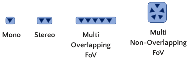
(a)

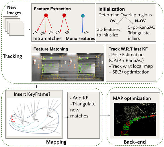
(b)

Figure 1: (a) Illustration of various overlapping(OV) and non-overlapping(N-OV) camera configurations evaluated in this work. (b) Block diagram of the generic visual SLAM framework showing its sub-modules. Feature extraction computes two types of features–multi-view intra-matches and regular mono features. Note the changes,made to initialization, tracking and keyframe representation to adapt to a general multi-camera system.

Many earlier works on multi-camera SLAM are designed for a particular camera rig and do not exploit the camera arrangement to the fullest. In this paper, we look at the much more general case of multiple overlapping and non-overlapping cameras. We build upon the ideas presented in [4] but differ in terms of modeling the camera system making it extensible to multiple overlapping views beyond stereo pairs. We use a generalized camera model to represent the multi-camera system as a collection of unconstrained rays without making any assumptions about a particular geometry. Another challenge with multiple cameras is to effectively and efficiently utilize the increased amount of information provided by the sensors. We compute the overlapping regions among the component cameras in the rig and extract 3D features via cross-matching. This leverages the camera configuration to fuse multi-view data, avoids duplicating features, and keeps the computational cost in check.

Realizing practical mobile robotics applications requires designing sensor systems along with algorithmic development. The choice of cameras and the system configuration of the sensing platform impacts the SLAM outcome. While there have been significant efforts towards developing SLAM algorithms for different sensors, there has been a lack of attention to the system design aspects of the sensing platform. To address this gap, we identify the number of cameras and the overlap between their FoVs as two key design parameters of the system configuration that impact the information gathered by the cameras and, thus, SLAM estimates. We evaluate the localization accuracy and robustness of our SLAM system on several real-world datasets collected using our custom-built multi-camera rig. The major contributions of this paper include

• An open source generic visual SLAM framework with a carefully designed front end and back end that works with arbitrary camera setups.

• A collection of six real-world indoor and outdoor datasets on which the developed SLAM system is evaluated. These datasets are complementary to existing datasets and were collected specifically to highlight problems with current VSLAM implementations.

• A systematic experimental evaluation of the SLAM framework in terms of tracking accuracy, robustness, and computational constraints.

• A detailed analysis of the effect of the camera configurations on SLAM for monocular, stereo, and multi-camera setups with and without overlapping FoVs.

II Related Work

There is a large body of literature on visual SLAM that focuses on monocular, stereo or RGBD cameras, and exploits their intrinsic and extrinsic properties. For instance stereo and RGBD cameras are used to obtain metric SLAM estimates[2][5][6] in contrast to the monocular SLAM[1] with bearing-only image data. Within the monocular SLAM realm, wide field-of-view (FoV) and omnidirectional cameras have been used for SLAM[7][8][9]. There are many state-of-the-art SLAM pipelines that work off the shelf in a plug-n-play fashion[3][10].

Multi-camera SLAM has gained attention recently due to its robustness and superior perception capabilities. One of the first multi-camera SLAM frameworks was discussed by Sola et al[11], where data from multiple independent monocular cameras is fused via filtering. Kaess et al[12] propose a probabilistic approach to iteratively solve data association and SLAM for a circular 8 camera rig. They show that allowing cameras to face different directions yields better constraints and helps with loop closures irrespective of robot orientation. MultiColSLAM [13] extends ORBSLAM to a rigidly coupled fish-eye multi-camera system by modeling the camera cluster as a generalized camera [14]. Zhang et al[15] present a SLAM system that also calibrates extrinsic parameters using wheel odometry. These works mainly target non-overlapping camera setups that provide maximal coverage of the surroundings and do not exploit the overlap between cameras. Other similar contributions include [16][17][18].

A few works employ stereo pairs to obtain 3D features via stereo matching between overlapping areas and recover metric scale. Heng et al[19] use four fish-eye cameras arranged as two stereo pairs facing forward and backward to give 360^∘ view. ROVO[20] uses the same camera configuration, but applies a hybrid projection model to minimize distortion and maximize feature matching. In [21], a multi-stereo pipeline is presented with a new 1-point RANSAC for joint outlier rejection. In [22] and its follow up work[23], show that multiple stereo pairs improve the feature space for tracking while driving at night from several real-world experiments. In[24], a linear front-facing camera array is used to perform Light Field based static background reconstruction to handle dynamic objects. Li et al [25], perform robust initialization and extrinsic calibration in multi-camera systems with limited view overlaps. Zhang et al[26] use submatrix feature selection to reduce compute and track features across stereo and mono cameras. However, these methods assume a priori knowledge about the camera configuration. Kuo et al[4], present an adaptive SLAM design to accommodate arbitrary camera systems. However, it is not clear if the system can handle overlapping configurations beyond stereo since the method focuses on finding stereo pairs and all the experiments were evaluated on stereo pairs only.

Studying the impact of camera system design will enable us to build robust multi-camera systems for mobile robots. Nevertheless, the research in this direction is still in the nascent stages. Zhang et al[27] discuss the impact of field-of-view of a monocular camera on visual odometry in urban environments. Kevin et al[28] benchmark commercially available monocular, stereo and RGB-D sensors by evaluating them on the OpenVSLAM framework. In [16], the authors evaluate MCPTAM on overlapping and non-overlapping camera clusters and show that overlapping cameras recover accurate scale and cause less drift. We add on to these efforts by evaluating the impact of the number of cameras and their extrinsic arrangement on SLAM.

(a)

(b)

Figure 2: Two sample multi-camera frames showing features extracted in the images from (a) front-facing cameras in overlapping (OV) setup and, (b) three cameras in non-overlapping (N-OV) setup for the same scene. The colored points are the multi-view features where closer points are red and farther points are blue. The white points are the mono features which do not have any 3D information. Notice that N-OV setup has only mono features, where as the OV setup has both multi-view and mono features distributed across overlapping and non-overlapping regions in the images.

III Problem Setup

The primary goal of our VSLAM formulation is to develop a unified framework independent of the camera system configuration, which is lightweight and runs in real time on mobile robots. The block diagram of the generic visual SLAM pipeline is shown in fig. 1.

Definitions: Let the number of cameras in the sensor rig be $N_{c}$, where $N_{c}>=1$. Each component camera $c_{p}$ is related to the body frame of the multi-camera rig by a rigid body transformation ${}^{B}T_{p}=\{{}^{B}R_{p},{}^{B}t_{p}\}$ obtained via extrinsic calibration parameters. The intrinsic parameters of the component cameras are denoted as $K_{p}$. Estimated keyframe poses are represented as $x_{n}\in SE(3)$, $n\in{1...N}$ and correspond to the rig body frame with respect to the world ${}^{w}T_{B}$. The landmarks are represented as $l_{m}\in R^{3}$ with $m\in{1...M}$. The visual measurements of the landmarks in the images are denoted as $z_{k}\in R^{2}$ with $k\in{1...K}$, the data association that relates each measurement $z_{k}$ with a keyframe, component camera, and a landmark is given by $(x_{n_{k}},c_{p_{k}},l_{m_{k}})$. We assume the body frame of the rig to align with one of the camera coordinate frames for simplicity.

Camera Configuration: An arbitrary camera configuration is the most generic definition, which encompasses all the ways a set of cameras can be rigidly arranged on a robotics platform. For example we can use monocular or stereo setups, or cameras lying on a circular ring with the possibility of overlapping or non-overlapping FoV. We distinguish different camera configurations based on- the number of cameras ($N_{c}$) and the FoV overlap among them, and benchmark their influence on SLAM. For this study, for the purposes of clarity, we have scoped our work solely on either overlapping (OV) or non-overlapping (N-OV) (shown in fig. 1a) scenarios even though the methodology is generally applicable to mixing both overlapping and non-overlapping camera rigs. Irrespective of the configuration, the multi-camera rig is considered as a single generalized camera that captures a collection of rays passing through multiple pinholes which will be detailed in section IV.

IV The Front-end

The front end of a SLAM system aims to estimate the pose of the robot and the landmarks observed at each time step. This section discusses the critical aspects of feature extraction and representation, initialization, tracking, and mapping modules that enable us to seamlessly work with arbitrary multi-camera systems.

IV-A Feature Extraction

We perform sparse feature tracking using two types of features - Multi-view features and Mono features. Depending on their placement, the cameras comprising the camera rig can have overlapping fields of view. We leverage the overlapping imagery to compute strong metric features. Instead of using the features extracted from component cameras independently, we associate overlapping image regions to group features that belong to a specific 3D point in the scene. This differs from most existing camera systems which do not utilize overlap among cameras except to compute stereo. Our multi-view features let us accurately represent the scene with fewer features and avoid creating redundant landmarks during SLAM.
Determining Overlap: This is the first step required to compute multi-view features efficiently. For each component camera $c_{i}$, we find the common image regions in the set of cameras $\mathcal{C}$ that share a common FoV with $c_{i}$. Starting with a camera pair ($c_{i},c_{j}$), we first divide the image of $c_{i}$ into a 2D grid. For each grid cell $g_{k}$, the epipolar line $e_{ij}^{k}$ corresponding to its center $g_{k}^{x},g_{k}^{y}$ is computed using extrinsic calibration between the camera pair as shown below.

$$F_{ij}=K_{j}[{}^{j}t_{i}]_{\times}{}^{j}R_{i}K_{i}^{-1}$$ (1)

$$e_{ij}^{k}=F_{ij}[g_{k}^{x},g_{k}^{y}]$$ (2)

Next, we determine the grid cells in the image of $c_{j}$ that the epipolar line passes through and save them as potential cells to find correspondences. If the line does not pass through the image plane, we know that the camera pair is non-overlapping. This computation is done just once during initialization in the beginning of and then used throughout the run while executing the SLAM framework.
Multi-view Features: These are essentially cross-matches between cameras. First, we extract multi-scale ORB features in all images and assign them to the 2D grid. This process is parallelized for speed. We then iteratively compute feature correspondences between each unique pair of cameras resulting in a total of $N_{c}\mathcal{C}_{2}$ combinations for $N_{c}$ cameras. For a camera pair ($c_{i},c_{j}$), instead of matching every feature in $c_{i}$ to every feature in $c_{j}$, we match features cell-wise based on the overlap to reduce computation. For a set of features, $\mathcal{F}1$, belonging to a cell in the image of $c_{i}$ we obtain the set of features $\mathcal{F}2$ lying in the cells corresponding to the potential matches obtained from the overlap determination step. We then perform brute-force matching between the sets $\mathcal{F}1$ and $\mathcal{F}2$. Each match is then passed through the epipolar constraint which checks if the corresponding feature in the second view is within a certain distance from the epipolar line. A set of matches $\mathcal{M}$ is created from the first pair of cameras. For the subsequent image pairs, if correspondence is found between two unmatched features, a new match is added to the set of matches $\mathcal{M}$. If a match is found for an already matched feature, the new feature is added to the existing match.

Each multi-view match represents a 3D feature in the scene. It consists of a bundle of rays given by a set of 2D keypoints, which are projections of the 3D feature in component cameras, the 3D coordinate obtained from triangulation, and a representative descriptor computed to facilitate feature matching for tracking. Note that the 3D point does not need to be observed in all the cameras. The observability depends on the overlap and scene structure.

Mono Features In the case of either a monocular camera or non-overlapping camera configurations, there are no multi-view matches. Even within overlapping camera configurations, there might be some non-overlapping regions depending on the structure of the 3D scene. We have mono features with a single 2D keypoint and its descriptor to represent the non-overlapping areas.

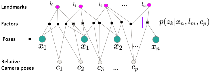
Figure 3: Factor graph of the multi-camera back-end. The poses $X_{i}$, landmarks $l_{j}$ and the relative camera poses $C_{p}$ are the variables to be optimized. The factors are shown as black square nodes and represent the constraints on the variables.

IV-B Initialization

This step creates the initial set of landmarks which are used to track subsequent frames. we perform initialization based on the underlying camera configuration. After extracting features, if the number of metric multi-view features is greater than a certain threshold, we utilize them as the initial map. Otherwise, we have to choose two initial frames and compute the relative pose between them. We use a generalized camera model which allows non-central projection suitable to represent multi-camera systems[14]. A key point expressed as a pixel, $u$, in the image of camera $c_{p}$, is represented as a Plucker line $L=[q\;\;q^{\prime}]$ which is a 6-vector made of line direction $q$ and moment $q^{\prime}$.

$$\hat{u}=K_{p}^{-1}u,\;\;q={}^{B}R_{p}\hat{u},\;\;q^{{}^{\prime}}={}^{B}t_{p}\times q$$ (3)

we determine correspondences between two frames and solve the generalized epipolar constraint to obtain relative pose

$$\begin{pmatrix}q_{2}\\ q_{2}^{{}^{\prime}}\end{pmatrix}^{T}\begin{pmatrix}E&R\\ R&0\end{pmatrix}\begin{pmatrix}q_{1}\\ q_{1}^{{}^{\prime}}\end{pmatrix}=0$$ (4)

where,$[q_{1}\;q_{1}^{{}^{\prime}}]$ and $[q_{2}\;q_{2}^{{}^{\prime}}]$ are the Plucker rays of matched features, $E=[t]_{\times}R$ is the essential matrix with $R$ and $t$ being the rotation and translation between the two generalized camera frames. In the case of a monocular camera, the Plucker ray corresponding to the keypoints is $[\hat{u}\;\;0]$ from eq(3). Thus the generalized epipolar constraint is naturally reduced to the classical epipolar constraint. We apply the 5-point algorithm for a monocular camera and the 17-point algorithm[29] for a multi-camera rig with RANSAC for relative pose estimation. We make sure that there is sufficient parallax between the two frames and triangulate the correspondences which act as our initial landmarks, and follow this with non-linear optimization to obtain our final landmark estimates

IV-C Tracking and Mapping

After initialization, every incoming frame is tracked with respect to the last keyframe. We compute inter-frame correspondences between the last keyframe and the current frame via bag-of-words matching. Since multi-view features contain more than one descriptor from different component cameras we use the median of descriptors for matching. If enough 3D-2D matches are found between the map points ${}^{w}P_{i}$ in the last keyframe and observations $z_{k}$ in the current frame we obtain the Plucker coordinates of $z_{k}$, $[q_{k}\;\;q_{k}^{{}^{\prime}}]$ using eq (3) and estimate the absolute pose of the current frame $[{}^{B}R_{w}\;\;{}^{B}t_{w}]$ using generalized PnP[30] by solving a set of constraints of the form

$$\lambda q_{i}+q_{i}\times q_{i}^{{}^{\prime}}={}^{B}R_{w}{}^{w}P_{i}+{}^{B}t_{w}$$ (5)

If the estimated pose indicates significant motion since the last keyframe we further localize the current frame with respect to the local map in a manner similar to ORBSLAM. We find the set of neighboring keyframes $\mathcal{K}$ shared by the initially tracked landmarks. We then compute new matches between the landmarks tracked in $\mathcal{K}$ and the current frame. This enables us to gain local map support and helps in finding stable landmarks in the presence of occluding dynamic objects. Finally, the current frame is inserted as a keyframe if the ratio of the tracked landmarks since the last keyframe is less than a certain threshold. When a new keyframe decision is made, the observations are added to the existing landmarks and the new inter-frame matches corresponding to the non-map points are triangulated to create new map points.

V The Back-end

The back end corresponds to the optimization framework that refines the initial estimates of keyframe poses $X$ and landmarks $L$ by maximizing the posterior probability on the variables given observations $Z=\{z_{k}\}_{k=1}^{K}$[31]. In a general multi-camera system an observation not only depends on the pose of the rig $X$ and the landmark $L$, but also on the component cameras $C$ it is seen in. The Maximum a Posteriori (MAP) problem is given by

$$X^{*},L^{*},C^{*} =\underset{X,L,C}{argmax}\;P(X,L,C\;|Z)$$

$$\propto\underset{X,L,C}{argmax}\;P(Z\;|X,L,C)\;P(X,L,C)$$

$$\propto\underset{X,L,C}{argmax}\;P(x_{0})\prod_{k=1}^{K}P(z_{k}|x_{n_{k}},l_{m_{k}},c_{p_{k}})$$ (6)

where $P(Z|X,L,C)$ is the likelihood of the observations which factorizes into a product of individual probabilities due to i.i.d assumption. $P(x_{0})$ is the prior probability over the initial robot pose. The factor graph representation in fig. 3 shows the individual probability constraints(factors) among variables. Assuming normally distributed zero-mean noise for the observations $z_{k}$ and modeling prior also as a gaussian eq(6) takes the least-squares minimization form

$$X^{*},L^{*},C^{*}\triangleq\underset{X,L,C}{argmin}\sum_{k=1}^{K}\|{h_{k}(x_{n_{k}},l_{m_{k}},c_{p_{k}})-z_{k}}\|^{2}_{\Sigma_{k}}$$

$$-log\;p(x_{0})$$ (7)

where the measurement function $h_{k}(x_{i_{k}},l_{j_{k}},c_{p_{k}})$ maps a landmark to a predicted observation $\hat{z_{k}}$ through a series of transformations. First, pose of the body $x_{n_{k}}={}^{w}T_{B}^{n}$ and the relative pose of the component camera $c_{p_{k}}={}^{B}T_{p_{k}}$ are used to get the pose of the camera in world frame via SE(3) composition ${}^{w}T_{c}={}^{w}T_{B}^{n}.{}^{B}T_{c}$. The 3D landmark $l_{m_{k}}=P^{w}$ is transformed from world frame into the camera coordinate frame $P^{c}=f(T_{c}^{w},P^{w})=(R_{c}^{w})^{T}(P^{w}-t_{c}^{w})$. Finally, $P^{c}$ is projected to 2D image coordinates using intrinsic matrix $\hat{z_{k}}=K_{c}P^{c}$ This formulation conveniently models multi-view features. It gives the back end the flexibility to work with different camera configurations and optimize the extrinsic calibration parameters of the component cameras $C$ along with estimating the trajectory and landmarks.

Datasets
Label	Location	Total Frames	Length (m)	Groundtruth	Attributes	Loop
ISEC_Lab1	indoor Lab	9130	152	optitrack	feature less areas , reflective surfaces	Yes
ISEC_Ground1	indoor lobby	4481	90	target based	reflective surfaces, minimal dynamic content, day light	Yes
ISEC_Ground2	indoor lobby	5408	90	target based	reflective surfaces, minimal dynamic content, night	Yes
ISEC_Ground3	indoor lobby	6001	120	target based	reflective surfaces,high dynamic content, day light	Yes
Falmouth	outdoor offroad	9156	2800	target based + gps	fast motion, outdoor, foliage, minimal dynamic content, large area	Yes
Curry_center	campus	28526	590	target based	Urban,outdoor,dynamiccontent,largearea	Yes

TABLE I: This table describes the attributes of the dataset used to evaluate the proposed SLAM framework. We collected six sequences with trajectory lengths ranging between 90 m - 2800 m in a wide variety of indoor and outdoor environments.

VI Experimental Setup

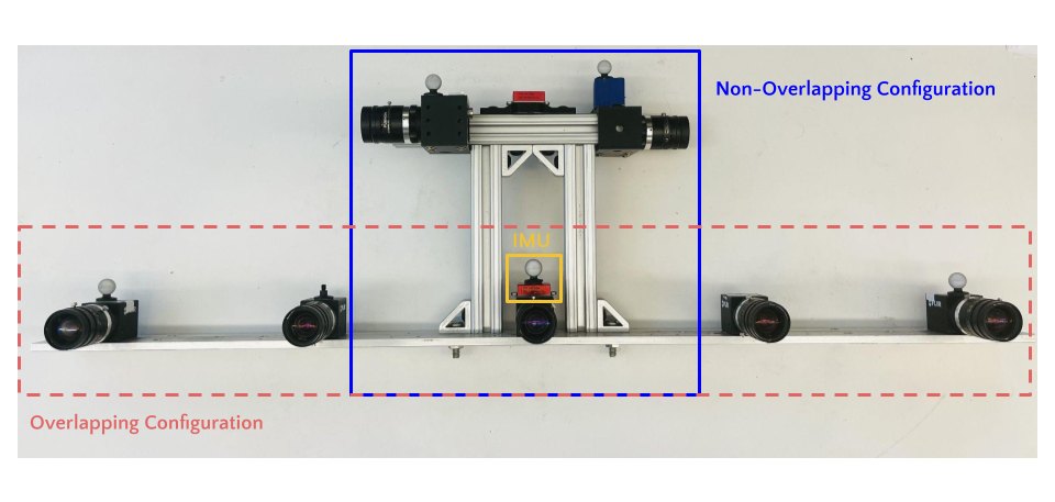
Figure 4: The custom-built multi-camera rig used to collect data for evaluating the SLAM pipeline. The figure shows overlapping and non-overlapping configurations, and the IMU that was mounted on the rig. The IMU is used to compute The baseline between two consecutive cameras is 165mm.

In this section, we describe the hardware setup, camera calibration, and collection of several indoor and outdoor datasets required to carry out the experimental evaluation.

VI-A Hardware Setup and Camera Calibration

We use a rigid multi-camera rig consisting of seven cameras with five cameras facing forward and two cameras facing sideways, and an inertial measurement unit (IMU) as shown in the figure fig. 4. The cameras are arranged to accommodate configurations with both overlapping(OV) and non-overlapping(N-OV) fields of views as shown in fig. 4. The front-facing cameras(red dashed box) are used to run experiments for mono, stereo, and overlapping multi-camera setup. The front-facing center camera and the side-facing cameras(blue box) are used as a non-overlapping multi-camera setup. We use FLIR BlackFly S 1.3 MP color cameras with a resolution of 720 x 540 and a FOV of 57^∘ and a Vectornav’s IMU running at 200 HZ. All the cameras are hardware triggered for synchronized capture at 20 fps.

We use Kalibr [32] to obtain the intrinsic and extrinsic parameters of the cameras with overlapping FOV using a calibration target. For non-overlapping cameras, target based calibration does not work as we need the cameras to observe a stationary target to solve for the relative transformation. Instead, we perform imu-camera calibration for each of the non-overlapping cameras and chain the inter-camera transformations together. This gives a good initial estimate of extrinsic camera parameters which is refined during optimization as described in section V.

	ISEC Lab1		ISEC Ground1 (non dynamic)		ISEC Ground2 (night)		Curry Center		Falmouth
Algorithm	ATE(m)	ATE(%)	ATE(m)	ATE(%)	ATE(m)	ATE(%)	ATE(m)	ATE(%)	ATE(m)	ATE(%)
2 cams	2.65	1.7	0.99	1.07	2.41	2.51	1.18	1.5	210.02	8.05
3 cams	1.23	0.8	0.350	0.38	2.38	2.47	0.482	0.63	48.744	1.87
4 cams	0.84	0.56	0.321	0.34	1.61	1.67	0.359	0.46	42.179	1.62
5 cams	0.62	0.41	0.296	0.32	1.2	1.25	0.292	0.38	28.481	1.09
N-OV 3cams	14.83	9.8	2.01	2.09			1.423	1.85
ORB SLAM3	2.9	1.9	0.85	0.8	2.98	3.1	4.84	6.3	49.708	1.91

TABLE II: Absolute translation error(ATE) of the proposed method and ORBSLAM3 with respect to the ground truth for different sequences. ORBSLAM3 is executed on stereo setup using the two center cameras with smallest baseline, and our method is executed on both overlapping (OV) and non-overlapping (N-OV) configurations. The OV configuration results are shown in green where we choose cameras from the front-facing array starting with the stereo setup used for ORBSLAM3 and adding one camera for each run. For N-OV configuration shown in pink we choose the three cameras enclosed in blue box shown in fig. 4. Note that for ISEC_Ground2 and Falmouth sequences we do not have the non-overlapping data.

VI-B Datasets

The multi-camera rig along with a DELL XPS laptop with 32GB RAM was mounted on a Clearpath Ridgeback robotic platform and driven across Northeastern University’s campus for data collection. One of the datasets was collected with the NUANCE Autonomous car in an offroad environment. We collected a set of six indoor and outdoor sequences. These sequences include several challenging yet natural scenes consisting of narrow corridors, featureless spaces, jerky and fast motions, sudden turns, and dynamic objects which are commonly encountered by a mobile robot in urban environments. GPS was used for ground truth in the outdoor sequences. Ground truth poses for indoor sequences are obtained using an Optitracksetup which is accurate up to a millimeter. In cases when Optitrack could not be used, visual tags are used for ground truth and to compute drift. The details of the dataset including location, length of the trajectory, and ground truth, are consolidated in table I.

VII results

We show both qualitative and quantitative results for several challenging indoor and outdoor trajectories. For quantitative analysis, we use Absolute Translation Error (ATE) obtained by aligning the estimated trajectory with ground truth and computing the mean error between corresponding poses, shown in table II. When ground truth trajectory is not available, we use a visual target to estimate the initial and final poses of the robot and compute accumulated drift.

VII-A Comparing with the State of the Art Algorithms

This section compares the performance of our method with ORBSLAM3, a popular sparse visual SLAM system.
Qualitative results: Figures 5(a) and 5(b) show the estimated trajectories of ISEC_Ground1 and ISEC_Lab1 sequences. The ISEC_Lab1 trajectory has Optitrack ground truth (shown as a dashed line) at the beginning and end of the trajectory since we move across multiple rooms. The ISEC_Ground trajectory does not have ground truth poses, but the robot started and ended at the same location. Note that in both these sequences, we outperform ORBSLAM3 in stereo mode. At several places along the trajectory, ORBSLAM3 shows artifacts in the estimated poses due to the presence of dynamic features. We can deal with dynamic objects better as we get more support from features distributed across the field of view, and are not limited by just the matched stereo features.

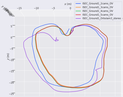
(a)

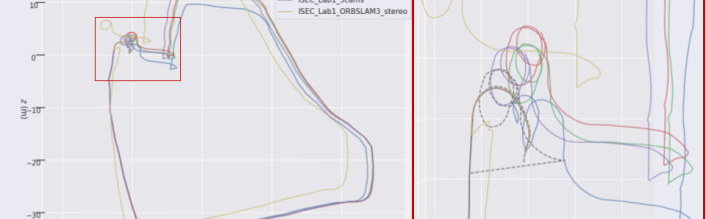
(b)

Figure 5: Estimated trajectories of the proposed generic SLAM system and ORBSLAM3 for ISEC_Ground1(a) and ISEC_Lab1 (b) sequences. In (b) the ground truth is the dashed line. For ISEC_Ground1 sequence(a) the start and end positions of the robot are the same which helps us to measure performance. In the stereo setup, we outperform ORBSLAM3 which experiences incorrect tracking caused by dynamic objects encountered along the trajectory. The trials associated with our method show an improvement in the accuracy of the estimated trajectory as we increase the number of overlapping cameras.

Quantitative results: From table II we can observe that with a stereo setup our method exhibits more accuracy when compared to ORBSLAM3 in four out of the five datasets. While the error difference is not much for ISEC_Lab1, ISEC_Ground1, and ISEC_Ground2 trajectories, it is significant for the Curry_center trajectory, which is both longer and has much more dynamic content with people moving around on the Northeastern University campus. In the Falmouth sequence, which features off-road outdoor images with dried foliage we perform poorly compared to ORBSLAM3 in the stereo configuration. We disabled loop closing in ORBSLAM3 in the comparisons to accurately compute the accumulated drift. With the loop closing ORBSLAM3’s estimates improve. However, for really long trajectories like the Falmouth sequence, we observed that even with loop closing ON ORBSLAM3 could not recover from the accumulated drift.

VII-B Effect of Camera Configuration

Along with comparing our method with a state-of-the-art SLAM system, we also evaluate and discuss the effect of the following parameters on the performance of the proposed SLAM pipeline.

VII-B1 Accuracy

Number of Cameras: Within the overlapping configuration we evaluate our method by choosing a subset of cameras, and increasing the number of cameras for each trial. We start with 2 cameras with the smallest baseline and go up to 5 cameras in the front-facing array. TableII shows that within each sequence, the ATE decreases as the number of overlapping cameras increases. We can see the same trend in the trajectory plots shown in fig. 5(a), fig. 5(b) and fig. 6. The estimated trajectory is closer to the ground truth as we increase the number of cameras. This can be clearly observed in the zoomed portion of the trajectory in fig. 5(b).

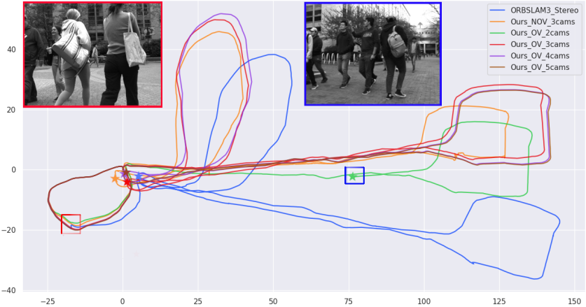
Figure 6: Estimated trajectories of the Curry_center sequence that has outdoor data with heavy dynamic content. The stars indicate the final positions of the trajectory estimates. With overlapping camera configurations, the accuracy of SLAM estimates increases with the number of cameras as indicated by the accumulated drift in the final position. We show the tracking failures on the trajectories caused due to occluding dynamic objects by highlighting the imagery at those points, with red and blue boxes. The non-overlapping configuration demonstrates scale issues when compared to the OV configuration with the same number of cameras but is robust to dynamic content.

Overlap vs Non-Overlap: Here, we compare the tracking accuracy between a set of overlapping cameras chosen from the front-facing array, and a set of non-overlapping cameras facing different directions with the same number of cameras(N=3), as shown in fig. 4. From tableII errors for the non-overlapping configuration are always more than the overlapping configuration with the same number of cameras. This is because the non-overlapping setup quickly accumulates scale drift. The error is particularly high in the ISEC_Lab1 sequence, which has narrow featureless corridors and reflective glass walls rendering the sideward-looking cameras useless for tracking.

VII-B2 Robustness:

In addition to measuring accuracy we also study the robustness of tracking across different camera configurations. To do this we take a closer look at multiple runs of the SLAM pipeline for Curry_center sequence which is a large dataset(597m) that features heavy dynamic content as shown in fig. 6. This data was collected by navigating the robot around the Northeastern University campus on a regular working day while there was a lot of human activity. Figure6 shows the best run for each camera configuration for simplicity. The red and blue boxes indicate the places on the trajectories when we experience tracking failures and the corresponding images acquired by one of the cameras is displayed. In our runs, we experience the highest number of tracking failures in the two-camera (stereo) overlapping configuration. The tracking failures also happen in the three-camera overlapping configuration but is not as frequent as in the two-camera case. The overlapping configuration with 4 and 5 cameras runs successfully, following each other very closely. The non-overlapping 3 camera configuration does not fail in the presence of dynamic objects because when one view is occluded, it has the support of the other views to track features. However, the trajectory estimates are inaccurate and exhibit severe scale errors.

VII-C Run Time Performance

We conclude the evaluation by measuring the average time taken to process a single multi-camera frame. TableIII shows the average time taken for various camera configurations for the Curry_center sequence. Individual processing times for feature extraction, tracking and mapping, back-end optimization modules, and the total processing time per frame are reported separately in milliseconds. The results show that the processing time increases with the number of cameras in the overlapping configuration as expected because we have the extra burden of computing multi-view features between component cameras in the front end. The computational load in the back end also increases due to increased observations. We can achieve a maximum processing speed of 19.1 fps for a stereo configuration and a minimum of 11.45 fps for five cameras in the overlapping configuration.

Average Time Taken for Processing (Milli Seconds)
	2 cams	3cams	4cams	5cams	N-OV
Feature Extraction	23.1	25.61	29.16	32.64	21.3
Tracking & Mapping	8.02	8.64	9.85	10.78	8.32
Optimization	10.23	20.7	27.02	31.83	10.99
Total Avg time	52.14	64.91	74.89	87.33	58.08

TABLE III: Run time performance of our method. We show the average time taken for different steps in the pipeline - feature extraction, tracking and mapping, optimization and the total time per frame. The processing time clearly increases with number of cameras. We can run at 11 fps for the five-camera configuration which is close to real-time.

VIII Conclusion

We presented a generic multi-camera SLAM framework that can adapt to any arbitrary camera system configuration. The core contribution of this paper is the camera configuration independent design and real-time implementation across the complete SLAM pipeline. We leverage the camera geometry to extract well distributed multi-view features by effectively utilizing the overlapping FoVs among cameras. We conducted extensive evaluations on real-world datasets collected using a custom-built camera rig featuring a variety of challenging conditions. We also benchmark the performance of the SLAM pipeline in terms of the number of cameras and the overlap information that define the camera configuration. This analysis can be used in designing multi-camera systems for accurate and robust SLAM. This work addresses the gap between the state of the art visual SLAM algorithms and their applicability to real-world deployments of multi-camera systems. We make the code and datasets publicly available to foster research in this direction.

References

- [1] A. J. Davison, “Real-time simultaneous localisation and mapping with a single camera,” in Computer Vision, IEEE International Conference on, vol. 3. IEEE Computer Society, 2003, pp. 1403–1403.
- [2] J. Engel, J. Stückler, and D. Cremers, “Large-scale direct SLAM with stereo cameras,” in 2015 IEEE/RSJ international conference on intelligent robots and systems (IROS). IEEE, 2015, pp. 1935–1942.
- [3] C. Campos, R. Elvira, J. J. G. Rodríguez, J. M. Montiel, and J. D. Tardós, “ORBSlam3: An Accurate Open-Source Library for Visual, Visual–Inertial, and Multimap SLAM,” IEEE Transactions on Robotics, 2021.
- [4] J. Kuo, M. Muglikar, Z. Zhang, and D. Scaramuzza, “Redesigning slam for arbitrary multi-camera systems,” in 2020 IEEE International Conference on Robotics and Automation (ICRA). IEEE, 2020.
- [5] R. A. Newcombe, S. J. Lovegrove, and A. J. Davison, “DTAM: Dense tracking and mapping in real-time,” in 2011 international conference on computer vision. IEEE, 2011, pp. 2320–2327.
- [6] C. Kerl, J. Sturm, and D. Cremers, “Robust odometry estimation for RGB-D cameras,” in 2013 IEEE international conference on robotics and automation. IEEE, 2013, pp. 3748–3754.
- [7] D. Scaramuzza and R. Siegwart, “Appearance-guided monocular omnidirectional visual odometry for outdoor ground vehicles,” IEEE transactions on robotics, vol. 24, no. 5, pp. 1015–1026, 2008.
- [8] D. Caruso, J. Engel, and D. Cremers, “Large-scale direct SLAM for omnidirectional cameras,” in 2015 IEEE/RSJ International Conference on Intelligent Robots and Systems (IROS). IEEE, 2015, pp. 141–148.
- [9] H. Matsuki, L. Von Stumberg, V. Usenko, J. Stückler, and D. Cremers, “Omnidirectional DSO: Direct sparse odometry with fisheye cameras,” IEEE Robotics and Automation Letters, vol. 3, no. 4, 2018.
- [10] C. Forster, M. Pizzoli, and D. Scaramuzza, “SVO: Fast semi-direct monocular visual odometry,” in 2014 IEEE international conference on robotics and automation (ICRA). IEEE, 2014, pp. 15–22.
- [11] J. Sola, A. Monin, M. Devy, and T. Vidal-Calleja, “Fusing monocular information in multicamera SLAM,” IEEE transactions on robotics, vol. 24, no. 5, pp. 958–968, 2008.
- [12] M. Kaess and F. Dellaert, “Probabilistic structure matching for visual SLAM with a multi-camera rig,” Computer Vision and Image Understanding, vol. 114, no. 2, pp. 286–296, 2010.
- [13] S. Urban and S. Hinz, “Multicol-slam-a modular real-time multi-camera slam system,” arXiv preprint arXiv:1610.07336, 2016.
- [14] R. Pless, “Using many cameras as one,” in 2003 IEEE Computer Society Conference on Computer Vision and Pattern Recognition, 2003. Proceedings., vol. 2. IEEE, 2003, pp. II–587.
- [15] Z. Zhang and K. Zou, “MMO-SLAM: A Versatile and Accurate Multi Monocular SLAM System,” Journal of Intelligent & Robotic Systems, vol. 105, no. 3, pp. 1–23, 2022.
- [16] M. J. Tribou, A. Harmat, D. W. Wang, I. Sharf, and S. L. Waslander, “Multi-camera parallel tracking and mapping with non-overlapping fields of view,” International Journal of Robotics Research, vol. 34, no. 12, 2015.
- [17] G. Carrera, A. Angeli, and A. J. Davison, “Lightweight SLAM and Navigation with a Multi-Camera Rig,” European Conference on Mobile Robots, pp. 77–82, 2011.
- [18] S. Houben, J. Quenzel, N. Krombach, and S. Behnke, “Efficient multi-camera visual-inertial SLAM for micro aerial vehicles,” IEEE International Conference on Intelligent Robots and Systems, vol. 2016-Novem, no. October, pp. 1616–1622, 2016.
- [19] L. Heng, G. H. Lee, and M. Pollefeys, “Self-calibration and visual slam with a multi-camera system on a micro aerial vehicle,” Autonomous robots, vol. 39, no. 3, pp. 259–277, 2015.
- [20] H. Seok and J. Lim, “Rovo: Robust omnidirectional visual odometry for wide-baseline wide-fov camera systems,” in 2019 International Conference on Robotics and Automation (ICRA). IEEE, 2019.
- [21] J. Jaekel, J. G. Mangelson, S. Scherer, and M. Kaess, “A robust multi-stereo visual-inertial odometry pipeline,” IEEE International Conference on Intelligent Robots and Systems, pp. 4623–4630, 2020.
- [22] P. Liu, M. Geppert, L. Heng, T. Sattler, A. Geiger, and M. Pollefeys, “Towards Robust Visual Odometry with a Multi-Camera System,” IEEE International Conference on Intelligent Robots and Systems, 2018.
- [23] L. Heng, B. Choi, Z. Cui, M. Geppert, S. Hu, B. Kuan, P. Liu, R. Nguyen, Y. C. Yeo, A. Geiger, G. H. Lee, M. Pollefeys, and T. Sattler, “Project autovision: Localization and 3D scene perception for an autonomous vehicle with a multi-camera system,” arXiv, 2018.
- [24] P. Kaveti, J. S. Nir, and H. Singh, “Towards robust vslam in dynamic environments: A light field approach,” in 2021 IEEE International Conference on Multisensor Fusion and Integration for Intelligent Systems (MFI). IEEE, 2021.
- [25] A. Li, D. Zou, and W. Yu, “Robust initialization of multi-camera slam with limited view overlaps and inaccurate extrinsic calibration,” in 2021 IEEE/RSJ International Conference on Intelligent Robots and Systems (IROS). IEEE, 2021, pp. 3361–3367.
- [26] L. Zhang, D. Wisth, M. Camurri, and M. Fallon, “Balancing the budget: Feature selection and tracking for multi-camera visual-inertial odometry,” IEEE Robotics and Automation Letters, vol. 7, no. 2, 2021.
- [27] Z. Zhang, H. Rebecq, C. Forster, and D. Scaramuzza, “Benefit of large field-of-view cameras for visual odometry,” in 2016 IEEE International Conference on Robotics and Automation (ICRA). IEEE, 2016.
- [28] K. Chappellet, G. Caron, F. Kanehiro, K. Sakurada, and A. Kheddar, “Benchmarking cameras for open vslam indoors,” in 2020 25th International Conference on Pattern Recognition (ICPR). IEEE, 2021.
- [29] H. Li, R. Hartley, and J.-h. Kim, “A linear approach to motion estimation using generalized camera models,” in 2008 IEEE Conference on Computer Vision and Pattern Recognition. IEEE, 2008, pp. 1–8.
- [30] L. Kneip, H. Li, and Y. Seo, “Upnp: An optimal o (n) solution to the absolute pose problem with universal applicability,” in European conference on computer vision. Springer, 2014, pp. 127–142.
- [31] F. Dellaert, M. Kaess, et al., “Factor graphs for robot perception,” Foundations and Trends® in Robotics, vol. 6, no. 1-2, 2017.
- [32] P. Furgale, J. Rehder, and R. Siegwart, “Unified temporal and spatial calibration for multi-sensor systems,” in 2013 IEEE/RSJ International Conference on Intelligent Robots and Systems. IEEE, 2013.