Transition from Susceptible-Infected to Susceptible-Infected-Recovered Dynamics in a Susceptible-Cleric-Zombie-Recovered Active Matter Model

Abstract

The Susceptible-Infected (SI) and Susceptible-Infected-Recovered (SIR) models provide two distinct representations of epidemic evolution, distinguished by the lack of spontaneous recovery in the SI model. Here we introduce a new active matter epidemic model, the “Susceptible-Cleric-Zombie-Recovered” (SCZR) model, in which spontaneous recovery is absent but zombies can recover with probability $\gamma$ via interaction with a cleric. Upon interacting with a zombie, both susceptibles and clerics can enter the zombie state with probability $\beta$ and $\alpha$, respectively. By changing the intial fraction of clerics or their healing ability rate $\gamma$, we can tune the SCZR model between SI dynamics, in which no susceptibles or clerics remain at long times, and SIR dynamics, in which no zombies remain at long times. The model is relevant to certain real world diseases such as HIV where spontaneous recovery is impossible but where medical interventions by a limited number of caregivers can reduce or eliminate the spread of infection.

I Introduction

Understanding the propagation of infectious diseases is an intensely studied issue, and a variety of different epidemic models and methods to simulate the spread of disease have been developed Kermack and McKendrick (1927); Bailey (1975); Hethcote (2000); Martcheva (2015). Two of the most widely used disease propagation models are the Susceptible-Infected (SI) and Susceptible-Infected-Recovered (SIR) models Kermack and McKendrick (1927); Bailey (1975); Hethcote (2000); Martcheva (2015). In the SI model, illustrated in Fig. 1(a), there are only susceptibles ($S$) and infectives ($I$) present. There is no spontaneous recovery, and the model contains only a single probability $\beta$ for an $S$ to transform to an $I$. As shown in Fig. 1(b), the SIR model adds a spontaneous recovery process with rate $\mu$ for an $I$ to become recovered ($R$). A key difference between the SI and SIR models is that in the SI model the amount of $S$ present drops to zero at long times, but in the SIR model the amount of $I$ present drops to zero. A wide range of diseases can be described using these two models. Diseases with lifelong transmittivity and no recovery are captured by the SI model, while situations where reinfection is impossible but spontaneous recovery occurs can be represented with the SIR model. Numerous variations of the SI and SIR models have been considered over the years Bailey (1975); Hethcote (2000); Martcheva (2015); Bjørnstad et al. (2020), including epidemic spreading on networks Pastor-Satorras et al. (2015), memory effects Bestehorn et al. (2022), adding vaccination Gao et al. (2007), spatial heterogeneity Keeling (1999); Tildesley et al. (2009), social distancing te Vrugt et al. (2020), diffusion Polovnikov et al. (2022), and models that include details on mobility patterns in attempts to more accurately portray real world epidemics Eubank et al. (2004); Germann et al. (2006).

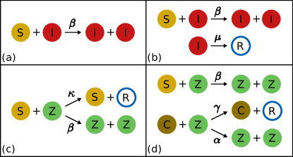
Figure 1: (a) In the SI model, there is no spontaneous recovery, and susceptibles ($S$, yellow) that come into contact with infectives ($I$, red) become infected with probability $\beta$. (b) The SIR model adds a spontaneous recovery process in which an $I$ transitions to recovered ($R$, blue open circle) at a rate $\mu$. (c) In the Living-Zombie-Recovered model introduced in Ref. Alemi et al. (2015), a zombie ($Z$, green) interacting with $S$ recovers with probability $\kappa$ and turns the $S$ into $Z$ with probability $\beta$. (d) In our SCZR model, we divide the susceptible population into $S$ and clerics ($C$, brown). $Z$ can only recover when in contact with $C$ with probability $\gamma$, but interaction with $Z$ causes $S$ to turn into $Z$ with probability $\beta$ and $C$ to turn into $Z$ with probability $\alpha$.

Despite the large number of models that have been explored, we did not find any descriptions of a model in which a transition from SI to SIR behavior naturally emerges. Such transitions could arise for certain types of infectious disease where spontaneous recovery does not occur but where direct medical intervention can result in recovery or a reduced rate of infectiousness. For example, in the human immunodeficiency virus (HIV), an untreated patient remains contagious, but when appropriate medical interventions are applied, the patient becomes effectively cured and has a rate of infectiousness that drops dramatically or even reaches zero. In such cases, if there is an insufficient supply of resources or treating agents (doctors), the course of the epidemic will follow the SI model, but if there are ample resources or treating agents, the epidemic will instead fall in the SIR regime.

Standard SI and SIR type models assume homogeneous mixing of infectious and susceptible individuals, either across the entire population or within strata. For many diseases, that assumption is known to fail and in Refs. Burr and Chowell (2008); Großmann et al. (2021), the impact of the failure of the homogeneity assumption is studied. In our previous work Forgács et al. (2022), we showed that a run-and-tumble active matter model combined with SIR dynamics produces different regimes of behavior when quenched disorder is introduced, due to the lack of homogeneous mixing in the system. For low infection rates, the quenched disorder strongly affects the duration of the epidemic as well as the final epidemic size or fraction of $S$ that survive to the end of the epidemic. When the infection rate is high, the quenched disorder has little impact and the epidemic propagates as waves through the system.

The term “active matter” encompasses self driven systems such as an assembly of self-motile particles that undergo contact interactions with each other Marchetti et al. (2013); Bechinger et al. (2016). In our previous work Forgács et al. (2022), we considered run-and-tumble particles moving in two dimensions and subjected to rules of how an infection spreads when a contact interaction occurs between an $S$ and an $I$ particle. Active matter systems are attractive for epidemic modeling since they allow real world effects such as spatial heterogeneity to be incorporated easily because density heterogeneities arise naturally from the interactions among the particles, and there have now been several studies in which active matter is used to study epidemics Paoluzzi et al. (2020); Norambuena et al. (2020); Zhao et al. (2022). There have also been several experimental realizations of active matter systems that can mimic social dynamics through the activity and tracking of individual active particles, so the type of active matter epidemic systems we consider here should be feasible to create experimentally Lavergne et al. (2019); Bäuerle et al. (2020).

Here we introduce a new model for epidemic spreading featuring multiple susceptible species and no spontaneous recovery, and show that in this model, an easily tunable transition between SI and SIR behavior occurs. We specifically consider a modification of the Susceptible-Zombie-Removed (SZR) model proposed by Alemi et al. Alemi et al. (2015). Figure 1(c) shows the dynamics of the SZR model. Unlike the SIR model, the SZR model has no spontaneous recovery. Instead, when an $S$ and a zombie ($Z$) interact, the $Z$ transitions to recovered ($R$) with probability $\kappa$, while the $S$ transitions to $Z$ with probability $\beta$. In our modification of the model, there is again no spontaneous recovery, but we break the susceptible population into two portions: susceptibles ($S$) and clerics ($C$). As illustrated in Fig. 1(d), when an $S$ interacts with a $Z$, the $S$ becomes a $Z$ with probability $\beta$, as in the SZR model; however, the $S$ cannot cause the $Z$ to recover. Instead, only an interaction between a $C$ and a $Z$ can cause the $Z$ to recover with probability $\gamma$, while with probability $\alpha$, the $C$ becomes a $Z$. We call this the Susceptible-Cleric-Zombie-Removed or “SCZR” model. Although, as in Ref. Alemi et al. (2015), we have placed the model in a zombie framework, the model can be rephrased in terms of certain real world diseases such as HIV which, if left untreated, confer a lifelong ability to infect; however, under medical treatment from a health care provider, the infection rate can be reduced or dropped to zero, resulting in an effectively recovered individual. In this case, the zombie class would be simply be labeled as infected ($I$) while the cleric class would represent some form of health care provider or medical resources. As we show below, the SCZR model exhibits SI behavior when the initial fraction of $C$ or the healing rate $\gamma$ is low, since in this case the $Z$ wipe out both the $C$ and the $S$ so that a finite fraction of $Z$ remain at the end of the epidemic. In contrast, when the initial fraction of $C$ or the healing rate $\gamma$ is high enough, the $C$ are able to eliminate the $Z$ so that a finite fraction of $S$ and $C$ remain at the end of the epidemic, which is behavior associated with an SIR model.

II Modeling and characterization of the SCZR dynamics

We consider a two-dimensional assembly of $N=5000$ run-and-tumble active particles in a system of size $L\times L$ where $L=200.0$ and where there are periodic boundary conditions in both the $x$ and $y$ directions. The motion of the particles is obtained by integrating the following overdamped equation of motion in discrete time:

$$\alpha_{d}{\bf v}_{i}={\bf F}^{dd}_{i}+{\bf F}^{m}_{i}\ .$$ (1)

Here ${\bf v}_{i}={d{\bf r}_{i}}/{dt}$ is the velocity and ${\bf r}_{i}$ is the position of particle $i$, and the damping constant $\alpha_{d}=1.0$. The interaction between two particles, each of radius $r_{a}=1.0$, is modeled with a harmonic repulsive potential ${\bf F}^{dd}_{i}=\sum_{i\neq j}^{N}k(2r_{a}-|{\bf r}_{ij}|)\Theta(|{\bf r}_{ij}|-2r_{a}){\hat{\bf r}_{ij}}$, where $\Theta$ is the Heaviside step function, ${\bf r}_{ij}={\bf r}_{i}-{\bf r}_{j}$, $\hat{\bf r}_{ij}={\bf r}_{ij}/|{\bf r}_{ij}|$, and the repulsive spring force constant is $k=20.0$.

Each particle is subjected to an active motor force ${\bf F}_{i}^{m}=F_{M}{\bf\hat{m}}_{i}$ of magnitude $F_{M}$ applied in a randomly chosen direction ${\bf\hat{m}}_{i}$ during a continuous run time of $\tau_{l}\in[1.5\times 10^{4}$, $3.0\times 10^{4}]$ before instantaneously changing to a new randomly chosen direction. This type of run-and-tumble dynamics of active particles has been used extensively to model active matter systems Marchetti et al. (2013); Bechinger et al. (2016); Cates and Tailleur (2015), active ratchets Reichhardt and Reichhardt (2017), active jamming Reichhardt and Olson Reichhardt (2014) and motility induced phase separation Cates and Tailleur (2015); Sándor et al. (2017). In another version of active matter, the particles undergo driven diffusion; however, many of the generic phases are the same for both run-and-tumble and driven diffusive active matter Cates and Tailleur (2015, 2013), so we expect that our results will also be relevant to driven diffusive systems. For sufficiently large density or activity, both run-and-tumble and driven diffusive active particles begin to exhibit self-clustering, leading to what is known as motility-induced phase separation (MIPS) Marchetti et al. (2013); Bechinger et al. (2016); Cates and Tailleur (2015); Fily and Marchetti (2012); Redner et al. (2013); Palacci et al. (2013); Buttinoni et al. (2013).

We select the run length range and motor force value such that the system is in the MIPS regime, and thus creates large connected active clusters similar to those employed in our previous active matter epidemic model Forgács et al. (2022). Each particle tracks which one of the four possible states, $S$, $Z$, $C$ or $R$, it is currently occupying. These states are linked together by the following equations:

$$dS =-\beta SZ$$ (2)

$$dZ =\alpha CZ+\beta SZ-\gamma CZ$$ (3)

$$dC =-\alpha CZ$$ (4)

$$dR =\gamma CZ\ .$$ (5)

According to these equations, when an $S$ particle encounters a $Z$ particle, it changes its label to $Z$ with rate $\beta$. More interestingly, when a C and Z particle come in contact, a change in state occurs with rate $\alpha+\gamma$. For interactions in which a state change occurs, with probability $\alpha/(\alpha+\gamma)$ the $C$ particle becomes a $Z$, and with probability $\gamma/(\alpha+\gamma)$, the $Z$ morphs into $R$. Our simulation discretizes time in $\Delta$-sized steps, and in the above dynamic, rates are changed into probabilities. Specifically, the probability that an $S$ particle in contact with a $Z$ particle morphs into a $Z$ particle is $1-e^{-\Delta\beta}$. Similarly, the probability that a change occurs during a $Z$ and $C$ particle encounter is $1-e^{-\Delta(\alpha-\gamma)}$. The probability of transitions from $C$ to $Z$ and $Z$ to $R$ remains unchanged.

If at a given time step an $S$ particle is in contact with multiple $Z$ particles, or a $Z$ particle is in contact with multiple $C$ or $S$ particles, every possible pair interaction is computed independently using the unmodified states of all particles, and the state of each particle is updated simultaneously at the end of the computation when we apply all $S\rightarrow Z$, $Z\rightarrow R$, and $C\rightarrow Z$ transitions. There are no concurrency issues since each type of particle can undergo only one type of transition.

The $R$ state is absorbing since the $R$ particles experience no further state transitions, but there is no mechanism to replenish the initial pool of either $S$ or $C$ particles. The epidemic ends when either there are no more $S$ and $C$ particles or there are no more $Z$ particles. Therefore, there are only two possible types of final state for the SCZR model: an SI-like situation in which all $S$ and $C$ particles have been transformed into $Z$ and $R$ particles (indicating that the zombies or the clinical cases prevail), and an SIR-like situation in which all $Z$ particles have been extinguished by becoming $R$ particles (indicating that the medical community prevails and no zombies or clinical cases remain). While the time $t_{d}$ to reach the final state is finite, we observe in simulations that $t_{d}$ can become very long because, in order for the epidemic to come to a conclusion, it is necessary for the remaining $S$ and $C$ or the remaining $Z$ particles to come into contact with $Z$ or $C$ particles, respectively.

We initialize the system by randomly placing the particles at non-overlapping positions in the sample. Initially all of the particles are set to the S state. We allow the system to evolve for $5\times 10^{5}$ simulation time steps until a large MIPS cluster emerges, and we define this state to be the $t=0$ condition. We then randomly select five particles and change their state to $Z$. We choose five particles rather than one particle in order to lower the probability of a failed outbreak. We also randomly select a fraction ranging from $10\%$ to $100\%$ of the $S$ to change into $C$. The system continues to evolve under both the motion of the particles and the reactions between states $S$, $C$, $Z$, and $R$ until there are either no $S$ or $C$ particles or there are no $Z$ particles, indicating that further epidemiological change is impossible. We consider different values of $\alpha$, $\beta$, and $\gamma$ in addition to varying the fraction of $C$ in the initial population.

III Results

In Figure 2 we illustrate the spatial evolution of our system under the SCZR model at fixed $\alpha=5\times 10^{-6}$, $\beta=1\times 10^{-5}$ and $\gamma=1.9\times 10^{-5}$. For Fig. 2(a,b,c), the initial fraction of $C$ is $c_{0}\equiv C(t=0)/N=0.2$, and over time we find an SI-like behavior in which the zombie outbreak prevails and the populations of $S$ and $C$ drop to zero. When $c_{0}$ is raised to $c_{0}=0.4$, Fig. 2(d,e,f) shows an SIR-like behavior in which recovery prevails and the population of $Z$ drops to zero. The initial condition of the MIPS cluster is identical for the two cases, and the motion of the particles is not influenced by their epidemiological state. The peak of the zombie outbreak is shown in Figs. 2(b) and 2(e), and the particle positions are different for the two cases only because the peak in Fig. 2(e) occurs at a later time of $t=9.67\times 10^{5}$ compared to the peak in Fig. 2(b), which falls at $t=4.85\times 10^{5}$. In general we find that the progression of an SIR-like epidemic is significantly slower than that of an SI-like epidemic. The end state of the epidemic is illustrated in Fig. 2(c) when the last $C$ is eliminated after a time of $t=1.606\times 10^{6}$, and in Fig. 2(e) when the last $Z$ is eliminated after a time of $t=2.277\times 10^{6}$. In the well-mixed mean field limit, when $\beta>\alpha$ we would expect that all of the $S$ are eliminated prior to the elimination of the last $C$ for the $c_{0}=0.2$ system. In practice, due to the heterogeneity of our system, we found that out of all the SI simulations we considered, the $S$ were eliminated prior to the $C$ 78% of the time, and the $C$ were eliminated prior to the $S$ 22% of the time.

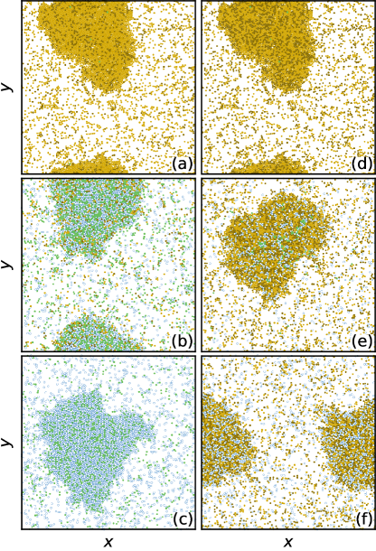
Figure 2: Snapshots of the time evolution of the SCZR system for $\alpha=5\times 10^{-6}$, $\beta=1\times 10^{-5}$, and $\gamma=1.9\times 10^{-5}$. Yellow disks are susceptibles ($S$), brown disks are clerics ($C$), green disks are zombies ($Z$), and open blue circles are recovered ($R$). (a,b,c) are for an initial cleric fraction of $c_{0}=0.2$, and (d,e,f) are for $c_{0}=0.4$. (a,d) The $t=0$ moment where the MIPS cluster is present. (b,e) The peak of the zombie outbreak, which occurs at $t=4.85\times 10^{5}$ in (b) and at $t=9.67\times 10^{5}$ in (e). (c,f) The final state, which is reached at $t=1.606\times 10^{6}$ in (c) and $t=2.277\times 10^{6}$ in (f). (a,b,c) show an SI-like evolution in which all $S$ and $C$ are eliminated in the final state, while (d,e,f) show an SIR-like evolution in which all $Z$ are eliminated in the final state.

In Fig. 3(a) we plot the epidemic curves $s=S/N$, $c=C/N$, $z=Z/N$, and $r=R/N$ versus simulation time for the $c_{0}=0.2$ system in the SI regime from Fig. 2(a,b,c). At first, $r$ and $z$ increase at roughly the same rate until $z$ passes through a local peak. Meanwhile, since $\beta>\alpha$, $s$ decreases more rapidly than $c$, and at longer times $z$ undergoes a modest decrease from its peak value so that, at the end of the epidemic, $s=0$, $c=0$, $z=0.25$, and $r=0.75$. Figure 3(b) shows the epidemic curves for the SIR regime with $c_{0}=0.4$ from Fig. 2(d,e,f). Here the evolution to the final state occurs much more slowly, and in order to show the behavior of $z$ clearly we plot $z$ on a separate $y$ axis scale, which is why the curve has a noisy appearance. Both $s$ and $c$ decrease with time, but after passing through a peak, $z$ drops to $z=0$ at the end of the epidemic while the values of $s$, $c$, and $r$ all remain finite. At late times during the epidemic in Fig. 3(b), where all of the epidemic curves become relatively flat, a strongly stochastic process occurs in which the surviving $C$ and $Z$ need to come into contact with each other in order to end the epidemic. Since the motion of both $C$ and $Z$ is diffusive in nature, this slows the progression of the epidemic and introduces more stochasticity. For late times in Fig. 3(a), as the surviving $Z$ transform the remaining $C$ into $Z$, $z$ increases with each transformation and so there is a higher probability of making contact with the remaining $C$, shortening the epidemic. In contrast, for late times in Fig. 3(b), the surviving $C$ transform the remaining $Z$ into $R$, which are epidemiologically inert, so there is no increase in $c$ with each transformation and the total duration $t_{d}$ of the epidemic is longer.

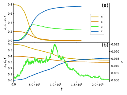
Figure 3: Epidemic curves for the individual runs illustrated in Fig. 2 with $\alpha=5\times 10^{-6}$, $\beta=1\times 10^{-5}$ and $\gamma=1.9\times 10^{-5}$ showing the fractions of susceptible $s$ (yellow), cleric $c$ (brown), zombie $z$ (green), and recovered $r$ (blue) particles versus time $t$. (a) SI-like progression at $c_{0}=0.2$ corresponding to the system in Fig. 2(a,b,c). Here, $s=c=0$ in the final state. (b) SIR-like progression at $c_{0}=0.4$ corresponding to the system in Fig. 2(d,e,f). The value of $z$ is plotted on a separate $y$ axis for better visibility. In the final state, $z=0$.

We next consider how changing the values of the model parameters $c_{0}$, $\alpha$, $\beta$, and $\gamma$ affects the epidemic outcomes. To characterize the outcome of a given simulation, we introduce the quantity

$$\upsilon=(s_{f}+c_{f})/(s_{0}+c_{0}),$$ (6)

where $s_{0}=S(t=0)/N$ is the initial fraction of susceptibles, $s_{f}=S(t=t_{d})/N$ is the final fraction of susceptibles at time $t=t_{d}$ equal to the duration of the epidemic, and $c_{f}=C(t=t_{d})/N$ is the final fraction of clerics. Using $\upsilon$ we can determine what fraction of the initial population of $S$ and $C$ survive the epidemic. In the SI-like regime, $\upsilon=0$, and in the SIR-like regime, $\upsilon$ remains finite.

From an epidemiological point of view, $\upsilon$ gives an indication of how effective the medical intervention by the clerics is at suppressing the epidemic. High values of $\upsilon$ are desirable since this indicates that a smaller fraction of the population caught the disease. For any individual simulation with a given set of parameters, it is possible to have either SI or SIR behavior emerge due to the stochasticity, so we average $\upsilon$ over an ensemble of 50 runs for each parameter choice, where each run has a different random seed for the initial particle positions and placement of $Z$ and $C$ particles. When $\langle\upsilon\rangle$ remains high, the SIR behavior is dominant and the $Z$ are usually eliminated from the system, while when $\langle\upsilon\rangle$ becomes small, the SI behavior is dominant and the $S$ and $C$ are usually eliminated from the system so that the zombies prevail.

In Fig. 4 we plot phase diagrams of $\upsilon$ as a function of $c_{0}$, the initial cleric fraction, versus $\gamma$, the probability of the transition $C+Z\rightarrow C+R$. Each diagram contains 160 points, and each point is averaged over 50 different initial realizations. In the blue region, $\upsilon$ is high and we find SIR-like behavior where $S$ and $C$ survive while $Z$ are eliminated, while in the green region, $\upsilon$ is low and the system is SI-like, with $Z$ persisting to the end of the epidemic and all of the $S$ and $C$ vanishing. Figure 4(a) shows the phase diagram for samples with $\alpha=5\times 10^{-6}$ and $\beta=1\times 10^{-5}$, as in Figs. 2 and 3. At higher $\gamma$, the zombies are more effectively healed by the clerics, and the initial fraction $c_{0}$ of $C$ needed to produce SIR-like behavior drops to lower values, as shown by the solid line which is a fit of the SI-SIR transition to the form $c_{0}\propto a(\gamma+b)^{-1}$. For a simple way to understand the general form of this curve, consider the early time behavior of an individual $Z$ particle. As it moves, the $Z$ encounters a $C$ with probability $c_{0}$ and an $S$ with probability $1-c_{0}$. The $Z$ always survives an encounter with $S$, but it only survives an encounter with $C$ with probability $1-\gamma$. Thus, the probability that the $Z$ survives is $Z_{\rm survive}=(1-\gamma)c_{0}+(1-c_{0})$ and the probability that the $Z$ is destroyed by turning into an $R$ is $Z_{\rm destroy}=\gamma c_{0}$. At the SI-SIR transition, we have $Z_{\rm survive}=Z_{\rm destroy}$, meaning that the transition line is expected to fall at $c_{0}=0.5(\gamma)^{-1}$.

The actual location of the SI-SIR transition line is affected by the values of $\alpha$ and $\beta$ because these control the way in which the populations of $S$, $C$, $Z$, and $R$ evolve over time. If we cut the probability $\alpha$ of the $C+Z\rightarrow Z+Z$ transition in half to $\alpha=2.5\times 10^{-6}$, the phase diagram in Fig. 4(b) indicates that the SI-SIR transition line shifts to lower values of $c_{0}$ since it becomes more difficult for the $Z$ to eliminate all of the $C$. If we instead double $\alpha$ to $\alpha=1\times 10^{-5}$, as in Fig. 4(c), we reach the limit in which $\alpha=\beta$ and the $S$ and $C$ particles are both equally likely to be infected upon encountering a $Z$. Here, not only does the SI-SIR transition line shift to higher $c_{0}$, but for small values of $\gamma$ only SI behavior can occur even if the entire population apart from the zombie index cases is initialized to state $C$. If we leave $\alpha$ unchanged but double $\beta$, the probability of the $S+Z\rightarrow Z+Z$ transition, to $\beta=2\times 10^{-5}$, Fig. 4(d) shows that at low $\gamma$, the location of the SI-SIR transition does not change very much, but at higher $\gamma$, it shifts to higher $c_{0}$.

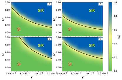
Figure 4: Phase diagrams showing heat maps of $\langle\upsilon\rangle$, the average fraction of the initial population of $S$ and $C$ that survive the epidemic, as a function of initial cleric fraction $c_{0}$ vs the probability $\gamma$ of the transition $C+Z\rightarrow C+R$. Blue indicates SIR behavior in which $Z$ are eliminated, and green indicates SI behavior in which $S$ and $C$ are eliminated. In general, as $\gamma$ increases, the SIR behavior emerges at a lower value of $c_{0}$. (a) Samples of the type shown in Figs. 1 to 3 with $\alpha=5\times 10^{-6}$ and $\beta=1\times 10^{-5}$. (b) Samples with the same $\beta=1\times 10^{-5}$ where $\alpha$, the probability for $C+Z\rightarrow Z+Z$, has been halved to $\alpha=2.5\times 10^{-6}$. (c) Samples with the same $\beta=1\times 10^{-5}$ in which $\alpha$ has been doubled to $\alpha=1\times 10^{-5}$. (d) Samples with the same $\alpha=5\times 10^{-6}$ in which $\beta$, the probability for $S+Z\rightarrow Z+Z$, is doubled to $\beta=2\times 10^{-5}$. The solid lines in the figures are fits of the form $c_{0}\propto a(\gamma+b)^{-1}$ where (a) $a=7.77\times 10^{-6}$ and $b=3.781\times 10^{-6}$, (b) $a=6.912\times 10^{-6}$ and $b=5.696\times 10^{-6}$, (c) $a=9.056\times 10^{-6}$ and $b=9.498\times 10^{-7}$, and (d) $a=1.212\times 10^{-5}$ and $b=8.381\times 10^{-6}$.

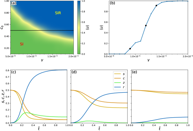
Figure 5: (a) The phase diagram with a heat map of $\langle\upsilon\rangle$ as a function of $c_{0}$ vs $\gamma$ from Fig. 4(a) with $\alpha=5\times 10^{-6}$ and $\beta=1\times 10^{-5}$. (b) A horizontal slice of $\langle\upsilon\rangle$ vs $\gamma$ taken at $c_{0}=0.5$ along the black line in panel (a). (c,d,e) Epidemic curves averaged over 50 runs taken at the black points in panel (b) showing $s$ (yellow), $c$ (orange), $z$ (green), and $r$ (blue) vs the rescaled time $\tilde{t}=t/t_{d}$. (c) At $\gamma=9\times 10^{-6}$, SI behavior occurs 90% of the time, so the averaged values of $s$ and $c$ do not reach zero but are lower than the averaged value of $z$. (d) At $\gamma=1.2\times 10^{-5}$, all runs are in the SIR regime and on average 50% of the population is never infected. (e) At $\gamma=1.4\times 10^{-5}$, the clerics become more effective at reducing the impact of the epidemic, and on average 90% of the population is never infected.

In order to illustrate some representative averaged epidemic curves, in Fig. 5(a) we reproduce the phase diagram of Fig. 4(a) for $\alpha=5\times 10^{-6}$ and $\beta=1\times 10^{-5}$ with a black line indicating the location of a horizontal cut. Figure 5(b) shows $\langle\upsilon\rangle$ versus $\gamma$ at the cut location of $c_{0}=0.5$. When $\gamma<9\times 10^{-6}$, there are no realizations in which SIR behavior occurs; instead, the $Z$ always wipe out all of the $S$ and $C$. Similarly, for $\gamma>1.1\times 10^{-5}$, there are no realizations in which SI behavior occurs, and the $Z$ are always fully eliminated. The kink in the curve marks the transition to fully SIR behavior. The value of $\langle\upsilon\rangle$ indicates how effective the clerics are at suppressing the epidemic. When $\langle\upsilon\rangle$ increases, it means that a greater fraction of the population was never infected by the disease. For $\gamma$ just above the transition into fully SIR behavior, over 75% of the population still becomes infected before the zombies are eliminated, whereas for higher $\gamma$, the majority of the population is able to avoid becoming infected.

For the three points highlighted in black in Fig. 5(b), we show averaged epidemic curves with $s$, $c$, $z$, and $r$ plotted as a function of normalized time $\tilde{t}=t/t_{d}$ in Figs. 5(c,d,e). For $\gamma=9\times 10^{-6}$ in Fig. 5(c), we are still in the SI dominated regime and the $z$ curve is higher than the $s$ and $c$ curves. Although in any individual run we either have $z=0$ or $s=c=0$, for the ensemble average $s$ and $c$ are finite since SIR behavior emerges 10% of the time. Since we are working at $c_{0}=0.5$, we have $s=c$ at the beginning of the epidemic, and although $s$ drops more rapidly than $c$ as the epidemic progresses, by the end of the epidemic $s\approx c$, due in large part to the many SI runs for which $s=c=0$. In Fig. 5(d) at $\gamma=1.2\times 10^{-5}$, all 50 simulations are in the SIR regime so that $z=0$ at the end of the epidemic, while the final value of $r\approx 0.5$ shows that on average half of the population becomes infected before the zombies are extinguished. Since we have $\beta=2\alpha$, the value of $s$ drops approximately twice as fast as the value of $c$ at early times in the epidemic, but as the supply of $Z$ is depleted through healing by the clerics, both $s$ and $c$ reach a plateau, and in the final state $c>s$. For $\gamma=1.9\times 10^{-5}$ in Fig. 5(e), well within the SIR regime, $z$ remains quite small throughout the epidemic. Although we still find $c>s$ at the end of the epidemic, both quantities have dropped only slightly from the original levels and are not very different from each other, and 90% of the population is able to avoid becoming infected.

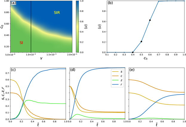
Figure 6: The phase diagram with a heat map of $\langle\upsilon\rangle$ as a function of $c_{0}$ vs $\gamma$ from Fig. 4(a) with $\alpha=5\times 10^{-6}$ and $\beta=1\times 10^{-5}$. (b) A vertical slice of $\langle\upsilon\rangle$ vs $c_{0}$ taken at $\gamma=1\times 10^{-5}$ along the black line in panel (a). (c,d,e) Epidemic curves averaged over 50 runs taken at the black points in panel (b) showing $s$ (yellow), $c$ (orange), $z$ (green), and $r$ (blue) vs $\tilde{t}$. (c) At $c_{0}=0.4$, only SI behavior occurs. (d) At $c_{0}=0.5$, we find mixed behavior, with an SI response occurring 36% of the time and an SIR response appearing in the remaining 64% of runs. (e) At $c_{0}=0.6$, all runs are in the SIR regime.

As shown in Fig. 6(a), we next consider a vertical cut at $\gamma=1\times 10^{-5}$ from the phase diagram in Fig. 4(a) for $\alpha=5\times 10^{-6}$ and $\beta=1\times 10^{-5}$. In Fig. 6(b) we plot $\langle\upsilon\rangle$ versus $c_{0}$ along this cut. For $c_{0}<0.5$, all of the realizations are in the SI regime and the $Z$ prevail, while for $c_{0}\geq 0.6$, all of the realizations are in the SIR regime and there are no $Z$ remaining at the end of the epidemic. The black points in Fig. 6(b) correspond to the values of $c_{0}$ at which the averaged epidemic curves in Figs. 6(c,d,e) were obtained. At $c_{0}=0.4$ in the SI regime, Fig. 6(c) shows that at the end of the epidemic, $s=c=0$ and the average fraction of zombies is $z=0.28$. When $c_{0}=0.5$ in Fig. 6(d), the system is in the SI regime 36% of the time, so that the final value of $z$ is greater than zero. Although $c$ and $s$ approach each other toward the end of the epidemic, we find that $c>s$ by a small amount since the $s=c=0$ behavior of the SI regime is no longer dominant. In Fig. 6(e), for $c_{0}=0.6$ the system is fully in the SIR regime, and throughout the epidemic we find not only that $c>s$ but that the difference between $c$ and $s$ remains constant. This is an indication of the importance of the stochastic diffusive process that occurs in our model in order to permit $Z$ to come into contact with $S$ or $C$. For $c_{0}=0.4$ in Fig. 6(c), at early times in the epidemic a $Z$ encounters an $S$ 60% of the time but a $C$ only 40% of the time. Since $S$ are twice as likely as $C$ to be infected, $s$ drops much more rapidly than $c$ in this regime. When $c_{0}$ is increased to $c_{0}=0.5$ in Fig. 6(d), a $Z$ is equally likely to encounter an $S$ or a $C$ at early times, and we see that the doubled infection probability causes $s$ to drop about twice as fast as $c$, as also shown in Fig. 5(c,d,e). Further increasing $c_{0}$ to $c_{0}=0.6$ in Fig. 6(e) means that at early times a $Z$ encounters a $C$ 60% of the time and an $S$ only 40% of the time. Since the $C$ are more resistant to infection, the relative fraction of $C$ and $S$ in the population remains nearly constant. Increasing $c_{0}$ even further produces many short-lived epidemics in which $s$ and $c$ do not change very much from their initial values.

We can analytically evaluate $\upsilon$ for well mixed systems whose dynamics is described through Equations (2)-(5). Using a standard argument (see JC (2012)) and some algebra, we can show that

$$\left(\frac{s}{s_{0}}\right)^{\alpha}=\left(\frac{c}{c_{0}}\right)^{\beta}$$

This provides us with the opportunity to compute a target for $\upsilon$:

$$\upsilon=(s_{f}+c_{0}(s_{f}/s_{0})^{\alpha/\beta})/(s_{0}+c_{0})\ .$$

Failure to hit that target in simulations is an indication that the homogeneous mixing assumption failed. From the data in Figs. 5(c,d,e) and 6(c,d,e), we find that the predicted value of $\upsilon$ is higher than the actual value of $\upsilon$, but that the agreement between predicted and actual improves as we move deeper into the SIR regime. This could be an indication that the SIR regime is better mixed than the SI regime, possibly due to the faster dynamics that tend to occur for SI behavior.

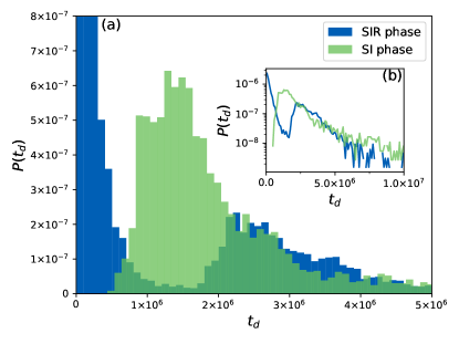
Figure 7: The distribution $P(t_{d})$ of epidemic durations for the runs presented in the phase diagrams of Fig. 4. Blue: runs in which the final state was in the SIR regime with all of the $Z$ eliminated. Green: runs in which the final state was in the SI regime with a finite population of $Z$ surviving at the end of the epidemic. Inset: The same data plotted on a log-linear scale.

In Fig. 7 we plot the distribution $P(t_{d})$ of the duration $t_{d}$ of the individual epidemics for the runs in all of the phase diagrams in Fig. 4. The data is split into two distributions, with the first for simulations that ended in the SI regime with a finite number of $Z$ remaining, and the second for simulations that ended in the SIR regime with no $Z$ remaining. For the SI case, there are no epidemics of short duration. This is because all $C$ and $S$ must be eliminated in the SI regime, and the elimination process requires a minimum amount of time to occur. In the inset we show the same data on a log-linear scale, indicating that some of the SI epidemics last for an extremely long time before reaching a final state. These lengthy epidemics occur for values of $c_{0}$ and $\gamma$ at which the behavior is evenly split between SI and SIR on average. There is also a peak in $P(t_{d})$ near $t_{d}=1.5\times 10^{5}$ simulation time steps. In the SIR regime, there is a large peak in $P(t_{d})$ at small $t_{d}$ corresponding to failed outbreaks in which the $C$ can rapidly encounter and cure the small number of $Z$ present at early times before the epidemic gets going. This is followed by a gap similar to what we observed previously in SIR simulations Forgács et al. (2022), and then by a second peak representing epidemics that involve a substantial portion of the population. Here we find that if the epidemic in the SIR regime is able to become established, it lasts longer than the typical epidemic in the SI regime, but that there is a high probability for the SIR epidemic to be extinguished before it can become established.

IV Discussion

As we noted earlier, although we have cast our SCZR model in terms of zombies and clerics, it could also be rephrased so that the zombies are disease-spreading individuals that cannot spontaneously recover from the disease they have caught, and the clerics are medical care providers who can cure the infected individuals or at least render them non-infectious. In this picture, when we take $\alpha<\beta$ but $\alpha>0$, this would mean that the medical care providers are more careful than the general population and take more precautions against becoming infected, but that they are not immune from becoming infected. The transition between SI and SIR behavior is significant because it indicates that by introducing a larger number of medical care providers (increasing $c_{0}$) or giving the medical care providers more effective treatment protocols (increasing $\gamma$), the disease can be prevented from entering the SI regime in which the entire population winds up getting infected eventually, and can instead be held in the SIR regime, ideally in the limit where $t_{d}$ is short and the epidemic never becomes established in the population. Some of the next steps for our SCZR model would be to consider the effect of adding fixed spatial heterogeneity such as quenched disorder. For example, the $C$ might be confined to only certain regions of the system, as in real world scenarios where impassable terrain or military blockades are present. Other situations include considering the case where the $R$ are not epidemiologically inert but can produce infection at greatly reduced rates $\beta^{\prime}\ll\beta$ and $\alpha^{\prime}\ll\alpha$, to represent situations in which the medical care givers only reduce the infectiousness rather than fully eliminating it. Active matter models in general also readily allow other effects to be captured, such as introducing a small fraction of very active particles with increased motor force $F_{M}$ embedded in a population of reduced mobility or much smaller $F_{M}$ in order to represent different types of mobility patterns in social systems.

Another question that could be explored with the SCZR model is what is the nature of the transition from the SI to the SIR regime. Although the transition is somewhat sharp in our phase diagrams, it may be only a crossover. Note that in the limit $c_{0}=1$, the SCZR model becomes equivalent to the SZR model of Ref. Alemi et al. (2015). In this limit, Fig. 4 shows that for certain parameter regimes there is still a transition from SI to SIR behavior; however, it is much more intuitive from a medical intervention point of view to tune between the two regimes using the $c_{0}$ and $\gamma$ parameters of the SCZR model than by using the parameter $\alpha$ (which is written as $\beta$ in the SZR model). Epidemic models show various types of critical phenomena associated with directed percolation transitions Grassberger (1983); Tomé and Ziff (2010); however, such transitions can be screened or modified by the introduction of quenched disorder Mukhamadiarov and Täuber (2022), so we expect that there could be various types of critical behavior in our system.

V Summary

We have introduced a model for epidemics that we call the Susceptible-Cleric-Zombie-Removed or SCZR model, and we demonstrate the use of this model with active matter run-and-tumble particles. In the SCZR model, the infectious agents are the zombies, and there is no spontaneous recovery. There is an initial population of susceptibles and clerics. With probability $\alpha$ for clerics and $\beta$ for susceptibles, interaction with a zombie causes infection into the zombie state, while with probability $\gamma$, a cleric interacting with a zombie causes the zombie to enter an epidemiologically inert recovered state. We show that by varying the initial density of clerics or their healing rate $\gamma$, we can tune the SCZR model between SI and SIR regimes. If the initial cleric density or the healing rate $\gamma$ is low, the zombies eliminate all of the clerics and susceptibles to give SI behavior, while if the initial cleric density or healing rate $\gamma$ is high enough, the clerics are able to heal all of the zombies and SIR behavior emerges. Our model has implications for real world diseases where infections are lifelong and spontaneous recovery does not occur, but where medical intervention can produce recovery or at least drive the rate of infectiousness to zero. One example of this type of disease is the human immunodeficiency virus (HIV). In this case, the zombies would be infected persons and the clerics would represent medical caregivers that can provide treatment. The SCZR model could provide a good staring point for creating new types of epidemic models where treatment is needed for recovery and there are finite or limited treatment resources available.