3D GAN Inversion with Pose Optimization

Abstract

With the recent advances in NeRF-based 3D aware GANs quality, projecting an image into the latent space of these 3D-aware GANs has a natural advantage over 2D GAN inversion: not only does it allow multi-view consistent editing of the projected image, but it also enables 3D reconstruction and novel view synthesis when given only a single image. However, the explicit viewpoint control acts as a main hindrance in the 3D GAN inversion process, as both camera pose and latent code have to be optimized simultaneously to reconstruct the given image. Most works that explore the latent space of the 3D-aware GANs rely on ground-truth camera viewpoint or deformable 3D model, thus limiting their applicability. In this work, we introduce a generalizable 3D GAN inversion method that infers camera viewpoint and latent code simultaneously to enable multi-view consistent semantic image editing. The key to our approach is to leverage pre-trained estimators for better initialization and utilize the pixel-wise depth calculated from NeRF parameters to better reconstruct the given image. We conduct extensive experiments on image reconstruction and editing both quantitatively and qualitatively, and further compare our results with 2D GAN-based editing to demonstrate the advantages of utilizing the latent space of 3D GANs. Additional results and visualizations are available at 3dgan-inversion.github.io

1 Introduction

Recent Generative Adversarial Network (GAN) [15] architectures show incredible results in synthesizing unconditional images with a diverse range of attributes. Especially, StyleGAN [25, 26] has achieved photorealistic visual quality on high-resolution images. Moreover, several works have explored the latent space $\mathcal{W}$ and found its disentangled properties, which enable the control of certain image features and semantic attributes such as gender or hair color. However, its real-world application is only possible with GAN inversion by bridging the generated image space with real image domain. GAN inversion inverts a real image back into the latent space of a pre-trained GAN, extending the manipulation capability of the model to real images.

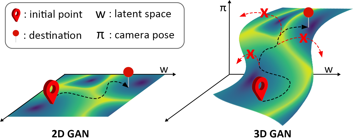
Figure 1: Comparison of the latent spaces of 2D GANs and 3D GANs. The explicit control of the camera parameter is the main property of 3D GANs that takes latent space into higher dimensions, making the inversion process harder. Finding both latent features at the same time is much more prone to fall into the local minima.

However, editing an image by projecting it onto the latent space of a 2D GAN makes the task vulnerable to the same set of problems of 2D GANs. As training methods of 2D GANs do not take into account the underlying geometry of an object, they offer limited control over the geometrical aspects of the generated image. Thus, manipulating image viewpoint using the latent space of 2D GANs always runs into the issue of multi-view inconsistency.

On the other hand, 3D-aware image synthesis addresses this issue by integrating explicit 3D representations into the generator architecture and enabling explicit control over the camera pose. With the success of neural radiance fields (NeRF) [34] in novel view synthesis, recent 3D-aware generation models employ a NeRF-based generator, which condition the neural representations on sample noise or disentangled appearance and shape codes in order to represent diverse 3D scenes or object. More recent attempts address the quality gap between 3D GANs and 2D GANs by adopting 2D CNN-based upsampler or efficient point sampling strategy, which enables the generation of high-resolution and photorealistic images on par with 2D GANs.

Projecting a 2D image onto the learned manifold of these 3D GANs unlocks many opportunities in computer vision applications. Not only can it generate multi-view consistent images from the acquired latent code, but it can also gather the exact surface geometry from the image. Furthermore, recent 3D GANs adopted a style-based generator module to learn the disentangled representations of 3D geometry and appearance. Similar to the latent-based image editing tasks of 2D GANs, by manipulating the latent code of a style-based 3D-aware generator, we can manipulate the semantic attributes of the reconstructed 3D model.

Despite its usefulness, few research have been conducted on 3D GAN inversion. Since 3D-aware GANs initially require a random vector and camera pose for their image generation, an inversion process to reacquire the latent code of a given image necessitates the camera pose of the image, information which real-life images usually often lack. Most of the existing methods require ground-truth camera information or must rely on the off-the-shelf geometry and camera pose from the 3D morphable model, which limit their application to a single category.

In this work, we propose a 3D-GAN inversion method that iteratively optimizes both the latent code and 3D camera pose of a given image simultaneously. We build upon the recently proposed 2D GAN inversion method that first inverts the given image into a pivot code, and then slightly tunes the generator based on the fixed pivot code (i.e. pivotal tuning [41]), which showed prominent results in both reconstruction and editability. Similarly, we acquire both the latent code and camera pose simultaneously as a pivot and fine-tune the pre-trained 3D-GAN to alter the generator manifold into pivots. Note that this is non-trivial since shape and camera direction compromise each other during optimization.

Recognizing the interdependency between latent code and camera parameter, we use a hybrid of learning and optimization-based approach by first using an encoder to infer a rough estimate of the camera pose and latent code, and further refining it to an optimal destination. As can be seen in our experiments, giving a good initial point for optimizing pivots much less falls into the local minimum. In order to further enforce the proximity of camera viewpoint, we introduce regularization loss that utilizes traditional depth-based image warping [55].

We demonstrate that our method enables high-quality reconstruction and editing while preserving multi-view consistency, and show that our results are applicable to a multitude of different categories. While we evaluate our proposed method on EG3D [7], the current state-of-the-art 3D-aware GAN, our method is also relevant to other 3D-aware GANs that leverage NeRF for its 3D representation.

2 Related Work

Generative 3D-Aware Image Synthesis.

3D-aware GANs aim to generate 3D-aware images from 2D image collections. The first approaches utilize voxel-based representation [35], which lacks fine details in image generation, due to memory inefficiency from its 3D representation. Starting from [43], several works achieved better quality by adopting NeRF-based representation, even though they struggle on generating high-resolution images due to the expensive computational cost of volumetric rendering. Some approaches proposed an efficient point sampling strategy [43, 11, 50], while others adopted 2D CNN-layers to efficiently upsample the volume rendered feature map [37, 16, 54]. Recently, other methods proposed hybrid representations to reduce computational burden from MLP layers, while achieving high-resolution image generation [7, 51, 44, 46]. Especially, our work is implemented on EG3D [7], which achieved state-of-the-art image quality while preserving 3D-consistency.

2D GAN Inversion.

The first step in applying latent-based image editing on real-world images is to project the image to the latent space of pre-trained GANs. Existing 2D GAN inversion approaches can be categorized into optimization-based, learning-based, and hybrid methods. Optimization approaches [1, 9] directly optimize the latent code for a single image. This method can achieve high reconstruction quality but is slow for inference. Unlike per-image optimization, learning-based approaches [40, 47, 3] use a learned encoder to project images. These methods have shorter inference time but fail to achieve high-fidelity reconstruction. Hybrid approaches are a proper mixture of the two aforementioned methods. [17, 58] used the cooperative learning strategy for encoder and direct optimization. PTI [41] fine-tunes StyleGAN parameters for each image after obtaining an initial latent code, solving the trade-off [47] between reconstruction and editability.

3D GANs Inversion.

3D GAN inversion approaches share the same goal as 2D GAN inversion with the additional need for the extrinsic camera parameters. Few existing methods solving inverse problems in 3D GANs propose effective training solutions of their own. [10] proposed regularization loss term to avoid generating unrealistic geometries by leveraging the popular CLIP [39] model. [29] can animate the single source image to resemble the target video frames, but is limited to human face as it requires off-the-shelf models [14] to extract expression, pose, and shape. [6] proposes a joint distillation strategy for training encoder, which is inadequate for 3D GANs that contain mapping function.

Image Manipulation.

Image manipulation can be conducted by changing the latent code derived from GAN inversion. Many works have examined semantic direction in the latent spaces of pre-trained GANs and then utilized it for editing. While some works [45, 2] use supervision in the form of semantic labels predicted by off-the-shelf attribute classifiers or annotated images, they are often limited to known attributes. Thus, other researchers resorted to using an unsupervised approach [18] or contrastive learning based methods [52, 38] to find meaningful directions. In this work, we leverage GANSpace [18], which performs principal component analysis in the latent space, to demonstrate latent-based manipulation of 3D shape.

3 Preliminaries

2D GANs Inversion and Pivotal Tuning.

Given a pretrained 2D generator $\mathcal{G}_{\mathrm{2D}}(\cdot\,;\theta)$ parameterized by weights $\theta$, 2D GANs inversion aims to find the latent representation $\mathbf{w}$ that can be passed to the generator to reconstruct a given image $x$:

$$\mathbf{w}^{*}=\underset{\mathbf{w}}{\mathrm{argmin}}\;\mathcal{L}(x,\mathcal{G}_{\mathrm{2D}}(\mathbf{w};\theta)),$$ (1)

where the loss function $\mathcal{L}(\cdot,\cdot)$ is usually defined as pixel-wise reconstruction loss or perceptual loss [53] between the given image $x$ and reconstructed image $\mathcal{G}_{\mathrm{2D}}(\mathbf{w};\theta)$.

To improve the performance, some other methods aim to optimize an encoder $\mathcal{E}(x;\theta_{\mathcal{E}})$ with parameters $\theta_{\mathcal{E}}$ that maps images to their latent representations such that:

$$\theta^{*}_{\mathcal{E}}=\underset{\theta_{\mathcal{E}}}{\mathrm{argmin}}\;\mathcal{L}(x,\mathcal{G}_{\mathrm{2D}}(\mathcal{E}(x;\theta_{\mathcal{E}});\theta)).$$ (2)

Some recent methods [58, 5, 57] take a hybrid approach of leveraging the encoded latent representation $\theta_{\mathcal{E}}(x;\theta_{\mathcal{E}})$ with learned parameters $\theta_{\mathcal{E}}$ as an initialization for a subsequent optimization process for (1), resulting in a faster and more accurate reconstruction.

Furthermore, it has been recently well studied that existing GANs inversion methods [47, 59, 2] struggle on the trade-offs between reconstruction and editability. To overcome this, [41] proposed a pivotal tuning stage in a manner that after finding the optimal latent representation $\mathbf{w}^{*}$, called the pivot code, the generator weights $\theta$ are fine-tuned so that the pivot code can more accurately reconstruct the given image while keeping its editability:

$$\theta^{*}=\underset{\theta}{\mathrm{argmin}}\;\mathcal{L}(x,\mathcal{G}_{\mathrm{2D}}(\mathbf{w}^{*};\theta)).$$ (3)

By utilizing the pivot code $\mathbf{w}^{*}$ and the tuned weights $\theta^{*}$, the final reconstruction is obtained as $y^{*}=\mathcal{G}_{\mathrm{2D}}(\mathbf{w}^{*};\theta^{*})$.

NeRF and 3D-aware GANs.

Neural Radiance Fields (NeRF) [34] achieves a novel view synthesis by employing a fully connected network to represent implicit radiance fields that maps location and direction $(\mathbf{x},\mathbf{d})$ to color and density $(\mathbf{c},\sigma)$. Specifically, along with each projected ray $r$ for a given pixel, $M$ points are sampled as $\{t_{i}\}^{M}_{i=1}$, and with the estimated color and density $(\mathbf{c}_{i},\sigma_{i})$ of each sampled point, the RGB value $c(r)$ for each ray can be calculated by volumetric rendering as:

$$c(r)=\sum_{i=1}^{M}T_{i}(1-\mathrm{exp}(-\sigma_{i}\delta_{i}))\mathbf{c}_{i},$$ (4)

where $T_{i}=\mathrm{exp}\left(-\sum_{j=1}^{i-1}\sigma_{j}\delta_{j}\right)$, and $\delta_{i}$ is the distance between adjacent sampled points such that $\delta_{i}=t_{i+1}-t_{i}$. Furthermore, per-ray depth $d(r)$ can also be approximated as

$$d(r)=\sum_{i=1}^{M}T_{i}(1-\mathrm{exp}(-\sigma_{i}\delta_{i}))t_{i}.$$ (5)

While NeRF trains a single MLP on multiple posed images of a single scene, NeRF-based generative models [16, 7] often condition the MLP on latent style code $\mathbf{w}$ that represents individual latent features learned from unposed image collections. These style-based 3D GANs have been popularly used in 3D aware image generation [16, 7, 54], and we denote this generator $\mathcal{G}_{\mathrm{3D}}(\mathbf{w},\pi;\theta)$ with a given latent code $\mathbf{w}$, which can be formally represented as the conditional function: $\{c,d\}=\mathcal{G}_{\mathrm{3D}}(\mathbf{w},\pi;\theta)$, where $c$ is rendered $\mathit{RGB}$ image and $d$ is depth map.

4 Method

4.1 Overview

Our objective, which we call 3D GAN inversion, is to project a real photo into the learned manifold of the GAN model. However, finding the exact match for $\mathbf{w}^{*}$ and $\pi^{*}$ for a given image $x$ is a non-trivial task since one struggles to optimize if the other is drastically inaccurate. To overcome this, we follow [58, 5, 57] to first construct two encoders that approximately estimate the initial codes from $x$ by $\mathbf{w}=\mathcal{E}(x;\theta_{\mathcal{E}})$ and $\pi=\mathcal{P}(x;\theta_{\mathcal{P}})$ (Sec. 4.2), and further solving optimization problem(Sec. 4.3). In particular, we introduce loss functions employed in (Sec. 4.3) and further discuss the effects and purposes of employing these loss functions(Sec. 4.4). An overview of our method is shown in Fig. 2.

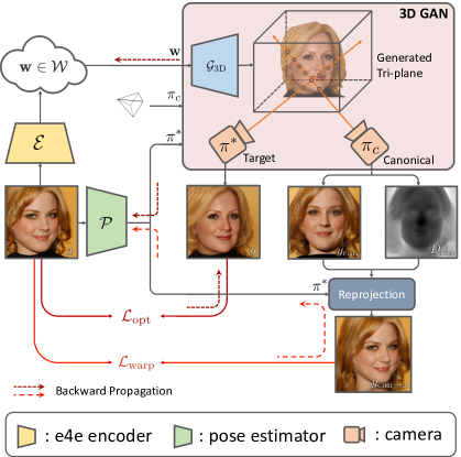
Figure 2: Overall architecture. This figure shows our method using depth-based warping to optimize latent code and camera pose simultaneously 4.3.

Input	Ours	SG2	SG2 $\mathcal{W}+$	PTI	SG2†	SG2† $\mathcal{W}+$	PTI†

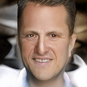
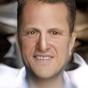
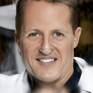
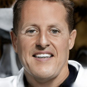
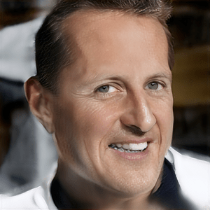
Figure 3: Comparison of novel view synthesis of out-of-domain samples. Given the optimized camera pose $\hat{\pi}$ and latent code $\hat{\mathbf{w}}$ obtained by each method, we explicitly control the viewpoint of the generated facial scene, by differing $\pi$ for different camera viewpoint. We compare our 3D GAN inversion method to standard 2D GAN inversion methods by applying the gradient-based optimization to both the latent code and the camera pose. We also leverage the same methods only on the latent code with the given ground-truth camera pose, and show the results labeled with ^†.

4.2 Latent Encoder $\mathcal{E}$ and Pose Estimator $\mathcal{P}$

For better 3D GANs inversion, utilizing a well-trained estimator for initialization should be considered [21, 48], but it is a solution limited to a single category. To obtain category-agnostic estimator, we first generate a pseudo dataset and its annotation pair $\{(\mathbf{w}_{\mathrm{ps}},\pi_{\mathrm{ps}}),x_{\mathrm{ps}}\}$ to pre-train our encoders, where $x_{\mathrm{ps}}=\mathcal{G}_{\mathrm{3D}}(\mathbf{w}_{\mathrm{ps}},\pi_{\mathrm{ps}};\theta)$. Thanks to the generation power of 3D-aware GANs, we can generate nearly unlimited numbers of pairs within the generator’s manifold. More specifically, for given latent encoder $\mathcal{E}$, let $\bigtriangleup\mathbf{w}=\mathcal{E}(x_{\mathrm{ps}};\theta_{\mathcal{E}})$ denote the output of the encoder, where $\mathbf{w}\in\mathbb{R}^{1\times 512}$. Following the training strategy of [47], we employ the generator $\mathcal{G}_{\mathrm{3D}}$ and its paired discriminator $\mathcal{D}$ to guide encoder to find the best replication of $x_{\mathrm{ps}}$ with $\bar{\mathbf{w}}+\bigtriangleup\mathbf{w}$, where $\bar{\mathbf{w}}$ is an average embeddings of $\mathcal{G}_{\mathrm{3D}}$. We provide more detailed implementation procedure of pre-training each network in the Appendix.

4.3 Optimization

After the pre-traininig step, given an image $x$, the learnable latent vector and camera pose are first initialized from trained estimators as $\mathbf{w}_{\mathrm{init}}=\bar{\mathbf{w}}+\mathcal{E}(x;\theta_{\mathcal{E}})$ and $\pi_{\mathrm{init}}=\mathcal{P}(x;\theta_{\mathcal{P}})$. Subsequently, they are further refined for a more accurate reconstruction. In this stage, we reformulate optimization step in (1) into the 3D GAN inversion task, in order to optimize the latent code and camera viewpoint starting from each initialization $\{\mathbf{w}_{\mathrm{init}},\pi_{\mathrm{init}}\}$, such that:

$$\mathbf{w}^{*},\pi^{*},n^{*}=\underset{\mathbf{w},\pi,n}{\mathrm{argmin}}\;\mathcal{L}^{\mathrm{opt}}(x,\mathcal{G}_{\mathrm{3D}}(\mathbf{w},\pi,n;\theta)),$$ (6)

where $n$ denotes the per-layer noise inputs of the generator and $\mathcal{L}^{\mathrm{opt}}$ contains employed loss functions on the optimization step. Note that, following the latent code optimization method in [41], we use the native latent space $\mathcal{W}$ which provides the best editability.

In addition, in the pivotal-tuning step, using the optimized latent code $\mathbf{w}^{*}$ and optimized camera pose $\pi^{*}$, we augment the generator’s manifold to include the image by slightly tuning $\mathcal{G}_{\mathrm{3D}}$ with following reformulation of (3):

$$\theta^{*}=\underset{\theta}{\mathrm{argmin}}\;\mathcal{L}^{\mathrm{pt}}(x,\mathcal{G}_{\mathrm{3D}}(\mathbf{w}^{*},\pi^{*},n^{*};\theta)).$$ (7)

In this optimization, following [41], we unfreeze the generator and tune it to reconstruct the input image $x$ with given $\mathbf{w}^{*}$ and $\pi^{*}$, which are both constant. We also implement the same locality regularization in [41]. Again, $\mathcal{L}^{\mathrm{pt}}$ denotes a combination of loss functions on the pivotal-tuning step.

4.4 Loss functions

LPIPS and MSE Loss.

To reconstruct the given image $x$, we adopt commonly used LPIPS loss for both optimization and pivotal tuning step. As stated in (6), the loss is used to train the both latent code $\mathbf{w}$ and camera pose $\pi$. Additional mean square error is given only at the pivotal tuning step, which is commonly used to regularize the sensitivity of LPIPS to adversarial examples. Formally, our losses can be defined by:

$$\mathcal{L}_{\mathrm{lpips}}=\mathcal{L}_{\mathrm{lpips}}(x,\mathcal{G}^{\mathrm{c}}_{\mathrm{3D}}(\mathbf{w},\pi,n;\theta)),$$ (8)

$$\mathcal{L}_{L2}=\mathcal{L}_{L2}(x,\mathcal{G}^{\mathrm{c}}_{\mathrm{3D}}(\mathbf{w},\pi,n;\theta)).$$ (9)

Depth-based Warping Loss.

Similar to [55], every point on the target image can be warped into other viewpoints. We consider the shape representation of $\mathbf{w}$ latent code plausible enough to fit in the target image. Given a canonical viewpoint $\pi_{\mathrm{can}}$, we generate a pair of image and depth map $\{y_{\mathrm{can}},D_{\mathrm{can}}\}=\mathcal{G}_{\mathrm{3D}}(\mathbf{w},\pi_{\mathrm{can}};\theta)$. Let $y_{\mathrm{can}}(r)$ denote the homogeneous coordinates of a pixel $\gamma$ in the generated image of a canonical view $\pi_{\mathrm{can}}$ using (4). Also for each $y_{\mathrm{can}}(r)$ we obtain the depth value $D_{\mathrm{can}}(r)$ by using (5).

Then we can obtain $y_{\mathrm{can}}(r)$’s projected coordinates onto the source view $\pi_{x}$ denoted as $\hat{y}_{x}(r)$ by

$$\hat{y}_{x}(r)\sim K\hat{\pi}_{\mathrm{can}\rightarrow x}D_{\mathrm{can}}(r)K^{-1}y_{\mathrm{can}}(r),$$ (10)

where K is the camera intrinsic matrix, and $\hat{\pi}_{\mathrm{can}\rightarrow x}$ is the predicted relative camera pose from canonical to source. As $\hat{x}(r)$ for every pixel $r$ are continuous values, following [55], we exploit the differentiable bilinear sampling mechanism proposed in [23] to obtain the projected 2D coordinates.

For simplicity of notation, from a generated image $y_{\mathrm{can}}=\mathcal{G}^{\mathrm{c}}_{\mathrm{3D}}(\mathbf{w},\pi_{\mathrm{can}};\theta)$, we denote the projected image as $y_{\mathrm{can}\rightarrow x}=y_{\mathrm{can}}\langle proj(D_{\mathrm{can}},\pi_{\mathrm{can}\rightarrow x},K)\rangle$, where $proj(\cdot)$ is the resulting 2D image using the depth map $D_{\mathrm{can}}$ and $\langle\cdot\rangle$ denotes the bilinear sampling operator, and define the objective function to calculate $\pi_{\mathrm{can}\rightarrow x}$:

$$\mathcal{L}_{\mathrm{warp}}=\mathcal{L}_{\mathrm{lpips}}\left(x,y_{\mathrm{can}}\langle proj(D_{\mathrm{can}},\pi,K)\rangle\right),$$ (11)

again using a LPIPS loss to compare the two images.

Depth Regularization Loss.

Neural radiance field is infamous for its poor performance when only one input view is available. Although tuning the parameters of 2D GANs seem to retain its latent editing capabilities, we found the NeRF parameters to be much more delicate, and tuning them to a single view degrades the 3D structure before reaching the desired expressiveness, resulting in low-quality renderings at novel views.

To mitigate this problem, we take advantage of the geometry regularization used in [36] and encourage the generated depth to be smooth, even from unobserved viewpoints. The regularization is based on the real-world observation that real geometry or depth tends to be smooth, and is more likely to be flat, and formulated such that depth for each pixel should not be too different from those of neighboring pixels. We enforce the smoothness of the generated depth $D(r)$ for each pixel $r$ with the depth regularization loss:

$$\begin{split}\mathcal{L}_{DR}(D)=\sum_{i,j=1}^{H-1,W-1}\left(\left(D(r_{i,j})-D(r_{i+1,j})\right)^{2}\right.\\ +\left.(\left(D(r_{i,j})-D(r_{i,j+1})\right)^{2}\right),\end{split}$$ (12)

where $H$ and $W$ are the height and width of the generated depth map, and $r_{i,j}$ indicates the ray through pixel (i, j). Note that while [36] implements the geometry regularization by comparing overlapping patches, we utilize the full generated depth map $D$ for our implementation.

Overall Loss Function.

Ultimately, we define the entire optimization step with a generated image and depth $\{y,D\}=\mathcal{G}_{\mathrm{3D}}(\mathbf{w},\pi,n;\theta)$:

$$\begin{split}\mathcal{L}^{\mathrm{opt}}=&\;\,\mathcal{L}_{\mathrm{lpips}}(x,y)\\ &+\lambda_{\mathrm{warp}}\mathcal{L}_{\mathrm{warp}}(x,y_{\mathrm{can}},D)+\lambda_{n}\mathcal{L}_{n}(n),\end{split}$$ (13)

and the pivotal tuning process is defined by:

$$\begin{split}\mathcal{L}^{\mathrm{pt}}=&\;\,\mathcal{L}_{\mathrm{lpips}}(x,y)\\ &+\lambda_{L2}\mathcal{L}_{L2}(x,y)+\lambda_{DR}\mathcal{L}_{DR}(D),\end{split}$$ (14)

where $\mathcal{L}_{n}$ denotes the noise regularization loss proposed in [27], which prevents the noise from containing crucial signals of the target image.

5 Experimental Results

5.1 Experimental Settings

Input	Ours	SG2	SG2 $\mathcal{W}+$	PTI	SG2†	SG2† $\mathcal{W}+$	PTI†

Figure 4: 2D and 3D Reconstruction of out-of-domain samples. We compare both the image reconstruction and 3D reconstruction capabilities of each method, where the 3D shapes are iso-surfaces extracted from the density field using marching cubes. Methods labeled with $\dagger$ use ground-truth camera pose.

Datasets.

We conduct the experiments on two 3D object types, human faces and cat faces, as they are the two most popular tasks in GAN inversion. For all experiments, we employ the pre-trained EG3D [7] generator. For human faces, we use the weights pre-trained on the cropped FFHQ dataset [25], and we evaluate our method with the CelebA-HQ validation dataset [24, 32]. We also use the pre-trained weights on the AFHQ dataset [8] for cat faces and evaluate on the AnimalFace10 dataset [31].

Baselines.

Since the current works [10, 29] do not provide public source code for reproduction and comparison of their work, we mainly compare our methods with the popular 2D GAN inversion methods: The direct optimization scheme proposed by [27] to invert real images to $\mathcal{W}$ denoted as SG2, a similar method but extended to $\mathcal{W}+$ space [1] denoted as SG2 $\mathcal{W}+$, and the PTI method from [41]. We adopt these methods to work with the pose-requiring 3D-aware GANs, either by providing the ground-truth camera pose during optimization or using the same gradient descent optimization method for the camera pose.

Method	MSE$\downarrow$	LPIPS$\downarrow$	MS-SSIM$\uparrow$	ID Sim.$\uparrow$	FID $\downarrow$
SG2	0.0277	0.3109	0.5889	0.0957	36.0291
SG2 $\mathcal{W}+$	0.0163	0.2398	0.6833	0.2906	32.3971
PTI	0.0036	0.0789	0.8221	0.6671	32.7366
SG2†	0.0232	0.2898	0.6151	0.1125	34.7612
SG2† $\mathcal{W}+$	0.0117	0.2029	0.7349	0.3972	31.1732
PTI†	0.0033	0.0722	0.8309	0.6737	28.5911
Ours	0.0035	0.0777	0.8280	0.7013	30.1192

Table 1: Qualitative reconstruction results measured over the CelebA-HQ test set using various similarity metrics. We also measure the quality of random views of the reconstructed face. The best and runner-up values are marked bold and underlined, respectively. Methods labeled with $\dagger$ use ground-truth camera pose.

Input

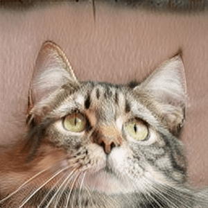
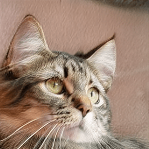
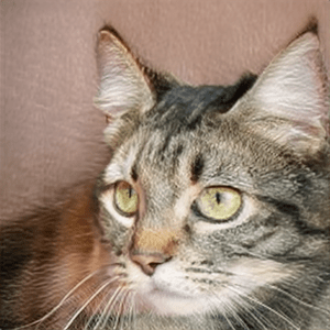
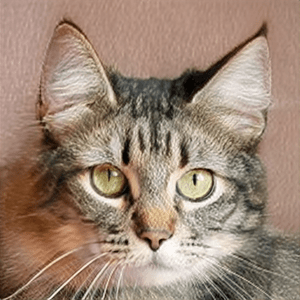
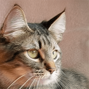
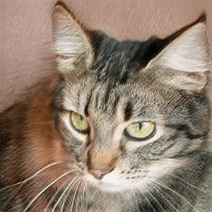
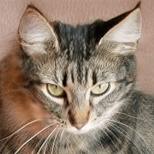
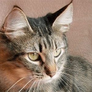
Figure 5: Reconstruction and novel view synthesis on AnimalFace10 dataset. Our inversion method is not limited to the facial domain and can be applied to other datasets.

	Input	Ours	SG2	SG2 $\mathcal{W}+$	PTI	SG2†	SG2† $\mathcal{W}+$	PTI†
$-$Age
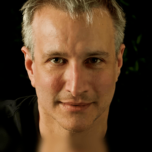
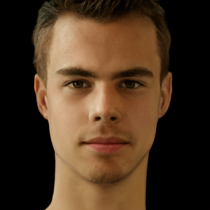
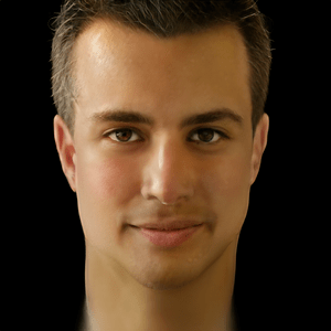
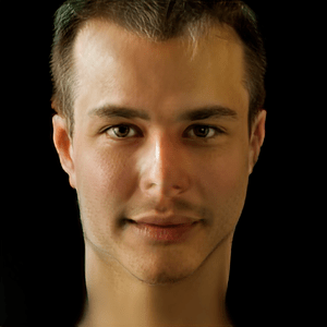
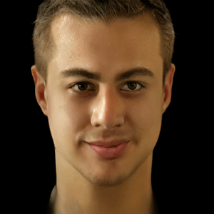
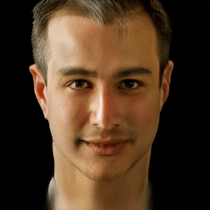
$+$Smile

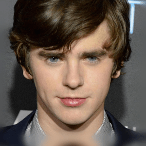
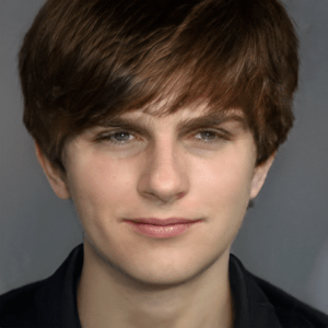
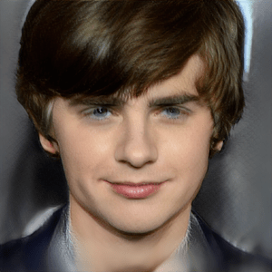
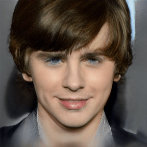
Figure 6: Editing Quality Comparison We perform various edits [18] over latent codes and camera pose acquired by each method. Benefiting from the capabilities of 3D-aware GANs, we also compare edited 3D shape generated from the edited latent codes. Our method achieves both realistic and accurate manipulation and is also more capable of preserving the identity and geometry of the original input. Methods labeled with $\dagger$ use ground-truth camera pose.

5.2 Reconstruction

Quantitative Evaluation.

For quantitative evaluation, we reconstruct 2,000 validation images of CelebA-HQ and utilize the same standard metrics used in 2D GAN inversion literature: pixelwise L2 distance using MSE, perceptual similarity metric using LPIPS [53] and structural similarity metric using MS-SSIM [49]. In addition, for facial reconstruction, we follow recent 2D GAN inversion works [13, 4] and measure identity similarity using a pre-trained facial recognition network of CurricularFace [22]. Furthermore, we also need to measure the 3D reconstruction ability of our method, as the clear advantage of 3D GAN inversion over 2D GAN inversion is that the former allows for novel view synthesis given a single input image. In other words, the latent code acquired by a successful inversion process should be able to produce realistic and plausible images at random views. In order to measure image quality, we calculate the Frechet Inception Distance (FID) [20] between the original images and 2,000 additionally generated images from randomly sampled viewpoints.

The results are shown in Table 1. As can be seen, compared to the 2D GAN inversion methods that use the same gradient-based optimization for camera pose, using the depth-based warping method better guides the camera viewpoint to the desired angle, showing higher reconstruction metrics. Furthermore, while methods designed for high expressiveness such as SG2 $\mathcal{W}+$ and PTI achieve comparable pixel-wise reconstruction abilities, our method has the upper hand when it comes to 3D reconstruction, producing better quality images for novel views of the same face. Even compared to inversion methods using ground-truth camera pose, our method achieves competitive results without external data and reliably predicts the camera pose, showing similar reconstruction scores for each metric.

Qualitative Evaluation.

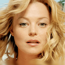
	2D
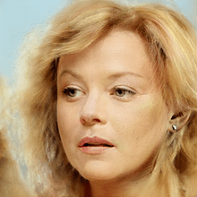
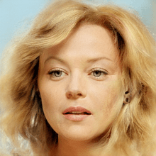
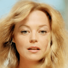
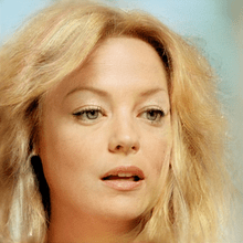
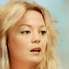
	3D
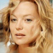
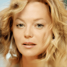
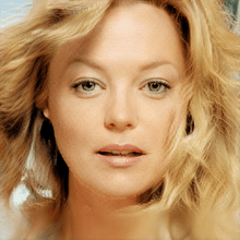
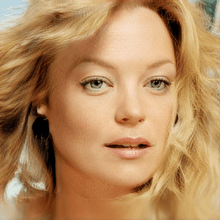
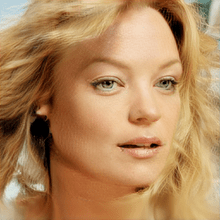
	2D
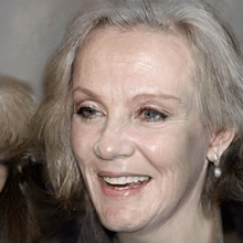
	3D

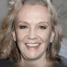
Figure 4: Comparison of pose manipulation of real images inverted with 2D GANs and 3D GANs. As can be seen, pose manipulation using PTI on StyleGAN2 (first row) only allows for implicit control by the editing magnitude and larger step sizes result in undesired transformations. On the other hand, using our method on EG3D (second row), allows for explicit control and because the acquired latent representation are viewpoint independent, the edits geometrically consistent.

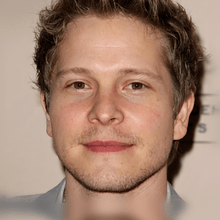
+ Age		2D
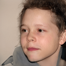
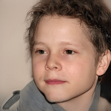
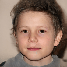
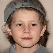
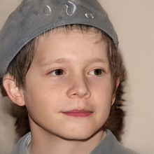
		3D
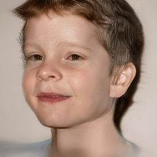
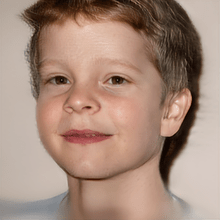
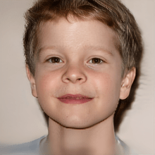
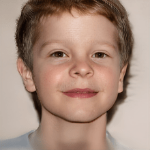
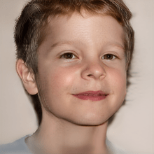
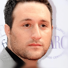
+ gender		2D
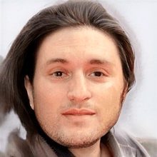
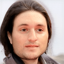
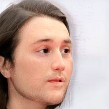
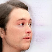
		3D

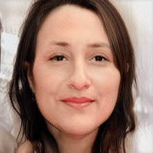
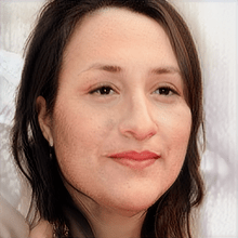
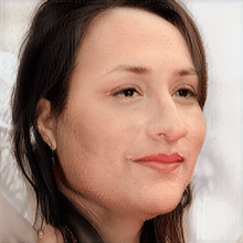
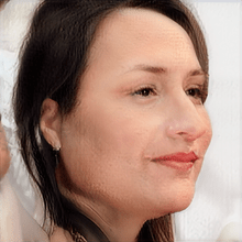
Figure 5: Additional results of simultaneous attribute editing and viewpoint shift comparison of 2D and 3D GANs. We compare editing results of applying attribute editing (smile) and viewpoint interpolation at the same time on the latent code acquired by PTI [41] on StyleGAN2 [27] and the latent code acquired by our method on EG3D [7]

We first visualize the reconstruction results in Fig. 3, which illustrates reconstruction and novel views rendered with our method and the baseline. Notably, our method achieves comparable results to methods using ground-truth pose, while showing much better reconstruction compared to gradient-based camera estimation. Not only do we provide qualitative comparison of the visual quality of inverted images, but we also show reconstructed 3D shape of the given image as a mesh using the Marching Cubes algorithm [33], as demonstrated in Fig. 4. Different from 2D GAN inversion, we also compare the 3D geometry quality of each face by comparing the rendered views of different camera poses. Furthermore, we evaluate reconstruction and novel view synthesis on cat faces in Fig. 5

While SG2 $\mathcal{W}+$ and PTI show reasonable reconstruction result at the same viewpoint, when we steer the 3D model to different viewpoints, the renderings are incomplete and show visual artifacts with degraded 3D consistency. In contrast, we can see that by using our method, we can synthesize novel views with comparable quality to methods requiring ground-truth viewpoints.

5.3 Editing Quality

We employ GANSpace [18] method to quantitatively evaluate the manipulation capability of the acquired latent code. In Fig. 6, we compare latent-based editing results to the 2D GAN-inversion methods used directly to 3D-aware GANs. Consistent with 2D GANs, the latent code found in the $\mathcal{W}+$ space produces more accurate reconstruction but fails to perform significant edits, while latent codes in $\mathcal{W}$ space show subpar reconstruction capability. Using pivotal tuning [41] preserves the identity while maintaining the manipulation ability of $\mathcal{W}$ space. Reinforcing [41] with our more reliable pose estimation and regularized geometry, our method best preserves the 3D-aware identity while successfully performing meaningful edits. We also provide quantitative evaluation in the supplementary material.

5.4 Comparison with 2D GANs

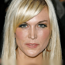
	2D
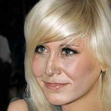
	3D

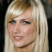
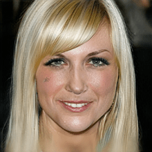
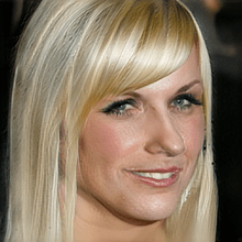
Figure 7: Simultaneous attribute editing and viewpoint shift comparison of 2D and 3D GANs. We compare editing results of applying attribute editing (smile) and viewpoint interpolation at the same time on the latent code acquired by PTI [41] on StyleGAN2 [27] and the latent code acquired by our method on EG3D [7]

$\mathcal{E}\&\mathcal{P}$	$\mathcal{L}_{\mathrm{warp}}$	$\mathcal{L}_{DR}$	LPIPS$\downarrow$	MS-SSIM$\uparrow$	ID Sim.$\uparrow$	FID$\downarrow$
✗	✗	✗	0.0789	0.8221	0.6671	32.7366
✓	✗	✗	0.0780	0.8259	0.6823	31.1518
✗	✓	✗	0.0783	0.8248	0.6750	31.3179
✓	✓	✗	0.0771	0.8295	0.7005	30.6272
✓	✓	✓	0.0777	0.8280	0.7013	30.1198

Table 2: Reconstruction metric comparison of various combinations of proposed methods. We evaluate our proposed optimization scheme by experimenting with certain combinations of proposed methods. We mark (✓) when the given method is employed and (✗) when it is not.

We demonstrate the effectiveness and significance of 3D-aware GAN inversion by comparing the viewpoint manipulation using the explicit camera pose control for EG3D and latent space. Even though [28] points out that 3D GANs lack the ability to manipulate semantic attributes, recent advancements of NeRF-based generative architectures have achieved a similar level of expressiveness and editability to 2D GANs. As recent 3D-aware GANs such as EG3D can generate high-fidelity images with controllable semantic attributes while maintaining a reliable geometry, image editing using 3D GANs offers consistent multi-view results which are more useful.

In Fig. 7, we compare the simultaneous manipulation abilities of 2D and 3D-aware GANs. While pose manipulation of 2D GANs only allows for implicit control by the editing magnitude, 3D-aware GANs enable explicit control of the viewpoint. Also, the edited images in 2D GANs are not view consistent and large editing factors result in undesired transformations of the identity and editing quality. In contrast, pose manipulation of 3D GANs is always multi-view consistent, thus produces consistent pose interpolation even for an edited scene.

5.5 Ablation Study

In Table 2 we show the importance of the various components of our approach by turning them on and off in turn. To further investigate the efficacy of our methodology, we further show some visual results for more intuitive comparisons.

Importance of initialization.

We test the effectiveness of our design by comparing our full hybrid method to the single-encoder methods and show the results in Fig. 8 and Table 3. We show that using a hybrid approach consisting of learned encoder $\mathcal{E}$ and gradient-based optimization is the ideal approach when obtaining the latent code. Similarly, leveraging a pose estimator $\mathcal{P}$ for initialization for the pose refinement also shortens the optimization time.

		0 iter	150 iter	300 iter		tuned
Input	$\mathcal{E}$				…
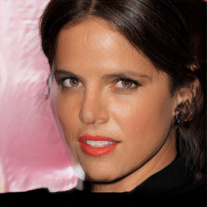
	$\mathcal{P}$				…
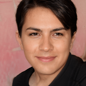
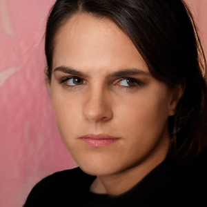
	$\mathcal{E}$ & $\mathcal{P}$				…

Figure 8: Importance of initialization We selectively employ the latent encoder $\mathcal{E}$ and pose estimator $\mathcal{P}$ and compare their optimization process.

$\mathcal{E}$	$\mathcal{P}$	MSE$\downarrow$	LPIPS$\downarrow$	MS-SSIM$\uparrow$	ID Sim.$\uparrow$	$\theta$	$\phi$
✗	✓	0.0036	0.0782	0.8263	0.6958	3.19	2.90
✓	✗	0.0038	0.0790	0.8219	0.6810	5.73	5.93
✓	✓	0.0035	0.0777	0.8280	0.7013	3.16	2.70

Table 3: Importance of initialization. We state the importance of utilizing pre-trained latent encoder $\mathcal{E}$ and pose estimator $\mathcal{P}$ as an initialization for optimization, by comparing the optimization results that started from network outputs(✓) and those that started from random initialization(✗).

Effectiveness of Geometry Regularization.

We study the role of depth smoothness regularization in the pivotal tuning step by varying the weight $\lambda_{DR}$. We show the generated geometry and its pixelwise MSE value after fine-tuning the generator in Fig. 9. While solely using the reconstruction loss leads to better quantitative results, novel views still contain floating artifacts and the generated geometry has holes and cracks. In contrast, including the depth smoothness regularization with its weight as $\lambda_{DR}=1$ enforces solid and smooth surfaces while producing accurate scene geometry. It should be noted that a high weight for the depth smoothness blurs the fine segments of the generated geometry such as hair.

Input	$\lambda_{DR}=0$	$\lambda_{DR}=1$	$\lambda_{DR}=50$
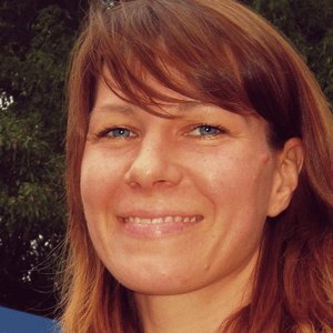
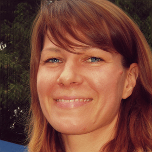
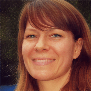
	L2: 0.1233	L2: 0.1255	L2: 0.1257

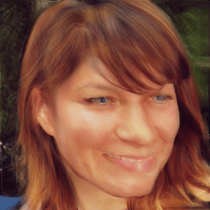
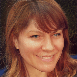
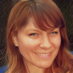
Figure 9: Comparison of different weights of depth smoothness loss during the pivotal tuning stage. Although excluding depth smoothness shows the best reconstruction result (first row), the reconstructed geometry is distorted (third row) and provides malformed renderings for novel views (second row). Best viewed in zoom.

6 Conclusion

We present a geometric approach for inferring both the latent representation and camera pose of 3D GANs for a single given image. Our method can be widely applied to the 3D-aware generator, by utilizing hybrid optimization method with additional encoders trained by manually built pseudo datasets. In essence, this pre-training session helps the encoder acquire the representation power and geometry awareness of 3D GANs, thus finding a stable optimization pathway. Moreover, we utilize several loss functions and demonstrate significantly improved results in reconstruction and image fidelity both quantitatively and qualitatively. It should be noted that whereas previous methods used 2D GANs for editing, our work suggests the possibility of employing 3D GANs as an editing tool. We hope that our approach will encourage further research on 3D GAN inversion, which will be further utilized with the single view 3D reconstruction and semantic attribute editings.

Appendix A Implementation Details

A.1 Architectures and Hyperparameters

To implement the latent code encoder $\mathcal{E}$, we follow both the implementation and training strategy of e4e [47], which is a well-proven encoder architecture to map the input image into the distribution of $\mathcal{W}+$. We manipulate the output dimension of the encoder into $\mathbb{R}^{1\times 512}$ to fit in our method. For the camera pose estimator $\mathcal{P}$, we manipulate the simple resnet34 [19] encoder to find theta and phi angles which are further calculated into the extrinsic matrix. In the case of dataset which has an additional roll angle component in the rotation such as cat faces, we choose the 6D rotation representation proposed by [56]. Although the target images are cropped and refined by [12], there exists an additional camera translation that euler angles cannot thoroughly define. Thus, we set an additional coordinate variance on the camera position as a learnable parameter. See supplementary for details and qualitative evaluation of additional translation.

A.2 Pre-training Latent Encoder $\mathcal{E}$ and Pose Estimator $\mathcal{P}$

In order to train the encoder $\mathcal{E}$, we adopt LPIPS loss [53] denoted as $\mathcal{L}^{\mathcal{E}}_{\mathrm{lpips}}$ in order to reconstruct the given image. Additionally, we minimize the gap between $\bar{\mathbf{w}}+\bigtriangleup\mathbf{w}$ and the embedding space $\mathcal{W}$ of $\mathcal{G}_{\mathrm{3D}}$ by employing non-saturating GAN loss [15] and delta-regularization loss:

$$\mathcal{L}^{\mathcal{E}}_{\mathrm{adv}}=-\mathbb{E}[\mathrm{log}\mathcal{D}(\mathcal{G}^{\mathrm{c}}_{\mathrm{3D}}((\bar{\mathbf{w}}+\bigtriangleup\mathbf{w}),\pi_{\mathrm{ps}};\theta))],$$ (1)

$$\mathcal{L}^{\mathcal{E}}_{\mathrm{reg}}=||\bigtriangleup\mathbf{w}||^{2}_{2}.$$ (2)

Moreover, in the case of pose estimator $\mathcal{P}$, the predicted output $\hat{\pi}$ from a given image is directly compared with $\pi_{\mathrm{ps}}$. Let rotation $\hat{\mathrm{R}}\in\mathbb{R}^{3\times 3}$, translation $\hat{t}\in\mathbb{R}^{3}$, and scale factor $\hat{s}\in\mathbb{R}^{1}$ denote as a decomposed set of $\pi$. Since the scale factor is given as a constant, we formulate our loss function as:

$$\mathcal{L}^{\mathcal{P}}_{\mathrm{rot}}=||\mathrm{R}^{-1}_{\mathrm{ps}}\cdot\hat{\mathrm{R}}-\mathrm{I}_{3\times 3}||_{2},$$ (3)

$$\mathcal{L}^{\mathcal{P}}_{\mathrm{trans}}=||t_{\mathrm{ps}}-\hat{t}||_{2},$$ (4)

where $\mathrm{R}_{\mathrm{ps}}$ and $t_{\mathrm{ps}}$ are decomposition of $\pi_{\mathrm{ps}}$, and $\mathrm{I}_{3\times 3}$ is identity matrix.

In summary, our total loss functions ($\mathcal{L}^{\mathcal{E}}$ for Latent Encoder $\mathcal{E}$ and $\mathcal{L}^{\mathcal{P}}$ for Pose Estimator $\mathcal{E}$) for pre-training the encoder are defined by:

$$\mathcal{L}^{\mathcal{E}}=\mathcal{L}^{\mathcal{E}}_{\mathrm{lpips}}+\lambda_{\mathrm{adv}}\mathcal{L}^{\mathcal{E}}_{\mathrm{adv}}+\lambda_{\mathrm{reg}}\mathcal{L}^{\mathcal{E}}_{\mathrm{reg}},$$ (5)

$$\mathcal{L}^{\mathcal{P}}=\mathcal{L}^{\mathcal{P}}_{\mathrm{rot}}+\lambda_{\mathrm{trans}}\mathcal{L}^{\mathcal{P}}_{\mathrm{trans}}.$$ (6)

A.3 Pseudo Dataset

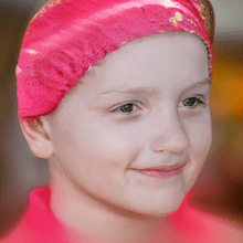
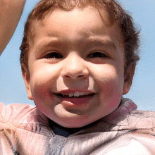
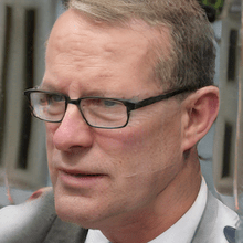
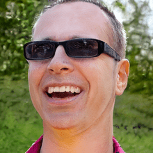
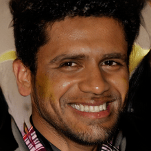
Figure 1: Generated pseudo ground-truth images for training latent encoder and pose estimator. We utilize EG3D as a pseudo ground-truth generator to sample images paired with corresponding latent representations and camera viewpoint. These pseudo pairs $\{\mathbf{w},I_{\mathrm{pseudo}}\}$ and $\{\mathbf{\pi},I_{\mathrm{pseudo}}\}$ are used as training data for latent encoder and pose estimator respectively.

We visualize a randomly selected pseudo dataset in Fig. 1. We construct 30,000 number of pseudo pairs for human faces, and 10,000 for cat faces. Each of the pseudo pairs rendered from a unique latent vector $\mathbf{w}_{\mathrm{ps}}$ with randomly sampled camera pose parameter $\pi_{\mathrm{ps}}$ within the camera pose boundary given by [7]. As can be seen from Fig. 1, the generative power of 3D GANs gives promising guidance both for the latent encoder and pose estimator. In the case of cat faces, we additionally gave a roll rotation to the pose parameter which gives the generated pseudo images to rotate on the image plane.

A.4 Preparing Facial Images for GAN Inversion.

EG3D [7] uses a slightly different cropping method for their training process. We follow the official code, found here: https://github.com/NVlabs/eg3d/tree/FFHQ_preprocess which uses face detection and pose-extraction pipeline [12] in order to identify and crop the face region and infer the camera viewpoint of the image. The inferred camera viewpoint is leveraged in our baseline 2D GAN inversion implementation and is also exploited as a ground-truth dataset to evaluate our pose estimation performance.

A.5 Implementation Details of Comparison Baselines.

The following algorithms show our method, along with comparisons using 2D GAN inversion methods directly to 3D-aware GANs.

Input: real image $x$; canonical pose $\pi_{c}$; gradient-based optimizer $F^{\prime}$; depth smoothness regularizer $DR$; depth based reprojection $proj(\cdot)$; camera intrinsics $K$

Output: the reconstructed image $\hat{y}$

1 Initialize() the code and pose $(w,\pi)$ = $(w^{\prime},\pi^{\prime})$;

2 while not converged do

3       $Loss\leftarrow L\left(x,\mathcal{G}^{\mathrm{c}}_{\mathrm{3D}}(\mathbf{w},\pi;\theta)\right)$;

4       $w\leftarrow w-\eta F^{\prime}(\nabla_{w}Loss)$;

5       $\mathrm{projected}\leftarrow\mathcal{G}^{\mathrm{c}}_{\mathrm{3D}}(\mathbf{w},\pi;\theta)\langle proj(\mathcal{G}^{\mathrm{d}}_{\mathrm{3D}}(\mathbf{w},\pi;\theta),\pi,K)\rangle$ ;

6       $Loss\leftarrow L\left(\mathcal{G}^{\mathrm{c}}_{\mathrm{3D}}(\mathbf{w},\pi;\theta)),\mathrm{projected},\right)$;

7       $\pi\leftarrow\pi-\eta F^{\prime}(\nabla_{\pi}Loss)$;

8      

9 end while

10while not converged do

11       $Loss\leftarrow L\left(x,\mathcal{G}^{\mathrm{c}}_{\mathrm{3D}}(\mathbf{w},\pi;\theta))\right)+DR(\mathcal{G}^{\mathrm{d}}_{\mathrm{3D}}(\mathbf{w},\pi;\theta))$;

12       $\theta\leftarrow\theta-\eta F^{\prime}(\nabla_{\theta}Loss)$;

13      

14 end while

$\hat{y}\leftarrow\mathcal{G}^{\mathrm{c}}_{\mathrm{3D}}(\mathbf{w},\pi;\theta)$

Algorithm 1 Our proposed method.

Input: real image $x$ from viewpoint $\pi^{*}$; a pre-trained generator $\mathcal{R}(\cdot,G(\cdot;\theta))$; gradient-based optimizer $F^{\prime}$.

Output: the latent code $w$

1 Initialize() the code $w$ = $w^{\prime}$;

2 while not converged do

3       $Loss\leftarrow L\left(x,\mathcal{G}^{\mathrm{c}}_{\mathrm{3D}}(\mathbf{w},\pi^{*};\theta)\right)$;

4       $w\leftarrow w-\eta F^{\prime}(\nabla_{w}L)$;

5      

6 end while

7if pivotal tuning then

8       while not converged do

9             $Loss\leftarrow L\left(x,\mathcal{G}^{\mathrm{c}}_{\mathrm{3D}}(\mathbf{w},\pi^{*};\theta)\right)$;

10             $\theta\leftarrow\theta-\eta F^{\prime}(\nabla_{\theta}L)$;

11            

12       end while

13      

14 end if

Algorithm 2 GT camera pose during optimization.

Input: real image $x$; a pre-trained generator $\mathcal{R}(\cdot,G(\cdot;\theta))$; gradient-based optimizer $F^{\prime}$.

Output: the latent code $w$

1 Initialize() the code and pose $(w,\pi)$ = $(w^{\prime},\pi^{\prime})$;

2 while not converged do

3       $Loss\leftarrow L\left(x,\mathcal{G}^{\mathrm{c}}_{\mathrm{3D}}(\mathbf{w},\pi;\theta)\right)$;

4       $(w,\pi)\leftarrow(w,\pi)-\eta F^{\prime}(\nabla_{w,\pi}L)$;

5      

6 end while

7if pivotal tuning then

8       while not converged do

9             $Loss\leftarrow L\left(x,\mathcal{G}^{\mathrm{c}}_{\mathrm{3D}}(\mathbf{w},\pi;\theta)\right)$;

10             $\theta\leftarrow\theta-\eta F^{\prime}(\nabla_{\theta}L)$;

11            

12       end while

13      

14 end if

Algorithm 3 Gradient descent to optimize camera.

Appendix B Discussion

B.1 Difficulties of 3D GAN inversion

As demonstrated in the main paper, 3D GAN inversion is non-trivial, since one struggles to optimize if the other is inaccurate. Optimizing latent features in 3D GANs gives an additional consideration to pose optimization, which needs to be optimized simultaneously. Specifically, this becomes difficult when either latent feature or camera pose is imperfect. In Fig. 2, we show failure cases to illustrate how the imperfect camera pose estimation leads to shape distortion. The second column of Fig. 2 is the final inversion result without pivotal tuning. As the pose estimation fails, the second column shows misalignment in the head pose. Even though the pivotal tuning step resolves the visual perception error, they often fail on novel view synthesis (4-6 columns). This is because the tuning procedure forces the implicit volume to fit into an input image with a misaligned camera parameter, which becomes distortions to the other viewpoints.

Input	Inv.	Pivotal Tuning		Novel Views		Mesh

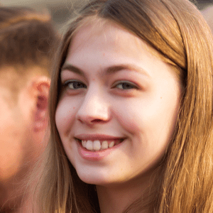
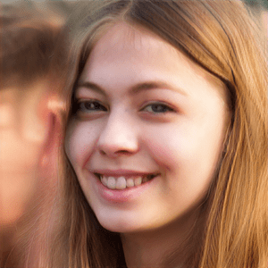
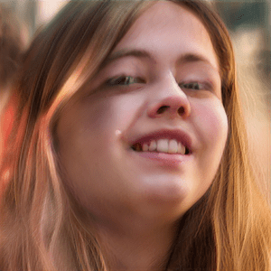
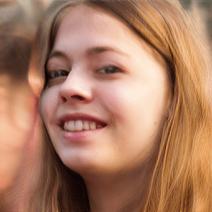
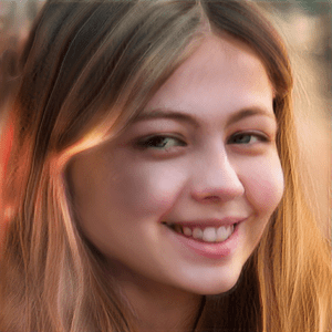
Figure 2: Importance of accurate camera pose estimation.

Furthermore, we conduct another ablation study on camera misalignment, illustrated in Fig. 3. The top row shows an inversion process using our training strategy, while the bottom row does not optimize the additional trainable translation vector. Following the preprocessing stage of [12], they create a by-product of camera translation, which means every sample is not on the object-centric condition. Check for the optimization step (2-5 columns) of the first row to find the gradual change of its head position to the upper-left direction. The second row, however, cannot find its optimal direction because of the strict condition of the translation vector. Formally speaking, the lack of translation optimization makes the camera see always the center of the implicit space, thus limiting the optimizable path of the camera pose.

Input	iters				Tuned	Novel View	Mesh
	0	150	300	500

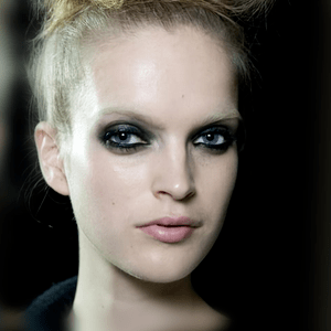
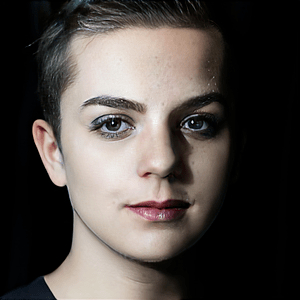
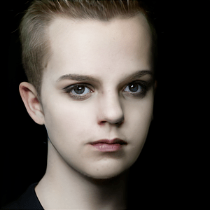
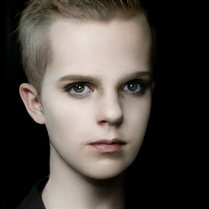
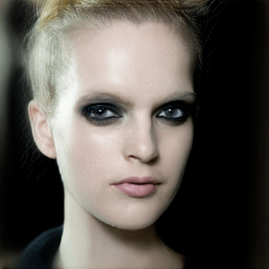
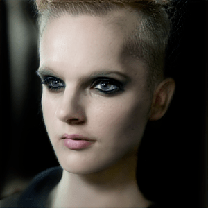
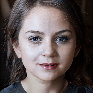
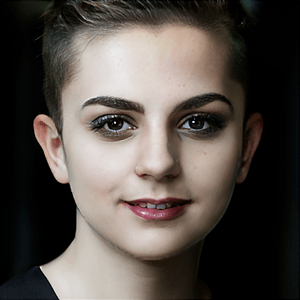
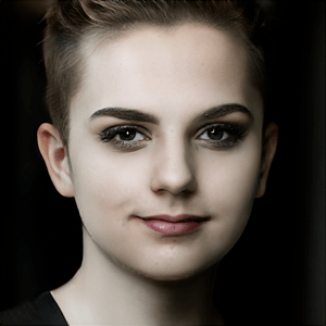
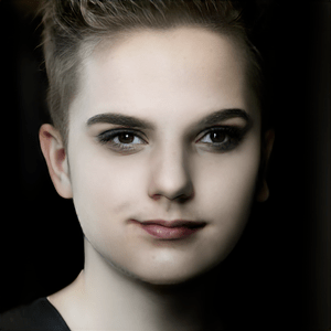
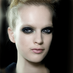
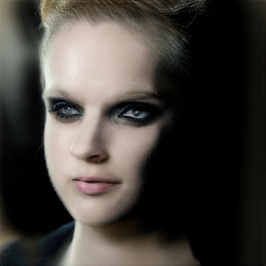
Figure 3: Importance of additional learnable translation parameter. We compare our model(top row) with the model that doesn’t have additional learnable translation parameters(bottom row). The top row shows both gradual changes in head location on the image plane and camera direction, while the other cannot converge to suitable camera rotation.

Appendix C Qualitative Evaluation of Editing

Attr.	$\gamma$	SG2	SG2 $\mathcal{W}+$	PTI	SG2†	SG2† $\mathcal{W}+$	PTI†	Ours
Age	-3.6	-7.320	-6.598	-6.625	-6.522	-6.228	-6.831	-7.146
	-2.4	-5.455	-4.804	-4.526	-4.834	-4.518	-4.726	-4.922
	-1.2	-3.02	-2.557	-2.3	-2.737	-2.476	-2.518	-2.584
	0	0	0	0	0	0	0	0
	1.2	3.142	2.696	2.656	3.141	3.075	2.570	2.725
	2.4	6.464	5.74	5.506	6.686	6.414	5.574	5.929
	3.6	9.868	8.926	8.558	10.267	10.077	8.668	9.296
Smile	-2	-3.150	-2.392	-2.715	-2.627	-2.111	-2.107	-2.711
	-1.33	-2.210	-1.597	-1.838	-1.829	-1.501	-1.447	-1.882
	-0.67	-1.129	-0.798	-0.920	-0.940	-0.764	-0.714	-0.937
	0	0	0	0	0	0	0	0
	0.66	0.964	0.817	0.850	0.831	0.711	0.608	0.919
	1.33	1.925	1.583	1.734	1.558	1.271	1.364	1.854
	2	2.762	2.226	2.524	2.189	1.861	1.962	2.694

(a) Quantitative evaluation of manipulation capability

(b) Quantitative evaluation of identity preservation

Table 1: Quantitative evaluation of editability. In (a), we apply varying magnitudes $\gamma$ of age edit and smile edit to the latent codes acquired by each method and measure the amount of age change and difference of smile extent respectively. In (b), we also compare the identity similarity between the original image and edited images.

A well-performed semantic edit should preserve the original identity of the object while performing meaningful modifications to the desired attributes and that attributes only. From the latent code and camera pose derived by each inversion method, we first evaluate the editing capabilities by manipulating an attribute with the same magnitude and measuring the amount of variation between the original image and the edited image. While camera pose editing is a standard attribute to compare latent space manipulation, viewpoint editing cannot be used to compare the different methods as the generator in question controls geometric attributes explicitly. Instead, we chose age and smile for the attributes to compare latent space manipulation, using the trait-specific estimators, DEX VGG [42] for age and the face attribute classifier used in [30] for smile. The results are shown in Table 1(a). On the other hand, an ideal manipulation of the acquired latent code should achieve not only high editing ability but also high identity preservation for the unchanged attributes. For each inversion method, we compute the identity similarity between the original and edited images for different editing magnitudes. As before, we use the CurricularFace method [22] to calculate identity similarity. The results are shown in Table 1(b).

Appendix D Additional Experimental Results

Following the baseline comparison in our main paper, we provide additional inversion results in Fig. 6 and also provide random viewpoints using the acquired latent code. Fig. 7, Fig. 8 and Fig. 9 applies our inversion method on multiple facial datasets, and we demonstrate the effectiveness of 3D GAN inversion by providing the reconstructed mesh and novel views using the acquired latent code. Fig. 10 depicts our reconstruction ability on non-facial domain, namely cats in the AnimalFace10 dataset.

Finally, additional GANspace [18] editing results can be found in Fig. 12 and Fig. 12, where we use the edited latent code to generate 3D mesh and novel views and prove our method is capable of 3D shape editing.

Input	Ours	SG2	SG2 $\mathcal{W}+$	PTI	SG2†	SG2† $\mathcal{W}+$	PTI†

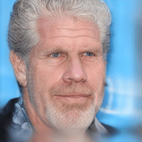
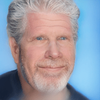
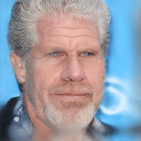
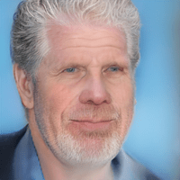
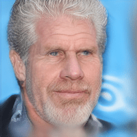
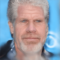
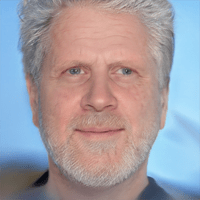
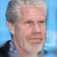
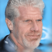
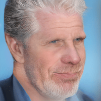
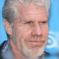
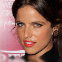
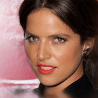
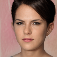
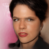
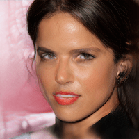
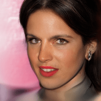
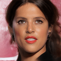
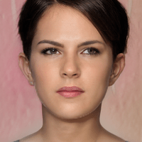
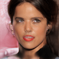
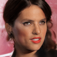
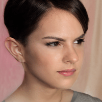
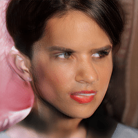
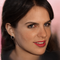
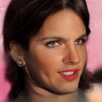
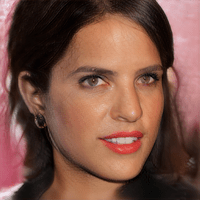
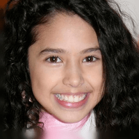
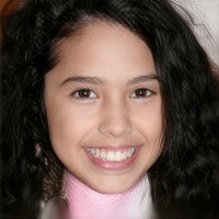
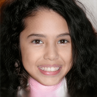
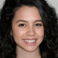
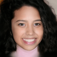
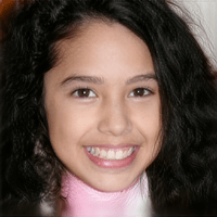
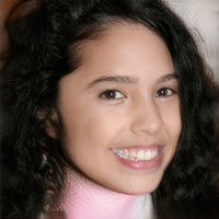
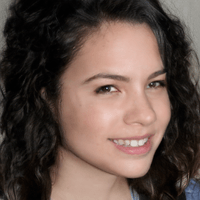
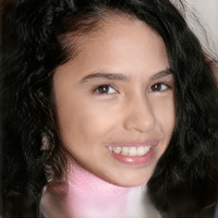
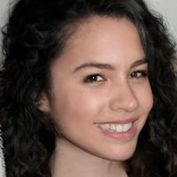
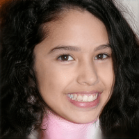
Figure 6: Additional ablation studies on CelebA-HQ [24, 32] dataset

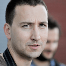
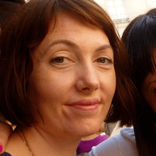
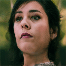
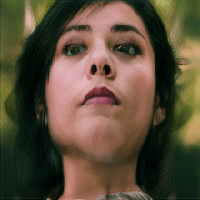
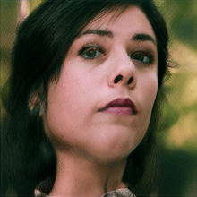
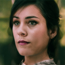
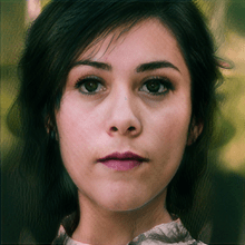
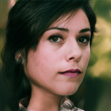
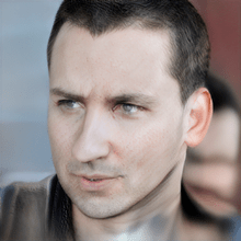
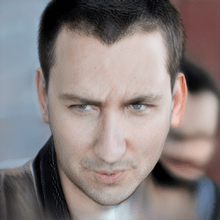
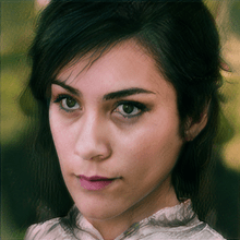
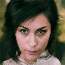
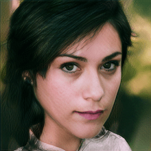
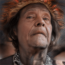
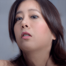
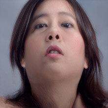
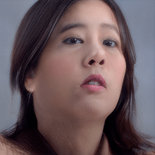
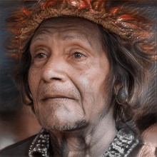
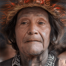
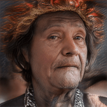
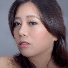
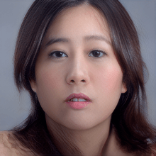
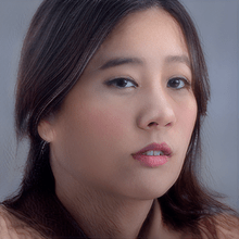
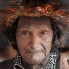
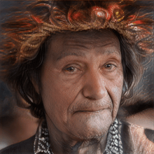
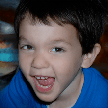
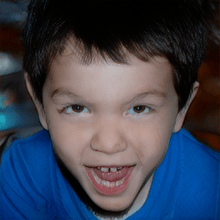
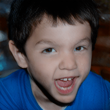
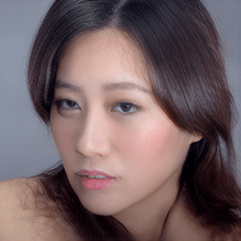
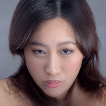
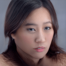
Figure 7: Additional qualitative results on in-domain dataset FFHQ [25]

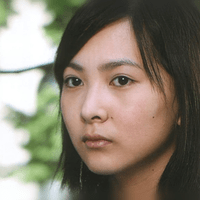
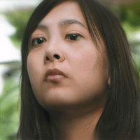
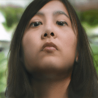
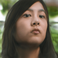
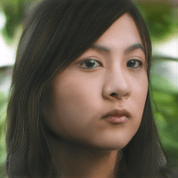
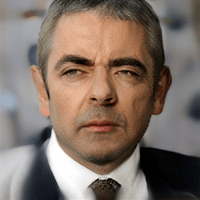
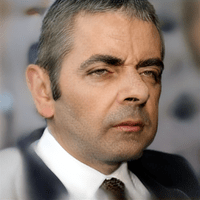
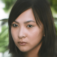
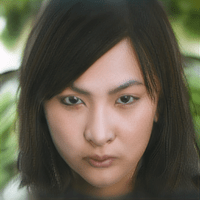
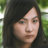
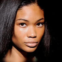
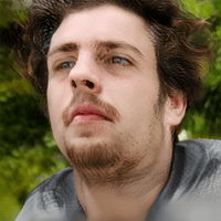
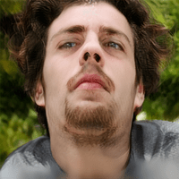
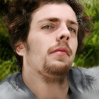
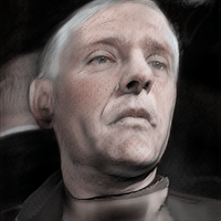
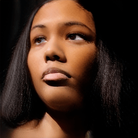
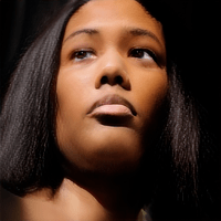
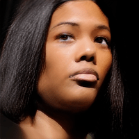
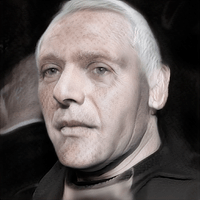
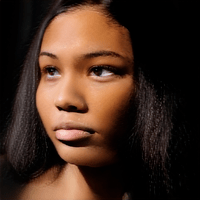
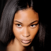
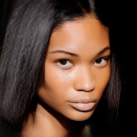
Figure 8: Additional qualitative results on out-of-domain dataset CelebA-HQ [24, 32]

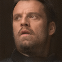
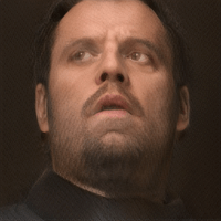
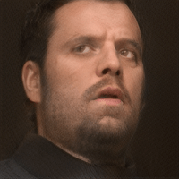
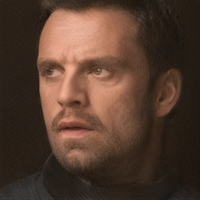
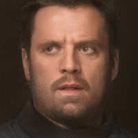
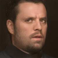
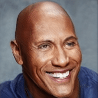
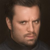
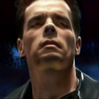
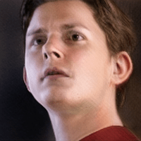
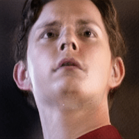
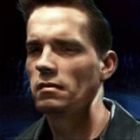
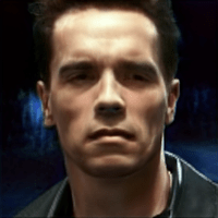
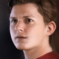
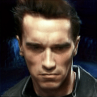
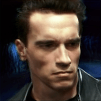
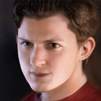
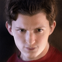
Figure 9: Movie Scene Novel view synthesis with 3D GAN Inversion. We crop facial images from numerous famous movies and invert them into the latent space of EG3D [7]. We demonstrate novel view synthesis of these facial images along with visualization of 3D reconstructed mesh.

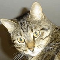
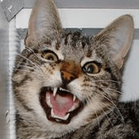
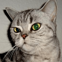
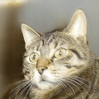
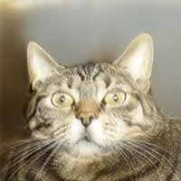
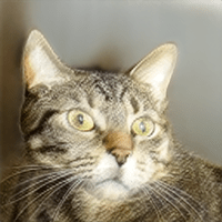
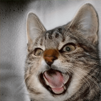
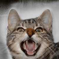
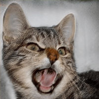
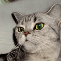
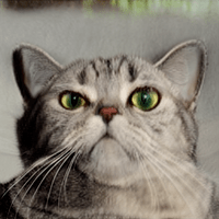
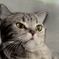
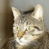
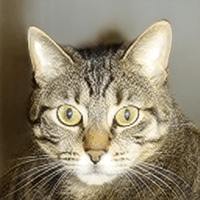
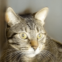
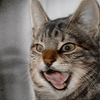
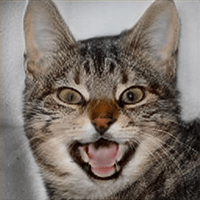
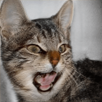
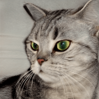
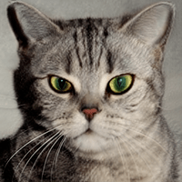
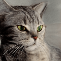
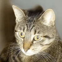
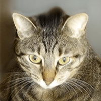
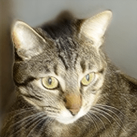
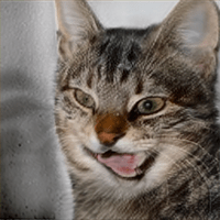
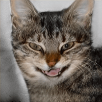
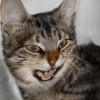
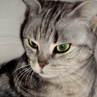
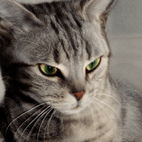
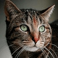
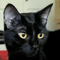
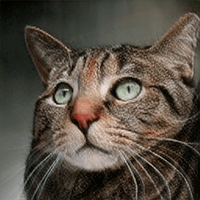
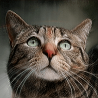
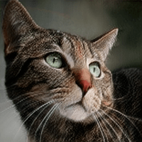
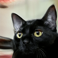
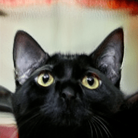
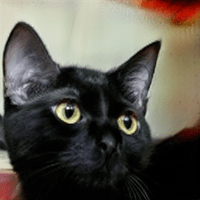
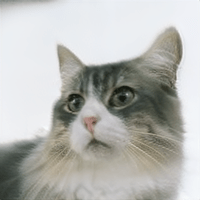
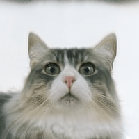
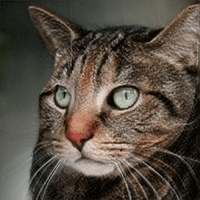
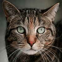
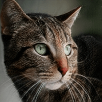
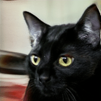
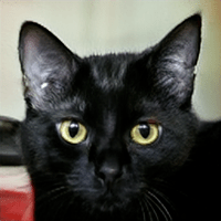
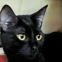
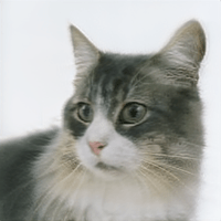
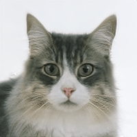
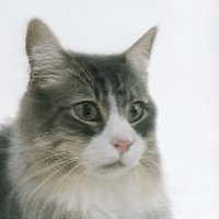
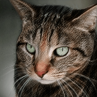
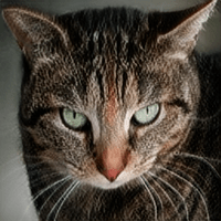
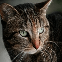
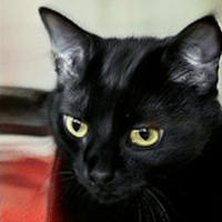
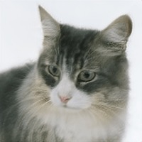
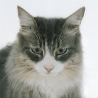
Figure 10: Additional qualitative results on out-of-domain dataset AnimalFace10 dataset [31]

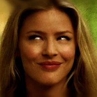
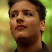
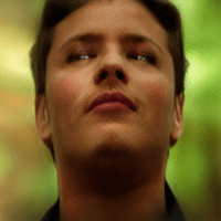
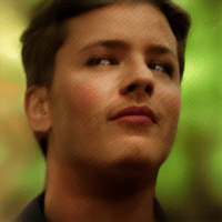
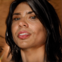
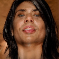
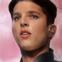
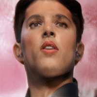
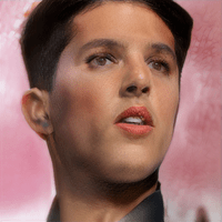
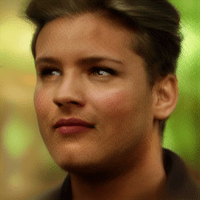
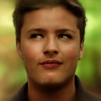
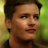
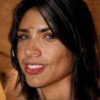
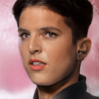
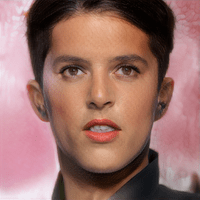
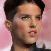
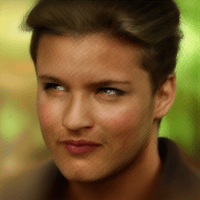
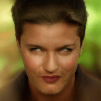
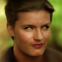
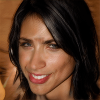
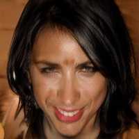
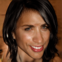
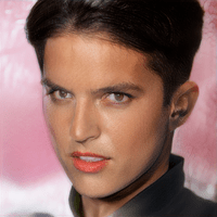
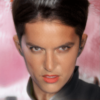
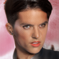
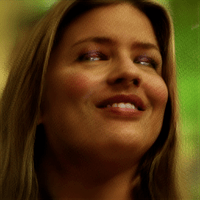
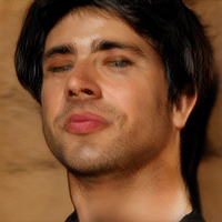
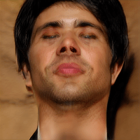
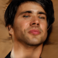
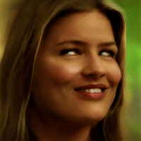
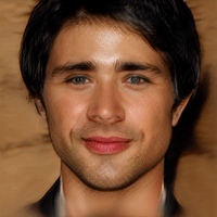
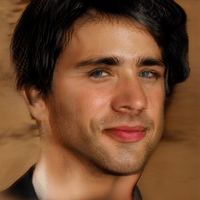
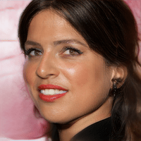
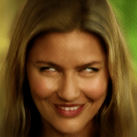
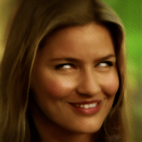
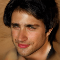
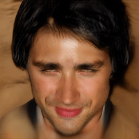
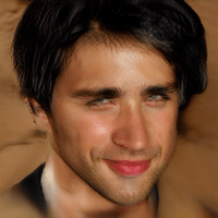
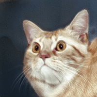
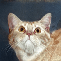
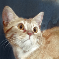
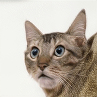
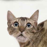
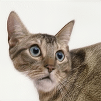
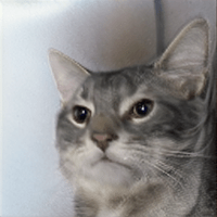
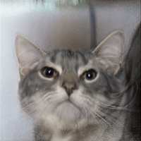
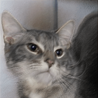
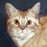
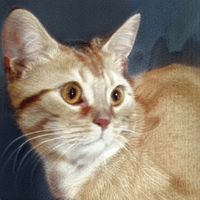
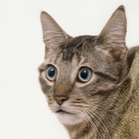
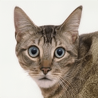
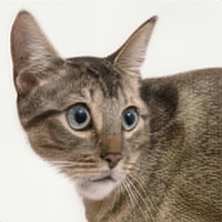
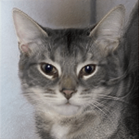
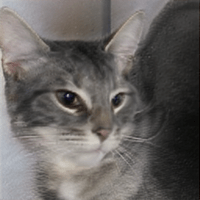
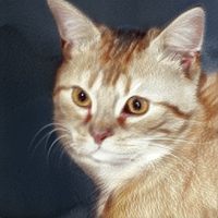
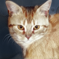
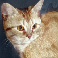
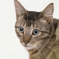
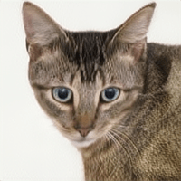
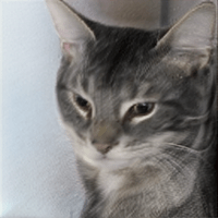
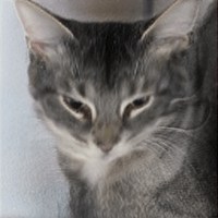
Figure 11: 3D facial Editing. We demonstrate the style-aware geometry editing: gender(first row) and smile(second row).

Figure 12: Editing of cats in AnimalFace10 dataset [31] We evaluate 3D-aware edits: pupil size, and demonstrate our method enables latent-based editing for domains other than human face.

References

- [1] Rameen Abdal, Yipeng Qin, and Peter Wonka. Image2stylegan: How to embed images into the stylegan latent space? In ICCV, 2019.
- [2] Rameen Abdal, Peihao Zhu, Niloy J. Mitra, and Peter Wonka. Styleflow: Attribute-conditioned exploration of stylegan-generated images using conditional continuous normalizing flows. ACM Trans. Graph., 2021.
- [3] Yuval Alaluf, Or Patashnik, and Daniel Cohen-Or. Restyle: A residual-based stylegan encoder via iterative refinement. In Proceedings of the IEEE/CVF International Conference on Computer Vision, pages 6711–6720, 2021.
- [4] Yuval Alaluf, Omer Tov, Ron Mokady, Rinon Gal, and Amit Bermano. Hyperstyle: Stylegan inversion with hypernetworks for real image editing. In CVPR, 2022.
- [5] David Bau, Jun-Yan Zhu, Jonas Wulff, William Peebles, Hendrik Strobelt, Bolei Zhou, and Antonio Torralba. Seeing what a gan cannot generate. In ICCV, 2019.
- [6] Shengqu Cai, Anton Obukhov, Dengxin Dai, and Luc Van Gool. Pix2nerf: Unsupervised conditional p-gan for single image to neural radiance fields translation. In CVPR, 2022.
- [7] Eric R. Chan, Connor Z. Lin, Matthew A. Chan, Koki Nagano, Boxiao Pan, Shalini De Mello, Orazio Gallo, Leonidas Guibas, Jonathan Tremblay, Sameh Khamis, Tero Karras, and Gordon Wetzstein. Efficient geometry-aware 3D generative adversarial networks. In CVPR, 2022.
- [8] Yunjey Choi, Youngjung Uh, Jaejun Yoo, and Jung-Woo Ha. Stargan v2: Diverse image synthesis for multiple domains. In CVPR, 2020.
- [9] Antonia Creswell and Anil Anthony Bharath. Inverting the generator of a generative adversarial network. IEEE Transactions on Neural Networks and Learning Systems, 2019.
- [10] Giannis Daras, Wen-Sheng Chu, Abhishek Kumar, Dmitry Lagun, and Alexandros G Dimakis. Solving inverse problems with nerfgans. arXiv preprint arXiv:2112.09061, 2021.
- [11] Yu Deng, Jiaolong Yang, Jianfeng Xiang, and Xin Tong. Gram: Generative radiance manifolds for 3d-aware image generation. In CVPR, 2022.
- [12] Yu Deng, Jiaolong Yang, Sicheng Xu, Dong Chen, Yunde Jia, and Xin Tong. Accurate 3d face reconstruction with weakly-supervised learning: From single image to image set. In CVPRW, 2019.
- [13] Tan M. Dinh, Anh Tuan Tran, Rang Nguyen, and Binh-Son Hua. Hyperinverter: Improving stylegan inversion via hypernetwork. In CVPR, 2022.
- [14] Yao Feng, Haiwen Feng, Michael J. Black, and Timo Bolkart. Learning an animatable detailed 3D face model from in-the-wild images. SIGGRAPH, 2021.
- [15] Ian Goodfellow, Jean Pouget-Abadie, Mehdi Mirza, Bing Xu, David Warde-Farley, Sherjil Ozair, Aaron Courville, and Yoshua Bengio. Generative adversarial nets. NeurIPS, 2014.
- [16] Jiatao Gu, Lingjie Liu, Peng Wang, and Christian Theobalt. Stylenerf: A style-based 3d aware generator for high-resolution image synthesis. In ICLR, 2022.
- [17] Shanyan Guan, Ying Tai, Bingbing Ni, Feida Zhu, Feiyue Huang, and Xiaokang Yang. Collaborative learning for faster stylegan embedding. arXiv preprint arXiv:2007.01758, 2020.
- [18] Erik Härkönen, Aaron Hertzmann, Jaakko Lehtinen, and Sylvain Paris. Ganspace: Discovering interpretable gan controls. In NeurIPS, 2020.
- [19] Kaiming He, Xiangyu Zhang, Shaoqing Ren, and Jian Sun. Deep residual learning for image recognition. In CVPR, 2016.
- [20] Martin Heusel, Hubert Ramsauer, Thomas Unterthiner, Bernhard Nessler, and Sepp Hochreiter. Gans trained by a two time-scale update rule converge to a local nash equilibrium. In NeurIPS, 2017.
- [21] Heng-Wei Hsu, Tung-Yu Wu, Sheng Wan, Wing Hung Wong, and Chen-Yi Lee. Quatnet: Quaternion-based head pose estimation with multiregression loss. IEEE Transactions on Multimedia, 2019.
- [22] Yuge Huang, Yuhan Wang, Ying Tai, Xiaoming Liu, Pengcheng Shen, Shaoxin Li, Jilin Li, and Feiyue Huang. Curricularface: Adaptive curriculum learning loss for deep face recognition. In CVPR, 2020.
- [23] Max Jaderberg, Karen Simonyan, Andrew Zisserman, and koray kavukcuoglu. Spatial transformer networks. In NeurIPS, 2015.
- [24] Tero Karras, Timo Aila, Samuli Laine, and Jaakko Lehtinen. Progressive growing of gans for improved quality, stability, and variation. arXiv preprint arXiv:1710.10196, 2017.
- [25] Tero Karras, Samuli Laine, and Timo Aila. A style-based generator architecture for generative adversarial networks. In CVPR, 2019.
- [26] Tero Karras, Samuli Laine, Miika Aittala, Janne Hellsten, Jaakko Lehtinen, and Timo Aila. Analyzing and improving the image quality of stylegan. In CVPR, 2020.
- [27] Tero Karras, Samuli Laine, Miika Aittala, Janne Hellsten, Jaakko Lehtinen, and Timo Aila. Analyzing and improving the image quality of StyleGAN. In CVPR, 2020.
- [28] Jeong-gi Kwak, Yuanming Li, Dongsik Yoon, Donghyeon Kim, David Han, and Hanseok Ko. Injecting 3d perception of controllable nerf-gan into stylegan for editable portrait image synthesis. arXiv preprint arXiv:2207.10257, 2022.
- [29] Connor Z Lin, David B Lindell, Eric R Chan, and Gordon Wetzstein. 3d gan inversion for controllable portrait image animation. arXiv preprint arXiv:2203.13441, 2022.
- [30] Ji Lin, Richard Zhang, Frieder Ganz, Song Han, and Jun-Yan Zhu. Anycost gans for interactive image synthesis and editing. In CVPR, 2021.
- [31] Ming-Yu Liu, Xun Huang, Arun Mallya, Tero Karras, Timo Aila, Jaakko Lehtinen, and Jan Kautz. Few-shot unsupervised image-to-image translation. In ICCV, 2019.
- [32] Ziwei Liu, Ping Luo, Xiaogang Wang, and Xiaoou Tang. Deep learning face attributes in the wild. In ICCV, 2015.
- [33] William E Lorensen and Harvey E Cline. Marching cubes: A high resolution 3d surface construction algorithm. SIGGRAPH, 1987.
- [34] Ben Mildenhall, Pratul P. Srinivasan, Matthew Tancik, Jonathan T. Barron, Ravi Ramamoorthi, and Ren Ng. Nerf: Representing scenes as neural radiance fields for view synthesis. In ECCV, 2020.
- [35] Thu Nguyen-Phuoc, Chuan Li, Lucas Theis, Christian Richardt, and Yong-Liang Yang. Hologan: Unsupervised learning of 3d representations from natural images. In ICCV, 2019.
- [36] Michael Niemeyer, Jonathan T. Barron, Ben Mildenhall, Mehdi S. M. Sajjadi, Andreas Geiger, and Noha Radwan. Regnerf: Regularizing neural radiance fields for view synthesis from sparse inputs. In CVPR, 2022.
- [37] Michael Niemeyer and Andreas Geiger. Giraffe: Representing scenes as compositional generative neural feature fields. In CVPR, 2021.
- [38] Or Patashnik, Zongze Wu, Eli Shechtman, Daniel Cohen-Or, and Dani Lischinski. Styleclip: Text-driven manipulation of stylegan imagery. In ICCV, 2021.
- [39] Alec Radford, Jong Wook Kim, Chris Hallacy, Aditya Ramesh, Gabriel Goh, Sandhini Agarwal, Girish Sastry, Amanda Askell, Pamela Mishkin, Jack Clark, et al. Learning transferable visual models from natural language supervision. In PMLR, 2021.
- [40] Elad Richardson, Yuval Alaluf, Or Patashnik, Yotam Nitzan, Yaniv Azar, Stav Shapiro, and Daniel Cohen-Or. Encoding in style: a stylegan encoder for image-to-image translation. In CVPR, 2021.
- [41] Daniel Roich, Ron Mokady, Amit H Bermano, and Daniel Cohen-Or. Pivotal tuning for latent-based editing of real images. ACM Trans. Graph., 2021.
- [42] Rasmus Rothe, Radu Timofte, and Luc Van Gool. Dex: Deep expectation of apparent age from a single image. In ICCVW, 2015.
- [43] Katja Schwarz, Yiyi Liao, Michael Niemeyer, and Andreas Geiger. Graf: Generative radiance fields for 3d-aware image synthesis. In NeurIPS, 2020.
- [44] Katja Schwarz, Axel Sauer, Michael Niemeyer, Yiyi Liao, and Andreas Geiger. Voxgraf: Fast 3d-aware image synthesis with sparse voxel grids. arXiv preprint arXiv:2206.07695, 2022.
- [45] Yujun Shen, Jinjin Gu, Xiaoou Tang, and Bolei Zhou. Interpreting the latent space of gans for semantic face editing. In CVPR, 2020.
- [46] Ivan Skorokhodov, Sergey Tulyakov, Yiqun Wang, and Peter Wonka. Epigraf: Rethinking training of 3d gans. arXiv preprint arXiv:2206.10535, 2022.
- [47] Omer Tov, Yuval Alaluf, Yotam Nitzan, Or Patashnik, and Daniel Cohen-Or. Designing an encoder for stylegan image manipulation. ACM, 2021.
- [48] Roberto Valle, José M Buenaposada, and Luis Baumela. Multi-task head pose estimation in-the-wild. TPAMI, 2020.
- [49] Zhou Wang, Eero P Simoncelli, and Alan C Bovik. Multiscale structural similarity for image quality assessment. In ACSSC. Ieee, 2003.
- [50] Jianfeng Xiang, Jiaolong Yang, Yu Deng, and Xin Tong. Gram-hd: 3d-consistent image generation at high resolution with generative radiance manifolds. arXiv preprint arXiv:2206.07255, 2022.
- [51] Yinghao Xu, Sida Peng, Ceyuan Yang, Yujun Shen, and Bolei Zhou. 3d-aware image synthesis via learning structural and textural representations. In CVPR, 2022.
- [52] Oğuz Kaan Yüksel, Enis Simsar, Ezgi Gülperi Er, and Pinar Yanardag. Latentclr: A contrastive learning approach for unsupervised discovery of interpretable directions. In ICCV, 2021.
- [53] Richard Zhang, Phillip Isola, Alexei A. Efros, Eli Shechtman, and Oliver Wang. The unreasonable effectiveness of deep features as a perceptual metric. In CVPR, 2018.
- [54] Peng Zhou, Lingxi Xie, Bingbing Ni, and Qi Tian. Cips-3d: A 3d-aware generator of gans based on conditionally-independent pixel synthesis. arXiv preprint arXiv:2110.09788, 2021.
- [55] Tinghui Zhou, Matthew Brown, Noah Snavely, and David G. Lowe. Unsupervised learning of depth and ego-motion from video. In CVPR, 2017.
- [56] Yi Zhou, Connelly Barnes, Jingwan Lu, Jimei Yang, and Hao Li. On the continuity of rotation representations in neural networks. In CVPR, June 2019.
- [57] Jiapeng Zhu, Yujun Shen, Deli Zhao, and Bolei Zhou. In-domain gan inversion for real image editing. In ECCV, 2020.
- [58] Jun-Yan Zhu, Philipp Krähenbühl, Eli Shechtman, and Alexei A. Efros. Generative visual manipulation on the natural image manifold. In ECCV, 2016.
- [59] Peihao Zhu, Rameen Abdal, Yipeng Qin, John Femiani, and Peter Wonka. Improved stylegan embedding: Where are the good latents?, 2020.