Deep learning waveform anomaly detector for numerical relativity catalogs

Abstract

Numerical Relativity has been of fundamental importance for studying compact binary coalescence dynamics, waveform modelling, and eventually for gravitational waves observations. As the sensitivity of the detector network improves, more precise template modelling will be necessary to guarantee a more accurate estimation of astrophysical parameters. To help improving the accuracy of numerical relativity catalogs, we developed a deep learning model capable of detecting anomalous waveforms. We analyzed 1341 binary black hole simulations from the SXS catalog with various mass-ratios and spins, considering waveform dominant and higher modes. In the set of waveform analyzed, we found and categorised seven types of anomalies appearing close to the merger phase.

I Introduction

The network of gravitational wave (GW) detectors composed by the two LIGO Aasi et al. (2015) and Virgo Acernese et al. (2015) observatories has already completed three successful observation runs Abbott et al. (2021), with the detection of over 90 coalescences of compact binary systems. To maximize the possibility of detections and their (astro-)physics output, collected data are analyzed via matched-filtering techniques Wainstein and Zubakov (1962); Abbott et al. (2020a) by correlating them with pre-computed waveform templates, whose development is the object of intense investigation Pratten et al. (2021, 2020); García-Quirós et al. (2021, 2020); Ossokine et al. (2020); Babak et al. (2017); Pan et al. (2014). Improving the accuracy of GW templates straightforwardly enhances the quality of astrophysical information obtained from these sources.

Waveforms can be expressed as time series resulting from the spin-weighted spherical harmonic decomposition of the gravitational wave strain. While the dominant, quadrupolar mode of GW templates has been enough to analyze the vast majority of signals, in a few cases the imprints of sub-dominant (or higher modes, HM henceforth) have been detected Abbott et al. (2020b, c). With increasing sensitivity and widening the network of observatories in future observation runs with KAGRA Abe et al. (2022), it is expected that HM will have a larger impact on the detected signals Pürrer and Haster (2020). GW waveforms generated via Numerical Relativity (NR) simulations Scheel et al. (2009) have been widely used for construction of semi-analytical and phenomenological templates, and have produced accurate HM waveforms over a vast parameter space.

The goal of the present paper is to provide a new tool to assess the data quality of the various simulations presented in a NR catalog. The numerical codes’ complexity and the simulations’ long runtime can generate a systematic accumulation of numerical residuals, leading to defects in the morphology of the waveforms. Furthermore, there are cases in which a catalog presents simulations with different numerical resolutions due to code updating.

In this work, we developed the deep learning model Waveform AnomaLy DetectOr (WALDO), capable of signaling possible anomalous waveforms in a NR catalog Pereira (2022). In our searches within binary black hole (BBH) simulations, we categorized seven different types of anomalies during the stages of coalescence. Identifying and excluding such waveforms is critical to the quality of research in GW analysis and surrogate modeling Varma et al. (2019a).

Applications of deep learning models to gravitational wave data is not new Easter et al. (2019); Gabbard et al. (2018); Varma et al. (2019b); Shen et al. (2019); Rebei et al. (2019); Setyawati et al. (2020); Haegel and Husa (2020); Cuoco et al. (2021); Green et al. (2020); Ormiston et al. (2020); Yu and Adhikari (2021); Schmidt et al. (2021); Gabbard et al. (2021); Fragkouli et al. (2022); Yan et al. (2022), but to the best of our knowledge this is the first work using deep learning to check the consistency of numerical simulations.

The paper is structured as follows. Section II is intended to help the reader providing a reference to our notations, Section III describes the dataset we used for our analysis, and Section IV describes our machine learning-based process to identify anomalous waveforms, whose results are presented in Section V. Finally we summarize our conclusions in Section VI.

II Definitions

We adopt geometric units $G=c=1$, and we denote by $u$ the dimension-less time obtained by dividing physical time by the total mass $M$ of the binary system, whose zero is set by the epoch of the peak of the dominant mode amplitude. The BBH mass-ratio $q$ is taken to be larger than 1, the dimensionless spins $\vec{\chi}_{i}\equiv\vec{S}_{i}/M^{2}$, $i=\{1,2\}$, being $\vec{S}_{i}$ the standard spin and the orbital eccentricity is denoted by $e$. From the GW strain, i.e. the GW polarization complex combination $h_{+}-ih_{\times}$, we extract (and rescale as usual by distance $r$ and mass $M$) spherical harmonic modes $h_{lm}(t)$, indexed by integers $l\geq 2$, $|m|\leq l$, resulting from the decomposition on the spin-weighted spherical harmonics base ${}_{-2}Y_{lm}$ of the strain,

$$h_{lm}(t)=\int d\Omega\,\left(h_{+}-ih_{\times}\right)(\theta,\phi)\,_{-2}Y_{lm}(\theta,\,\phi)\,,$$ (1)

where $\Omega$ is the solid angle parametrized by $\theta$ and $\phi$, which are respectively the angle between the radiation direction and the normal to the orbital plane, and a phase corresponding to a rotation in the orbital plane.

III The dataset

We create a dataset using 1341 BBH simulations from the Simulating eXtreme Spacetimes (SXS) catalog Scheel et al. (2009), whose parameters are in the region $q=[1.0:4.0]$, $|\vec{\chi}_{i}|=[-0.9:0.9]$, and $e\simeq[0.0:8.0\times 10^{-4}]$ et al. (2013, 2019). All simulation names are listed in the WALDO’s repository Pereira (2022). Considering the modes $(l\leq 4,\,l-1\leq|m|\leq l)$, in total our dataset is composed by $N_{d}=8046$ waveforms. Figure 1 shows the parameter space distribution of eccentricity, spin-aligned parameter $\chi_{eff}$, spin-precession parameter $\chi_{p}$ Apostolatos et al. (1994); Green et al. (2021) and the mass-ratio $q$.

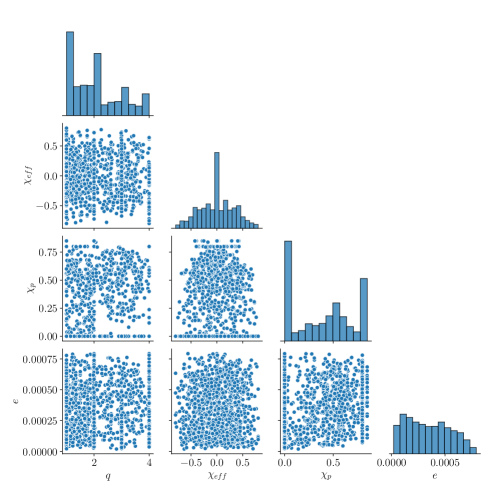
Figure 1: Representation of the parameter space of the 1341 simulations: corner plot of the distribution of eccentricity $e$, mass-ratio $q$, spin-aligned parameter $\chi_{eff}$ and spin-precession $\chi_{p}$.

To facilitate a unified treatment of all waveforms, we cut the waveforms to the highest initial time value of the entire dataset, i.e., the inspiral starts at $u=-1700$, with corresponding instantaneous frequency for the dominant mode $f_{min}\simeq 14-19Hz\left(M/100M_{\odot}\right)^{-1}$, depending on the mass ratio. This conditioning is necessary to guarantee the same resolution of the waveforms – with the same time intervals – during the neural network (NN) training.

Also, we find it convenient to re-sample all modes via the time-reparametrization

$$\begin{array}[]{rcl}u^{\prime}(u)&=&\displaystyle c_{1}\,r(u)+c_{2}\,,\\ r(u)&=&\displaystyle\tanh\left[a\left(u-u_{0}+b\right)\right]\,,\\ c_{1}&=&\displaystyle\left(u_{F}-u_{0}\right)/\left[r(u_{F})-r(u_{0})\right]\,,\\ c_{2}&=&\displaystyle u_{0}-c_{1}\,r(u_{0})\,,\end{array}$$ (6)

where $u_{0}$ and $u_{F}$ are the initial and final value of the dimension-less time $u=[-1700:100]$; $a=5\times 10^{-4}$ and $b=5.\times 10^{2}$ are constants. The rationale for this parameterization is to make smoother the transition from the wider spacing during the inspiral to a smaller one in the merger-ringdown phase, while keeping the number of samples equal to $N_{s}=2048$ for all waveforms, without degrading the sampling rate in the merger-ringdown phase.

For deep learning feature engineering – the pre-processing procedures for improving NN computations – we normalize the dataset with the highest waveform amplitude value,

$$h_{lm}^{(k)} \rightarrow h_{lm}^{(k)}/\max\left(|h_{22}^{(k)}|\right)\,,$$ (7)

where the index $(k)$ denotes the simulation number, $k=[1:8046]$. We define the dataset as the numerical three-dimensional array,

$${\bf X} \equiv \left(\mathit{Re}\left\{h_{lm}\right\},\mathit{Im}\left\{h_{lm}\right\}\right)^{(k)}\,,$$ (8)

whose dimensionality is $(N_{d},\,N_{s},2)$.

IV WALDO

The Waveform AnomaLy DetectOr (WALDO) holds a U-Net architecture Ronneberger et al. (2015), where the waveform input $X^{(k)}$ is reproduced as the output $\bar{X}^{(k)}$. During the training, the model learns all possible waveform features related to the parameter space. Evaluating its performance with the mismatch $\mathcal{M}$ between $h_{lm}^{(k)}$ and its prediction $\bar{h}_{lm}^{(k)}$, the measurement of high mismatch values can flag the presence of waveforms whose morphology do not match the dataset one, i.e., we can find anomalous waveforms. The mismatch is defined as $\mathcal{M}\equiv 1-\mathcal{O}$, where ${\cal O}$ denotes the match between two time series $h_{1,2}$, defined in terms of the scalar product

$$\langle h_{1}|h_{2}\rangle=2\int_{0}^{\infty}\left(\tilde{h}_{1}(f)\tilde{h}_{2}^{*}(f)+\tilde{h}_{2}(f)\tilde{h}_{1}^{*}(f)\right)df\,,$$ (9)

where $f$ is variable conjugate to time under Fourier transform $h\to\tilde{h}$, the match being defined by maximization over initial phase and time of the scalar product of normalized waveforms

$$\mathcal{O}\equiv\stackrel{{\scriptstyle Max}}{{t,\phi_{0}}}\frac{\langle h_{1}|h_{2}\rangle}{\left(\langle h_{1}|h_{1}\rangle\langle h_{2}|h_{2}\rangle\right)^{1/2}}\,.$$ (10)

The WALDO’s encoder part presents convolutional layers of $\emph{kernel-size}=3$ intermediated by max-pooling layers with $\emph{pool-size}=2$. The input dimensionality reduces as the number of channels $C$ increases for $C=[32,\,64,\,128,\,256,\,512]$. The decoder part duplicates the layers’ dimension with up-sampling layers, followed by convolutional, concatenation, and another convolutional layer. We compose the architecture with ReLU activation functions, except for the hyperbolic tangent in the output layer.

IV.1 Training and validation

To examine the training performance, we split the dataset into 70% for training data, which is computed in parallel with 20% for validation data, and 10% for testing data. Since 8046 waveforms forms a small dataset, we use the K-fold validation method for $K=3$, and $\emph{batch-size}=1$. We minimize the model parameters using the mean squared error loss function and Adagrad optimizer Duchi et al. (2011). During the validation, the NN can be trained through 200 epochs without over-fitting. We retrain the model using 90% of the dataset and obtain the mean square error average $2.8\times 10^{-7}$ over the testing data.

V Results

After the training, WALDO evaluates the mismatch and packs the values with $(l,\,m)$ mode labels, together with the identification simulation number (ID) – that comes from the SXS simulation names as SXS:BBH:ID – the parameter space $\left(q,\,\vec{\chi}_{1},\,\vec{\chi}_{2},\,e\right)^{(k)}$, the waveforms $h_{lm}^{(k)}$ and their predictions $\bar{h}_{lm}^{(k)}$. Creating a histogram for each mode $(l,\,m)$, we isolated 1% of the highest mismatch waveforms to verify any possible morphological discrepancy in the predictions. Figure 2 shows the $(3,\,2)$ waveform mismatch distribution of average $1.26\times 10^{-5}$ represented by the vertical green line; the $quantile=0.99$, marked by the vertical pink line, separates 14 simulations that call for examination. The lowest mismatch value is on the order of $5.0\times 10^{-6}$ due to the low number of simulations $N_{d}=1341$ and varied waveform morphology. We reinforce that the NN training is usually done with hundreds of thousands of data, however our small dataset does not interfere with the quality of waveform reproduction.

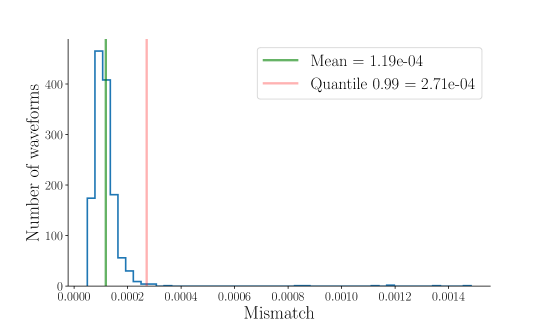
Figure 2: Mismatch histogram of 1341 waveforms $h_{32}^{(k)}$ and the predictions $\bar{h}_{32}^{(k)}$. The vertical green line shows the average value $1.26\times 10^{-5}$, and the pink one marks the $quantile=0.99$ with 14 simulations on its right side.

In this case, we found high mismatches due to noise accumulation in the predicted waveforms, even if qualitatively they follow the NR morphological patterns, as shown in Fig. 3 – where the blue line is $h_{32}$, the dashed orange line is $\bar{h}_{32}$, and the green one is $Re\left\{h_{32}-\bar{h}_{32}\right\}$ amplified 10 times. On the other hand, we also found morphological discrepancies between NN predicted and NR waveform modes, confined in specific sectors of the coalescence, causing high mismatches. An irregularity fairly common for the higher modes, is that the mode amplitude around the merger peak has a greater magnitude than expected – what we call the merger-peak (MP) anomaly, as seen in Fig. 4.

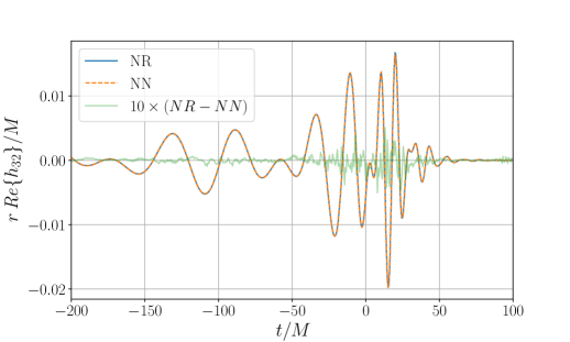
Figure 3: NR vs NN comparison of the $(3,\,2)$-waveforms from the silmulation ID = 1018. $Mismatch=3.0\times 10^{-4}$; $q=1.2$, $\vec{\chi}_{1}=(-0.59,0.15,-0.39)$, $\vec{\chi}_{2}=(-0.73,0.19,0.22)$, and $e=4.2\times 10^{-4}$.

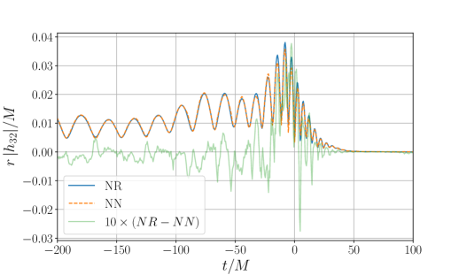
Figure 4: NR vs NN comparison of the $(3,\,2)$-waveforms from the silmulation ID = 1995, displayng a MP anomaly. $Mismatch=1.48\times 10^{-3}$; $q=4.0$, $\vec{\chi}_{1}=(0.51,-0.29,-0.54)$, $\vec{\chi}_{2}=(0.07,0.07,-0.79)$, and $e=1.2\times 10^{-4}$.

For even $m$ modes, we found MP anomalies in $\mathrm{ID}_{(3,2)}=[1863,\,1991-1993,\,1995]$ and $\mathrm{ID}_{(4,4)}=[1982,\,1983,\,1991,\,1992,\,1995]$. In the search for odd $m$ modes, we restrict the mass ratio to $q>1.0$, where we found $\mathrm{ID}_{(2,1)}=[1982,\,1993]$, $\mathrm{ID}_{(3,3)}=[1982,\,1983,\,1989,1991-1993,\,1995]$, and $\mathrm{ID}_{(4,3)}=[0601,\,1982,\,1983,\,1989,\,1991-1993,\,1995]$.

In some waveform $(4,\,4)$ modes the ringdown decay begins a little later in NR simulations than in our NN predictions. Figure 5 shows an example of the lazy-ringdown (LR) anomaly, also found in $\mathrm{ID}_{(4,\,4)}=[0230,\,1477,\,1481,\,2104]$. In the simulation $\mathrm{ID}_{(4,4)}=0155$, on the other hand, the ringdown amplitude does not exhibit appropriate asymptotic behavior. The asymptotic-ringdown (AR) anomaly is shown in Fig. 6.

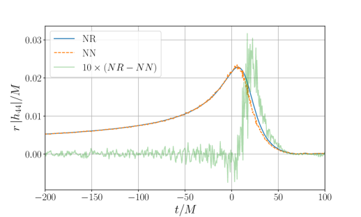
Figure 5: NR vs. NN comparison of the $(4,\,4)$-waveforms from the simulation ID = 0328 displaying a LR anomaly. $Mismatch=1.44\times 10^{-3}$; $q=1.0$, $\vec{\chi}_{1}=(0.0,0.0,0.8)$, $\vec{\chi}_{2}=(0.0,0.0,0.8)$, and $e=1.1\times 10^{-4}$.

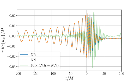
Figure 6: NR vs. NN comparison of the $(4,\,4)$-waveforms from the silmulation ID = 0155 exemplifying a AR anomaly. $Mismatch=1.21\times 10^{-3}$; $q=1.0$, $\vec{\chi}_{1}=(0.0,0.0,0.8)$, $\vec{\chi}_{2}=(0.0,0.0,0.8)$, and $e=5.1\times 10^{-4}$.

V.1 Constraint dataset search

The homogeneity of the parameter space distribution is important to avoid WALDO’s prediction bias. For instance, a dataset containing 500 simulations of spin-aligned BBH and 20 precessing binaries can lead to high mismatch values for waveforms whose features indicate precession.

Thereby, we focus our search for anomalies on $|\vec{\chi}_{1,2}|\leq 0.4$, where we have a higher simulation density. We choose $quantile=0.90$ to isolate 15 waveforms. This constraint leads us to find more AR anomalies in $\mathrm{ID}_{(3,\,3)}=[0116,\,0115,\,0119,\,0129]$ and $\mathrm{ID}_{(4,\,4)}=[0070,\,0115,\,0124,\,0135,\,0150]$. In addition, we found waveforms with similar decay as in Fig. 6, but with non-oscilatory patterns. In this case, those ringdowns were affected by the time interpolation of Eq. 6 because their final time is smaller than $u=70$, giving rise to what we dubbed short-ringdown (SR) anomaly, found in $\mathrm{ID}_{(l,m)}=[1112,\,1114,\,1133]$, for all $(l,m)$. Fig. 7 shows the $h_{22}$ modes from these simulations.

Figure 7: Short-ringdown anomaly in the simulations ID = [1112, 1114, 1133].

The ringdown amplitude of the dominant mode is expected to show a smooth, quasi-exponential decay, however, in the simulations $\mathrm{ID}_{(2,2)}=[0066,\,0067,\,0070,\,0072,\,0126,\,0136]$ appear small ripples up to $u=40$ as in Fig. 8, which we call the rippled-ringdown (RR) anomaly.

Note that these small ripples are present in several of the original NR simulations, and they are reproduced by the NN predictions, however with high enough mismatch to be uncovered.

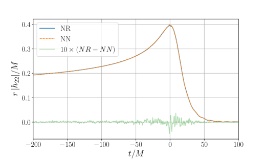
Figure 8: NR vs. NN comparison of the $(2,\,2)$-waveforms from the simulation ID = 0072, showing a RR anomaly. $Mismatch=1.33\times 10^{-5}$ ; $q=1.0$, $\vec{\chi}_{1}=(0.0,0.0,0.0)$, $\vec{\chi}_{2}=(0.0,0.0,0.0)$, and $e=1.5\times 10^{-4}$.

V.2 Radiation field search

In NR the strain modes are computed from the integration of the radiation field $\Psi_{4}$. This operation is not trivial, and it can lead to accumulated numerical noise Reisswig and Pollney (2011). For this reason, we investigate the $\psi_{lm}=\ddot{h}_{lm}$ modes within the whole dataset to ensure whether those anomalies can be ascribed to integration residues.

We retrained the NN and evaluate the mismatch between NR $\psi_{lm}$ waveforms and their reproductions $\bar{\psi}_{lm}$. From previous analyses, we found exclusively MP anomalies in $h_{lm}$ modes with $\mathrm{ID}_{(2,2)}=[1993,\,1995]$, $\mathrm{ID}_{(3,2)}=[1863,\,1878,\,1983,\,1991-1993,\,1995]$, $\mathrm{ID}_{(3,3)}=[1982,\,1989,\,1991-1993]$, $\mathrm{ID}_{(4,3)}=[1103,\,1982,\,1983,\,1989,\,1991-1993]$, and $\mathrm{ID}_{(4,4)}=[0024,0126,1982,1989,1993,1995]$.

Still, the $\psi_{lm}$ modes revealed smaller magnitudes than the predictions in the initial region of the merger as seen in Fig. 9. The initial-merger (IM) anomalies are present in $\psi_{lm}$ with $\mathrm{ID}_{(2,2)}=[1982,\,1989]$, $\mathrm{ID}_{(3,2)}=[1982,\,1989]$, $\mathrm{ID}_{[(3,3),\,(4,3),\,(4,4)]}=1995$.

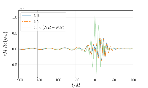
Figure 9: NR vs NN comparison of the $\psi_{32}$ from the silmulation ID = 1989. $Mismatch=2.7\times 10^{-3}$; $q=4.0$, $\vec{\chi}_{1}=(-0.50,-0.29,-0.55)$, $\vec{\chi}_{2}=(0.02,-0.10,-0.79)$, and $e=6.1\times 10^{-4}$.

In the $\psi_{lm}$ mode $(2,\,1)$, we did not find MP or IM anomalies but a qualitatively different discrepancy in $\mathrm{ID}_{(2,1)}=[0013,\,0252,\,0292,\,0388,\,0513,\,0575,\,0464,\,1508,\,2126]$. The dephased-inspiral (DI) anomaly appears as if the NN inspiral was generated by a higher eccentric orbit than the NR one, see e.g. Fig. 10. In fact, simulations with eccentricity $e>1.0\times 10^{-4}$ have to be considered non-negligibly eccentric with respect to the majority of simulations.

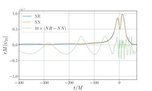
Figure 10: NR vs NN comparison of the $\psi_{21}$ from the simulation ID = 1508, showing a DI anomaly. $Mismatch=2.45\times 10^{-2}$; $q=1.3$, $\vec{\chi}_{1}=(0.0,0.0,0.29)$, $\vec{\chi}_{2}=(0.0,0.0,-0.07)$, and $e=1.6\times 10^{-4}$.

VI Discussion

Anomaly	Description
(AR) Asymptotic-Ringdown	Non-null asymptotic behavior during ringdown.
(LR) Lazy-Ringdown	Ringdown late decay.
(RR) Rippled-Ringdown	Ripples in the dominant mode ringdown amplitude.
(SR) Short-Ringdown	Ringdown with length below $70M$.
(MP) Merger-Peak	Higher amplitude around the merger peak.
(IM) Initial-Merger	Shorter amplitude in the merger beginning.
(DI) Dephased-Inspiral	Oscillatory dephasing during inspiral.

Table 1: Seven waveform anomalies detected by WALDO.

To assess the quality of Numerical Relativity data, and to identify candidate problematic waveforms, we developed Waveform AnomaLy DetectOr (WALDO) wich allowed us to identify potentially anomalous waveforms both in the dominant and higher modes. We trained our model with 8046 waveforms with a U-Net neural architecture and calculated the mismatch between the NR waveforms and the NN predictions. By isolating the 1% waveforms with highest mismatch, we identified seven qualitatively different anomalies during the inspiral, merger, and ringdown stages. Table 1 summarizes the anomaly categories.

The present work intends to be a starting point for a more thorough investigation over neural network applied to numerical waveforms.

Except for the DI anomaly, all others ones are in the waveform merger-ringdown stages, which suggests the need to improve the adaptive mesh refinement method of numerical simulations Berger and Oliger (1984). The more refined the calculations during the collision of black holes, the more accurate the waveform during the merger.

In our search for anomalies in the $\Psi_{4}$ radiative field modes, we did not find LR and AR anomalies, leading us to conclude that these are strain integration issues. We cannot draw the same conclusion about the RR anomaly in $h_{22}$, because of its small magnitude and its disappearing in $\Psi_{4}$, i.e. after double derivatives.

We focus our anomaly search on the $quantile>0.99$ region of the mismatch, and for higher modes with $l\leq 4$.

We highlight that for our analysis the dataset need to be as homogeneous as possible in terms of astrophysical parameter space, to avoid large mismatch values when dealing with anomaly-free waveforms because of poor modeling. It is essential to remove simulations that have anomalies from the dataset and re-train the neural network to ensure that low-quality simulations do not polllute the training set. Such anomalies can impair waveform modeling Khan et al. (2019); Taracchini et al. (2014); Blackman et al. (2015, 2017) and interfere with analysis, such as the ringdown quasi-normal modes Leaver (1985); Maggiore (2008); Yang et al. (2012).

We propose that WALDO can be applied to any timeseries, such as gravitational waves from binary neutron star and back hole-neutron star binary. Also, we suggest to evaluate the quality of new simulations for the next generations of NR codes by comparing them with waveforms from well-established catalogs in the literature.