Asymptotic Properties of Stieltjes Constants

Abstract

We present a new asymptotic formula for the Stieltjes constants which is both simpler and more accurate than several others published in the literature (see e.g. [3], [6], [13]). More importantly, it is also a good starting point for a detailed analysis of some surprising regularities in these important constants.

Keywords: Stieltjes constants, saddle point method, Nørlund–Rice integral

1 Introduction

The Stieltjes constants $\gamma_{n}$ are essentially coefficients of the Laurent series expansion of the Riemann zeta function around its only simple pole at $s=1$:

$$\zeta(s)=\frac{1}{s-1}+{\displaystyle\sum\limits_{n=0}^{\infty}}\frac{\left(-1\right)^{n}}{n!}\gamma_{n}\left(s-1\right)^{n}$$ (1)

It is commonly believed that they are irrational numbers, and even transcendental, however no rigorous proof of this has been given [11]. High precision numerical computations of them are quite a challenge (see [10] and references therein). A common and frequently cited view is that ”for large $n$, the Stieltjes constants grow rapidly in absolute value, and change signs in a complex pattern” [14]. The first view is beyond any doubt, as illustrated in the Figure 1 below.

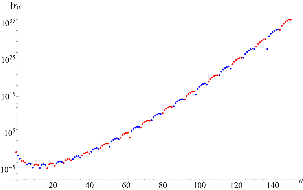
Figure 1: Absolute values of 150 initial Stieltjes coefficients $\gamma_{n}$. Global, fast growing trend is evident. Oscillations of increasing amplitude and decreasing frequency superimposed on this trend are visible. Red dots mean positive values, blue dots mean negative values. The scale on the vertical axis is logarithmic.

In this paper, however, we will show that the second view is incorrect: not only the signs of the Stieltjes constants, but their values also show amazing regularities.

There are three asymptotic formulas for these constants in the literature ([6], [3], [13]). We believe that the one presented in this paper is definitely simpler than the others. It is also more accurate. In particular, it recreates correctly the sign of $\gamma_{n}$ for the particular value of $n=137$ which is usually troublesome for asymptotic formulas. Most importantly, this formula can be a starting point for the analysis of the above-mentioned surprising regularities of Stieltjes constants:

$$\gamma_{n}\sim\sqrt{\frac{2}{\pi}}n!\operatorname{Re}\frac{\Gamma\left(s_{n}\right)e^{-cs_{n}}}{\left(s_{n}\right)^{n}\sqrt{n+s_{n}+\frac{3}{2}}}$$ (2)

where $s_{n}$ is the saddle point (see below):

$$s_{n}=\frac{n+\frac{3}{2}}{W\left(\frac{n+\frac{3}{2}}{2\pi i}\right)}$$ (3)

In formula (2) $c\equiv\ln\left(2\pi i\right)$ is a complex constant and $W$ is the Lambert function (sometimes called the omega function or product logarithm, see [16]).

The basic tool is, as usual in such computations, the saddle point method whereas the starting point is a certain alternating sum, which, due to the still little known Nørlund-Rice formula, can be converted into an integral over the complex contour. As will be shown subsequently, global properties of this integral clearly suggest using the saddle point method.

2 Algorithm for calculating Stieltjes constants

This work is a natural continuation of the previous one [10]. In that work, certain numerically efficient formula for Stieltjes constants was given. In the present work, we will use this formula to derive a new, effective formula for asymptotics for these important constants. As it was done in [10], we will use polynomial interpolation for the (regularized) Riemann zeta function $\varphi(s)$:

$$\varphi(s):=\left\{\genfrac{}{}{0.0pt}{}{\zeta(s)-\frac{1}{s-1}\qquad s\neq 1}{\gamma\qquad\qquad\qquad s=1}\right.$$ (4)

where $\gamma$ is the Euler constants which stems from the appropriate limit. In the mentioned interpolation, certain coefficients $\alpha_{k}$ appear naturally, defined as follows:

$$a_{k}(\varepsilon)={\displaystyle\sum\limits_{j=0}^{k}}\left(-1\right)^{j}\binom{k}{j}\varphi(1+j\varepsilon)$$ (5)

where $\varepsilon$ is certain real, not necessarily small number. (In what follows we shall generally drop for simplicity this dependence in denotations: $a_{k}(\varepsilon)\equiv a_{k}$.) Then, after some elementary computations, we get:

$$\framebox{$\gamma_{n}=\frac{n!}{\varepsilon^{n}}\sum\limits_{k=n}^{\infty}\frac{(-1)^{k}}{k!}\alpha_{k}S_{k}^{(n)}$}$$ (6)

where $S_{k}^{(n)}$ are signed Stirling numbers of the first kind (see [17]). Formula (6) is particularly well-suited for numerical computations provided one has precomputed equidistant, high precision values of $\varphi(s)$ in $s=1,1+\varepsilon,1+2\varepsilon,...$ (See paragraph IV of [10] for all details.)

3 Behavior of coefficients $a_{k}$

Formula (5) has special form of an alternating sum with binomial coefficients. This form suggests using the Nørlund–Rice integral which is a powerful tool for dealing with such sums (see e.g. [4]).

Lemma 1

Let $\varphi(s)$ be holomorphic in the half-plane $\Re(s)\geq n_{0}-\frac{1}{2}$. Then the finite differences of the sequence $\{\varphi(k)\}$ admit the integral representation:

$${\displaystyle\sum\limits_{k=n_{0}}^{n}}\left(-1\right)^{k}\left(\begin{array}[c]{c}n\\ k\end{array}\right)\varphi(k)=\frac{\left(-1\right)^{n}}{2\pi i}\underset{C}{{\displaystyle\oint}}\varphi(s)\frac{n!}{s(s-1)...(s-n)}$$ (7)

where the contour of integration encircles the integers $\{n_{0},...,n\}$ in a positive direction and is contained in $\Re(s)\geq n_{0}-\frac{1}{2}$.

Proof. According to the Cauchy residue theorem the contour integral on the right is the sum of the residues of the integrand at $s=n_{0},...,n$ which is just equal to sum on the left.   

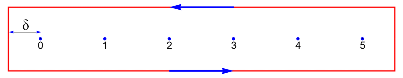
Figure 2: Rectangular contour $C$ of integration for the right hand side of (7) for particular value $k=5$ encircling points $0,1,...,5$. This shape is especially well suited for numerical investigations.

However, before applying the above Lemma it is convenient to make several elementary transformations in (5).

$$a_{k} =\gamma+{\displaystyle\sum\limits_{j=1}^{k}}\left(-1\right)^{j}\binom{k}{j}\varphi(1+j\varepsilon)=$$

$$=\gamma+{\displaystyle\sum\limits_{j=1}^{k}}\left(-1\right)^{j}\binom{k}{j}\zeta(1+j\varepsilon)-\frac{1}{\varepsilon}{\displaystyle\sum\limits_{j=1}^{k}}\frac{\left(-1\right)^{j}}{j}\binom{k}{j}$$

The last sum is

$${\displaystyle\sum\limits_{j=1}^{k}}\frac{\left(-1\right)^{j}}{j}\binom{k}{j}=-\gamma-\psi^{(0)}(k+1)=-H_{k}$$

where $\psi^{(0)}(s)$ is the polygamma function and $H_{k}\equiv\sum_{i=1}^{k}1/i$ is the $k^{\text{th}}$ harmonic number. Finally we get:

$$a_{k}=\gamma+\frac{H_{k}}{\varepsilon}+{\displaystyle\sum\limits_{j=1}^{k}}\left(-1\right)^{j}\binom{k}{j}\zeta(1+j\varepsilon)$$ (8)

Now choosing the rectangular contour of integration (Figure 1) and applying the above Lemma (7) to (5) we get:

$$a_{k}=\frac{\left(-1\right)^{k}k!}{2\pi i}\left({\displaystyle\int\limits_{-\delta+i\delta}^{-\delta-i\delta}}f_{k}ds+{\displaystyle\int\limits_{-\delta-i\delta}^{k+\delta-i\delta}}f_{k}ds+{\displaystyle\int\limits_{k+\delta-i\delta}^{k+\delta+i\delta}}f_{k}ds+{\displaystyle\int\limits_{k+\delta+i\delta}^{-\delta+i\delta}}f_{k}ds\right)$$ (9)

where the integrand is:

$$f_{k}\equiv f_{k}(s,\varepsilon)=\frac{\varphi(1+s\varepsilon)}{{\displaystyle\prod\limits_{i=0}^{k}}(s-i)}$$

and $\varphi$ is the regularized zeta function (4) and $\delta$ is positive parameter. (Typically $\delta=\frac{1}{2}$, see Fig. 2.)

Deforming the rectangular contour of integration to a vertical line $\operatorname{Re}s=\frac{1}{2}$ and a large semicircle on the right and performing the integral along vertical line only, that is neglecting contribution from the large semicircle, which tends to zero, we get:

$$a_{k}=\frac{\left(-1\right)^{k}k!}{2\pi i}{\displaystyle\int\limits_{+\frac{1}{2}+i\infty}^{+\frac{1}{2}-i\infty}}f_{k}(s,\varepsilon)ds$$

After applying functional equation for the Riemann zeta function (see e.g. [1], p. 12-16):

$$\zeta(1+s\varepsilon)=\pi^{\frac{1}{2}+s\varepsilon}\frac{\Gamma(-\frac{s\varepsilon}{2})}{\Gamma(\frac{1+s\varepsilon}{2})}\zeta(-s\varepsilon)$$ (10)

we get

$$a_{k}=\gamma+\frac{H_{k}}{\varepsilon}+\frac{\left(-1\right)^{k}k!}{2\pi i}{\displaystyle\int\limits_{+\frac{1}{2}+i\infty}^{+\frac{1}{2}-i\infty}}\frac{\pi^{\frac{1}{2}+s\varepsilon}\frac{\Gamma(-\frac{s\varepsilon}{2})}{\Gamma(\frac{1+s\varepsilon}{2})}\zeta(-s\varepsilon)}{{\displaystyle\prod\limits_{i=0}^{k}}(s-i)}ds$$

Performing change of variable $s\rightarrow-s$ yields:

$$a_{k}=\gamma+\frac{H_{k}}{\varepsilon}-\frac{\left(-1\right)^{k}k!}{2\pi i}{\displaystyle\int\limits_{-\frac{1}{2}-i\infty}^{-\frac{1}{2}+i\infty}}\frac{\pi^{\frac{1}{2}-s\varepsilon}\frac{\Gamma(\frac{s\varepsilon}{2})}{\Gamma(\frac{1-s\varepsilon}{2})}\zeta(s\varepsilon)}{{\displaystyle\prod\limits_{i=0}^{k}}(-s-i)}ds$$

Using elementary identity valid for integer $k$:

$${\displaystyle\prod\limits_{i=0}^{k}}(-s-i)=-\left(-1\right)^{k}{\displaystyle\prod\limits_{i=0}^{k}}(s+i)$$

and converting the product on the right into the Pochhammer symbol usually denoted $(s)_{n}$:

$${\displaystyle\prod\limits_{i=0}^{k}}(s+i)=\frac{\Gamma\left(s+k+1\right)}{\Gamma\left(s\right)}\equiv(s)_{k+1}$$

we get:

$$a_{k}=\gamma+\frac{H_{k}}{\varepsilon}+\frac{k!}{2\pi i}{\displaystyle\int\limits_{-\frac{1}{2}-i\infty}^{-\frac{1}{2}+i\infty}}\pi^{\frac{1}{2}-s\varepsilon}\frac{\Gamma(\frac{s\varepsilon}{2})}{\Gamma(\frac{1-s\varepsilon}{2})}\frac{\Gamma\left(s\right)}{\Gamma\left(s+k+1\right)}\zeta(s\varepsilon)ds$$

Now defining the integrand as:

$$f_{k}(s,\varepsilon)=\pi^{\frac{1}{2}-s\varepsilon}\frac{\Gamma(\frac{s\varepsilon}{2})}{\Gamma(\frac{1-s\varepsilon}{2})}\frac{\Gamma\left(s\right)}{\Gamma\left(s+k+1\right)}\zeta(s\varepsilon)$$ (11)

we get

$$a_{k} =\gamma+\frac{H_{k}}{\varepsilon}+\frac{k!}{2\pi i}{\displaystyle\int\limits_{-\frac{1}{2}-i\infty}^{-\frac{1}{2}+i\infty}}f_{k}(s,\varepsilon)ds=$$ (12)

$$=\gamma+\frac{H_{k}}{\varepsilon}+\frac{k!}{2\pi i}\left({\displaystyle\int\limits_{+\frac{1}{2}-i\infty}^{+\frac{1}{2}+i\infty}}f_{k}(s,\varepsilon)ds-2\pi i\;\text{Res}\left(f_{k}(s,\varepsilon),0\right)\right)$$ (13)

We can finally move the line of integration from $\operatorname{Re}s=-\frac{1}{2}$ to $\operatorname{Re}s=+\frac{1}{2}$ and subtract the contribution from residue of the integrand in $s=0$. It turns out that this residue is:

$$\frac{\gamma\varepsilon+H_{k}}{\varepsilon k!}$$ (14)

which miraculously cancels exactly the first and the second term in (12)

$$a_{k}=\frac{k!}{2\pi i}{\displaystyle\int\limits_{+\frac{1}{2}-i\infty}^{+\frac{1}{2}+i\infty}}f_{k}(s,\varepsilon)ds$$ (15)

It is convenient to introduce the following notation:

$$g_{k}(s,\varepsilon) \equiv\pi^{\frac{1}{2}-s\varepsilon}\frac{\Gamma(\frac{s\varepsilon}{2})}{\Gamma(\frac{1-s\varepsilon}{2})}\frac{\Gamma\left(s\right)}{\Gamma\left(s+k+1\right)}$$ (16)

$$f_{k}(s,\varepsilon) =g_{k}(s,\varepsilon)\zeta(s\varepsilon)$$

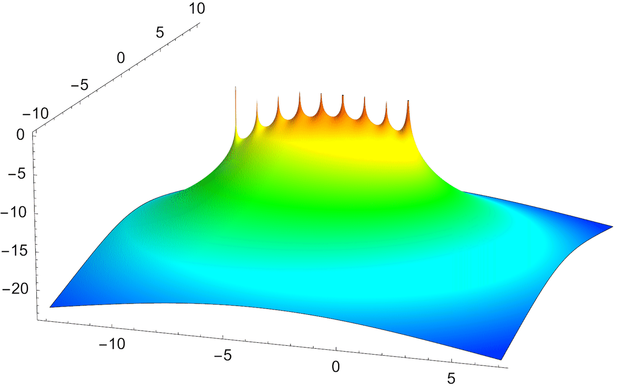
Figure 3: Absolute value of the integrand (16) for $k=8$ and $\varepsilon=2^{-5}$. Vertical scale is logarithmic for better visualisation. The right half-plane of complex variable $s$ is free of singularities. Simple poles in $s=0,-1,-2,...,-k$ due to factor $\Gamma(s)$ in (16) are visible.

The integrand in (16) has several remarkable features. It is free of singularities in the right half-plane and decays there exponentially to zero. Hence, the vertical line of integration may be freely moved to the right without any change of the integral. Therefore the integral is well-suited for applying the saddle point method. Let us now remind the following important result (see [2] for a very accessible presentation of this method):

Theorem 2

The saddle-point method (or: Method of steepest descent). An integral depending of some real parameter $\lambda$ may be approximated for large value of this parameter as

$$\int\tau(x)e^{\lambda\omega(x)}dx\sim\tau(x_{0})e^{\lambda\omega(x_{0})}\sqrt{-\frac{2\pi}{\lambda\omega^{\prime\prime}(x_{0})}},\quad\omega^{\prime}(x_{0})=0$$ (17)

(The solution $x_{0}$ of the equation $\omega^{\prime}(x_{0})=0$ is the saddle point.)

In our case the discrete index $k$ plays the role of parameter $\lambda$ although it is not just multiplying factor. It is evident that in order to apply the above theorem to integral (16) one has to choose $\tau\equiv 1$ and $\omega=\log\left(f_{k}(s,\varepsilon)\right)$. More precisely:

$$\omega_{k}(s,\varepsilon)\equiv\log\left(f_{k}(s,\varepsilon)\right)$$ (18)

All the computations below are elementary but very tedious, so they were performed and checked with the help of Wolfram Mathematica [15].

We shall also need the first and the second derivative of the integrand (16) with respect to complex variable $s$. Having these we can compute derivatives of $\omega_{k}(s,\varepsilon)$ as:

$$\frac{\partial}{\partial s}\omega_{k}(s,\varepsilon)=\frac{\frac{\partial}{\partial s}f_{k}(s,\varepsilon)}{f_{k}(s,\varepsilon)}\equiv\frac{f_{k}^{(1)}(s,\varepsilon)}{f_{k}(s,\varepsilon)}$$ (19)

$$\frac{\partial^{2}}{\partial s^{2}}\omega_{k}(s,\varepsilon)=\frac{\frac{\partial^{2}}{\partial s^{2}}f_{k}(s,\varepsilon)}{f_{k}(s,\varepsilon)}-\left(\frac{\frac{\partial}{\partial s}f_{k}(s,\varepsilon)}{f_{k}(s,\varepsilon)}\right)^{2}\equiv\frac{f_{k}^{(2)}(s,\varepsilon)}{f_{k}(s,\varepsilon)}-\left(\frac{f_{k}^{(1)}(s,\varepsilon)}{f_{k}(s,\varepsilon)}\right)^{2}$$ (20)

Let $\psi(s)$ and $\psi^{(1)}(s)$ denote digamma function and its first derivative, respectively. Introducing the following denotations:

$$p_{k}(s,\varepsilon)\equiv\psi(s)-\psi(s+k+1)+\frac{\varepsilon}{2}\left(\psi\left(\frac{s\varepsilon}{2}\right)+\psi\left(\frac{1-s\varepsilon}{2}\right)-2\log(\pi)\right)$$

$$p_{k}^{(1)}(s,\varepsilon)\equiv\psi^{(1)}(s)-\psi^{(1)}(s+k+1)+\left(\frac{\varepsilon}{2}\right)^{2}\left(\psi^{(1)}\left(\frac{s\varepsilon}{2}\right)-\psi^{(1)}\left(\frac{1-s\varepsilon}{2}\right)\right)$$

after some elementary but tedious computations we get:

$$f_{k}^{(1)}(s,\varepsilon)\equiv\frac{\partial}{\partial s}f_{k}(s,\varepsilon)=g_{k}(s,\varepsilon)\left(p_{k}(s,\varepsilon)\zeta\left(\varepsilon s\right)+\varepsilon\zeta^{\prime}\left(\varepsilon s\right)\right)$$ (21)

In a similar way we can obtain the second derivative of $f_{k}(s,\varepsilon)$. Introducing denotations:

$$q_{k}(s,\varepsilon)\equiv p_{k}(s,\varepsilon)^{2}+p_{k}^{(1)}(s,\varepsilon)$$

$$q_{k}^{(1)}(s,\varepsilon)\equiv 2\varepsilon p_{k}(s,\varepsilon)$$

we get:

$$f_{k}^{(2)}(s,\varepsilon)\equiv\frac{\partial^{2}}{\partial s^{2}}f_{k}(s,\varepsilon)=g_{k}(s,\varepsilon)\left(q_{k}(s,\varepsilon)\zeta\left(\varepsilon s\right)+q_{k}^{(1)}(s,\varepsilon)\zeta^{\prime}\left(\varepsilon s\right)+\varepsilon^{2}\zeta^{{}^{\prime\prime}}\left(\varepsilon s\right)\right)$$ (22)

Inserting (21) and (22) into (19) and (20) we get:

$$\frac{\partial}{\partial s}\omega_{k}(s,\varepsilon)=p_{k}(s,\varepsilon)-\frac{\pi\varepsilon}{2}\tan\left(\frac{\pi s\varepsilon}{2}\right)+\varepsilon\frac{\zeta^{{}^{\prime}}\left(\varepsilon s\right)}{\zeta\left(\varepsilon s\right)}$$ (23)

$$\frac{\partial^{2}}{\partial s^{2}}\omega_{k}(s,\varepsilon)=q_{k}(s,\varepsilon)-\left(\frac{\pi\varepsilon}{2}\tan\left(\frac{\pi s\varepsilon}{2}\right)\right)^{2}+\varepsilon^{2}\left(\frac{\zeta^{{}^{{}^{\prime\prime}}}\left(\varepsilon s\right)}{\zeta\left(\varepsilon s\right)}-\left(\frac{\zeta^{{}^{\prime}}\left(\varepsilon s\right)}{\zeta\left(\varepsilon s\right)}\right)^{2}\right)$$ (24)

Having explicitly calculated derivatives of the integrand we are ready to apply the saddle point method (17). First we have to find the location of saddle points. Equating (21) or (23) to zero gives:

$$p_{k}(s,\varepsilon)\zeta\left(\varepsilon s\right)+\varepsilon\zeta^{\prime}\left(\varepsilon s\right)=0$$ (25)

Note that for variable $s$ having large imaginary part we have (cf. e.g. [5], formula (20)):

$$\zeta\left(s\right) \sim 1$$ (26)

$$\zeta^{{}^{\prime}}\left(s\right) \sim 0$$

$$\zeta^{{}^{{}^{\prime\prime}}}\left(s\right) \sim 0$$

The above approximations seem very radical and illegitimate, because the zeta function seems to disappear from the reasoning at this stage. Nevertheless, they are satisfied with accuracy to many significant digits along the integration path which, let us recall, can be shifted arbitrarily far to the right. After all, the zeta is present there, at least by its functional equation (10), which has been used above.

Therefore, instead of (25), we simply get:

$$3+2k+s\varepsilon\left(2\ln\frac{2\pi}{s\varepsilon}\pm i\pi\right)=0$$ (27)

(One has to be careful with logarithms of complex arguments so as not to ignore a case and therefore not miss a solution.) Equation (27) may be solved explicitly with respect to $s$ giving the complex location of $k^{\text{th}}$ saddle point (for a given small parameter $\varepsilon$):

$$s_{k}=\frac{k+\frac{3}{2}}{\varepsilon W\left(\pm\frac{k+\frac{3}{2}}{2\pi i}\right)}$$ (28)

where $W$ is the Lambert function satisfying transcendental functional equation:

$$s=W(s)e^{W(s)}$$

Incidentally, formula (28) resembles approximate formula for the imaginary parts $y_{n}$ of complex zeta zeros found by André LeClair (see [8], formula (22)):

$$y_{n}=\frac{n-\frac{11}{8}}{W\left(\frac{n-\frac{11}{8}}{e}\right)}$$

From (28) it is evident that distribution of saddle points on the complex plane scales as the inverse of parameter $\varepsilon$.

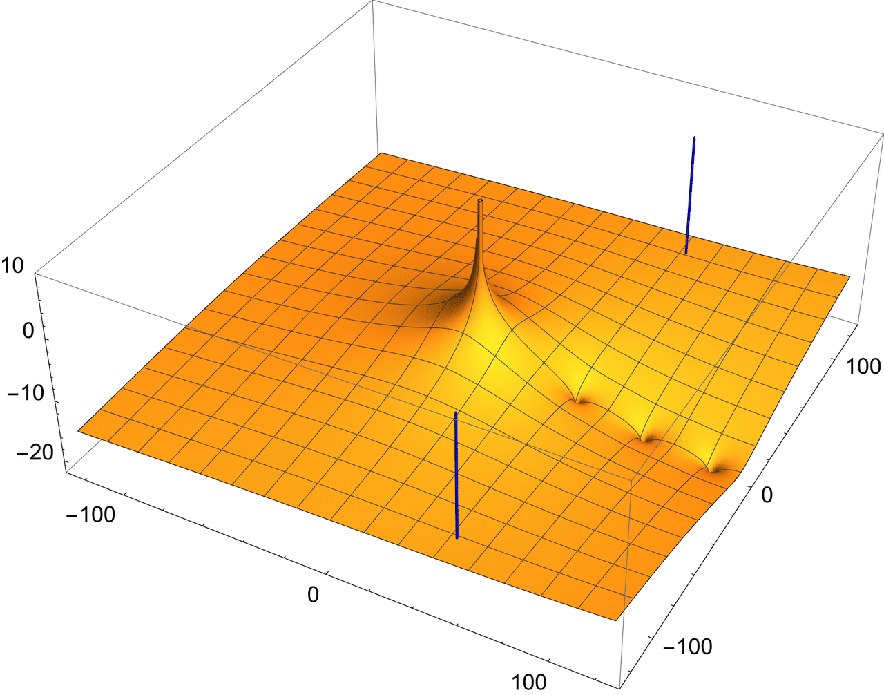
Figure 4: The logarithm of the absolute value of the integrand (11) for $k=2$ and $\varepsilon=2^{-4}$. Positions of saddle points is marked by vertical lines. The saddle nature of these points is practically invisible due to the scale of the figure. Also, three singularities for $s=0,-1,-2$ merged into single peak. Better visualisation is presented on the next Figure 5.

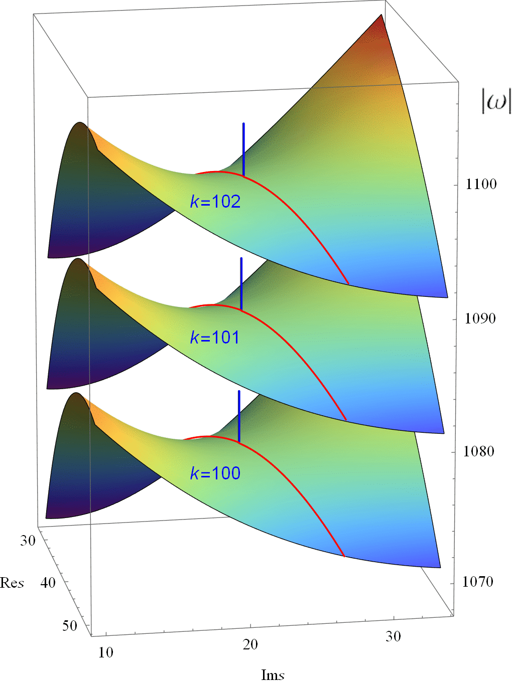
Figure 5: Typical family of fragments of absolute values of the function $\omega_{k}(s,\varepsilon)$ (18) in the vicinity of saddle points for $k=100,101$ and $102$. Blue vertical segments mark the position of the saddles. The red lines are the curves of the steepest descent.

4 Completion of computations

Having calculated the second derivative of the integrand and the positions of the stationary points, we can finally use the theorem (17) and provide an asymptotic expression for $a_{k}$:

$$a_{k}(\varepsilon)\simeq-\operatorname{Re}\left(\frac{k!}{\pi i}\sqrt{\frac{2\pi}{-\frac{\partial^{2}}{\partial s^{2}}\omega_{k}(s_{k},\varepsilon)}}f_{k}(s_{k},\varepsilon)\right)$$ (29)

To get the sought asymptotic formula for $\gamma_{n}$ coefficients, all that remains is to insert (29) into the general expression (6) and make some elementary approximations. (As always, Mathematica procedures such as Limit, Series, etc. save a lot of time and effort while ensuring that the results are error free.) In particular:

$$\frac{\partial^{2}}{\partial s^{2}}\omega_{k}(s_{k},\varepsilon)\simeq\frac{3+2k}{2s^{2}}+\frac{\varepsilon}{s}-\frac{\pi^{2}\varepsilon^{2}}{4}\left(1+\tan\left(\frac{\pi s\varepsilon}{2}\right)^{2}\right)$$ (30)

Using (26) we can also put:

$$f_{k}(s,\varepsilon)\simeq g_{k}(s,\varepsilon)$$ (31)

Remembering that for large imaginary part of $s$

$$\Gamma(s) \simeq\sqrt{\frac{2\pi}{s}}e^{-s}s^{s}$$

$$\cos(s) \simeq\frac{e^{-is}}{2}$$

we have:

$$g_{k}(s,\varepsilon)\simeq\frac{1}{2}\pi^{\frac{1}{2}-s\varepsilon}s^{-k-2}\left(2s-k-k^{2}\right)\frac{\Gamma(\frac{s\varepsilon}{2})}{\Gamma(\frac{1-s\varepsilon}{2})}$$ (32)

It is clear that, since finally $\varepsilon$ tends to zero, it is sufficient to take only the first term in (6)

$$\gamma_{n}\simeq\frac{a_{k}(\varepsilon)}{\varepsilon^{n}}\quad\quad\varepsilon\rightarrow 0$$ (33)

Inserting to (33) expression for $a_{k}(\varepsilon)$ (29) together with (30), (31) and (32) we finally get:

$$\gamma_{n}\sim\sqrt{\frac{2}{\pi}}n!\operatorname{Re}\frac{\Gamma\left(s_{n}\right)e^{-cs_{n}}}{\left(s_{n}\right)^{n}\sqrt{n+s_{n}+\frac{3}{2}}}$$

(In fact, there is always a pair of mutually conjugate saddles but contributions due to their imaginary parts cancels.)

It is probably quite astonishing that after making so many approximations the final formula for $\gamma_{n}$ works so well as computer experiments show convincingly. As expected, in this formula there is no longer the auxiliary parameter $\varepsilon$, which fulfilled its important but temporary role in numerical computations (with the help of formula (6)), and finally simply get shortened.

5 Summary of results

Let’s collect the final results. Let $c$ be a complex constant:

$$c=\log(2\pi)+\frac{\pi}{2}i=\log(2\pi i)$$

Now asymptotics of Stieltjes constants when $n\rightarrow\infty$ (in practice it suffices that $n\gg 0$) is:

$$\gamma_{n}\sim\sqrt{\frac{2}{\pi}}n!\operatorname{Re}\frac{\Gamma\left(s_{n}\right)e^{-cs_{n}}}{\left(s_{n}\right)^{n}\sqrt{n+s_{n}+\frac{3}{2}}}$$ (34)

where complex saddle points are (note that now there is no $\varepsilon$ which get shortened):

$$s_{n}=\frac{n+\frac{3}{2}}{W\left(\pm\frac{n+\frac{3}{2}}{2\pi i}\right)}$$ (35)

The $250$ initial values of the complex saddles (35) are shown in the Figure 6. Very good agreement of approximated values calculated using (34) with actual values of $\gamma_{n}$ is shown in Figure 7.

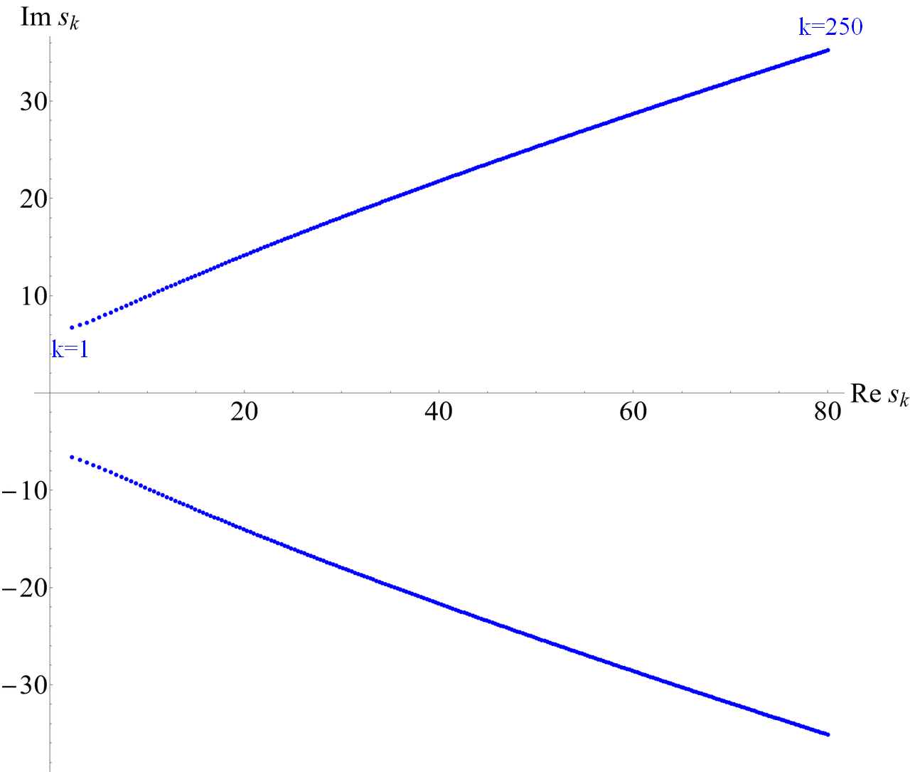
Figure 6: Distribution of 250 initial saddle points on the complex plane. There are two symmetrical branches, the lower one is the complex conjugate of the upper one.

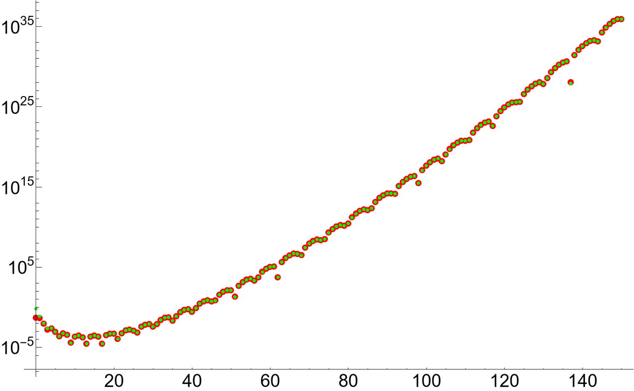
Figure 7: Comparison of absolute values of actual Stieltjes coefficients (green dots) with those calculated from asymptotic formula (34) (red dots) shows good agreement (except $\gamma_{0}$), even for that ”unruly” value $n=137$.

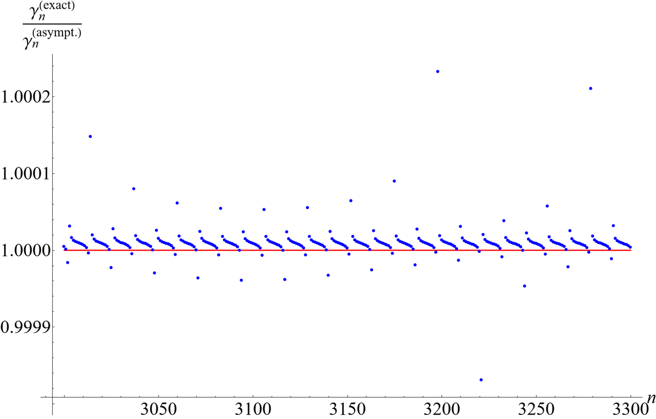
Figure 8: Unfortunately, the good impression after looking at Figure 7 diminishes a bit when we look at the graph of the ratio of the exact $\gamma_{n}$ values to the asymptotic values (34) for example in the range of $n=3000-3300$. Although this ratio is very close to one, with an accuracy generally better than $10^{-4}$, there are distinct, periodic structures: points are arranged on certain curves resembling the family of cotangent functions. But it is in these structures that the essence of Riemann’s zeta is contained, including the Riemann hypothesis, i.e. what was rejected when the approximations (26) were made. Also note, which is somewhat surprising, that the blue points lie slightly above the red straight line that represents the value of one. But, as the saying goes, when one door shuts, another one opens. And indeed: this result opens up a whole new field for very fruitful research on the Stieltjes constants, which will be the subject of the next publication.

6 Application: Signs of $\gamma_{n}$

As a by-product of these intricate computations, we can get a compact expression for the signs of the Stieltjes constants. Formula (34) hides the characteristic behavior of Stieltjes constants when $n$ grows, that is large and growing oscillations with diminishing frequency superimposed on the strongly growing trend. This behavior may be demonstrated as follows. Recall higher order Stirling formula for $\Gamma(x)$:

$$\Gamma(x)\simeq\frac{1}{6}\sqrt{\frac{\pi}{2}}e^{-x}x^{x-\frac{3}{2}}(12x+1)$$

Applying it to $\Gamma\left(s_{n}\right)$ in (34) we get:

$$\gamma_{n}\simeq 2n!\operatorname{Re}\frac{\left(s_{n}\right)^{s_{n}-n-\frac{3}{2}}(s_{n}+\frac{1}{12})e^{-(c+1)s_{n}}}{\sqrt{n+s_{n}+\frac{3}{2}}}$$ (36)

For $n\gg 1$ fractions $\frac{1}{12}$ and $\frac{3}{2}$ under the square root may be neglected since $s_{n}$ grows fast with $n$:

$$\gamma_{n} \simeq 2n!\operatorname{Re}\frac{\left(s_{n}\right)^{s_{n}-n-\frac{1}{2}}e^{-(c+1)s_{n}}}{\sqrt{n+s_{n}}}=$$

$$=2n!\operatorname{Re}\frac{\exp\left[(s_{n}-n-\frac{1}{2})\ln\left(s_{n}\right)\right]e^{-(c+1)s_{n}}}{\exp\left[\frac{1}{2}\ln\left(n+s_{n}\right)\right]}=$$

$$=2n!\operatorname{Re}\exp\left[(s_{n}-n-\frac{1}{2})\ln\left(s_{n}\right)-\frac{1}{2}\ln\left(n+s_{n}\right)-(c+1)s_{n}\right]$$

Applying once again Stirling formula to $n!$ we have:

$$\gamma_{n}\simeq\sqrt{8\pi}\operatorname{Re}\exp\left[\frac{1}{2}\ln(n)+n\left(\ln(n)-1\right)+(s_{n}-n-\frac{1}{2})\ln\left(s_{n}\right)-\frac{1}{2}\ln\left(n+s_{n}\right)-(c+1)s_{n}\right]$$ (37)

Introducing finally complex ”phase” as:

$$\varphi_{n}\equiv\frac{1}{2}\ln(8\pi)-n+(n+\frac{1}{2})\ln(n)+(s_{n}-n-\frac{1}{2})\ln\left(s_{n}\right)-\frac{1}{2}\ln\left(n+s_{n}\right)-(c+1)s_{n}$$ (38)

we get particularly simple expression:

$$\gamma_{n}\simeq\operatorname{Re}\left[e^{\varphi_{n}}\right]=e^{\operatorname{Re}\varphi_{n}}\cos\left(\operatorname{Im}\varphi_{n}\right)$$ (39)

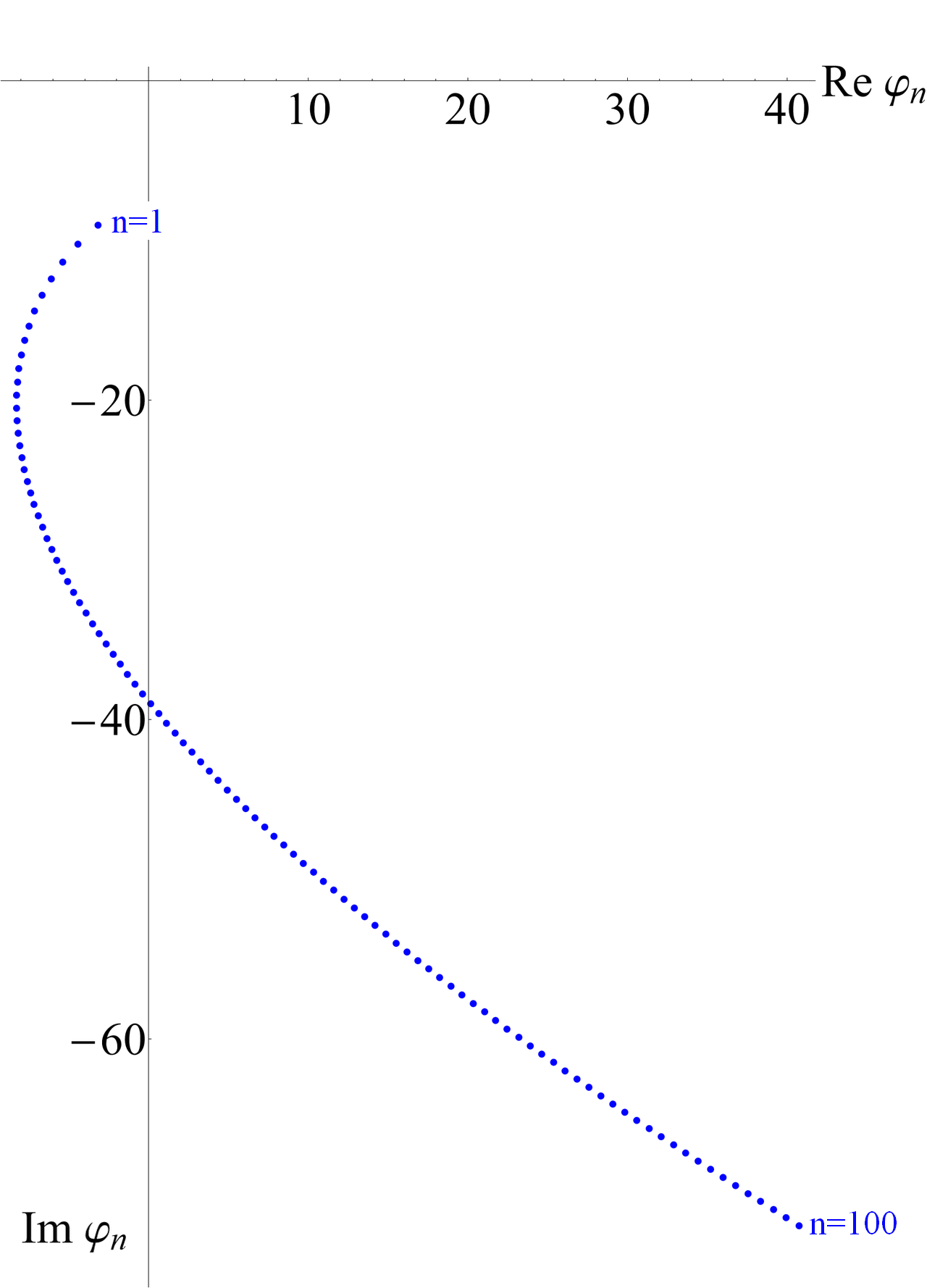
Figure 9: Distribution of complex values of phase $\varphi_{n}$ given by (38) for $n=1,2,...,100$. It is clear that thay lie along certain smooth curve. It is also obvious that the exponent of the real part of the phase (38) controls the rapid growth of $\gamma_{n}$, while the cosine of the imaginary part of the phase is responsible for the oscillations of decreasing frequency.

Formula (39) gives almost as good approximation as (34) but it shows in a manifest way mentioned above basic properties of $\gamma_{n}$ (trend and oscillations). It is then clear that the statement quoted at the beginning that ”Stieltjes constants […] change signs in a complex pattern” [14] is not true. In particular, one can quickly calculate sign of $\gamma_{n}$, even for extremely high $n$, since it is obviously equal to the sign of $\cos\left(\operatorname{Im}\varphi_{n}\right)$ and the phase (38) can be computed effectively for $n$ at least up to $10^{1,000,000}$. (See [9] for extensive computations of signs of Stieltjes constants using the above formulas.) For example:

$n$	sign of $\gamma_{n}$
$10^{10}$	$+1$
$10^{100}$	$+1$
$10^{1000}$	$+1$
$10^{10\,000}$	$-1$
$10^{100\,000}$	$-1$
$10^{1,000\,000}$	$+1$

7 Appendix - samples of Mathematica notebooks

As mentioned in the main text, Wolfram’s Mathematica [15] made very tedious and convoluted computations much easier and ensured that there were no mistakes in them. This program was used very intensively – for symbolic transformations and in terms of its enormous purely numerical capabilities and finally for its rich graphical presentations of the obtained results. Figure 9 is an example of how well Mathematica is doing to check that the contour integral (9) is indeed equal to the binomial alternating sum (8). I cannot imagine how to verify this fact with such high precision without computer support. Another example: Figure 10 shows how Mathematica solves the transcendental equations (27).

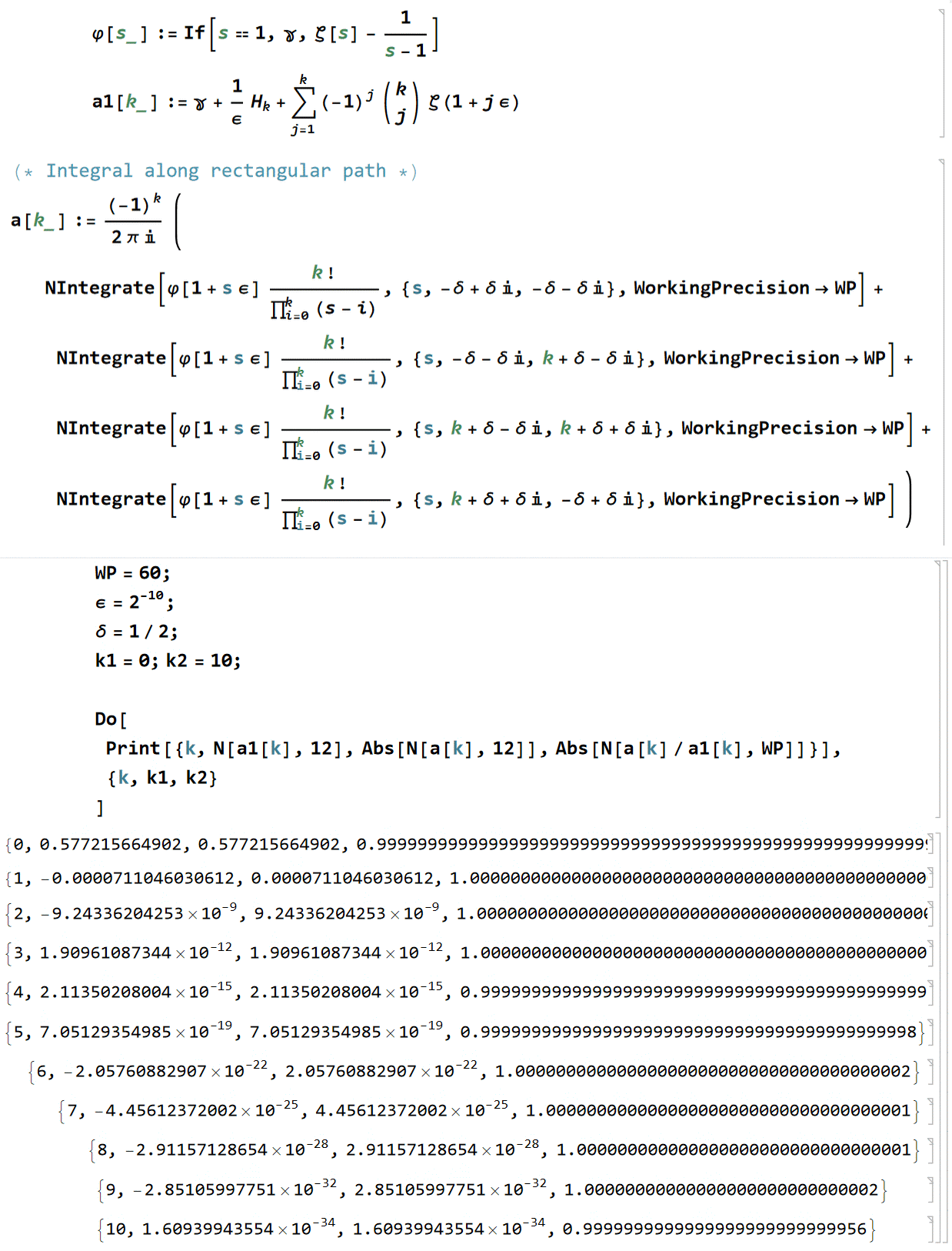
Figure 10: Checking the Nørlund-Rice formula (7) using Mathematica.

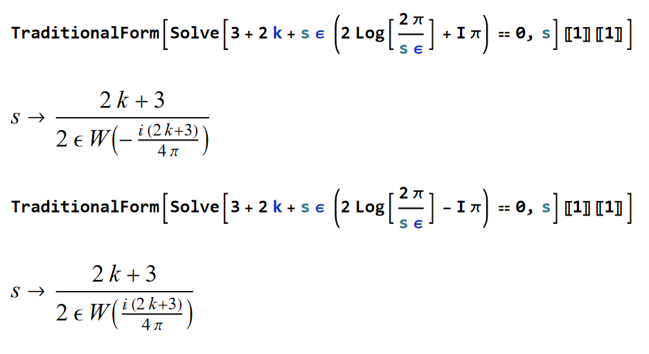
Figure 11: Illustration of the Solve procedure capabilities applied to equations (27).

References

- [1] Harold M. Edwards, Riemann’s Zeta Function, Dover Publications, 2001.
- [2] Arthur Erdélyi, Asymptotic Expansions, Dover Publications, 1956.
- [3] Lazhar Fekih-Ahmed, A New Effective Asymptotic Formula for the Stieltjes Constants, https://arxiv.org/abs/1407.5567v3 2014.
- [4] Philippe Flajolet and Robert Sedgewick, Mellin transforms and asymptotics: Finite differences and Rice’s integrals, Theoretical Computer Science 144 (1995) p. 101–124.
- [5] Philippe Flajolet and Linas Vepstas, On Differences of Zeta Values, arXiv:math/0611332v2 [math.CA]
- [6] Charles Knessl and Mark W. Coffey, An Effective Asymptotic Formula for the Stieltjes Constants, Mathematics of Computation, Vol. 80, Nr 273, January 2011, p. 379–386.
- [7] Donald E. Knuth, The Art of Computer Programming, vol. 3: Sorting and Searching, second ed., Addision-Wesley, Reading, MA, 1998.
- [8] André LeClair, An electrostatic depiction of the validity of the Riemann Hypothesis and a formula for the N-th zero at large N, https://arxiv.org/abs/1305.2613v5.
- [9] Artur Jasiński, https://oeis.org/A114523; https://oeis.org/A114524 in: Neil Sloan, The On-Line Encyclopedia of Integer Sequences, http://oeis.org/
- [10] Krzysztof Maślanka and Andrzej Koleżyński. The High Precision Numerical Calculation of Stieltjes Constants. Simple and Fast Algorithm, Computational Methods in Science and Technology, Volume 28 (2) 2022, 47–59; on-line version available at: https://cmst.eu/articles/the-high-precision-numerical-calculation-of-stieltjes-constants-simple-and-fast-algorithm/
- [11] Krzysztof Maślanka and Marek Wolf, Are the Stieltjes constants irrational? Some computer experiments, Computational Methods in Science and Technology, Volume 26 (3) 2020, p. 77–87; on-line version available at: https://cmst.eu/articles/are-the-stieltjes-constants-irrational-some-computer-experiments/
- [12] Niels Erik Nørlund, Vorlesungen über Differenzenrechnung, 1924, Springer, Berlin; reprinted: 1954, Chelsea Publishing Company, New York.
- [13] Richard Bruce Paris, An Asymptotic Expansion for the Stieltjes Constants, Mathematica Aeterna, Vol. 5, 2015, no. 5, p. 707 - 716.
- [14] https://en.wikipedia.org/wiki/Stieltjes_constants
- [15] Wolfram Research, Inc., Mathematica, Version 13.1, Champaign, Illinois (2022).
- [16] https://mathworld.wolfram.com/LambertW-Function.html
- [17] https://mathworld.wolfram.com/StirlingNumberoftheFirstKind.html