Forces are not Enough: Benchmark and Critical Evaluation for Machine Learning Force Fields with Molecular Simulations

Abstract

Molecular dynamics (MD) simulation techniques are widely used for various natural science applications. Increasingly, machine learning (ML) force field (FF) models begin to replace ab-initio simulations by predicting forces directly from atomic structures. Despite significant progress in this area, such techniques are primarily benchmarked by their force/energy prediction errors, even though the practical use case would be to produce realistic MD trajectories. We aim to fill this gap by introducing a novel benchmark suite for learned MD simulation. We curate representative MD systems, including water, organic molecules, peptide, and materials, and design evaluation metrics corresponding to the scientific objectives of respective systems. We benchmark a collection of state-of-the-art (SOTA) ML FF models and illustrate, in particular, how the commonly benchmarked force accuracy is not well aligned with relevant simulation metrics. We demonstrate when and how selected SOTA methods fail, along with offering directions for further improvement. Specifically, we identify stability as a key metric for ML models to improve. Our benchmark suite comes with a comprehensive open-source codebase for training and simulation with ML FFs to facilitate future work.

1 Introduction

Molecular Dynamics (MD) simulation is a widely used technique that provides atomistic insights into physical phenomena in materials and biological systems (Alder & Wainwright, 1959; Rahman, 1964; Schlick, 2010). MD simulations use force fields (FFs) to characterize the underlying potential energy surface (PES) of the system and simulate long trajectories based on Newton’s second law (Frenkel & Smit, 2001). The PES itself is challenging to compute and would ideally be done through quantum chemistry which is computationally expensive. Traditionally, the alternative has been parameterized force fields built from empirically chosen functional forms (Halgren, 1996). Recently, machine learning (ML) force fields (Unke et al., 2021b) have shown promise to accelerate MD simulations by orders of magnitude while being quantum chemically accurate. The learned force field can then simulate MD or perform structural relaxation. However, despite MD simulations being a primary motivation for ML FFs, the evidence supporting the utility of ML FFs is often based on their accuracy in reconstituting forces across test cases (Faber et al., 2017) without involving simulations. This paper highlights the importance of simulation-based evaluation, demonstrating that force accuracy alone does not suffice for effective simulation (Figure 1 (a)).

Figure 1: (a) Results on simulating a water system with ML force fields. Models are sorted by force mean absolute error (MAE) in descending order. High stability and low radial distribution function (RDF) MAE are better. Performance in force error does not align with simulation-based metrics. (b) Force-only evaluation may not reveal key factors in simulating MD with a ML force fields. In this toy example, model 2 (green) has a lower force error but likely leads to unstable simulations due to extreme forces from local pathological behavior. (c) Illustrations of MD observables.

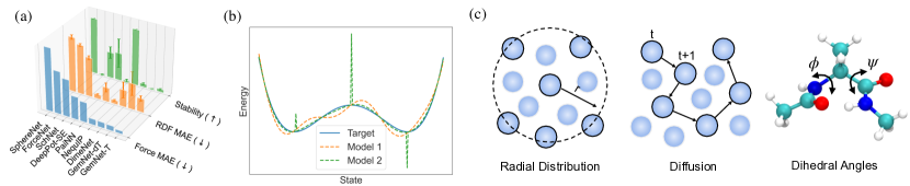
In practice, the exact recovery of the trajectories given the initial conditions is not the ultimate goal of learning MD simulations. Instead, MD simulation quality is better evaluated through macroscopic observables that characterize system properties (Leach & Leach, 2001; Tuckerman, 2010). These observables are designed to be predictive of material properties such as diffusivity in electrolyte materials (Webb et al., 2015), or reveal detailed physical mechanisms, such as the folding kinetics of proteins (Lane et al., 2011; Lindorff-Larsen et al., 2011). Although these observables are critical products of MD simulations, systematic evaluations have not been sufficiently studied in the existing literature. In particular, we show that even small errors in the force field parameters can lead to catastrophic failure in long-time simulation – ML force fields may exhibit pathological behavior such as extreme force/energy predictions on states not captured by the training data, causing the simulation to become unstable or explode (toy example illustrated in Figure 1 (b)).

A benchmark for MD simulations requires mindful design over the selection of systems, the simulation protocol, and the evaluation metrics: (1) A benchmark suite should cover diverse and representative systems to reflect the various challenges in different MD applications. (2) Simulations are computationally expensive (see Table 7 in Appendix B). An ideal benchmark must balance the cost of evaluation and the system’s complexity to obtain meaningful metrics with reasonable time and computation. (3) Selected systems should be well studied in the simulation domain, and chosen metrics should be based on physical observables that characterize the system’s important degrees of freedom or geometric features to reflect practical utility. We carefully curate four representative MD systems and design simulation protocols/metrics considering all the abovementioned desiderata.

Are current state-of-the-art (SOTA) ML FFs capable of simulating a variety of MD systems? What might cause a model to fail in simulations? This paper aims to answer these questions with a novel benchmark study. The contributions of this paper include:

• We introduce a novel benchmark suite for ML MD simulation with simulation protocols and quantitative metrics. We perform extensive experiments to benchmark a collection of SOTA ML models. We provide a complete codebase for training and simulating MD with ML FFs to lower the barrier to entry and facilitate future work.

• We show that many existing models are inadequate when evaluated on simulation-based benchmarks, even when they show accurate force prediction (as shown in Figure 1).

• By performing and analyzing MD simulations, we summarize common failure modes and discuss the causes and potential solutions to motivate future research.

2 Preliminaries

Training. An ML FF aims to learn the potential energy surface $\hat{E}(\bm{x})\in\mathbb{R}$ as a function of atomic coordinates $\bm{x}\in\mathbb{R}^{N\times 3}$ ($N$ is the number of atoms), by fitting atom-wise forces $\hat{\bm{F}}(\bm{x})$ and energies from a training dataset:$\{\bm{x}_{i},\bm{F}_{i},E_{i}\}_{i=1}^{N_{\mathrm{data}}}$, where $\bm{x}_{i}\in\mathbb{R}^{N\times 3},\bm{F}\in\mathbb{R}^{N\times 3},E\in\mathbb{R}$. For evaluation, the test force/energy prediction accuracy is often used as a proxy to quantify the quality of the learned PES. The force field learning protocol has been well established (Unke et al., 2021b).

MD simulation. Simulating molecular behaviors requires integrating a Newtonian equation of motion $d^{2}\bm{x}/dt^{2}=m^{-1}\bm{F}(\bm{x})$ with forces obtained by differentiating $\hat{E}(x)$: $\bm{F}(\bm{x})=-{\partial\hat{E}(\bm{x})}/{\partial\bm{x}}$. To mimic desired thermodynamic conditions such as constant temperature/pressure, an appropriate thermostat and barostat are chosen to augment the equation of motion with extended variables. These conditions are system-dependent and task-dependent. The simulation produces a time series of positions $\{\bm{x}_{t}\in\mathbb{R}^{N\times 3}\}_{t=0}^{T}$ (and velocities), where $t$ is the temporal order index, and $T$ is the total simulation steps.

Observables. From the time series of positions (and velocities), observables $O({\bm{x}_{t}})$ can be computed to characterize the state of the system at different granularities. Under the ergodic hypothesis, the time averages of the simulation observables converge to distributional averages under the Gibbs measure (Frenkel & Smit, 2001): $\langle O\rangle=\frac{1}{T}\lim_{T\rightarrow\infty}\sum_{t}^{T}O(\bm{x}_{t})=\int d\bm{x}\;p(\bm{x})\ O(\bm{x})$, where $p(\bm{x})\propto\exp(-\frac{\hat{E}(\bm{x})}{k_{B}T})$ with $T$ as the bath temperature and $k_{B}$ as the Boltzmann constant. Calculations of such observables require the system to reach equilibrium. Simulation observables connect simulations to experimental measurements and are predictive of macroscopic properties of matter. Common observables (illustrated in Figure 1 (c)) include radial distribution functions (RDFs), virial stress tensor, mean-squared displacement (MSD), dihedral angles, etc. We propose evaluation metrics based on well-established observables in the respective types of systems (Section 5).

3 Related Work

ML force fields learn the potential energy surface (PES) from the data by applying expressive regressors such as kernel methods (Chmiela et al., 2017) and neural networks on symmetry-preserving representations of atomic environments (Behler & Parrinello, 2007; Khorshidi & Peterson, 2016; Smith et al., 2017; Artrith et al., 2017; Unke & Meuwly, 2018; Zhang et al., 2018b; a; Kovács et al., 2021; Thölke & De Fabritiis, 2021; Takamoto et al., 2022). Recently, graph neural network architectures (Gilmer et al., 2017; Schütt et al., 2017; Gasteiger et al., 2020; Liu et al., 2021) have gained popularity as they provide a systematic strategy for building many-body correlation functions to capture highly complex PES. In particular, equivariant representations have been shown powerful in representing atomic environments (Satorras et al., 2021; Thomas et al., 2018; Qiao et al., 2021; Schütt et al., 2021; Batzner et al., 2022; Gasteiger et al., 2021; Liao & Smidt, 2022; Chen & Ong, 2022; Gasteiger et al., 2022), leading to significant improvements in benchmarks such as MD17 and OC22/20. Some works presented simulation-based results (Unke et al., 2021a; Park et al., 2021; Batzner et al., 2022; Musaelian et al., 2022) but do not compare different models with simulation-based metrics.

Existing benchmarks for ML force fields (Ramakrishnan et al., 2014; Chmiela et al., 2017) mostly focus on force/energy prediction, with small molecules being the most typical systems. The catalyst-focused OC20 (Chanussot et al., 2021) and OC22 (Tran et al., 2022) benchmarks focus on structural relaxation with force computations, where force prediction is part of the evaluation metrics. The structural relaxation processes are around hundreds of steps, and the goal is to predict the final relaxed structure/energy. These tasks do not characterize system properties under a structural ensemble, which requires simulations that are millions of steps long. Several recent works (Rosenberger et al., 2021) have also studied the utility of certain ML FFs in MD simulations. In particular, Stocker et al. 2022 uses GemNet (Gasteiger et al., 2021) to simulate small molecules in the QM7-x (Hoja et al., 2021) dataset, with a focus on prediction robustness. Zhai et al. 2022 applies the DeepMD (Zhang et al., 2018a) architecture to simulate water and demonstrates its shortcoming in generalization across different phases. However, existing works focus on a single system and model, while evaluation protocols and quantitative metrics for model comparison remain subject to debate. The experimental results in past research are often presented qualitatively or as figures, which can be hard to analyze or used as a scalar metric for comparing performance of different models. As previous works are mostly motivated by specific use cases, they often lack coverage over diverse MD systems and have very different data generation processes, making it hard to disentangle the impact from the ML model and data. Since the experiments are designed for a single model, the simulation protocols in previous works are often too expensive for large-scale evaluation. Systematic benchmarks for simulation-based metrics are lacking in the existing literature, which obscures the challenges in applying ML FF for MD applications.

Figure 2: Visualization of the benchmarked systems. (a) MD17 molecules: Aspirin, Ethanol, Naphthalene, and Salicylic acid. (b) 64 water molecules. (c) 512 water molecules. (d) Alanine dipeptide. (e) LiPS.

4 Datasets

Table 1: Dataset summary. PBC stands for periodic boundary conditions. ^*Simulation of alanine dipeptide uses Metadynamics with implicit solvation.

Dataset System Type PBC #Atoms Simulation Length Objectives MD17 Small molecule ✗ 9-21 300 ps (600k steps) Interatomic distances Water liquid ✓ 192 500 ps (500k steps) RDF, Diffusivity Water-large liquid ✓ 1536 150 ps (150k steps) RDF, Diffusivity Alanine dipeptide Peptide ✗ 22 5 ns (2.5M steps)^* Dihedral angle analysis LiPS solid-state materials ✓ 83 50 ps (200k steps) RDF, Diffusivity

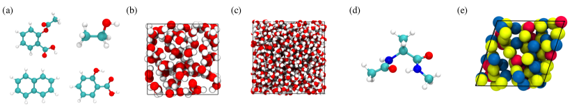
Popular benchmark datasets, such as MD17, focus on the force prediction task for gas-phase small molecules. However, successes in these tasks are not sufficient evidence for (1) capturing complex interatomic interactions that are critical for condensed phase systems; and (2) recovery of critical simulation observables that cannot be directly indicated by force prediction accuracy. This work focuses on atomic-level MD simulations that manifest complex intermolecular interactions at multiple scales. We choose systems that (1) have been frequently used in force field development (Henderson, 1974); (2) cover diverse MD applications such as materials and biology; and (3) can be simulated within reasonable time and compute. The simulation conditions such as temperature and time step sizes (Tuckerman, 2010) are configured to replicate realistic settings in MD literature. Beyond force predictions, we conduct simulations and benchmark observables that reflect the actual simulation quality, along with stability and computational efficiency. The selected systems are summarized in Table 1.

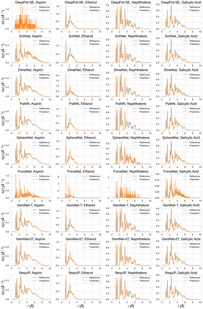
MD17 (Chmiela et al., 2017) dataset contains AIMD calculations for eight small organic molecules and is widely used as a force prediction benchmark for ML FFs. We adopt four molecules from MD17 and benchmark the simulation performance. In addition to force error, we evaluate the stability and the distribution of interatomic distances $h(r)$. For each molecule, we randomly sample 9,500 configurations for training and 500 for validation from the MD17 database. We randomly sample 10,000 configurations from the rest of the data for force error evaluation. We perform five simulations of 300 ps for each model/molecule by initializing from 5 randomly sampled testing configurations, with a time step of 0.5 fs, at 500 K temperature, under a Nosé–Hoover thermostat.

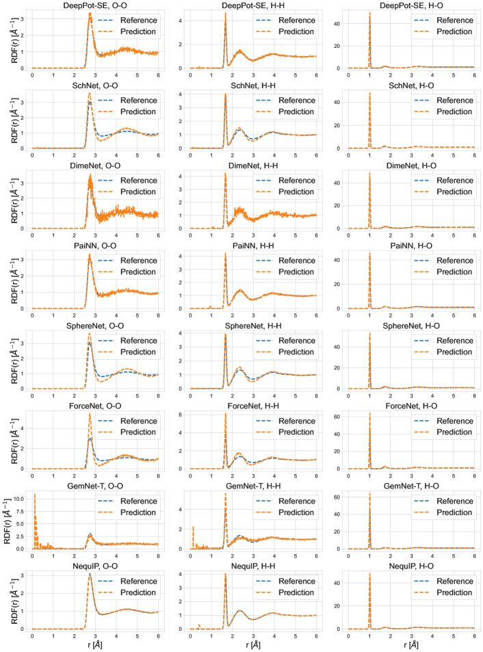
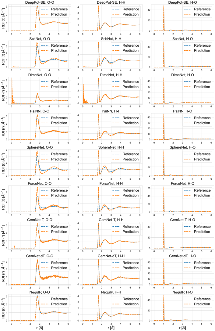
Water is arguably the most important molecular fluid in biological and chemical processes. Due to its complex thermodynamic and phase behavior, it poses great challenges for molecular simulations. In addition to force error, we evaluate simulation stability and recovery of both equilibrium statistics and dynamical statistics, namely the element-conditioned RDFs and liquid diffusion coefficient. Our dataset consists of 100,000 structures collected every 10 fs from a 1 ns trajectory sampled at equilibrium and a temperature of 300 K. We benchmarked all models with various training+validation dataset sizes (1k/10k/90k randomly sampled structures) and used the remaining 10,000 structures for testing. We performed 5 simulations of 500 ps by initializing from 5 randomly sampled testing configurations, with a time step of 1 fs, at 300 K temperature, under a Nosé–Hoover thermostat. Additionally, we evaluate model generalization to a larger system of 512 water molecules with 5 simulations of 150 ps.

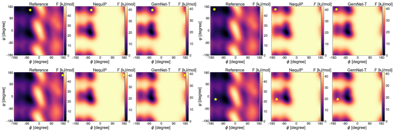
Alanine dipeptide features multiple metastable states, making it a classic benchmark for the development of MD sampling methods and force fields (Head-Gordon et al., 1989; Kaminski et al., 2001). Its geometric flexibility is well represented by the central dihedral (torsional) angles $\phi$ and $\psi$. Our reference data are obtained from simulations with explicit water molecules, with detailed protocols described in Appendix A. For faster simulation, we learn an implicitly solvated FF following a protocol similar to Chen et al. (2021). Our task is more challenging in that it aims to learn the implicitly solvated atomistic FF rather than the implicit solvation correction in Chen et al. (2021). To facilitate accelerated sampling, we apply metadynamics with $\phi$ and $\psi$ as the collective variables. We evaluate force prediction, simulation stability, and free energy surface (FES) reconstruction $F(\phi,\psi)$. Our dataset consists of 50,000 structures dumped every 2 ps from a 100 ns trajectory at a temperature of 300 K. We used 38,000 randomly sampled structures for training, 2,000 for validation, and the rest as a test set. We performed 6 simulations of 5 ns by initializing from six local minima on the FES (Figure 5) with a time step of 2 fs at 300 K, and under a Langevin thermostat to mimic random noise from solvation effects. More information on our simulation protocols can be found in Appendix A. All simulations use hydrogen bond length constraints to enable the 2 fs time step.

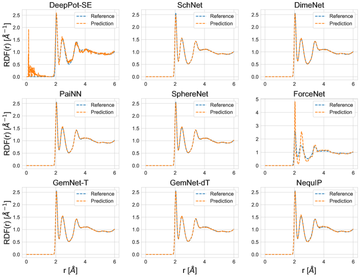
LiPS is a crystalline superionic lithium conductor relevant to battery development and a representative system for MD simulation usage in studying kinetic properties in materials. We adopt this dataset from Batzner et al. 2022, and benchmark all models on their force error, stability, RDF recovery, and Li-ion diffusivity coefficient. The dataset has 25,000 structures in total, from which we use 19,000 randomly sampled structures for training, 1,000 structures for validation, and the rest for computing force error. We conduct 5 simulations of 50 ps by initializing from 5 randomly sampled testing configurations, with a time step of 0.25 fs, at 520 K temperature, under a Nosé–Hoover thermostat.

5 Evaluation Metrics

We deisgn benchmark metrics based on physical observables that describe the most fundamental structural and dynamical properties of a MD system. These observables are relatively easy to understand and compute, and their accurate recovery is often deemed a prerequisite for computing more sophisticated observables. We note there are other observables such as thermal conductivity, viscosity, etc. of practical interest. However, these observables are often used for specific applications and require extra domain knowledge or non-standard MD set ups to compute. Our benchmark aims to simplify the MD procedure while being comprehensive, and focus on analyzing the performance of the ML models.

Distribution of interatomic distances is a low-dimensional description of the 3D structure and has been studied in previous work (Zhang et al., 2018a). For a given configuration $\bm{x}$, the distribution of interatomic distances $h(r)$ is computed with:

$$h(r)=\frac{1}{N(N-1)}\sum_{i}^{N}\sum_{j\neq=i}^{N}\delta(r-||\bm{x}_{i}-\bm{x}_{j}||)$$ (1)

where $r$ is the distance from a reference particle; $N$ is the total number of particles; $i,j$ indicates the pairs of atoms that contribute to the distance statistics; $\delta$ is the Dirac Delta function to extract value distributions. To calculate the ensemble average, $h(r)$ is calculated and averaged over frames from equilibrated trajectories. The MAE is then calculated by integrating $r$: $\mathrm{MAE_{h(r)}}=\int_{r=0}^{\infty}|\langle h(r)\rangle-\langle\hat{h}(r)\rangle|dr$, where $\langle\cdot\rangle$ is the averaging operator, $\langle\mathrm{h}(r)\rangle$ is the reference equilibrium $h(r)$, and $\langle\hat{h}(r)\rangle$ is the model-predicted equilibrium $h(r)$.

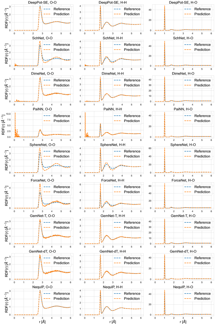
RDF. As one of the most informative simulation observables, the radial distribution function (RDF) describes the structural/thermodynamic properties of the system and is experimentally measurable (Yarnell et al., 1973; Filipponi, 1994). It has been widely used in force field development (Henderson, 1974). By definition, the RDF describes how density varies as a function of distance from a particle. For a given configuration $\bm{x}$, the RDF can be computed with the following formula:

$$\mathrm{RDF}(r)=\frac{1}{4\pi r^{2}}\frac{1}{N\rho}\sum_{i}^{N}\sum_{j\neq=i}^{N}\delta(r-||\bm{x}_{i}-\bm{x}_{j}||)$$ (2)

where $r$ is the distance from a reference particle; $N$ is the total number of particles; $i,j$ indicates the pairs of atoms that contribute to the distance statistics; $\rho$ is the density of the system; $\delta$ is the Dirac Delta function to extract value distributions. To calculate the ensemble average, $\mathrm{RDF}(r)$ is calculated and averaged over frames from equilibrated trajectories. The final RDF MAE is then calculated by integrating $r$: $\mathrm{MAE_{RDF}}=\int_{r=0}^{\infty}|\langle\mathrm{RDF}(r)\rangle-\langle\hat{\mathrm{RDF}}(r)\rangle|dr$, where $\langle\cdot\rangle$ is the averaging operator, $\langle\mathrm{RDF}(r)\rangle$ is the reference equilibrium RDF, and $\langle\hat{\mathrm{RDF}}(r)\rangle$ is the model-predicted RDF.

Diffusivity coefficient is relevant to many practical applications such as battery design (Xie et al., 2022). The diffusivity coefficient $D$ quantifies the time-correlation of the translational displacement, and can be computed from the mean square displacement:

$$D=\lim\limits_{t\to\infty}\frac{1}{6t}\frac{1}{N^{\prime}}\sum\limits_{i=1}^{N^{\prime}}|\bm{x}_{i}(t)-\bm{x}_{i}(0)|^{2}$$ (3)

where $x_{i}(t)$ is the coordinate of particle $i$ at time $t$, and $N^{\prime}$ is the number of particles being tracked in the system. For the water system, we monitor the liquid diffusivity coefficient and track all 64 oxygen atoms. For the LiPS system, we monitor Li-ion Diffusivity and track all 27 Li-ions. Accurate recovery of $D$ requires sufficient long trajectories as it converges with long simulation time. In this paper, we only compute diffusivity for stable trajectories of at least 100 ps for water and 40 ps for LiPS. As we simulate multiple runs for each model, we average the diffusivity coefficient extracted from each valid trajectory to obtain the final prediction.

Free energy surface. Given the probability distributions over configurations $p(\bm{x})$ and a chosen geometric coordinate $\bm{\xi}$ transformed from $\bm{x}$ and the marginalized density $p(\bm{\xi})$, the free energy (Tuckerman, 2010) can be calculated from $F(\bm{\xi})=-k_{B}T\ln p(\bm{\xi})$. In the specific case of alanine dipeptide, there are two main conformational degrees of freedom: dihedral angle $\phi$ of $\mathrm{C-N-C_{\alpha}-C}$ and dihedral angle $\psi$ of $\mathrm{N-C_{\alpha}-C-N}$. Therefore, the FES w.r.t $\phi$ and $\psi$ is the most physically informative. We propose our quantitative metric $\mathrm{MAE}_{F(\phi),F(\psi)}$ based on the absolute error in reconstructing the FES along the $\phi$ and $\psi$ coordinates. We integrate the absolute difference between the reference free energy $F$ and the model predicted $\hat{F}$ from $[-\pi,\pi)$: $\mathrm{MAE}_{F(\phi)}=\int_{\phi=-\pi}^{\pi}|F(\phi)-\hat{F}(\phi)|d\phi$. Error for $F(\psi)$ is defined similarly.

Quantifying simulation stability. ML FFs can produce unstable dynamics, as the learned force field may not extrapolate robustly to the undersampled configuration space and predict extreme forces. The trajectory can enter nonphysical states that would never happen in a realistic simulation (e.g., bond breaking should never happen for non-reactive dynamics at a low temperature). Predictions can then become increasingly pathological as the input states are far from being captured in the training data. Such unstable trajectories are not meaningful for observable calculations. For a fair comparison of different models, we need to quantify stability, and compute ensemble statistics only over the stable part of the simulated trajectories.

Although energy drift has been used in previous work in classical MD to monitor stability (Tuckerman et al., 1992), it is not ideal for our benchmark. As data generation using quantum chemistry is expensive, we cannot assume access to the ground truth energy function at evaluation time. Monitoring the energy drift predicted by the ML model is inconsistent across models and unreliable. Since all MD systems studied in this paper are in equilibrium, we instead keep track of stability by closely monitoring equilibrium statistics. Such equilibrium statistics have a range of sensible values that a realistic simulation will never go outside the range. We can characterize the physical range by computing the equilibrium statistics from reference data and assert a simulation becomes “unstable” when the deviation from equilibrium exceeds the realistic range by too far.

Stability criterion. For systems with periodic boundary conditions, we monitor the RDF and say a simulation becomes “unstable” at time $T$ when:

$$\int_{r=0}^{\infty}||\langle\mathrm{RDF}(r)\rangle-\langle\hat{\mathrm{RDF}}_{t}(r)\rangle^{T+\tau}_{t=T}||dr>\Delta$$ (4)

where $\langle\cdot\rangle$ is the averaging operator, $\tau$ is a short time window, and $\Delta$ is the stability threshold. In this paper we use $\tau=1\ \mathrm{ps}$, $\Delta=3.0$ for water, and $\tau=1\ \mathrm{ps}$, $\Delta=1.0$ for LiPS. For water, we assert unstable if any of the three element-conditioned RDFs: $\mathrm{RDF}_{(O,O)}$, $\mathrm{RDF}_{(H,H)}$, $\mathrm{RDF}_{(H,O)}$ exceeds the threshold.

For flexible molecules, we keep track of stability through the bond lengths and say a simulation becomes “unstable” at time $T$ when:

$$\max_{(i,j)\in\mathcal{B}}|(||\bm{x}_{i}(T)-\bm{x}_{j}(T)||-b_{i,j})|>\Delta$$ (5)

where $\mathcal{B}$ is the set of all bonds, $i,j$ are the two endpoints of the bond, and $b_{i,j}$ is the equilibrium bond length. For both MD17 molecules and alanine dipeptide, we use $\Delta=0.5$ Å.

Our chosen stability thresholds are set to relaxed values to detect catastrophic failure that the model cannot recover from. We include more details on threshold selection in Appendix B. All metrics related to observable prediction are computed only over the stable part of the trajectories to decouple accuracy and stability.

Table 2: Models benchmarked in this work. The translation/rotation symmetries are respected by the feature representation at every layer. Number of parameters on the MD17 dataset are reported.

Model Symmetry Principle of Geometric Features Energy Conservation #Parameters DeepPot-SE (Zhang et al., 2018b) E(3)-invariant ✓ 1.04M SchNet (Schütt et al., 2017) E(3)-invariant ✓ 0.12M DimeNet (Gasteiger et al., 2020) E(3)-invariant ✓ 2.1M PaiNN (Schütt et al., 2021) SE(3)-equivariant ✓ 0.59M SphereNet (Liu et al., 2021) E(3)-invariant ✓ 1.89M ForceNet (Hu et al., 2021) Translation-invariant ✗ 11.37M GemNet-T (Gasteiger et al., 2021) E(3)-invariant ✓ 1.89M GemNet-dT (Gasteiger et al., 2021) SE(3)-equivariant ✗ 2.31M NequIP (Batzner et al., 2022) E(3)-equivariant ✓ 1.05M

6 Experiments

Benchmarked models. In our experiments, we aim to cover diverse models with different design such as architecture and symmetry principles. We adopt the Open Catalyst Project implementation of SchNet (Schütt et al., 2017), DimeNet (Gasteiger et al., 2020), ForceNet (Hu et al., 2021), PaiNN (Schütt et al., 2021), GemNet-T/dT (Gasteiger et al., 2021), and the official implementation of DeepPot-SE (Zhang et al., 2018b), SphereNet (Liu et al., 2021), and NequIP (Batzner et al., 2022). A summary of all benchmarked models is in Table 2. These models have been popular in previous benchmark studies for force/energy prediction. They use different model architecture (feed-forward neural networks vs. message-passing neural networks), different representations for atomistic interactions (e.g., use angular/torsional information or not) and respect different levels of euclidean symmetry. We follow all original hyperparameters introduced in the respective papers and only make minimal adjustments when the training is unstable. More details on the hyperparameters can be found in Appendix B.

Key observations. We make two key observations as evidenced in the experimental results:

1. Despite being widely used, force prediction is not sufficient for evaluating ML FFs. It generally does not align with simulation stability and performance in estimating ensemble properties.

2. While often neglected, stability is a crucial prerequisite for practical usage and a major bottleneck for ML FFs. Lower force error and more training data do not necessarily give rise to more stable simulations, suggesting stability is a fundamental consideration for comparison and model design.

We next go through the experimental results of all four datasets in detail to demonstrate the key observations while making other observations.

Table 3: Results on MD17. Darker green color indicates better performance. For all results, force MAE is reported in the unit of [meV/Å], and stability is reported in the unit of [ps]. The distribution of interatomic distances $h(r)$ MAE is unitless. FPS stands for frames per second. For all metrics ($\downarrow$) indicates the lower the better, and ($\uparrow$) indicates the higher the better. Standard deviation from 5 simulations is in subscript for applicable metrics.

Model DeepPot-SE SchNet DimeNet PaiNN SphereNet ForceNet GemNet-T GemNet-dT NequIP OPLS Molecule Aspirin Force $(\downarrow)$ $21.0\pagecolor{bad}$ $35.6\pagecolor{bad}$ $10.0\pagecolor{neutral}$ $9.2\pagecolor{neutral}$ $3.4\pagecolor{good}$ $22.1\pagecolor{bad}$ $3.3\pagecolor{good}$ $5.1\pagecolor{decent}$ $2.3\pagecolor{good}$ - Stability $(\uparrow)$ $9_{(15)}\pagecolor{bad}$ $26_{(23)}\pagecolor{neutral}$ $54_{(12)}\pagecolor{decent}$ $159_{(121)}\pagecolor{good}$ $141_{(54)}\pagecolor{good}$ $182_{(144)}\pagecolor{good}$ $72_{(50)}\pagecolor{decent}$ $192_{(132)}\pagecolor{good}$ $300_{(0)}\pagecolor{good}$ - $h(r)$ $(\downarrow)$ $0.65_{(0.47)}$ $0.36_{(0.57)}$ $0.04_{(0.00)}$ $0.04_{(0.01)}$ $0.03_{(0.00)}$ $0.56_{(0.15)}$ $0.04_{(0.02)}$ $0.04_{(0.01)}$ $0.02_{(0.00)}$ $0.21$ FPS $(\uparrow)$ $88.0\pagecolor{good}$ $108.9\pagecolor{good}$ $20.6\pagecolor{neutral}$ $85.8\pagecolor{good}$ $17.5\pagecolor{neutral}$ $137.3\pagecolor{good}$ $28.2\pagecolor{neutral}$ $56.8\pagecolor{decent}$ $8.4\pagecolor{bad}$ - Ethanol Force $8.9\pagecolor{bad}$ $16.8\pagecolor{bad}$ $4.2\pagecolor{decent}$ $5.0\pagecolor{neutral}$ $1.7\pagecolor{good}$ $14.9\pagecolor{bad}$ $2.1\pagecolor{good}$ $1.7\pagecolor{good}$ $1.3\pagecolor{good}$ - Stability $300_{(0)}\pagecolor{good}$ $247_{(106)}\pagecolor{good}$ $26_{(10)}\pagecolor{bad}$ $86_{(109)}\pagecolor{neutral}$ $33_{(16)}\pagecolor{bad}$ $300_{(0)}\pagecolor{good}$ $169_{(98)}\pagecolor{good}$ $300_{(0)}\pagecolor{good}$ $300_{(0)}\pagecolor{good}$ - $h(r)$ $0.09_{(0.00)}$ $0.21_{(0.11)}$ $0.15_{(0.03)}$ $0.15_{(0.08)}$ $0.13_{(0.03)}$ $0.86_{(0.05)}$ $0.10_{(0.02)}$ $0.09_{(0.00)}$ $0.08_{(0.00)}$ $0.36$ FPS $101.0\pagecolor{good}$ $112.6\pagecolor{good}$ $21.4\pagecolor{neutral}$ $87.3\pagecolor{good}$ $30.5\pagecolor{neutral}$ $141.1\pagecolor{good}$ $27.1\pagecolor{neutral}$ $54.3\pagecolor{decent}$ $8.9\pagecolor{bad}$ - Naphthalene Force $13.4\pagecolor{bad}$ $22.5\pagecolor{bad}$ $5.7\pagecolor{neutral}$ $3.8\pagecolor{decent}$ $1.5\pagecolor{good}$ $9.9\pagecolor{neutral}$ $1.5\pagecolor{good}$ $1.9\pagecolor{good}$ $1.1\pagecolor{good}$ - Stability $246_{(109)}\pagecolor{good}$ $18_{(2)}\pagecolor{neutral}$ $85_{(68)}\pagecolor{decent}$ $300_{(0)}\pagecolor{good}$ $6_{(3)}\pagecolor{bad}$ $300_{(0)}\pagecolor{good}$ $8_{(2)}\pagecolor{bad}$ $25_{(10)}\pagecolor{neutral}$ $300_{(0)}\pagecolor{good}$ - $h(r)$ $0.11_{(0.00)}$ $0.09_{(0.00)}$ $0.10_{(0.01)}$ $0.13_{(0.00)}$ $0.14_{(0.04)}$ $1.02_{(0.00)}$ $0.13_{(0.00)}$ $0.12_{(0.01)}$ $0.12_{(0.01)}$ $0.30$ FPS $109.3\pagecolor{good}$ $110.9\pagecolor{good}$ $19.1\pagecolor{neutral}$ $92.8\pagecolor{good}$ $18.3\pagecolor{neutral}$ $140.2\pagecolor{good}$ $27.7\pagecolor{neutral}$ $53.5\pagecolor{decent}$ $8.2\pagecolor{bad}$ - Salicylic Acid Force $14.9\pagecolor{bad}$ $26.3\pagecolor{bad}$ $9.6\pagecolor{neutral}$ $6.5\pagecolor{neutral}$ $2.6\pagecolor{good}$ $12.8\pagecolor{neutral}$ $4.0\pagecolor{decent}$ $4.0\pagecolor{decent}$ $1.6\pagecolor{good}$ - Stability $300_{(0)}\pagecolor{good}$ $300_{(0)}\pagecolor{good}$ $73_{(82)}\pagecolor{good}$ $281_{(37)}\pagecolor{good}$ $36_{(16)}\pagecolor{decent}$ $1_{(0)}\pagecolor{bad}$ $26_{(24)}\pagecolor{decent}$ $94_{(109)}\pagecolor{good}$ $300_{(0)}\pagecolor{good}$ - $h(r)$ $0.03_{(0.00)}$ $0.03_{(0.00)}$ $0.06_{(0.02)}$ $0.03_{(0.00)}$ $0.06_{(0.02)}$ $0.35_{(0.00)}$ $0.08_{(0.04)}$ $0.07_{(0.03)}$ $0.03_{(0.00)}$ $0.25$ FPS $94.6\pagecolor{good}$ $111.7\pagecolor{good}$ $19.4\pagecolor{neutral}$ $90.5\pagecolor{good}$ $21.4\pagecolor{neutral}$ $143.2\pagecolor{good}$ $28.5\pagecolor{neutral}$ $52.4\pagecolor{decent}$ $8.4\pagecolor{bad}$ -

Figure 3: Head-to-head comparison of force MAE vs. Stability and $h(r)$ MAE on MD17 molecules. Models are on the x-axis and are sorted according to force error in descending order. High stability and low $h(r)$ MAE mean better performance. Error bars indicate 95% confidence intervals.

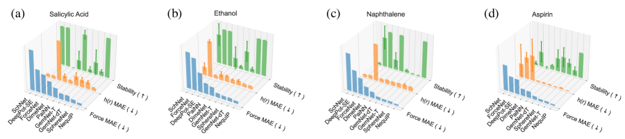
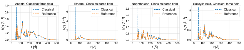
MD17. As shown in Table 3, more recent models that lie on the right side of the table generally achieve a lower force error, but may lack stability. Figure 3 selects and rearranges results from Table 3 to demonstrate the non-aligned trends of force prediction performance vs. simulation performance, which supports key observation 1. SphereNet and GemNet-T/dT can attain a very low force error for all four molecules, but often collapse before the simulation finishes. This observation constitutes key observation 2. We note that although the stable portion of simulated trajectories produced by SphereNet and GemNet-T/dT can recover the $h(r)$ relatively accurately, stability will become a bigger issue when the statistics of interest require long simulations, as demonstrated in other experiments. On the other hand, despite having a relatively high force error, DeepPot-SE performs very well on simulation-based metrics on all molecules except for Aspirin (Figure 3). With the highest molecular weight, Aspirin is indeed the hardest task in MD17 in the sense that all models attain high force prediction errors on it. PaiNN also attains competitive simulation performance, while its force error is not among the best. As a reference, we also include the $h(r)$ error using a popular classical force field: the optimized potentials for liquid simulations (OPLS, Jorgensen & Tirado-Rives 2005) in Table 3. More details on the classical force field results are in Appendix A and Figure 7).

We further observe that good stability alone does not imply accurate recovery of trajectory statistics. Although ForceNet remains stable for Ethanol and Naphthalene, the extracted $h(r)$ deviates a lot from the reference (Table 3), indicating that ForceNet does not learn the underlying PES correctly, possibly due to its lack of energy conservation and rotational equivariance. Overall, NequIP is the best-performing model on MD17. It achieves the best performance in both force prediction and simulation-based metrics for all molecules while requiring the highest computational cost. More detailed results on MD17 including a study on stability’s relation with training epochs and individual $h(r)$ are included in Appendix B.

Table 4: Results on Water-10k. RDF MAE is unit-less. Diffusivity is computed by averaging 5 runs from 5 random initial configurations and its MAE is reported in the unit of [$10^{-9}\ \mathrm{m}^{2}/\mathrm{s}$]. The reference diffusivity coefficient is $2.3\times 10^{-9}\ \mathrm{m}^{2}/\mathrm{s}$.

DeepPot-SE SchNet DimeNet PaiNN SphereNet ForceNet GemNet-T GemNet-dT NequIP Force $(\downarrow)$ $5.8$ $9.5$ $1.4$ $5.1$ $16.1$ $10.9$ $0.7$ $1.3$ $1.5$ Stability $(\uparrow)$ $247_{(147)}$ $232_{(59)}$ $30_{(10)}$ $12_{(13)}$ $500_{(0)}$ $7_{(3)}$ $25_{(7)}$ $7_{(3)}$ $500_{(0)}$ $\mathrm{RDF}_{(O,O)}$ $(\downarrow)$ $0.07_{(0.01)}$ $0.63_{(0.04)}$ $0.27_{(0.15)}$ $0.30_{(0.14)}$ $0.89_{(0.04)}$ $0.79_{(0.03)}$ $0.22_{(0.05)}$ $0.42_{(0.22)}$ $0.06_{(0.02)}$ $\mathrm{RDF}_{(H,H)}$ $(\downarrow)$ $0.06_{(0.02)}$ $0.30_{(0.02)}$ $0.18_{(0.08)}$ $0.21_{(0.09)}$ $0.40_{(0.01)}$ $0.55_{(0.01)}$ $0.16_{(0.03)}$ $0.35_{(0.25)}$ $0.05_{(0.01)}$ $\mathrm{RDF}_{(H,O)}$ $(\downarrow)$ $0.19_{(0.05)}$ $0.57_{(0.04)}$ $0.21_{(0.04)}$ $0.29_{(0.12)}$ $1.14_{(0.03)}$ $1.34_{(0.03)}$ $0.20_{(0.04)}$ $0.42_{(0.27)}$ $0.27_{(0.07)}$ Diffusivity $(\downarrow)$ $0.04$ $1.90$ - - $2.23$ - - - $0.18$ FPS $(\downarrow)$ $91.0$ $78.9$ $17.9$ $71.8$ $3.1$ $67.6$ $11.3$ $33.7$ $3.9$

Figure 4: Comparison of force MAE vs. stability (Left), force MAE vs. RDF MAE (Middle), and force MAE vs. Diffusivity MAE (Right) on the water benchmark. Each model is trained with three dataset sizes. The color of a point indicates the model identity, while the point size indicates the training dataset size (small: 1k, medium: 10k, large: 90k). Metrics infeasible to extract from certain model/dataset size (e.g., Diffusivity for unstable models) are not included.

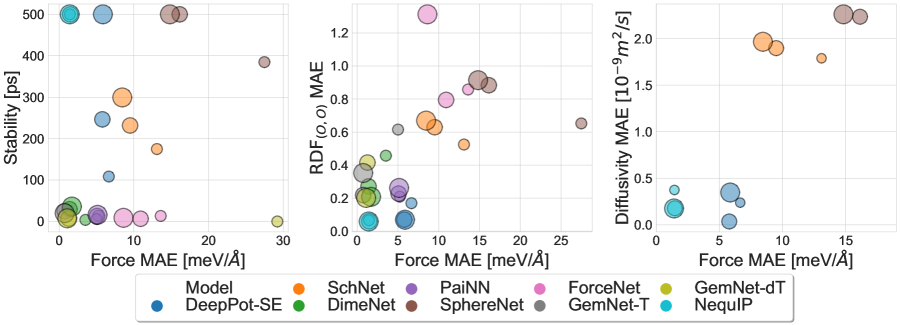
Water. Under a condensed phase system, key observation 1 and 2 are still evident according to Table 4: GemNet-T/dT and DimeNet are the top-3 models in terms of force prediction, but all lack stability. The water diffusivity coefficient requires long (100 ps in our experiments) trajectories to estimate and thus cannot be extracted for unstable models. DeepPot-SE does not achieve the best force prediction performance but demonstrates decent stability and highly accurate recovery of simulation statistics. Interestingly, SphereNet has a high force error but is highly stable. However, the properties are not accurately recovered.

Figure 4 further compares model performance with different training dataset sizes. Key observations 1 and 2 are clearly shown: Models located on the left of each scatter plot have very low force error but may have poor stability or high error in simulation statistics. More specifically, although more training data almost always improve force prediction performance, its effect on simulation performance is not entirely clear. On the one hand, GemNet-T/dT, DimeNet, and ForceNet are not stable even when under the highest training data budget. On the other hand, we observe a clear improvement of DeepPot-SE when more training data is used. NequIP is again the best-performing model, achieving very low force error, excellent stability, and accurate recovery of ensemble statistics, even under the lowest data budget of 1,000 training+validation structures. However, when the training dataset is sufficiently large (90k), DeepPot-SE has equally good results as NequIP while being more than 20 times faster – dataset size also influences the model of choice for a certain dataset. The detailed results for water-1k/90k and the impact of dataset size are included in Appendix B. Furthermore, we also conduct ablation studies on model sizes and training epochs in Appendix B.

Table 5: Results on alanine dipeptide. #Finished is the number of simulations stable for 5 ns. MAE of $F({\phi})$ and $F({\psi})$ are reported in the unit of [$\mathrm{kJ/mol}$].

DeepPot-SE SchNet DimeNet PaiNN SphereNet ForceNet GemNet-T GemNet-dT NequIP Force ($\downarrow$) $272.1$ $217.0$ $239.0$ $266.2$ $256.3$ $284.7$ $233.5$ $219.7$ $215.6$ #Finished ($\uparrow$) 0/6 0/6 0/6 0/6 0/6 0/6 6/6 0/6 5/6 Stability ($\uparrow$) $0_{(0)}$ $0_{(0)}$ $0_{(0)}$ $0_{(0)}$ $804_{(786)}$ $0_{(0)}$ $5000_{(0)}$ $0_{(0)}$ $4169_{(1858)}$ ${F}({\phi})$ ($\downarrow$) - - - - - - $104_{(2)}$ - $104_{(14)}$ ${F}({\psi})$ ($\downarrow$) - - - - - - $110_{(13)}$ - $113_{(36)}$ FPS ($\uparrow$) $54.3$ $42.4$ $12.1$ $42.2$ $9.9$ $99.1$ $15.0$ $36.5$ $8.3$

Alanine dipeptide poses unique challenges in sampling different metastable states separated by high free energy barriers and modeling the implicit solvent. Table 5 shows all models have high force errors due to the random forces introduced by the lack of explicit account of water molecules. Although the force errors are in the same order of magnitude, all models except GemNet-T and NequIP fail to simulate stably. The FES reconstruction task requires stable simulation for the entire 5 ns. GemNet-T and NequIP are the only two models that manage to finish at least one simulation but produce inaccurate statistics. All other models are not stable enough to produce meaningful results. As the key difference between GemNet-T and GemNet-dT is energy conservation, this result suggests a strong stabilization effect of enforcing energy conservation through the prediction of scalar energy. We further analyze the results of this task in Section 7.

Table 6: Results on LiPS. Li-ion Diffusivity coefficient is computed by averaging 5 runs from 5 random initial configurations. The reference Li-ion diffusivity coefficient is $1.35\times 10^{-9}\ \mathrm{m}^{2}/\mathrm{s}$.

DeepPot-SE SchNet DimeNet PaiNN SphereNet ForceNet GemNet-T GemNet-dT NequIP Force ($\downarrow$) $40.5$ $28.8$ $3.2$ $11.7$ $8.3$ $12.8$ $1.3$ $1.4$ $3.7$ Stability ($\uparrow$) $4_{(3)}$ $50_{(0)}$ $48_{(4)}$ $50_{(0)}$ $50_{(0)}$ $26_{(8)}$ $50_{(0)}$ $50_{(0)}$ $50_{(0)}$ RDF ($\downarrow$) $0.27_{(0.15)}$ $0.04_{(0.00)}$ $0.05_{(0.01)}$ $0.04_{(0.01)}$ $0.04_{(0.00)}$ $0.51_{(0.08)}$ $0.04_{(0.00)}$ $0.04_{(0.00)}$ $0.04_{(0.01)}$ Diffusivity ($\downarrow$) - $0.38$ $0.30$ $0.40$ $0.40$ - $0.24$ $0.28$ $0.34$ FPS ($\uparrow$) $66.1$ $35.2$ $14.8$ $75.7$ $18.1$ $72.1$ $16.9$ $43.5$ $8.2$

LiPS. Compared to flexible molecules and liquid water, this solid material system features slower kinetics. From Table 6 we observe that most models are capable of finishing 50-ns simulations stably. In this dataset, the performance on diffusivity estimation and force prediction align well. We observe that both GemNet-T and GemNet-dT show excellent force prediction, stability, and recovery of observables, while GemNet-dT is 2.6 times faster. The better efficiency comes from the direct prediction of atomic forces $\bm{F}$ instead of taking the derivative $\bm{F}=\partial E/\partial\bm{x}$, which also makes GemNet-dT not energy-conserving – a potential issue we further discuss in Section 7.

Implications on model architecture. More recent models utilizing SE(3)/E(3)-equivariant representations and operations such as GemNet-dT and NequIP are more expressive and can capture interatomic interactions more accurately. This is reflected by their very low force error and accurate recovery of ensemble statistics when not bottlenecked by stability. Moreover, excellent accuracy and stability can be simultaneously achieved. The stability may come from parity-equivariance and the use of tensor products (Thomas et al., 2018) in manipulating higher-order geometric features. We believe further investigations into the extrapolation behavior induced by different equivariant geometric representations and operations (Batatia et al., 2022) is a fruitful direction in designing more powerful ML FFs.

7 Failure Modes: Causes and Future Directions

Figure 5: (a, b) For each row, the first three panels show Ramachandran plots of the alanine dipeptide FES reconstructed from 5-ns reference vs. 5-ns NequIP/GemNet-T simulation, all using MetaDynamics. The last two panels show $F(\phi)$ and $F(\psi)$ of alanine dipeptide extracted from reference simulation vs. from NequIP simulation. The two rows result from different initialization, annotated as a yellow star. (c) ($\phi,\psi$) distribution of the alanine dipeptide training dataset. The six initialization points are marked with stars. NequIP fails to remain stable when the simulation starts from the point marked with black color. (d) Model-predicted total energy as a function of simulation time when simulating the LiPS system using the NVE ensemble. (e) On water-10k, stability does not improve when the time step is reduced for GemNet-T.

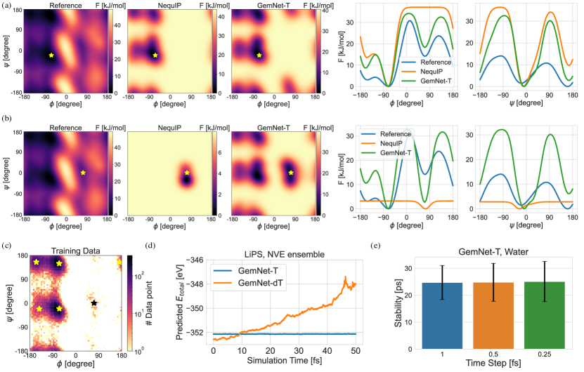
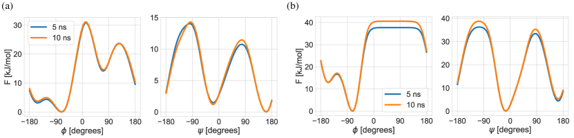
A case study on alanine dipeptide simulation. Figure 5 (a) demonstrates how NequIP and GemNet-T fail to reconstruct the FES: the ML potentials do not manage to sample much of the transition regions and the configuration space with $\phi\in[0,180^{\circ}]$ when initialized from a configuration with $\phi=-65^{\circ}$. Figure 5 (b) shows NequIP fails to simulate stably when initialized from the low-density meta-stable state. The reconstructed FES significantly deviates from the reference in both cases. This failure can be partially explained by Figure 5 (c), the training data distribution produced by the reference potential. The relatively high-energy (low-density) regions and transition regions are exactly those that are not sampled enough by the learned force fields. Even though our MD trajectory is well-equilibrated, the difference in populations of different meta-stable states creates data imbalance, making it more challenging for the model to learn well for higher-energy configurations where density is relatively low. The lack of energy labels for force matching in the implicit solvent setting exacerbated this problem and poses challenges in learning the relative free energy difference between the meta-stable states. This issue implies that generalization across different regions in the conformational space is an important challenge for ML FFs. The rest of the FES results are included in Figure 13.

Energy conservation. Models that directly predict forces may not conserve energy. Figure 5 (d) demonstrates the evolution of model-predicted total energy for selected models on LiPS, in a microcanonical (NVE) ensemble. The energy of an isolated system in the NVE ensemble is, in principle, conserved. We observe that GemNet-T conserves energy, whereas GemNet-dT fails to conserve the predicted total energy. The existence of non-conservative forces breaks the time-reversal symmetry and, therefore, may not be able to reach equilibrium for observable calculation. Energy conservation as an inductive bias can also affect simulation stability. For alanine dipeptide, we observe GemNet-T can achieve stable simulations while GemNet-dT is unstable. On the other hand, GemNet-dT performs well on the LiPS dataset when coupled with a thermostat. Previous works (Kolluru et al., 2022) also found that energy conservation is not required for SOTA performance on OC20. The usability of non-conservative FFs in simulations requires further careful investigations.

Figure 6: Examples of simulation collapse when applying (a) NequIP to alanine dipeptide and (b) GemNet-T to water. The y-axis shows the maximum force observed on any atom in the system at a certain time step. An orange cross indicates visualized time steps. Notable nonphysical regions are circled. The collapse usually happens within a very short period of time after the initial local errors.

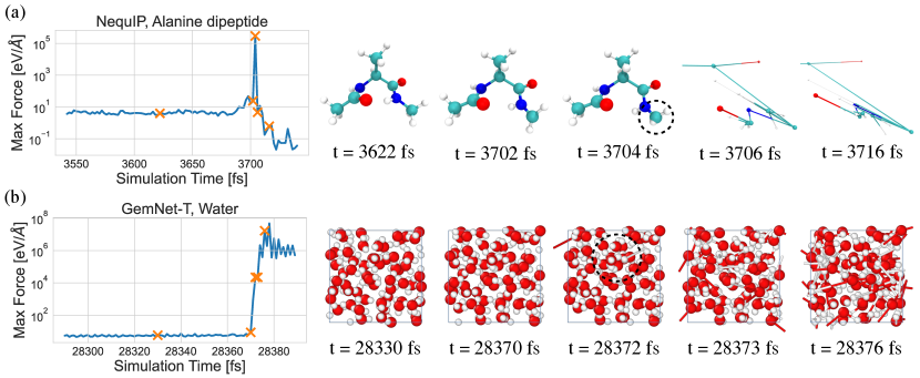
Simulation instability is a major bottleneck for highly accurate models to fail on several simulation tasks. Moreover, in our water experiments, we find a larger amount of training data does not resolve this issue for GemNet-T/dT and DimeNet (Figure 4). We further experiment with smaller simulation time steps for GemNet-T on water (Figure 5 (e)), but stability still does not improve. On the other hand, Stocker et al. (2022) demonstrates that the stability of GemNet improves with larger training sets on QM7-x, which includes high-energy off-equilibrium geometries obtained from normal mode sampling. Normal mode sampling was also used to generate large datasets in earlier ML force fields such as ANI-1 (Smith et al., 2017), and MD simulation results are demonstrated. These results indicate that dataset’s coverage over the conformational space has crucial implications on the behavior of the final model, regardless of the underlying neural network model. We hypothesize that including these distorted geometries may improve the model’s robustness against going into nonphysical configurations. We also observe that the simulation can collapse within a short time window after a long period of stable simulation, as visualized in Figure 6. In both cases, we observe that the nonphysical configurations first emerge at local regions (circled), which cascade to the entire system very quickly as extremely large forces are being predicted and subsequently integrated into the dynamics. At the end of the visualization, the bonds in the alanine dipeptide system are broken. Therefore, the local-descriptor-based NequIP model predicts very small forces. For the water system, the particles are packed in a finite periodic box. The nonphysical configurations exhibit incorrect coordination structures and extremely large forces. To prevent ML FFs from sampling nonphysical regions, which is a common precursor to failed simulation (Figure 6), one can deliberately include distorted and off-equilibrium geometries in the training data to improve model robustness(Stocker et al., 2022). Alternatively, one can resort to active learning (Wang et al., 2020b; Vandermause et al., 2020; Schwalbe-Koda et al., 2021) to acquire new data points based on model uncertainty. Past works also found adding noise to data paired with a denoising objective during training helpful in improving out-of-distribution test performance on OC20 (Godwin et al., 2021), and in stabilizing learned simulations (Sanchez-Gonzalez et al., 2020). Another relevant line of work in coarse-grained MD simulation has studied regularization with an empirical “prior energy” (Wang et al., 2019b) and post-prediction refinement (Fu et al., 2022) to battle simulation instability.

8 Conclusion and Outlook

We have introduced a diverse suite of MD simulation tasks and conducted a thorough comparison of SOTA ML FFs to reveal novel insights into ML for MD simulation. As shown in our experiments, benchmarking only force error is not sufficient, and simulation-based metrics should be used to reflect the practical utility of a model. We demonstrate case studies on the failure of existing training schemes/models to better understand their limitations. The performance of a model can be highly case-dependent. For more challenging MD systems, more expressive atomistic representations may be required. For example, recent work has explored non-local descriptors (Kabylda et al., 2022) aiming at capturing long-range interactions in large molecules. Strictly local equivariant representations (Musaelian et al., 2022) are studied for large systems where computational scalability is critical. New datasets (Eastman et al., 2022) and benchmarks have been playing an important role in inspiring future work. Learning coarse-grained MD (Wang et al., 2019b; Wang & Gómez-Bombarelli, 2019; Fu et al., 2022) is another avenue to accelerate MD at larger length/time scales.

The possibility of ML in advancing MD simulation is not limited to ML force fields. Enhanced sampling methods enable fast sampling of rare events and have been augmented with ML techniques (Schneider et al., 2017; Sultan et al., 2018; Holdijk et al., 2022). Differentiable simulations (Schoenholz & Cubuk, 2020; Wang et al., 2020a; Doerr et al., 2021; Ingraham et al., 2018; Greener & Jones, 2021) offer a principled way of learning the force field by directly training the simulation process to reproduce experimental observables (Wang et al., 2020a; 2022; Thaler & Zavadlav, 2021). We hope our datasets and benchmarks will encourage future developments in all related aspects to push the frontier in ML for MD simulations.

Author Contributions

X.F. led the project. X.F., Z.W., W.W., and T.X. designed the benchmark and evaluation protocols; Z.W. performed MD simulations to generate datasets; X.F. implemented the models and performed the experiments; X.F.,Z.W.,W.W., T.X., and T.J. analyzed the results; X.F., Z.W., W.W., T.X., S.K., R.G.B., and T.J. wrote the manuscript.

Acknowledgments

We thank Adrian Roitberg and the Roitberg Research Group for their valuable suggestions on rectifying our alanine dipeptide evaluation protocol. We thank Adeesh Kolluru, Simon Batzner, and Alby Musaelian for helping with reproducing previous results. X.F. is supported by the MIT-GIST collaboration. W.W. is supported by Toyota Research Institute. Z.W. is supported by the Center for Hierarchical Materials Design at Northwestern University and Army Research Office. The authors also acknowledge the MIT SuperCloud and the Lincoln Laboratory Supercomputing Center for providing HPC resources. We also acknowledge PyTorch and PyTorch Geometric.

Appendix A Dataset details

Figure 7: Comparison between a classical force field and the reference simulation on the $h(r)$ of MD17 molecules.

The MD17 dataset (Chmiela et al., 2017) and the LiPS dataset (Batzner et al., 2022) are adapted from previous works and are publicly available. The MD17 dataset is generated from path-integral molecular dynamics simulations that incorporate quantum mechanics into the classic molecular dynamics simulations using Feynman path integrals. The LiPS datasets are generated by ab-initio molecular dynamics simulations with a generalized gradient PBE functional and projector augmented wave pseudopotentials. We refer interested readers to the respective papers for more details on the data generation process. The water dataset and alanine dipeptide dataset are generated by ourselves, and the generation process is explained in the next paragraphs.

To demonstrate how ML force fields can improve simulation accuracy over classical force fields, we also simulated the four MD17 molecules with a popular classical force field: the optimized potentials for liquid simulations (OPLS, Jorgensen & Tirado-Rives 2005) with OpenMM (Eastman et al., 2017). In OPLS, interatomic interactions are described by a combination of simple functional forms, such as harmonic and Lennard-Jones potentials, for bond stretch, bond angle, torsional angle, and pair-wise non-bonded interactions. We sample the molecule conformations in vacuum under an NVT ensemble with a timestep of 1 femtosecond and temperature of 500 K, controlled with a Langevin thermostat. The resulting $h(r)$ from the classical force field is compared to the reference in Figure 7. The errors it attains are reported in Table 3, which are much higher than most ML force fields, whose $h(r)$ curves are shown in Figure 14.

Water. Our water dataset is generated from molecular dynamics simulations of a simple classical water model, namely, the flexible version of the Extended Simple Point Charge water model (SPC/E-fw) (Wu et al., 2006) at temperature $T=300$ K and pressure $P=1$ atm. For this model, the interaction parameters (e.g., O-H bond stretch and H-O-H bond angles), are parameterized to match extensive experimental properties such as the self-diffusion and dielectric constants at bulk phase. This classical model has been well-studied in previous work (Wu et al., 2006; Yue et al., 2021) and has shown reasonable predictions of the physical properties of liquid water. It provides a computationally inexpensive way to generate a large amount of training data. The experience and knowledge gained from the benchmark based on the simple model can be readily extended to systems with higher accuracy, such as the ab-initio models.

Alanine dipeptide. Our dataset is generated from the MD simulation of an alanine dipeptide molecule solvated in explicit water (1164 water molecules) performed in GROMACS (Abraham et al., 2015) using the AMBER-03 (Ponder & Case, 2003b) force-field. In the AMBER-03 force field, the potential energy parameters such as van der Waals and electrostatics are mostly derived from quantum mechanical methods with minor optimization on the bonded parameters to reproduce the experimental vibrational frequencies and structures (Cornell et al., 1996; Ponder & Case, 2003a). The NPT ensemble is applied in simulations, with hydrogen bond length constraints using LINear Constraint Solver (LINCS) and a time step of 2 fs. The temperature and pressure of the system are controlled at $T=300$ K and $P=1$ bar using a stochastic velocity rescaling thermostat with damping frequency $t_{v}=0.1$ ps and Parrinello-Rahman barostat with coupling frequency $t_{p}=2.0$ ps, respectively. The Particle Mesh Ewald approach is used to compute long-range electrostatics with periodic boundary conditions applied to the x, y, and z directions. The conformational modes can be characterized by six free energy local minima, which have been used in previous work (Lederer et al., 2022). We initialize six simulations for each model from each of the six free energy local minima.

Figure 8: $F(\phi)$ and $F(\psi)$ have converged for the reference force field (a) and NequIP (b) at time 5 ns under Metadynamics.

Implicit solvation. The explicit solvent of 1164 water molecules is not the subject of study but adds a significant computational burden. In this task, we attempt to learn an implicit solvent model (ISM) of the alanine dipeptide, in which the explicit solvent environment is incorporated in the learned FF. The ISM is commonly used in drug design (Wang et al., 2019a) because it can speed up the computation by dramatically decreasing the number of particles required for simulation. In general, the mean-field estimation in ISM ignores the effect of solvent, thermal fluctuations, and solvent friction (Feig, 2007). Thus, molecular kinetics is not directly comparable to the explicit solvation simulation. However, the equilibrium configurations can be explicitly compared, as conducted in Chen et al. (2021).

Metadynamics simulation. Simulating energy barrier jump usually requires a long sampling of the trajectory in MD simulations. The conformational change of alanine dipeptide in water involves such a process, making it difficult to extract the complete free energy surface, i.e., the Ramachandran plot, in normal MD. In order to examine the learned ML FFs within a reasonable time limit, metadynamics (Laio & Parrinello, 2002) is employed to explore the learned FES of the solvated alanine dipeptide. Metadynamics is a widely used technique in atomistic simulations to accelerate the sampling of rare events and estimate the FES of a certain set of degrees of freedom. It is based on iteratively “filling” the potential energy using a sum of Gaussians deposited on a set of suitable collective variables (CVs) along the trajectory. At evaluation time, we perform metadynamics with dihedral angles $\phi$ and $\psi$ as CVs, starting from the configurations located at one of the six energy minimums in the free energy surface indicated in Figure 5 (c). The Gaussians with height $h=1.2$ and sigma $\sigma=0.35$ are deposited every 1 ps centered on $\psi$ and $\phi$. As shown in Figure 8, the estimated FES of both $\phi$ and $\psi$ do not significantly change after 5 ns. In addition, the height of the bias gaussian potential smoothly converges to $\sim 0$ in the time limit of $5$ ns. Therefore, a simulation time of 5 ns is sufficient for the convergence of the metadynamics. This metadynamics simulation of alanine dipeptide with AMBER force fields is carried out using GROMACS (Abraham et al., 2015) integrated with the PLUMED library (Tribello et al., 2014; Colón-Ramos et al., 2019) of version 2.8.

Figure 9: (a) The distribution of bond length deviation for the Aspirin reference dataset. Black dashed line is our chosen stability threshold. (b) An example simulated trajectory of Aspirin using SchNet that becomes unstable. Y-axis is log-scaled. (c) The distribution of RDF deviation for the water reference dataset. Black dashed line is our chosen stability threshold. (d) An example simulated trajectory of Water-10k using GemNet-T that becomes unstable.

Appendix B Experimental details

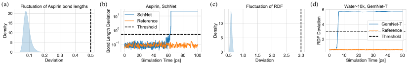
Selection of stability threshold. Our stability thresholds are chosen to be relaxed, so a simulation is only flagged as “unstable” when the system has already went into highly non-realistic configurations. In Figure 9 (a) and (c), we show the natural fluctuation existing in the reference data of $\mathrm{RDF}$ for water and bond lengths for Aspirin, demonstrating that realistic simulations would never exceed the stability thresholds. In our experiments, unstable simulations cannot recover from catastrophic failure to become stable again. Example trajectories using SchNet on Aspirin and GemNet-T on water are shown in Figure 9 (b) and (d).

Figure 10: 3D symmetries that ML force fields should respect include translations, rotations, and reflections.

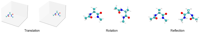
Symmetry principles. the learned force fields should respect the symmetry principles: energy is permutational invariant and E(3)-invariant, and forces are permutational invariant and E(3)-equivariant. E(3) comprises translations, rotations, and reflections in 3D (Figure 10). A function $f$ is $G$-equivariant if $f\circ T=L\circ f$ for some operator $L$, where $T$ is an operator for transformation in $G$. $f$ is invariant if $f\circ T=f$. For example, the energy prediction of a $E(3)$-invariant model will be invariant with represet to 3D rotation, translation, and reflection of the input structure. Our benchmark includes various models with different levels of symmetry principles (Table 2) and thus have different expressive power.

Experimental procedures. Baseline models are trained on the datasets described in Section 4 according to the experimental settings described in Appendix B. At evaluation time, we simulate MD trajectories using the learned models, with thermostats and simulation length described in Section 4. The simulated trajectories are recorded as time series of atom positions, along with other information including atom types, temperature, total energy, potential energy, and kinetic energy. All observables described in this section can be computed from recorded trajectories. We use the stability criterion described above to find the time step when the systems become “unstable”, and only use the trajectory before that time step for the computation of observables. Among the observables, the distribution of interatomic distances and RDF are computed for each frame and averaged over the entire trajectory. Diffusivity coefficients are computed by averaging over the diffusivity coefficient computed from all applicable time windows where the time window length is predefined to be long enough. For example, for a trajectory of $T$ steps and a time window of $K$ steps, we average over the diffusivity computed from the time windows: $[1,K],[2,K+1],\dots,[T-K+1,T]$. We use 100 ps as the time window size for water and 35 ps as the time window size for LiPS. We also remove the first 5 ps of the simulated trajectories of LiPS for equilibrium. As we do multiple simulations per model and dataset, we compute the metrics for each trajectory and report the mean and standard deviation. When reporting the efficiency of different models, all frames per second (FPS) metrics are measured with an NVIDIA Tesla V100-PCIe GPU. We present FPS as a reference for models’ computational efficiency but also note that code speed can be affected by many factors and likely has room for improvement. Further details on observable computation can be found in our code submission: observable.ipynb. The Open Catalyst Project codebase and the official codebases of DeepPot-SE, SphereNet, and NequIP are all publicly available. We build our MD simulation framework based on the Atomic Simulation Environment (ASE) library (Larsen et al., 2017).

Table 7: Default training-related hyperparameters for each dataset. ^*We adopt the original batch size from respective papers when available for MD17. DeepPot-SE: 4; SchNet: 100; DimeNet: 32; GemNet-T/dT: 1; NequIP: 5. We use a batch size of 8 for ForceNet.

Dataset Training dataset size Batch size Max epoch LR patience Longest simulation time MD17 9,500 1-100^* 2,000 5 epochs 20 hours Water-1k 950 1 10,000 50 epochs 28 hours Water-10k 9,500 1 2,000 5 epochs 28 hours Water-90k 85,500 1 400 3 epochs 28 hours Alanine dipeptide 38,000 5 2,000 5 epochs 75 hours LiPS 19,000 1 2,000 5 epochs 7 hours

Table 8: Results on Water-1k. Force MAE is reported in the unit of [meV/Å]; Stability is reported in the unit of [ps]; Diffusivity MAE is reported in the unit of [$10^{-9}\ \mathrm{m}^{2}/\mathrm{s}$]; RDF MAE and FPS are unitless.

DeepPot-SE SchNet DimeNet PaiNN SphereNet ForceNet GemNet-T GemNet-dT NequIP Force $6.7$ $13.1$ $3.5$ $5.2$ $27.5$ $13.6$ $5.0$ $29.2$ $1.4$ Stability $108_{(117)}$ $175_{(56)}$ $4_{(4)}$ $14_{(9)}$ $385_{(160)}$ $13_{(7)}$ $6_{(7)}$ $0_{(0)}$ $500_{(0)}$ $\mathrm{RDF}_{(O,O)}$ $0.17_{(0.10)}$ $0.52_{(0.05)}$ $0.46_{(0.22)}$ $0.21_{(0.05)}$ $0.65_{(0.02)}$ $0.86_{(0.09)}$ $0.62_{(0.48)}$ - $0.07_{(0.02)}$ $\mathrm{RDF}_{(H,H)}$ $0.13_{(0.09)}$ $0.24_{(0.02)}$ $0.33_{(0.15)}$ $0.15_{(0.04)}$ $0.29_{(0.01)}$ $0.56_{(0.04)}$ $0.35_{(0.21)}$ - $0.07_{(0.02)}$ $\mathrm{RDF}_{(H,O)}$ $0.28_{(0.15)}$ $0.54_{(0.01)}$ $0.43_{(0.17)}$ $0.16_{(0.04)}$ $0.81_{(0.03)}$ $1.44_{(0.09)}$ $0.71_{(0.65)}$ - $0.26_{(0.07)}$ Diffusivity $0.24$ $1.79$ - - $2.05$ - - - $0.37$ FPS $61.8$ $99.2$ $16.4$ $54.5$ $3.0$ $68.1$ $15.4$ $34.5$ $3.9$

Table 9: Results on Water-90k. Force MAE is reported in the unit of [meV/Å]; Stability is reported in the unit of [ps]; Diffusivity MAE is reported in the unit of [$10^{-9}\ \mathrm{m}^{2}/\mathrm{s}$]; RDF MAE and FPS are unitless.

DeepPot-SE SchNet DimeNet PaiNN SphereNet ForceNet GemNet-T GemNet-dT NequIP Force $5.9$ $8.4$ $1.7$ $5.1$ $14.8$ $8.6$ $0.7$ $1.1$ $1.4$ Stability $500_{(0)}$ $299_{(70)}$ $36_{(9)}$ $16_{(7)}$ $500_{(0)}$ $9_{(12)}$ $20_{(9)}$ $8_{(10)}$ $500_{(0)}$ $\mathrm{RDF}_{(O,O)}$ $0.07_{(0.02)}$ $0.67_{(0.03)}$ $0.21_{(0.03)}$ $0.26_{(0.17)}$ $0.91_{(0.04)}$ $1.31_{(0.49)}$ $0.35_{(0.23)}$ $0.20_{(0.01)}$ $0.06_{(0.01)}$ $\mathrm{RDF}_{(H,H)}$ $0.05_{(0.01)}$ $0.31_{(0.02)}$ $0.14_{(0.01)}$ $0.20_{(0.12)}$ $0.42_{(0.03)}$ $0.82_{(0.26)}$ $0.25_{(0.19)}$ $0.16_{(0.01)}$ $0.04_{(0.01)}$ $\mathrm{RDF}_{(H,O)}$ $0.29_{(0.08)}$ $0.67_{(0.04)}$ $0.18_{(0.02)}$ $0.21_{(0.06)}$ $1.24_{(0.08)}$ $2.05_{(0.60)}$ $0.24_{(0.06)}$ $0.26_{(0.02)}$ $0.25_{(0.06)}$ Diffusivity $0.35$ $1.97$ - - $2.26$ - - - $0.18$ FPS $62.1$ $103.0$ $16.3$ $71.9$ $3.1$ $43.8$ $15.3$ $32.7$ $3.0$

Table 10: Water-1k results on NequIP with various model sizes and radius cutoffs.

Force Stability $\mathrm{RDF}_{(O,O)}$ $\mathrm{RDF}_{(H,H)}$ $\mathrm{RDF}_{(H,O)}$ Diffusivity FPS Width=64, r=4 $3.5$ $500_{(0)}$ $0.07_{(0.02)}$ $0.05_{(0.01)}$ $0.27_{(0.06)}$ $0.38$ $8.2$ Width=32, r=6 $1.5$ $500_{(0)}$ $0.06_{(0.01)}$ $0.05_{(0.01)}$ $0.26_{(0.06)}$ $0.25$ $5.2$ Width=64, r=5 $1.6$ $500_{(0)}$ $0.07_{(0.02)}$ $0.05_{(0.01)}$ $0.27_{(0.06)}$ $0.31$ $4.9$ Width=64, r=6 $1.4$ $500_{(0)}$ $0.07_{(0.02)}$ $0.07_{(0.02)}$ $0.26_{(0.07)}$ $0.37$ $3.9$ Width=128, r=6 $1.5$ $500_{(0)}$ $0.07_{(0.02)}$ $0.05_{(0.01)}$ $0.29_{(0.07)}$ $0.37$ $2.5$

Table 11: Results on the large water system with 512 molecules, with models trained on the water-10k dataset (64-molecule water system). ^*SphereNet on Water-large requires more memory than Tesla V100 supports. We run its simulations on faster NVIDIA A100 cards so the FPS is not entirely comparable to other models.

DeepPot-SE SchNet DimeNet PaiNN SphereNet^* ForceNet GemNet-T GemNet-dT NequIP Force $10.6$ $12.1$ $5.1$ $9.7$ $18.4$ $13.2$ $5.6$ $4.2$ $7.7$ Stability $19_{(22)}$ $118_{(58)}$ $38_{(13)}$ $16_{(12)}$ $150_{(0)}$ $8_{(0)}$ $45_{(25)}$ $50_{(9)}$ $150_{(0)}$ $\mathrm{RDF}_{(O,O)}$ $0.23_{(0.06)}$ $0.62_{(0.01)}$ $0.17_{(0.03)}$ $0.31_{(0.06)}$ $0.93_{(0.02)}$ $0.74_{(0.02)}$ $0.22_{(0.16)}$ $0.16_{(0.02)}$ $0.10_{(0.01)}$ $\mathrm{RDF}_{(H,H)}$ $0.24_{(0.06)}$ $0.30_{(0.04)}$ $0.12_{(0.03)}$ $0.21_{(0.05)}$ $0.42_{(0.01)}$ $0.51_{(0.02)}$ $0.15_{(0.11)}$ $0.11_{(0.01)}$ $0.07_{(0.00)}$ $\mathrm{RDF}_{(H,O)}$ $0.67_{(0.27)}$ $0.55_{(0.01)}$ $0.17_{(0.02)}$ $0.29_{(0.05)}$ $0.97_{(0.03)}$ $1.38_{(0.05)}$ $0.23_{(0.12)}$ $0.16_{(0.02)}$ $0.12_{(0.02)}$ Diffusivity - $2.54$ - - $2.98$ - - - $0.89$ FPS $80.7$ $23.1$ $3.5$ $17.4$ $0.8$ $11.9$ $2.2$ $5.3$ $0.7$

Hyperparameters. We adopt the original model hyperparameters in the respective papers and find they can produce good force prediction results that match the trend and numbers for MD17 reported in previous work. As we introduce new datasets, we set training hyperparameters such as the batch size and summarize them in Table 7. For water and LiPS, we use a batch size of 1 like in previous work (Batzner et al., 2022) as each structure already contains a reasonable number of atoms and interactions. Following previous work, we use an initial learning rate of 0.001 for all experiments except for NequIP, which uses 0.005 as the initial learning rate in the original paper. For models that minimize a mixture of force loss and energy loss, we set the force loss coefficient $\lambda_{F}$ to be $1000$ and the energy loss coefficient $\lambda_{E}$ to be $1$, if not specified in the original paper. A higher force loss coefficient is common in previous work (Zhang et al., 2018a; Batzner et al., 2022) as simulations do not directly rely on the energy.

Notably, NequIP proposed several sets of hyperparameters for different datasets, including MD17, a water+ice dataset from Zhang et al. 2018a, LiPS, etc. We follow the MD17 hyperparameters of NequIP for our MD17 and alanine dipeptide datasets; the water+ice hyperparameters of NequIP for our water dataset; and the LiPS hyperparameters of NequIP for the same LiPS dataset. For DeepPot-SE, we adopted hyperparameters introduced in Zhang et al. 2018a. The only architectural adjustment we made is because we observed training instability for ForceNet on water using the original hyperparameters. We resolve this issue by reducing the network width from 512 to 128 for ForceNet in our water experiments.

To facilitate benchmarking with a reasonable computational budget, we stop the training of a model if either of the following conditions is met: (1) a maximum training time of 7 days is reached on an NVIDIA Tesla V100-PCIe GPU; (2) a maximum number of epochs specified in Table 7 is reached; (3) The learning rate drops below $10^{-6}$ with a ReduceLROnPlateau scheduler with factor 0.8 and learning rate (LR) patience specified in Table 7. We also report the longest time for an ML model to finish our benchmark simulation in Table 7. All numbers are results of NequIP. The high computational cost for evaluating MD simulations has been a major consideration in designing our benchmark datasets and metrics. Training of DeepPot-SE is efficient and we follow the training setup specified in Zhang et al. 2018a.

Complete water results. We present results on water-1k in Table 8 and results on water-90k in Table 9. Results on water-10k is presented in Table 4 in the main text. All models generally achieve lower force error when trained with more data, but stability and estimation of ensemble statistics don’t necessarily improve. In particular, DeepPot-SE shows clear improvement with more training data and becomes as good as NequIP on water-90k. SchNet demonstrates significant improvement in stability, but the estimation of ensemble statistics does not improve. This may be due to the limited accuracy of SchNet coming from the limited expressiveness of the invariant atomic representation.

Figure 11: The force error and stability of SchNet for simulating Salicylic acid, as training progress.

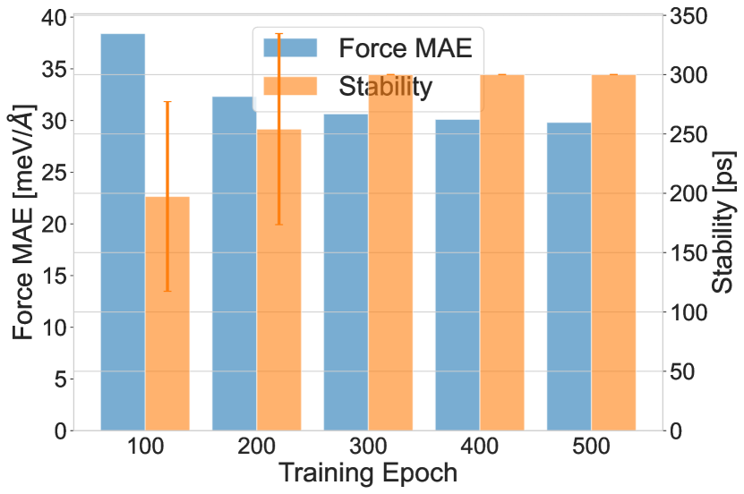
Large water system of 512 molecules. To study model performance in generalizing to a larger system and model scalability, we evaluate models trained on the water-10k dataset on a dataset with 512 water molecules simulated for 1 ns, using the same reference force field. Given the high cost of simulating a large system, we simulate 5 trajectories of 150 ps long for each model. The results are shown in Table 11. We observe that all models suffer slightly higher force errors compared to the evaluation of the 64-molecule water system. In terms of stability, NequIP and SphereNet always remain stable for the entire 150 ps. However, SphereNet does not produce correct ensemble properties. SchNet is the third stable model, while all other models are not stable enough for diffusivity computation. DimeNet, GemNet-T, and GemNet-dT are not stable throughout the entire simulation but can produce decent RDF results. Noticeably, the stability of DeepPot-SE drops significantly. We hypothesize that the lack of message passing limits its capability in capturing long-range interactions and thus limits the performance in a larger system.

Influence of model size. Table 10 shows an ablation study over the model size and radius cutoff of NequIP over water-1k. We observe that all models are highly stable and attain equally good performance in simulation-based metrics. Although a small radius cutoff of $4$ leads to worse performance in force prediction, it is more computationally efficient and preserves the trajectory statistics. These results show that there exists a trade-off between accuracy and efficiency when choosing the hyperparameters of an ML force field, and force error may not be the preferred criterion for model selection.

Stability’s relation with dataset size. We extract the force and stability results for each model from Figure 4 to make Figure 12 to better illustrate the relation between stability and dataset size for each model. We observe that while more data almost always reduce force error, stability does not necessarily improve. In particular, NequIP is highly stable across all dataset sizes. DeepPot-SE and SchNet have significant improvements in stability with more data. While for DimeNet ForceNet, and GemNet, more training data does not bring significant stability improvement. Section 7 contains detailed discussions on the causes of instability and potential solutions to improve stability.

Stability’s relation with training epochs. We study the evolution of simulation stability in the training process of an ML force field. We take the SchNet model on the MD17 molecule salicylic acid and save the checkpoint at 100, 200, 300, 400, and 500 epochs. We conduct 5 simulations of 300 ps using each checkpoint. Figure 11 shows the force error and stability of the model at different stages of training. We observe that the force error decreases as training progresses, and the stability improves to be stable across the entire 300 ps simulation and training epoch 300. This result reveals that thorough training is important to both the accuracy and stability of ML force fields.

Table 12: Results on Water-10k-time-split. Force MAE is reported in the unit of [meV/Å]; Stability is reported in the unit of [ps]; Diffusivity MAE is reported in the unit of [$10^{-9}\ \mathrm{m}^{2}/\mathrm{s}$]; RDF MAE and FPS are unitless.

DeepPot-SE SchNet DimeNet PaiNN SphereNet ForceNet GemNet-T GemNet-dT NequIP Force $5.8$ $10.1$ $1.2$ $6.6$ $18.4$ $12.3$ $0.7$ $1.3$ $1.7$ Stability $171_{(152)}$ $353_{(87)}$ $10_{(9)}$ $14_{(9)}$ $500_{(0)}$ $2_{(0)}$ $21_{(11)}$ $15_{(13)}$ $500_{(0)}$ $\mathrm{RDF}_{(O,O)}$ $0.08_{(0.03)}$ $0.75_{(0.06)}$ $0.28_{(0.14)}$ $0.33_{(0.13)}$ $0.99_{(0.05)}$ $0.75_{(0.00)}$ $0.19_{(0.06)}$ $0.35_{(0.17)}$ $0.05_{(0.01)}$ $\mathrm{RDF}_{(H,H)}$ $0.06_{(0.02)}$ $0.34_{(0.03)}$ $0.16_{(0.04)}$ $0.18_{(0.04)}$ $0.43_{(0.03)}$ $0.56_{(0.01)}$ $0.12_{(0.02)}$ $0.22_{(0.12)}$ $0.04_{(0.00)}$ $\mathrm{RDF}_{(H,O)}$ $0.18_{(0.07)}$ $0.73_{(0.01)}$ $0.18_{(0.03)}$ $0.21_{(0.05)}$ $1.22_{(0.03)}$ $1.28_{(0.01)}$ $0.16_{(0.01)}$ $0.16_{(0.04)}$ $0.21_{(0.04)}$ Diffusivity $0.15$ $2.04$ - - $2.25$ - - - $0.25$ FPS $62.0$ $100.5$ $17.1$ $57.3$ $2.9$ $62.2$ $15.1$ $32.5$ $3.5$

Water-10k with a time split. We investigate a time split of the water dataset by using the first 10,000 structures for training and the last 10,000 structures for testing. The results are reported in Table 12. We find most models perform slightly worse compared to the random split results in Table 4, while the trend of performance ranking stays the same.

Distribution of interatomic distances for MD17. Figure 14 shows the $h(r)$ curves for all models and molecules benchmarked. We randomly selected one simulation out of the five simulations we conducted for each model and molecule. We observe that due to lack of stability, DeepPot-SE produces noisy $h(r)$ on Aspirin. ForceNet does not manage to learn the correct interatomic interactions and produces incorrect $h(r)$ curves. Most models are able to produce $h(r)$ that match well with the reference, with SchNet being less accurate on Aspirin and Ethanol.

Figure 12: The force error and stability of all models on the water dataset, with varying training dataset size: 1k, 10k, and 90k.

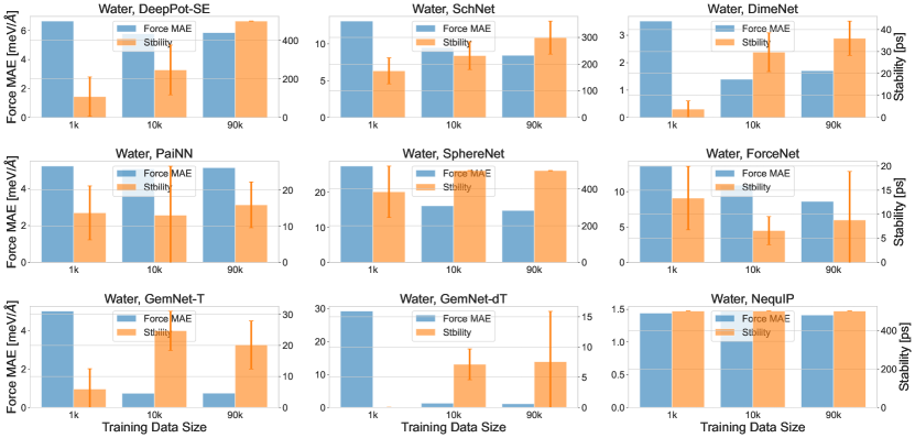
RDFs for water. Selected RDF curves for water-1k/10k/90k are in Figure 15, Figure 16, and Figure 17. Most noisy curves are due to insufficient sampling time, which results in a small number of frames to be averaged in obtaining the RDF curves. We observe that SchNet and ForceNet produce inaccurate curves that are not very noisy, showing that their failure is not entirely due to a lack of stability but because of inaccurate modeling of interactions caused by limited expressiveness and lower sample efficiency. Further, we note that the reference curves have zero values below a certain threshold, as any pair of atoms cannot get too close to each other. However, DimeNet and GemNet-T exhibit abnormally high values for very small distances, indicating the simulations have gone into nonphysical configurations and collapsed.

RDFs for LiPS. As shown in Figure 18, DeepPot-SE does not manage to stay stable on LiPS. ForceNet learns inaccurate interactions and produces inaccurate RDFs. All other models can produce highly accurate RDF and can reproduce Li-ion diffusivity relatively accurately, as demonstrated in Table 6.

Figure 13: Alanine dipeptide FES results from different initialization.

Figure 14: h(r) of md17.

Figure 15: RDFs of Water-1k. GemNet-dT does not remain stable for more than 1 ps and is therefore not feasible for RDF computation.

Figure 16: RDFs of Water-10k.

Figure 17: RDFs of Water-90k.

Figure 18: RDFs of LiPS.

References

- Abraham et al. (2015) Mark James Abraham, Teemu Murtola, Roland Schulz, Szilárd Páll, Jeremy C. Smith, Berk Hess, and Erik Lindahl. GROMACS: High performance molecular simulations through multi-level parallelism from laptops to supercomputers. SoftwareX, 1-2:19–25, September 2015. ISSN 23527110. doi: 10.1016/j.softx.2015.06.001. URL https://linkinghub.elsevier.com/retrieve/pii/S2352711015000059.
- Alder & Wainwright (1959) Berni J Alder and Thomas Everett Wainwright. Studies in molecular dynamics. i. general method. The Journal of Chemical Physics, 31(2):459–466, 1959.
- Artrith et al. (2017) Nongnuch Artrith, Alexander Urban, and Gerbrand Ceder. Efficient and accurate machine-learning interpolation of atomic energies in compositions with many species. Physical Review B, 96(1):014112, 2017.
- Batatia et al. (2022) Ilyes Batatia, Simon Batzner, Dávid Péter Kovács, Albert Musaelian, Gregor NC Simm, Ralf Drautz, Christoph Ortner, Boris Kozinsky, and Gábor Csányi. The design space of e (3)-equivariant atom-centered interatomic potentials. arXiv preprint arXiv:2205.06643, 2022.
- Batzner et al. (2022) Simon Batzner, Albert Musaelian, Lixin Sun, Mario Geiger, Jonathan P Mailoa, Mordechai Kornbluth, Nicola Molinari, Tess E Smidt, and Boris Kozinsky. E (3)-equivariant graph neural networks for data-efficient and accurate interatomic potentials. Nature communications, 13(1):1–11, 2022.
- Behler & Parrinello (2007) Jörg Behler and Michele Parrinello. Generalized neural-network representation of high-dimensional potential-energy surfaces. Physical review letters, 98(14):146401, 2007.
- Chanussot et al. (2021) Lowik Chanussot, Abhishek Das, Siddharth Goyal, Thibaut Lavril, Muhammed Shuaibi, Morgane Riviere, Kevin Tran, Javier Heras-Domingo, Caleb Ho, Weihua Hu, et al. Open catalyst 2020 (oc20) dataset and community challenges. ACS Catalysis, 11(10):6059–6072, 2021.
- Chen & Ong (2022) Chi Chen and Shyue Ping Ong. A universal graph deep learning interatomic potential for the periodic table. Nature Computational Science, 2(11):718–728, 2022.
- Chen et al. (2021) Yaoyi Chen, Andreas Krämer, Nicholas E Charron, Brooke E Husic, Cecilia Clementi, and Frank Noé. Machine learning implicit solvation for molecular dynamics. The Journal of Chemical Physics, 155(8):084101, 2021.
- Chmiela et al. (2017) Stefan Chmiela, Alexandre Tkatchenko, Huziel E Sauceda, Igor Poltavsky, Kristof T Schütt, and Klaus-Robert Müller. Machine learning of accurate energy-conserving molecular force fields. Science advances, 3(5):e1603015, 2017.
- Colón-Ramos et al. (2019) Daniel A. Colón-Ramos, Patrick La Riviere, Hari Shroff, and Rudolf Oldenbourg. Transforming the development and dissemination of cutting-edge microscopy and computation. Nat Methods, 16(8):667–669, August 2019. ISSN 1548-7091, 1548-7105. doi: 10.1038/s41592-019-0475-y. URL http://www.nature.com/articles/s41592-019-0475-y.
- Cornell et al. (1996) Wendy D Cornell, Piotr Cieplak, Christopher I Bayly, Ian R Gould, Kenneth M Merz, David M Ferguson, David C Spellmeyer, Thomas Fox, James W Caldwell, and Peter A Kollman. A second generation force field for the simulation of proteins, nucleic acids, and organic molecules j. am. chem. soc. 1995, 117, 5179- 5197. Journal of the American Chemical Society, 118(9):2309–2309, 1996.
- Doerr et al. (2021) Stefan Doerr, Maciej Majewski, Adrià Pérez, Andreas Kramer, Cecilia Clementi, Frank Noe, Toni Giorgino, and Gianni De Fabritiis. Torchmd: A deep learning framework for molecular simulations. Journal of chemical theory and computation, 17(4):2355–2363, 2021.
- Eastman et al. (2017) Peter Eastman, Jason Swails, John D Chodera, Robert T McGibbon, Yutong Zhao, Kyle A Beauchamp, Lee-Ping Wang, Andrew C Simmonett, Matthew P Harrigan, Chaya D Stern, et al. Openmm 7: Rapid development of high performance algorithms for molecular dynamics. PLoS computational biology, 13(7):e1005659, 2017.
- Eastman et al. (2022) Peter Eastman, Pavan Kumar Behara, David L. Dotson, Raimondas Galvelis, John E. Herr, Josh T. Horton, Yuezhi Mao, John D. Chodera, Benjamin P. Pritchard, Yuanqing Wang, Gianni De Fabritiis, and Thomas E. Markland. Spice, a dataset of drug-like molecules and peptides for training machine learning potentials, 2022.
- Faber et al. (2017) Felix A Faber, Luke Hutchison, Bing Huang, Justin Gilmer, Samuel S Schoenholz, George E Dahl, Oriol Vinyals, Steven Kearnes, Patrick F Riley, and O Anatole Von Lilienfeld. Prediction errors of molecular machine learning models lower than hybrid dft error. Journal of chemical theory and computation, 13(11):5255–5264, 2017.
- Feig (2007) Michael Feig. Kinetics from implicit solvent simulations of biomolecules as a function of viscosity. Journal of chemical theory and computation, 3(5):1734–1748, 2007.
- Filipponi (1994) Adriano Filipponi. The radial distribution function probed by x-ray absorption spectroscopy. Journal of Physics: Condensed Matter, 6(41):8415, 1994.
- Frenkel & Smit (2001) Daan Frenkel and Berend Smit. Understanding molecular simulation: from algorithms to applications, volume 1. Elsevier, 2001.
- Fu et al. (2022) Xiang Fu, Tian Xie, Nathan J Rebello, Bradley D Olsen, and Tommi Jaakkola. Simulate time-integrated coarse-grained molecular dynamics with geometric machine learning. arXiv preprint arXiv:2204.10348, 2022.
- Gasteiger et al. (2020) Johannes Gasteiger, Janek Groß, and Stephan Günnemann. Directional message passing for molecular graphs. In International Conference on Learning Representations, 2020.
- Gasteiger et al. (2021) Johannes Gasteiger, Florian Becker, and Stephan Günnemann. Gemnet: Universal directional graph neural networks for molecules. Advances in Neural Information Processing Systems, 34:6790–6802, 2021.
- Gasteiger et al. (2022) Johannes Gasteiger, Muhammed Shuaibi, Anuroop Sriram, Stephan Günnemann, Zachary Ward Ulissi, C. Lawrence Zitnick, and Abhishek Das. Gemnet-OC: Developing graph neural networks for large and diverse molecular simulation datasets. Transactions on Machine Learning Research, 2022. URL https://openreview.net/forum?id=u8tvSxm4Bs.
- Gilmer et al. (2017) Justin Gilmer, Samuel S Schoenholz, Patrick F Riley, Oriol Vinyals, and George E Dahl. Neural message passing for quantum chemistry. In International conference on machine learning, pp. 1263–1272. PMLR, 2017.
- Godwin et al. (2021) Jonathan Godwin, Michael Schaarschmidt, Alexander L Gaunt, Alvaro Sanchez-Gonzalez, Yulia Rubanova, Petar Veličković, James Kirkpatrick, and Peter Battaglia. Simple gnn regularisation for 3d molecular property prediction and beyond. In International conference on learning representations, 2021.
- Greener & Jones (2021) Joe G Greener and David T Jones. Differentiable molecular simulation can learn all the parameters in a coarse-grained force field for proteins. PloS one, 16(9):e0256990, 2021.
- Halgren (1996) Thomas A Halgren. Merck molecular force field. i. basis, form, scope, parameterization, and performance of mmff94. Journal of computational chemistry, 17(5-6):490–519, 1996.
- Head-Gordon et al. (1989) Teresa Head-Gordon, Martin Head-Gordon, Michael J Frisch, Charles Brooks III, and John Pople. A theoretical study of alanine dipeptide and analogs. International Journal of Quantum Chemistry, 36(S16):311–322, 1989.
- Henderson (1974) RL Henderson. A uniqueness theorem for fluid pair correlation functions. Physics Letters A, 49(3):197–198, 1974.
- Hoja et al. (2021) Johannes Hoja, Leonardo Medrano Sandonas, Brian G Ernst, Alvaro Vazquez-Mayagoitia, Robert A DiStasio Jr, and Alexandre Tkatchenko. Qm7-x, a comprehensive dataset of quantum-mechanical properties spanning the chemical space of small organic molecules. Scientific data, 8(1):1–11, 2021.
- Holdijk et al. (2022) Lars Holdijk, Yuanqi Du, Ferry Hooft, Priyank Jaini, Bernd Ensing, and Max Welling. Path integral stochastic optimal control for sampling transition paths. arXiv preprint arXiv:2207.02149, 2022.
- Hu et al. (2021) Weihua Hu, Muhammed Shuaibi, Abhishek Das, Siddharth Goyal, Anuroop Sriram, Jure Leskovec, Devi Parikh, and C Lawrence Zitnick. Forcenet: A graph neural network for large-scale quantum calculations. arXiv preprint arXiv:2103.01436, 2021.
- Ingraham et al. (2018) John Ingraham, Adam Riesselman, Chris Sander, and Debora Marks. Learning protein structure with a differentiable simulator. In International Conference on Learning Representations, 2018.
- Jorgensen & Tirado-Rives (2005) William L Jorgensen and Julian Tirado-Rives. Potential energy functions for atomic-level simulations of water and organic and biomolecular systems. Proceedings of the National Academy of Sciences, 102(19):6665–6670, 2005.
- Kabylda et al. (2022) Adil Kabylda, Valentin Vassilev-Galindo, Stefan Chmiela, Igor Poltavsky, and Alexandre Tkatchenko. Towards linearly scaling and chemically accurate global machine learning force fields for large molecules. arXiv preprint arXiv:2209.03985, 2022.
- Kaminski et al. (2001) George A Kaminski, Richard A Friesner, Julian Tirado-Rives, and William L Jorgensen. Evaluation and reparametrization of the opls-aa force field for proteins via comparison with accurate quantum chemical calculations on peptides. The Journal of Physical Chemistry B, 105(28):6474–6487, 2001.
- Khorshidi & Peterson (2016) Alireza Khorshidi and Andrew A Peterson. Amp: A modular approach to machine learning in atomistic simulations. Computer Physics Communications, 207:310–324, 2016.
- Kolluru et al. (2022) Adeesh Kolluru, Muhammed Shuaibi, Aini Palizhati, Nima Shoghi, Abhishek Das, Brandon Wood, C Lawrence Zitnick, John R Kitchin, and Zachary W Ulissi. Open challenges in developing generalizable large scale machine learning models for catalyst discovery. arXiv preprint arXiv:2206.02005, 2022.
- Kovács et al. (2021) Dávid Péter Kovács, Cas van der Oord, Jiri Kucera, Alice EA Allen, Daniel J Cole, Christoph Ortner, and Gábor Csányi. Linear atomic cluster expansion force fields for organic molecules: beyond rmse. Journal of chemical theory and computation, 17(12):7696–7711, 2021.
- Laio & Parrinello (2002) Alessandro Laio and Michele Parrinello. Escaping free-energy minima. Proceedings of the National Academy of Sciences, 99(20):12562–12566, 2002.
- Lane et al. (2011) Thomas J Lane, Gregory R Bowman, Kyle Beauchamp, Vincent A Voelz, and Vijay S Pande. Markov state model reveals folding and functional dynamics in ultra-long md trajectories. Journal of the American Chemical Society, 133(45):18413–18419, 2011.
- Larsen et al. (2017) Ask Hjorth Larsen, Jens Jørgen Mortensen, Jakob Blomqvist, Ivano E Castelli, Rune Christensen, Marcin Dułak, Jesper Friis, Michael N Groves, Bjørk Hammer, Cory Hargus, Eric D Hermes, Paul C Jennings, Peter Bjerre Jensen, James Kermode, John R Kitchin, Esben Leonhard Kolsbjerg, Joseph Kubal, Kristen Kaasbjerg, Steen Lysgaard, Jón Bergmann Maronsson, Tristan Maxson, Thomas Olsen, Lars Pastewka, Andrew Peterson, Carsten Rostgaard, Jakob Schiøtz, Ole Schütt, Mikkel Strange, Kristian S Thygesen, Tejs Vegge, Lasse Vilhelmsen, Michael Walter, Zhenhua Zeng, and Karsten W Jacobsen. The atomic simulation environment—a python library for working with atoms. Journal of Physics: Condensed Matter, 29(27):273002, 2017. URL http://stacks.iop.org/0953-8984/29/i=27/a=273002.
- Leach & Leach (2001) Andrew R Leach and Andrew R Leach. Molecular modelling: principles and applications. Pearson education, 2001.
- Lederer et al. (2022) Jonas Lederer, Michael Gastegger, Kristof T Schütt, Michael Kampffmeyer, Klaus-Robert Müller, and Oliver T Unke. Automatic identification of chemical moieties. arXiv preprint arXiv:2203.16205, 2022.
- Liao & Smidt (2022) Yi-Lun Liao and Tess Smidt. Equiformer: Equivariant graph attention transformer for 3d atomistic graphs. arXiv preprint arXiv:2206.11990, 2022.
- Lindorff-Larsen et al. (2011) Kresten Lindorff-Larsen, Stefano Piana, Ron O Dror, and David E Shaw. How fast-folding proteins fold. Science, 334(6055):517–520, 2011.
- Liu et al. (2021) Yi Liu, Limei Wang, Meng Liu, Yuchao Lin, Xuan Zhang, Bora Oztekin, and Shuiwang Ji. Spherical message passing for 3d molecular graphs. In International Conference on Learning Representations, 2021.
- Musaelian et al. (2022) Albert Musaelian, Simon Batzner, Anders Johansson, Lixin Sun, Cameron J Owen, Mordechai Kornbluth, and Boris Kozinsky. Learning local equivariant representations for large-scale atomistic dynamics. arXiv preprint arXiv:2204.05249, 2022.
- Park et al. (2021) Cheol Woo Park, Mordechai Kornbluth, Jonathan Vandermause, Chris Wolverton, Boris Kozinsky, and Jonathan P Mailoa. Accurate and scalable graph neural network force field and molecular dynamics with direct force architecture. npj Computational Materials, 7(1):1–9, 2021.
- Ponder & Case (2003a) Jay W Ponder and David A Case. Force fields for protein simulations. Advances in protein chemistry, 66:27–85, 2003a.
- Ponder & Case (2003b) Jay W. Ponder and David A. Case. Force Fields for Protein Simulations. In Advances in Protein Chemistry, volume 66, pp. 27–85. Elsevier, 2003b. ISBN 978-0-12-034266-2. doi: 10.1016/S0065-3233(03)66002-X. URL https://linkinghub.elsevier.com/retrieve/pii/S006532330366002X.
- Qiao et al. (2021) Zhuoran Qiao, Anders S Christensen, Matthew Welborn, Frederick R Manby, Anima Anandkumar, and Thomas F Miller III. Unite: Unitary n-body tensor equivariant network with applications to quantum chemistry. arXiv preprint arXiv:2105.14655, 2021.
- Rahman (1964) Aneesur Rahman. Correlations in the motion of atoms in liquid argon. Physical review, 136(2A):A405, 1964.
- Ramakrishnan et al. (2014) Raghunathan Ramakrishnan, Pavlo O Dral, Matthias Rupp, and O Anatole Von Lilienfeld. Quantum chemistry structures and properties of 134 kilo molecules. Scientific data, 1(1):1–7, 2014.
- Rosenberger et al. (2021) David Rosenberger, Justin S Smith, and Angel E Garcia. Modeling of peptides with classical and novel machine learning force fields: A comparison. The Journal of Physical Chemistry B, 125(14):3598–3612, 2021.
- Sanchez-Gonzalez et al. (2020) Alvaro Sanchez-Gonzalez, Jonathan Godwin, Tobias Pfaff, Rex Ying, Jure Leskovec, and Peter Battaglia. Learning to simulate complex physics with graph networks. In International Conference on Machine Learning, pp. 8459–8468. PMLR, 2020.
- Satorras et al. (2021) Vıctor Garcia Satorras, Emiel Hoogeboom, and Max Welling. E (n) equivariant graph neural networks. In International conference on machine learning, pp. 9323–9332. PMLR, 2021.
- Schlick (2010) Tamar Schlick. Molecular modeling and simulation: an interdisciplinary guide, volume 2. Springer, 2010.
- Schneider et al. (2017) Elia Schneider, Luke Dai, Robert Q Topper, Christof Drechsel-Grau, and Mark E Tuckerman. Stochastic neural network approach for learning high-dimensional free energy surfaces. Physical review letters, 119(15):150601, 2017.
- Schoenholz & Cubuk (2020) Samuel Schoenholz and Ekin Dogus Cubuk. Jax md: a framework for differentiable physics. Advances in Neural Information Processing Systems, 33:11428–11441, 2020.
- Schütt et al. (2017) Kristof Schütt, Pieter-Jan Kindermans, Huziel Enoc Sauceda Felix, Stefan Chmiela, Alexandre Tkatchenko, and Klaus-Robert Müller. Schnet: A continuous-filter convolutional neural network for modeling quantum interactions. Advances in neural information processing systems, 30, 2017.
- Schütt et al. (2021) Kristof Schütt, Oliver Unke, and Michael Gastegger. Equivariant message passing for the prediction of tensorial properties and molecular spectra. In International Conference on Machine Learning, pp. 9377–9388. PMLR, 2021.
- Schwalbe-Koda et al. (2021) Daniel Schwalbe-Koda, Aik Rui Tan, and Rafael Gómez-Bombarelli. Differentiable sampling of molecular geometries with uncertainty-based adversarial attacks. Nature communications, 12(1):1–12, 2021.
- Sidky et al. (2020) Hythem Sidky, Wei Chen, and Andrew L Ferguson. Machine learning for collective variable discovery and enhanced sampling in biomolecular simulation. Molecular Physics, 118(5):e1737742, 2020.
- Smith et al. (2017) Justin S Smith, Olexandr Isayev, and Adrian E Roitberg. Ani-1: an extensible neural network potential with dft accuracy at force field computational cost. Chemical science, 8(4):3192–3203, 2017.
- Stocker et al. (2022) Sina Stocker, Johannes Gasteiger, Florian Becker, Stephan Günnemann, and Johannes T Margraf. How robust are modern graph neural network potentials in long and hot molecular dynamics simulations? Machine Learning: Science and Technology, 3(4):045010, 2022.
- Sultan et al. (2018) Mohammad M Sultan, Hannah K Wayment-Steele, and Vijay S Pande. Transferable neural networks for enhanced sampling of protein dynamics. Journal of chemical theory and computation, 14(4):1887–1894, 2018.
- Takamoto et al. (2022) So Takamoto, Chikashi Shinagawa, Daisuke Motoki, Kosuke Nakago, Wenwen Li, Iori Kurata, Taku Watanabe, Yoshihiro Yayama, Hiroki Iriguchi, Yusuke Asano, et al. Towards universal neural network potential for material discovery applicable to arbitrary combination of 45 elements. Nature Communications, 13(1):1–11, 2022.
- Thaler & Zavadlav (2021) Stephan Thaler and Julija Zavadlav. Learning neural network potentials from experimental data via differentiable trajectory reweighting. Nature Communications, 12(1):1–10, 2021.
- Thölke & De Fabritiis (2021) Philipp Thölke and Gianni De Fabritiis. Equivariant transformers for neural network based molecular potentials. In International Conference on Learning Representations, 2021.
- Thomas et al. (2018) Nathaniel Thomas, Tess Smidt, Steven Kearnes, Lusann Yang, Li Li, Kai Kohlhoff, and Patrick Riley. Tensor field networks: Rotation-and translation-equivariant neural networks for 3d point clouds. arXiv preprint arXiv:1802.08219, 2018.
- Tran et al. (2022) Richard Tran, Janice Lan, Muhammed Shuaibi, Siddharth Goyal, Brandon M Wood, Abhishek Das, Javier Heras-Domingo, Adeesh Kolluru, Ammar Rizvi, Nima Shoghi, et al. The open catalyst 2022 (oc22) dataset and challenges for oxide electrocatalysis. arXiv preprint arXiv:2206.08917, 2022.
- Tribello et al. (2014) Gareth A. Tribello, Massimiliano Bonomi, Davide Branduardi, Carlo Camilloni, and Giovanni Bussi. PLUMED 2: New feathers for an old bird. Computer Physics Communications, 185(2):604–613, February 2014. ISSN 00104655. doi: 10.1016/j.cpc.2013.09.018. URL https://linkinghub.elsevier.com/retrieve/pii/S0010465513003196.
- Tuckerman (2010) Mark Tuckerman. Statistical mechanics: theory and molecular simulation. Oxford university press, 2010.
- Tuckerman et al. (1992) MBBJM Tuckerman, Bruce J Berne, and Glenn J Martyna. Reversible multiple time scale molecular dynamics. The Journal of chemical physics, 97(3):1990–2001, 1992.
- Unke & Meuwly (2018) Oliver T Unke and Markus Meuwly. A reactive, scalable, and transferable model for molecular energies from a neural network approach based on local information. The Journal of chemical physics, 148(24):241708, 2018.
- Unke et al. (2021a) Oliver T Unke, Stefan Chmiela, Michael Gastegger, Kristof T Schütt, Huziel E Sauceda, and Klaus-Robert Müller. Spookynet: Learning force fields with electronic degrees of freedom and nonlocal effects. Nature communications, 12(1):1–14, 2021a.
- Unke et al. (2021b) Oliver T Unke, Stefan Chmiela, Huziel E Sauceda, Michael Gastegger, Igor Poltavsky, Kristof T Sch utt, Alexandre Tkatchenko, and Klaus-Robert Müller. Machine learning force fields. Chemical Reviews, 121(16):10142–10186, 2021b.
- Vandermause et al. (2020) Jonathan Vandermause, Steven B Torrisi, Simon Batzner, Yu Xie, Lixin Sun, Alexie M Kolpak, and Boris Kozinsky. On-the-fly active learning of interpretable bayesian force fields for atomistic rare events. npj Computational Materials, 6(1):1–11, 2020.
- Wang et al. (2019a) Ercheng Wang, Huiyong Sun, Junmei Wang, Zhe Wang, Hui Liu, John Z. H. Zhang, and Tingjun Hou. End-Point Binding Free Energy Calculation with MM/PBSA and MM/GBSA: Strategies and Applications in Drug Design. Chem. Rev., 119(16):9478–9508, August 2019a. ISSN 0009-2665, 1520-6890. doi: 10.1021/acs.chemrev.9b00055. URL https://pubs.acs.org/doi/10.1021/acs.chemrev.9b00055.
- Wang et al. (2019b) Jiang Wang, Simon Olsson, Christoph Wehmeyer, Adrià Pérez, Nicholas E Charron, Gianni De Fabritiis, Frank Noé, and Cecilia Clementi. Machine learning of coarse-grained molecular dynamics force fields. ACS central science, 5(5):755–767, 2019b.
- Wang & Gómez-Bombarelli (2019) Wujie Wang and Rafael Gómez-Bombarelli. Coarse-graining auto-encoders for molecular dynamics. npj Computational Materials, 5(1):1–9, 2019.
- Wang et al. (2020a) Wujie Wang, Simon Axelrod, and Rafael Gómez-Bombarelli. Differentiable molecular simulations for control and learning. arXiv preprint arXiv:2003.00868, 2020a.
- Wang et al. (2020b) Wujie Wang, Tzuhsiung Yang, William H Harris, and Rafael Gómez-Bombarelli. Active learning and neural network potentials accelerate molecular screening of ether-based solvate ionic liquids. Chemical Communications, 56(63):8920–8923, 2020b.
- Wang et al. (2022) Wujie Wang, Zhenghao Wu, and Rafael Gómez-Bombarelli. Learning pair potentials using differentiable simulations. arXiv preprint arXiv:2209.07679, 2022.
- Webb et al. (2015) Michael A Webb, Yukyung Jung, Danielle M Pesko, Brett M Savoie, Umi Yamamoto, Geoffrey W Coates, Nitash P Balsara, Zhen-Gang Wang, and Thomas F Miller III. Systematic computational and experimental investigation of lithium-ion transport mechanisms in polyester-based polymer electrolytes. ACS central science, 1(4):198–205, 2015.
- Wu et al. (2006) Yujie Wu, Harald L. Tepper, and Gregory A. Voth. Flexible simple point-charge water model with improved liquid-state properties. The Journal of Chemical Physics, 124(2):024503, January 2006. ISSN 0021-9606, 1089-7690. doi: 10.1063/1.2136877. URL http://aip.scitation.org/doi/10.1063/1.2136877.
- Xie et al. (2022) Tian Xie, Arthur France-Lanord, Yanming Wang, Jeffrey Lopez, Michael A Stolberg, Megan Hill, Graham Michael Leverick, Rafael Gomez-Bombarelli, Jeremiah A Johnson, Yang Shao-Horn, et al. Accelerating amorphous polymer electrolyte screening by learning to reduce errors in molecular dynamics simulated properties. Nature communications, 13(1):1–10, 2022.
- Yarnell et al. (1973) J Li Yarnell, MJ Katz, Ro Go Wenzel, and SH Koenig. Structure factor and radial distribution function for liquid argon at 85 k. Physical Review A, 7(6):2130, 1973.
- Yue et al. (2021) Shuwen Yue, Maria Carolina Muniz, Marcos F. Calegari Andrade, Linfeng Zhang, Roberto Car, and Athanassios Z. Panagiotopoulos. When do short-range atomistic machine-learning models fall short? J. Chem. Phys., 154(3):034111, January 2021. ISSN 0021-9606, 1089-7690. doi: 10.1063/5.0031215. URL http://aip.scitation.org/doi/10.1063/5.0031215.
- Zhai et al. (2022) Yaoguang Zhai, Alessandro Caruso, Sigbjörn L Bore, and Francesco Paesani. A “short blanket” dilemma for a state-of-the-art neural network potential for water: Reproducing properties or learning the underlying physics? 2022.
- Zhang et al. (2018a) Linfeng Zhang, Jiequn Han, Han Wang, Roberto Car, and EJPRL Weinan. Deep potential molecular dynamics: a scalable model with the accuracy of quantum mechanics. Physical review letters, 120(14):143001, 2018a.
- Zhang et al. (2018b) Linfeng Zhang, Jiequn Han, Han Wang, Wissam Saidi, Roberto Car, et al. End-to-end symmetry preserving inter-atomic potential energy model for finite and extended systems. Advances in Neural Information Processing Systems, 31, 2018b.