Exploring Long-Sequence Masked Autoencoders

Abstract

Masked Autoencoding (MAE) has emerged as an effective approach for pre-training representations across multiple domains. In contrast to discrete tokens in natural languages, the input for image MAE is continuous and subject to additional specifications. We systematically study each input specification during the pre-training stage, and find sequence length is a key axis that further scales MAE. Our study leads to a long-sequence version of MAE with minimal changes to the original recipe, by just decoupling the mask size from the patch size. For object detection and semantic segmentation, our long-sequence MAE shows consistent gains across all the experimental setups without extra computation cost during the transfer. While long-sequence pre-training is discerned most beneficial for detection and segmentation, we also achieve strong results on ImageNet-1K classification by keeping a standard image size and only increasing the sequence length. We hope our findings can provide new insights and avenues for scaling in computer vision.

1 Introduction

Effectively processing data with rich structures is a long-standing and important topic in multiple fields of AI. It is aspirational: e.g., it’s exciting to build systems that can create proper high-resolution images from arbitrary language descriptions, or summarize any full-length novel into a succinct story plot. It is also useful: even for standard tasks such as image classification or object detection, providing more context or more details (e.g., by simply enlarging the inputs [39, 16]) to existing methods is widely accepted as a most reliable way to boost accuracies.

In fact, model developments can also be attributed to their ever-improving ability to capture signals within rich data. For computer vision, ConvNets [27, 24] supersede fully-connected networks with translation equivariance and pyramidal architectures – both allowing better scaling w.r.t. input dimensions. Recently, natural language processing (NLP) also witnessed a Transformer [41] revolution, where self-attention is used for ‘all-to-all’ communications given a sequence of tokens. This design, in theory, can model all possible (short- or long-range) dependencies among tokens. Inheriting this property, Vision Transformer (ViT) [14] is quickly gaining popularity in computer vision, where a 2D input image is simply unfolded into fixed-sized patches for tokenization.

However, naïvely applying more powerful models to richer input data can incur problems. Besides efficiency [45], a more serious concern is overfitting – large models tend to learn irrelevant intricacies and fail to generalize well when only a small number of training examples are available [14]. This issue can be further amplified by the ‘curse of dimensionality’ [18] with expanded input sizes.

Fortunately, pre-training, especially variants of Masked Autoencoding (MAE) [12, 19], have risen as a domain-agnostic approach to reduce overfitting and scale models. For instance, BERT [12] marked a paradigm shift to embracing gigantic models in NLP. Extending its success to computer vision, MAE [19] again demonstrates strong model scalability by directly pre-training on raw pixels. Unlike discrete text tokens, the richness of continuous visual signals (e.g. images, video) depends not just on their content, but also on detailed specifications (e.g. resolution, frame rate). This presents a fresh opportunity for scaling that’s barely explored in NLP. Yet, given the standard practice [14, 11] followed by MAE, it is unclear how it will behave with different-sized images, particularly ones that depict complicated scenes and inherently need high-dimensional inputs.

In this paper, we study the input specifications of MAE. Two high-level choices are made for the rigorousness of our explorations: 1) decoupled settings for pre-training and downstream transfers, which is possible with inputs but non-trivial for other specifications; 2) as the relationship among MAE’s input dimensions is deterministic, we study by fixing one dimension while jointly varying others. These lead to our finding that a reasonably long sequence length can yield meaningful gains without incurring any extra downstream computation cost. In other words, MAE pre-training by itself also benefits from scaling sequence length.

A necessary design that enables our long-sequence MAE is to decouple mask size from patch size. Masking patches individually works well for the original MAE [19]; but for a significantly longer sequence, it can bring about delicacies and degenerate the task even if the same percentage of tokens are masked [48]. To maintain the difficulty level, our strategy is to simply ‘glue’ nearby (e.g. $2{{\times}}2$) patches for masking, so that multiple patches are jointly selected or deselected (see Sec. 3.3 and Fig. 2). Without more advanced technical improvements as confounding factors, this design leads to a minimally-changed version of MAE and ensures the benefit of long-sequence pre-training is well-isolated.

For evaluation, we focus on object detection, instance segmentation, and semantic segmentation. Unlike iconic image classification [11], these tasks operate on richer, real-world images that naturally translate to longer or larger feature maps [20, 47, 29]. Our long-sequence MAE consistently helps performance, across all pre-training data (e.g. COCO [32], ImageNet-1K [11], Open Images [25], and Places [50]), downstream benchmarks (e.g. COCO, ADE20K [51], and LVIS [17]), and models we have experimented without any additional cost during the transfers. Moreover, better scaling trend is empirically observed with larger models and scene-level images. For the completeness of our study, we have also examined long-sequence MAE for ImageNet-1K image classification. Interestingly, while it brings noticeable gains with COCO pre-training, the gains are no longer discernible with ImageNet. This suggests our discovery indeed favors richer scenes as inputs. Nevertheless, if long-sequence inputs are supplied for both stages, we can achieve a similar top-1 accuracy to $448$-crop evaluation with standard $224$ crops. This again indicates sequence length – not input resolution – is a key factor for the final performance.

We hope our methodology and findings can provide new insights and avenues for the broader scaling effort in computer vision. Code is made available.

2 Related Work

Masked autoencoders

are denoising autoencoders [42] that aim to reconstruct complete signals given partial inputs. Their instantiation in NLP – masked language modeling [12, 34, 26] – has been proven tremendously successful. Pioneered by earlier efforts [43, 35, 6, 14], many recent methods [1, 19, 46, 52, 48, 13, 9, 33] have revisited this idea as a highly effective solution for visual representation learning. Notably, MAE [19] employs an explicit encoder-decoder architecture, and drops (instead of ‘replaces’ [12, 1]) tokens for the heavier encoder. Such an efficient design makes it well-suited for our scalability study on sequence length.

We study self-supervised learning

by decouple pre-training and downstream transfers [29]. Self-supervised learning holds the promise of scalability, which stems from its unsupervised nature that saves labeling costs [11, 50]. On the other hand, multiple supervised benchmarks [32, 51] ensure diversity, where task-specific designs [30, 29] are often made to adapt pre-trained representations. Our attention is on pre-training; therefore we keep all the downstream hyper-parameters [30, 47], and especially input dimensions fixed for our analysis. This not only helps a clean, scientific understanding in contrast to prior studies that scale both [10, 4, 28], but also offers a more efficient, practical solution compared to scaling supervised transfers alone [48, 19, 13].

‘High-resolution’

is a keyword closely related to ‘long-sequence’. Indeed, the ConvNet counterpart for long token sequences is high-resolution spatial feature maps. Typical ConvNet backbones [24, 21] progressively shrink spatial dimensions of feature maps, which could be unfriendly to vision tasks that require accurate localization (e.g. detection, human pose estimation [32]). Many workarounds have been proposed. The simplest one is to increase image size, which has turned out to be a most reliable way to boost accuracies for numerous tasks [39, 36, 31, 53, 16, 23] – at the expense of more computation. More cost-effective solutions include: architecture designs [38, 31, 44], strided convolutions [5, 49, 53], cascading models [37, 20, 3], etc.

In the terminology of ViTs [14, 40], high-resolution does not necessarily mean long-sequence – the latter is also determined by the patch size used for tokenization. Then which one is the key? Scattered evidence suggests that sequence length is the key for supervised classification [2] and detection transfer [8] accuracies. This resonates with our findings and complements our systematic exploration for the pre-training stage without changing downstream configurations.

3 Approach

Our long-sequence MAE is a simple and minimally-changed extension of MAE [19], which we summarize first.

3.1 Background: MAE

Since our study focuses on the inputs (also extending to the outputs since it’s an autoencoder), we introduce MAE by detailing the relevant specifications, as illustrated in Fig. 1.

Figure 1: Input specifications for MAE. An $I{\times}I$ input image is converted to a patch sequence of length $L=(I/p)^{2}$, according to the patch size $p{\times}p$. The encoder processes a random subset of $L_{e}=L\cdot(1-\gamma)$ patches based on the mask ratio $\gamma$, whereas the decoder produces all $L_{d}=L$ patches.

Input specifications.

Following the practice of ViT [14], a 2D input image of size $I{\times}I$ is first unfolded into patches of size $p{\times}p$ for MAE. For simplicity, we use $I$ to denote image size and $p$ for patch size, as height and width are the same in all settings. Then the resulting 2D patch grid is flattened into a 1D patch sequence, leading to a total length of $L=(I/p)^{2}$ (see Fig. 1 bottom). The default setup for MAE is $I=224$ and $p=16$, so $L=196$.

Next, a fixed number of patches are randomly masked according to a pre-defined ratio $\gamma$. Unlike BERT [12], masked patches are dropped in MAE’s encoder; and only visible patches remain. Therefore, the sequence length to the encoder, $L_{e}$, is computed as $L\cdot(1-\gamma)$. Coupled with a high mask ratio ($\gamma=0.75$), $L_{e}$ is only a quarter of $196$ (so $49$, see Fig. 1 middle block). This makes MAE particularly efficient for high-capacity encoders, and ideal for our explorations on long-sequence pre-training (e.g. compared to [1]). The decoder still has a sequence length of $L_{d}=L$.

Autoencoding.

Given the input and output specifications above, a simple ViT-based architecture is adopted in MAE. The patch sequence to the encoder is first tokenized via an embedding layer; then position embeddings are added and a [CLS] token is appended. The outputs of the encoder, after a projection layer that matches dimensions, are padded with $(L-L_{e})$ [MASK] tokens (with position embeddings) and fed into the decoder. Finally, the output sequence of the decoder is used to predict the normalized pixel values [19] in the masked patches. $\ell_{2}$ loss is applied between the prediction of the decoder and the ground truth.

Downstream transfer.

The value of MAE pre-training lies in its capability to empower downstream transfer tasks. This includes supervised image classification, but more importantly object detection [30] and semantic segmentation [47] – two prominent tasks in computer vision that require localized and holistic scene understanding. On these benchmarks, MAE shows solid improvements over other pre-training methods (e.g., supervised [40], contrastive [10], or none), and scales well with model sizes (from ViT-B to ViT-L [14]). We also focus on these tasks for our study.

3.2 Methodology of study

We first discuss our high-level methodology to study input specifications for MAE. We highlight two aspects:

Decouple pre-training and transfer.

We want to isolate the effect of pre-training changes, even though such effect can only be measured by downstream tasks. To this end, we decouple the input settings for pre-training and downstream transfers. That is, we only change the input specifications for MAE, and fix inputs for all the downstream tasks when studying the effect. Note that it is non-trivial to make such a separation for model scaling (e.g. conducted in MAE [19], the same model size is used for both stages), whereas for input dimensions, we can easily change them due to the extensive weight-sharing used in modern model architectures. This differentiates us from prior work [10, 48], both for cleaner scientific understanding and for faster practical deployment when scaling up, as discussed in Sec. 2.

Fix one, vary two.

In common empirical studies, the degree of freedom is usually equal to the number of variables (e.g. network depth and width for model scaling [39, 36]). In contrast, our main subjects of study – image size $I$, patch size $p$ and sequence length $L$ have a deterministic relationship: $L=(I/p)^{2}$. As a result, it is impossible to employ the typical strategy that vary one variable while fixing the rest for studies. Instead, we choose a reverse strategy that fixes a specific dimension (e.g. $I$) and lets the other two change jointly (e.g. $p$ and $L$). Going through all the combinations (shown in Tab. 2), we arrive at a solid conclusion that sequence length is the key for input scaling of MAEs.

3.3 Long-sequence MAE

Given our findings, there are multiple ways to instantiate long-sequence MAE. We simply adopt the following setting as default: $I{=}448$, $p{=}16$ and $L{=}784$. Compared to [19], the sequence length is increased to $4{\times}$ (compute is also $\scriptstyle\sim$$4{\times}$), resulting from an enlarged image. As we will show experimentally, other settings (e.g. $I{=}224$ and $p{=}8$) yield similar results as long as $L$ is maintained – with one caveat:

image	$m=1\times 1$	$m=2\times 2$	image	$m=1\times 1$	$m=2\times 2$

Figure 2: Decoupled mask size from patch size. Besides mask ratio ($\gamma=0.75$), mask size $m$ is another important factor that controls task difficulty, which was incidentally coupled with patch size in MAE [19]. For long-sequence MAE, we reinstate $m$: if $m=1{\times}1$, the model can mostly use near-by low-level texture details for reconstruction; $m=2{\times}2$ renders a more semantically meaningful task.

	input specs			masking strategy			COCO		ADE
	$I$	$p$	$L$	$m$	$\gamma$	$L_{e}$	APb	APm	mIoU
BEiT [1]	224	16	196	$1\times 1$	0.38†	196	49.0	43.6	47.3
MAE [19]	224	16	196	$1\times 1$	0.75	49	50.5	44.9	48.2
ours, default	448	16	784	$2\times 2$	0.75	196	51.7	45.9	50.8

Table 1: Baseline comparisons on COCO and ADE20K with ViT-B. See Sec. 3.1 and Fig. 1 for definitions. For pre-training, BEiT [1] is $\scriptstyle\sim$$4{\times}$ in compute compared to MAE [19]; our default long-sequence MAE is also $\scriptstyle\sim$$4{\times}$, but deliver noticeable gains on both downstream tasks with the same input specifications ($I$, $p$ and $L$). (†: BEiT [1] uses another masking strategy and thus a different optimal mask ratio $\gamma$).

Decoupled mask size.

Naïvely scaling up $L$ can degenerate MAE even if the mask ratio is maintained, due to the change in difficulty level (see explanations and examples in Fig. 2). The root cause here is that mask size and patch size are inherently two variables – the former controls the task whereas the latter relates to the model – but they are incidentally set as a single one in the original MAE [19]. Therefore, we reinstate mask size as a separate variable $m$, and jointly select (or deselect) patches on the 2D patch grid for long-sequence MAE. For example, $m=2{\times}2$ means the $2{\times}2$ neighborhood is the basic unit for masking. This is analogous to the commonly-used whole-word masking strategy in BERT [12] and simplifies block-wise masking [1] where various-sized masks are encouraged.

4 Experiments

We conduct our experimental analyses over a range of pre-training datasets and downstream tasks, starting with an ablation of the key factors in Sec. 4.1 and a study on scaling trends of sequence length in Sec. 4.2. We primarily focus on two pre-training datasets, namely COCO [32] and ImageNet-1K [11], both of which have been used in previous self-supervised pre-training (e.g. [7, 15]). We also explore pre-training on other common datasets including Open Images [25] and Places [50] in Sec. 4.3.

We adopt COCO object detection, instance segmentation, and ADE20K [51] semantic segmentation, as our primary evaluation benchmarks for the pre-trained models. We also evaluate on other downstream tasks (LVIS [17] instance segmentation) and detection architectures in Sec. 4.4, where we observe consistent trends. Finally, we conduct experiments on ImageNet-1K classification (Sec. 4.5). We use Cloud TPUs for pre-training and GPUs for fine-tuning.

4.1 Main results

We first conduct our main analysis on the input specifications of MAE, following the guidelines presented in Sec. 3.2 and default setups in Sec. 3.3.

Setups.

By default, we pre-train ViT-B [14] on COCO [32], using the union of train2017 and unlabeled2017 splits with a total of 241,690 images for 4,000 epochs (roughly 800 epochs on ImageNet-1K in training iterations as used in MAE [19]). Then we evaluate the pre-trained models by fine-tuning them on COCO object detection, instance segmentation, and ADE20K semantic segmentation as downstream benchmarks.

For COCO object detection and instance segmentation, we use a Mask R-CNN model [20] with a ViT-based detection backbone following [30], and fine-tune the pre-trained ViT model for 50 epochs (or roughly ‘4.1x’) on COCO train2017 annotations with the exact hyper-parameters and other details of [30], which are originally optimized for the MAE pre-trained models with $L=196$. For each pre-trained model, we report its box AP^b and mask AP^m on COCO val2017. Notably, the Mask R-CNN detection backbone always uses a ViT with patch size $16$ and image size $1024\times 1024$, and hence a fixed sequence length of $L=4096$ during detection fine-tuning for all pre-trained models. When there is a mismatch in sizes, the ViT position embeddings are bicubic-interpolated to $L=4096$ following the practice in [30]. The same is applied to patch embedding layers, where the weights are treated as 2D convolution filters and bicubic-interpolated when needed [29].

$p$	$L$	APb	APm	mIoU
64	49	44.0	39.8	35.0
32	196	49.5	44.2	48.0
16	784	51.7	45.9	50.8

(a)

$I$	$L$	APb	APm	mIoU
112	49	47.3	42.1	42.2
224	196	50.4	45.1	49.4
448	784	51.7	45.9	50.8

(b)

$I$	$p$	APb	APm	mIoU
224	8	51.7	46.0	50.5
448	16	51.7	45.9	50.8
672	24	51.7	45.8	50.4

(c)

$m$	APb	APm	mIoU
$1\times 1$	50.5	45.0	47.8
$2\times 2$	51.7	45.9	50.8
$4\times 4$	50.9	45.3	50.2

(d)

$L_{e}$	$L_{d}$	$\gamma$	APb	APm	mIoU
49	784	0.9375	50.0	44.6	48.2
196	784	0.75	51.7	45.9	50.8
196	196†	0.75	51.2	45.4	50.4

(e)

	APb	APm	mIoU
MAE	50.5	44.9	48.2
MAE ($4{\times}$)	50.0	44.5	48.5
ours	51.7	45.9	50.8

(f)

Table 2: Ablation studies with COCO pre-trained ViT-B. We study: a-c) fixing one input dimension, and varying the other two among image size $I$, patch size $p$, and sequence length $L$; d) different mask sizes $m$; e) different encoder/decoder lengths $L_{e}$ and $L_{d}$, with optional changes to mask ratio $\gamma$; and f) vs. longer training schedule. COCO box AP^b, mask AP^m, and ADE20K mIoU are evaluated under the same transferring input sizes. Default settings are marked in gray. (†: decoder length $L_{d}$ is first reduced to $196$ via a learned $2{\times}2$ convolution.)

For ADE20K semantic segmentation, we follow the setting in [19] to fine-tune the pre-trained ViT models on this dataset. We always use a ViT with patch size $16$ and image size $512{\times}512$, which leads to a fixed sequence length of $L{=}1024$. We report the mean Intersection-over-Union (mIoU) averaged over 3 runs due to higher variance observed on ADED20K than COCO.

Baseline comparisons.

Tab. 1 shows the results along with the default parameters of our long-sequence MAE in comparison with previous works BEiT [1] and MAE [19]. While our pre-training cost is $\scriptstyle\sim$$4{\times}$ of MAE, BEiT (without dropping 75% of the tokens) is also conceptually $\scriptstyle\sim$$4{\times}$ as high. It can be seen that our default model achieves notably higher performance on both tasks with a fixed fine-tuning budget.

Ablation 1: $I$, $p$ and $L$.

We start out analyzing the key factors of our improved pre-training in Tab. 2, top row. We adopt the methodology discussed in Sec. 3.2 by fixing one and jointly varying two other input dimensions. We first fix the image size $I$ in LABEL:tab:ablate_image_size or fix the patch size $p$ in LABEL:tab:ablate_patch_size. In both cases, performances still vary significantly – suggesting sequence length is the key. Indeed, when keeping $L=784$ as in LABEL:tab:ablate_sequence_length, all pre-trained models have similar performance and all notably outperform the MAE baseline in Tab. 1 – this indicates that the sequence length $L$ itself – as opposed to the image size $I$ or the patch size $p$ – is the most important factor for the quality of pre-trained features.

Ablation 2: mask size $m$.

As described in Sec. 3, we adopt a joint masking strategy and decouple the mask size from the patch size. In LABEL:tab:ablate_mask_size, we find that joint masking with $m=2\times 2$ blocks on the feature grid works the best with a long sequence ($L=784$), which confirms our intuition in Sec. 3.3 that joint masking preserves task difficulty level when sequence length is increased. With $1{\times}1$ masking, the results are almost at-par with MAE; with $4{\times}4$ masking, the task may have become overly difficult and start to hurt.

Ablation 3: encoder/decoder sequence lengths.

Next, we study how the sequence length impacts individual components of MAE, in case further computational savings are desired. Specifically, we study $L_{e}$ and $L_{d}$ in isolation (LABEL:tab:ablate_enc_dec). Starting from our default setting in the middle row, we try decreasing encoder length $L_{e}$ in the first row by employing a higher mask ratio of $\gamma=0.9375$ ($49$ visible patches per image). We choose this ratio since it has the same $L_{e}$ as the MAE baseline while matching our default decoder length. Interestingly, the result is even worse than our baseline despite faster speed than our default setting. This means simply increasing mask ratio $\gamma$ does not directly result in better representations, and having decoupled mask size together with a longer sequence is a better solution.

We also experimented decreasing $L_{d}$ in LABEL:tab:ablate_enc_dec, last row, using a learned $2\times 2$ convolution that down-samples the full sequence from $28\times 28$ to $14\times 14$ after padding and before feeding it into the decoder. It also under-performs our default setting, but is notably better than decreasing $L_{e}$. These results show that both longer $L_{e}$ and longer $L_{d}$ help the feature quality, with $L_{e}$ being more important – perhaps because the encoder is the one directly transferred to downstream tasks.

Ablation 4: longer pre-training.

Long-sequence MAE ($L{=}784$) increases the pre-training time by $\scriptstyle\sim$$4\times$ over the MAE baseline ($L{=}196$). This is reasonable since the dominating cost in ViT comes from the fully-connected layers, especially when the model size is large. Therefore, besides the BEiT baseline in Tab. 1 (also $\scriptstyle\sim$$4{\times}$), we further compare it to another setting in LABEL:tab:ablate_4x_schedule where a $4\times$ long learning schedule is used for original MAE (i.e. a total number of 16,000 epochs on COCO). It can be seen that our long-sequence MAE significantly outperforms this MAE variant, which shows signals of overfitting on COCO and saturation on ADE20K. This suggests that it is better to spend additional computation by increasing sequence length $L$, than using it for a longer training schedule.

Is it merely because of larger transfer length?

One hypothesis on why long sequence can help is that the sequence length for downstream transfers ($4096$ for COCO; $1024$ for ADE20K) is significantly larger than MAE ($L{=}196$), and long-sequence MAE is just closing the gap. To see if it is the case, we perform an additional analysis on ADE20K with $384{\times}384$ input ($L{=}576$). The baseline MAE gets $48.1$, at-par with $512{\times}512$ fine-tuning ($48.2$). Long-sequence MAE ($L{=}784$) is significantly better than this baseline, achieving $49.8$ despite a reduced transferring sequence used after pre-training. This shows that long-sequence pre-training is generally beneficial beyond closing the length gap.

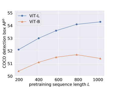
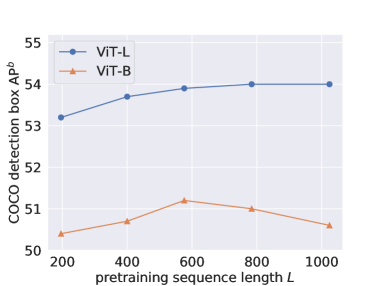
a) pre-training on COCO	b) pre-training on ImageNet-1K

Figure 3: Scaling trends of sequence length $L$ for pre-training on COCO or ImageNet-1K; and evaluating on COCO object detection with fixed transferring length. We make three observations: 1) Increasing sequence length $L$ generally leads to a healthy trend of better AP^b on COCO object detection. 2) The trend for ViT-L is better than ViT-B – the former continues to scale even at $L{=}1024$, whereas the latter saturates and even starts to decline after a certain point. 3) COCO pre-training benefits more from longer sequences than ImageNet-1K.

4.2 Scaling trends of sequence lengths

Given that sequence length $L{=}784$ improves downstream tasks as shown in Sec. 4.1, we next perform an in-depth study on the scaling trends of $L$. Specifically, we keep the patch size $p$ fixed as $16$, while varying the image size $I$ in $\left[224,320,384,448,512\right]$, corresponding to $L$ in $\left[196,400,576,784,1024\right]$. In addition to pre-training on COCO, we also include the ImageNet-1K dataset [11] as another pre-training source given its common use in previous work [19, 48]. For ImageNet-1K, we follow the standard setting and pre-train on its train split with 1,281,167 images under an 800-epoch schedule [19], which is roughly comparable to the total number of iterations in our COCO pre-training. To study how different ViTs behave with $L$, we also experiment with ViT-L [14], where we keep the same pre-training hyper-parameters as used in ViT-B (see Tab. 1).

For each pre-trained model, we report results on the COCO object detection task. For ViT-L, we again fine-tune for 50-epochs on the COCO annotations and follow the corresponding ViT-L fine-tuning hyper-parameters in [30].

The results are shown in Fig. 3. Overall, increasing the pre-training sequence length $L$ from $196$ to $1024$ generally brings continued benefits to the transfer performance on the COCO detection box AP^b. This is especially clear for the larger-sized ViT-L, while for the smaller ViT-B, AP^b saturates and even starts to decline after a certain sequence length for both COCO and ImageNet-1K pre-training. We suspect that ViT-L better scales to longer pre-training sequences than ViT-B because the former has a higher modeling capacity to handle a larger number of input image patches and learn rich features to represent the relationship among these patches (such as the part-whole relationship within an object or a scene, or the context co-occurrence relationship between visual components [32]). Given this observation, we hypothesize that it would be best to jointly scale the model parameters and the pre-training sequence length to learn stronger feature representations [39, 36].

In addition, comparing COCO pre-training in Fig. 3a) with ImageNet-1K pre-training in Fig. 3b), it can be seen that COCO pre-training benefits more from longer sequences: the former improves by more than $2$ AP points, whereas the latter by barely $1$ point. While not justified by controlled studies, we speculate this is because COCO images contain more objects and scene context on average than iconic ImageNet-1K images [32], and are therefore more friendly to longer sequences that capture these objects and their interactions.

4.3 More pre-training datasets

pre-training		COCO [32]			ImageNet-1K [11]			Open Images [25]			Places [50]
dataset		(241,690 images)			(1,281,167 images)			(1,743,042 images)			(1,803,460 images)
encoder	method	APb	APm	mIoU	APb	APm	mIoU	APb	APm	mIoU	APb	APm	mIoU
ViT-B	baseline	50.5	44.9	48.2	49.9	44.6	47.5	49.9	44.6	47.8	49.2	43.9	47.9
	ours	51.7	45.9	50.8	51.0	45.4	48.7	51.0	45.4	49.8	50.5	45.0	50.1
ViT-L	baseline	53.2	47.1	51.6	53.2	47.1	53.6	53.0	47.3	52.4	52.4	46.6	53.0
	ours	54.1	48.0	54.6	54.0	47.9	54.2	54.1	47.9	54.7	53.8	47.7	55.7

Table 3: More pre-training datasets with the MAE baseline ($L{=}196$) and our long sequence MAE ($L{=}784$), evaluated with fixed fine-tuning length on COCO (AP^b, AP^m) and ADE20K (mIoU). A longer sequence during pre-training consistently benefits all the experimental settings across different pre-training datasets, downstream transfers, and model sizes. Different pre-training sources also behave differently in terms of data efficiencies. For example, we find COCO pre-training to be highly effective for our tasks of interest, despite having fewer images.

Beyond COCO and ImageNet-1K, in this section we apply long-sequence MAE on more image sources for pre-training. Specifically, we choose two well-known datasets at a similar scale as ImageNet-1K, namely Open Images [25] and Places [50]. For Open Images, we pre-train on its training split with 1,743,042 images. For Places, we pre-train on the Places365-Standard training split with 1,803,460 images from 365 scene categories. For both ViT-B and ViT-L, we pre-train the baseline MAE and our long-sequence MAE for 800 epochs on Open Images and 600 epochs on Places, respectively. All other hyper-parameters and details are kept the same as default (Tab. 1).

Following Sec. 4.1, we evaluate all pre-trained models on COCO object detection, instance segmentation, and ADE20K semantic segmentation, where a fixed sequence length is used during fine-tuning for all evaluations. The results are summarized in Tab. 3. It can be seen that our long sequence pre-training ($L{=}784$) consistently outperforms the baseline setting ($L{=}196$) across all pre-training datasets and downstream tasks for both ViT-B and ViT-L. This confirms that long-sequence pre-training is a generic approach applicable and beneficial to various settings.

More interestingly, we also observe that different pre-training sources have different data efficiencies. Despite having only a fraction of images compared to other datasets (e.g., ${\raise 0.73193pt\hbox{$\scriptstyle\sim$}}1/5$ of ImageNet-1K), COCO pre-training is highly effective. For example, it achieves the highest mIoU ($50.8$) for ViT-B among all pre-training sources when transferring to ADE20K semantic segmentation, as well as on-par or better COCO detection and ADE20K segmentation accuracies than ImageNet-1K pre-training. As discussed in Sec. 4.2, we suspect this higher data efficiency is related to more scene-level images and a higher average number of objects in COCO, which benefits from a longer sequence. Furthermore, Places have a comparable number of images to Open Images, but the pre-trained ViT-L model on Places achieves the best results on ADE20K with $55.7$ mIoU – significantly outperforming the $53.3$ and $53.6$ mIoUs reported in BEiT [1] and MAE [19]. We attribute this to the rich variety of scenes in Places that helps learn better segmentation features and the close proximity in distribution to ADE20K [51].

4.4 COCO and LVIS with SimpleFPN

In this section, we further experiment with more downstream tasks and model architectures. We add LVIS [17] as another benchmark, and evaluate the pre-trained encoders by fine-tuning them with the state-of-the-art SimpleFPN [29] for plain ViT-based object detection and instance segmentation on both COCO and LVIS. Compared to the basic Mask R-CNN detector developed in [30], SimpleFPN [29] adopts a simpler and more efficient feature pyramid architecture [31], adapts the pre-trained backbone for detection with residual convolutions [21], and achieves a stronger performance.

Specifically, we pre-train the ViT models on both COCO and ImageNet-1K, using both the baseline MAE ($L=196$) and our long-sequence MAE ($L{=}784$). To match the setup in [29], we pre-train on ImageNet-1K for 1600 epochs. For COCO, we keep the 4,000-epoch schedule, as we find that more epochs do not give better performance. Then we fine-tune each pre-trained model separately on the COCO and LVIS bounding box and instance segmentation annotations with a fixed sequence length, and report their box AP^b and mask AP^m on both benchmarks.

The results are shown in Tab. 4, where models pre-trained with an increased sequence length again consistently outperform the baseline MAEs under both COCO and LVIS APs across different encoder architectures, despite all fine-tuning hyper-parameters are optimized for the baseline. In fact, the gains on LVIS are more salient than those on COCO, for example $+2.9$ in box AP^b from $43.3$ to $46.2$ with ViT-L pre-trained on COCO. When checking the detailed breakdown for classes with different frequencies, we find that long-sequence MAE helps more for long-tail classes. This further enhances our conclusion that long-sequence pre-training helps, this time generalizing to a new downstream task (LVIS) and the latest detector architecture (SimpleFPN).

pre-training dataset		COCO [32]				ImageNet-1K [11]
encoder	method	AP${}^{b}_{coco}$	AP${}^{m}_{coco}$	AP${}^{b}_{lvis}$	AP${}^{m}_{lvis}$	AP${}^{b}_{coco}$	AP${}^{m}_{coco}$	AP${}^{b}_{lvis}$	AP${}^{m}_{lvis}$
ViT-B	SimpleFPN [29]	–	–	–	–	51.6	45.9	40.2	38.2
	baseline	51.9	46.1	39.6	37.4	51.8	46.0	40.3	38.1
	ours	52.5	46.7	41.6	39.1	52.1	46.2	40.8	38.5
ViT-L	SimpleFPN [29]	–	–	–	–	55.6	49.2	46.0	43.4
	baseline	54.4	48.3	43.3	41.0	55.3	49.0	45.2	42.7
	ours	56.0	49.5	46.2	43.5	56.1	49.7	46.6	44.0

Table 4: COCO and LVIS with SimpleFPN for object detection and instance segmentation. For each model size (ViT-B and ViT-L), the first row contains the box AP^b and mask AP^m as reported in [29], for which the same pre-training recipe is used in our baseline. The second and third rows are results from our experiments. Our baseline can reproduce the results of [29] while our long-sequence MAE consistently outperforms the baseline, especially on LVIS.

pre-training dataset		COCO [32]	ImageNet-1K [11]
ViT-B	baseline	83.2	83.6
	ours	83.8	83.5
ViT-L	baseline	84.9	85.9
	ours	85.5	85.7

Table 5: We use ImageNet-1K classification as an additional downstream evaluation to complete our assessment of long-sequence pre-training for MAE. Unlike detection or segmentation tasks, the signal for classification is mixed, with noticeable gains from COCO pre-training, and no further benefit from ImageNet-1K. The same trend is observed for both ViT-B and ViT-L.

4.5 ImageNet-1K classification

So far we have mainly focused on the localization tasks that operate on scene-level images: object detection, instance segmentation, and semantic segmentation. To give a more complete picture of our long-sequence pre-training, we next extend the downstream evaluation to standard image classification on the ImageNet-1K dataset [11].

We conduct two sets of experiments. First, we use the standard classification setting and fix the input sequence length during fine-tuning ($I{=}224$, $p{=}16$, and $L{=}196$), given pre-trained models either from COCO (4,000-epoch) or ImageNet-1K (1600-epoch). Following the practice from previous sections, the pre-training is done either with or without long-sequence inputs, and for both ViT-B and ViT-L. Fine-tuning hyper-parameters and details strictly follow [19]. The results (in top-1 accuracy) are summarized in Tab. 5. Interestingly, the signal is mixed and is dependent on the pre-training dataset. With COCO, long-sequence pre-training offers substantial gains despite a reduced sequence length during supervised classification. In fact, for ViT-B, long-sequence MAE from COCO gives better ImageNet-1K accuracy ($83.8\%$) than any of our ImageNet-1K pre-trained MAEs, while using merely ${\raise 0.73193pt\hbox{$\scriptstyle\sim$}}1/5$ the number of images. On the other hand, ImageNet-1K pre-training with longer sequences does not bring immediate benefits for ImageNet classification if the fine-tuning length is fixed.

However, the above results do not mean long-sequence is not useful when dealing with ImageNet-1K images alone. On the contrary, we find sequence length is still playing a vital role in further driving the top-1 accuracy. In MAE, a state-of-the-art result ($87.8\%$) is achieved with input size $I=448$ [19], which effectively adopts a total sequence length of $L=1024$. To show that $L$ is more important than $I$, we pre-train a ViT-H model on ImageNet-1K for 800 epochs, with image size $I=224$ and patch size $p=7$, which also arrives at a total sequence length of $L{=}1024$. After pre-training, we fine-tune the model on ImageNet-1K with classification labels, following the ViT-H hyper-parameters and other details in [19]. For fine-tuning, we also stick to the image size $I=224$ and patch size $p=7$, and hence the same sequence length $L=1024$.

We evaluate the resulting model with standard $224{\times}224$ center-crop testing, and it gives a top-1 accuracy of $87.7\%$. This is comparable to MAE’s best result with the same model size, and is achieved with the same sequence length $L$, but without using a larger image size (or additional peripheral pixels [40]). This again shows that sequence length is the key to the performance boost, for both self-supervised pre-training and supervised classification as mentioned in [2].

5 Conclusion

In this work, we have explored long-sequence MAE pre-training, which has shown consistent improvements across various pre-training datasets and downstream benchmarks. The encouraging results suggest that sequence length is a viable axis for scaling, and has a potential compound effect [39] with the type of data used (e.g. scene-level [32, 50] vs. object-level [11]) and other important axes like model size. In contrast to model size, longer sequences during pre-training do not necessarily imply longer sequences during transferring, and indeed a fixed input size for evaluations is the analysis protocol we rigorously followed.

We have also established multiple MAE baselines on other image sources beyond ImageNet-1K, and showed that they can provide equivalent or better data efficiency and feature quality for relevant tasks. We hope this expansion can provide a more complete assessment of MAE.

One potential limitation of our work is that an increased sequence length inevitably increases the computational cost and thus the carbon footprint during pre-training. However, we believe this cost can be amortized by the various number of application possibilities from a single pre-training run; and justified by the performance gains without incurring extra costs during such transfers. While our current findings are mostly empirical, we hope they can aid future theoretical explanations and inspire more studies on this frontier.

Acknowledgments.

We are grateful to Ross Girshick, Kaiming He, and Alex Berg for helpful discussions on various ideas and experiments, and Yanghao Li and Hanzi Mao for their code base and examples of COCO and LVIS instance segmentation experiments before the public release, as well as Alexander Kirillov for the support on exploring other data sources for pre-training. We thank the Google TPU team for their Cloud TPU support.

pre-training splits		train2017			train+unlabeled2017
(COCO)		(118,287 images)			(241,690 images)
encoder	method	APb	APm	mIoU	APb	APm	mIoU
ViT-B	baseline	49.7	44.1	46.9	50.5	44.9	48.2
	ours	51.0	45.3	49.5	51.7	45.9	50.8
ViT-L	baseline	50.7	44.9	47.9	53.2	47.1	51.6
	ours	52.3	46.4	51.8	54.1	48.0	54.6

Table 6: Images from the COCO unlabeled2017 split roughly double the pre-training data size and greatly help downstream transfers to both COCO detection (AP^b, AP^m) and ADE20K segmentation (mIoU), evaluated under the same setting as in Tab. 3. We pre-train for 8,000 epochs on train2017 and 4,000 epochs on (train+unlabeled2017), which share roughly the same number of iterations and are near optimal for both pre-training data settings.

Appendix A Implementation details

Pre-training details.

We build our long-sequence pre-training upon the public MAE open-source repository implemented in PyTorch and adapt it to run on Cloud TPUs using PyTorch/XLA for our pre-training experiments. Our long-sequence pre-training mostly involves changing the image size $I$ and the patch size $p$ in the data loader and ViT model definition in this code base, as well as changing the sampling procedure for masked patch indices following our joint $m=2\times 2$ decoupled masking. Specifically, we move the mask index generation from the MAE network to the data loader to easily apply different masking strategies.

We follow the implementation details in the MAE open-source repository mentioned above in our pre-training experiments, except that we use a slightly smaller decoder (hidden size $384$ instead of $512$, and number of heads $12$ instead of $16$) in our ViT-B experiments throughout the paper for both the baseline MAE setting ($L=196$) and our long-sequence setting ($L=784$). This choice has a historical reason: In the early stage of the project, ViT-S (hidden size $384$) is among the encoders we used for efficient research explorations. For such a small model, maintaining a $512$ dimensional decoder offsets the asymmetric and efficient design of MAE as it leads to a heavier decoder that processes all the tokens. Therefore, our MAE design always keeps the decoder dimension half of the encoder dimension, and keeps the same number of heads to the encoder, for better adaptation to various-sized encoders. For ViT-B, it leads to a hidden size of $384$ and $12$ heads; for ViT-L, it is $512$ (same as the original MAE).

When reducing the decoder sequence length $L_{d}$ in LABEL:tab:ablate_enc_dec row 3, we insert a learned $2\times 2$ convolutional layer with stride 2 before the first decoder ViT block to down-sample $L_{d}$ from $28\times 28$ to $14\times 14$, which we find is slightly better than average pooling. In this case, we also reshape the target image (in the MAE reconstruction $\ell_{2}$ loss) to $14\times 14$ patches with doubled patch size $2p$ to matched the down-sampled $L_{d}$ and train the decoder to predict $2p\times 2p\times 3$ pixel targets.

Dataset details.

In our pre-training experiments on COCO, we find that pre-training on images from the union of train2017 and unlabeled2017 splits greatly improves the results over pre-training on train2017 alone, as detailed in Tab. 6. Notably, the former setting doubles the pre-training data size from 118,287 to 241,690. In addition to better transferring performance to ADE20K, the downstream COCO object detection and instance segmentation task itself (exclusively trained on the annotations from COCO train2017) also largely benefits from pre-training with the unlabeled2017 split. To our knowledge, this is one of the first use cases of the COCO unlabeled images that shows promising signals for object detection and segmentation. This confirms that the MAE pre-training helps downstream tasks through learning scalable (w.r.t. dataset size), unsupervised visual representations.

In our Open Images pre-training, since the dataset contains many high-resolution images, we first resize all the images to a long side of 640 pixels (following the image size of COCO) as a pre-processing step to reduce data loading overhead during pre-training. We use bicubic interpolation from the PIL library and save the resized images with a JPEG quality of 95, which gives better pre-training results than the default JPEG quality of 75 in the PIL library. When pre-training on all other datasets, we directly use the image files provided by these datasets.

References

- [1] Hangbo Bao, Li Dong, and Furu Wei. BEiT: BERT pre-training of image transformers. In ICLR, 2022.
- [2] Lucas Beyer, Xiaohua Zhai, and Alexander Kolesnikov. Better plain ViT baselines for ImageNet-1k. arXiv preprint arXiv:2205.01580, 2022.
- [3] Zhaowei Cai and Nuno Vasconcelos. Cascade R-CNN: Delving into high quality object detection. In CVPR, 2018.
- [4] Mathilde Caron, Hugo Touvron, Ishan Misra, Hervé Jégou, Julien Mairal, Piotr Bojanowski, and Armand Joulin. Emerging properties in self-supervised vision transformers. In ICCV, 2021.
- [5] Liang-Chieh Chen, George Papandreou, Iasonas Kokkinos, Kevin Murphy, and Alan L Yuille. DeepLab: Semantic image segmentation with deep convolutional nets, atrous convolution, and fully connected CRFs. TPAMI, 2017.
- [6] Mark Chen, Alec Radford, Rewon Child, Jeffrey Wu, Heewoo Jun, David Luan, and Ilya Sutskever. Generative pretraining from pixels. In ICML, 2020.
- [7] Ting Chen, Simon Kornblith, Mohammad Norouzi, and Geoffrey Hinton. A simple framework for contrastive learning of visual representations. In ICML, 2020.
- [8] Wuyang Chen, Xianzhi Du, Fan Yang, Lucas Beyer, Xiaohua Zhai, Tsung-Yi Lin, Huizhong Chen, Jing Li, Xiaodan Song, Zhangyang Wang, et al. A simple single-scale vision transformer for object localization and instance segmentation. arXiv preprint arXiv:2112.09747, 2021.
- [9] Xiaokang Chen, Mingyu Ding, Xiaodi Wang, Ying Xin, Shentong Mo, Yunhao Wang, Shumin Han, Ping Luo, Gang Zeng, and Jingdong Wang. Context autoencoder for self-supervised representation learning. arXiv preprint arXiv:2202.03026, 2022.
- [10] Xinlei Chen, Saining Xie, and Kaiming He. An empirical study of training self-supervised Vision Transformers. In ICCV, 2021.
- [11] Jia Deng, Wei Dong, Richard Socher, Li-Jia Li, Kai Li, and Li Fei-Fei. ImageNet: A large-scale hierarchical image database. In CVPR, 2009.
- [12] Jacob Devlin, Ming-Wei Chang, Kenton Lee, and Kristina Toutanova. BERT: Pre-training of deep bidirectional transformers for language understanding. In NAACL, 2019.
- [13] Xiaoyi Dong, Jianmin Bao, Ting Zhang, Dongdong Chen, Weiming Zhang, Lu Yuan, Dong Chen, Fang Wen, and Nenghai Yu. Peco: Perceptual codebook for bert pre-training of vision transformers. arXiv preprint arXiv:2111.12710, 2021.
- [14] Alexey Dosovitskiy, Lucas Beyer, Alexander Kolesnikov, Dirk Weissenborn, Xiaohua Zhai, Thomas Unterthiner, Mostafa Dehghani, Matthias Minderer, Georg Heigold, Sylvain Gelly, Jakob Uszkoreit, and Neil Houlsby. An image is worth 16x16 words: Transformers for image recognition at scale. In ICLR, 2021.
- [15] Alaaeldin El-Nouby, Gautier Izacard, Hugo Touvron, Ivan Laptev, Hervé Jegou, and Edouard Grave. Are large-scale datasets necessary for self-supervised pre-training? arXiv preprint arXiv:2112.10740, 2021.
- [16] Golnaz Ghiasi, Yin Cui, Aravind Srinivas, Rui Qian, Tsung-Yi Lin, Ekin D Cubuk, Quoc V Le, and Barret Zoph. Simple copy-paste is a strong data augmentation method for instance segmentation. In CVPR, 2021.
- [17] Agrim Gupta, Piotr Dollar, and Ross Girshick. LVIS: A dataset for large vocabulary instance segmentation. In CVPR, 2019.
- [18] Trevor Hastie, Robert Tibshirani, Jerome H Friedman, and Jerome H Friedman. The elements of statistical learning: data mining, inference, and prediction. Springer, 2009.
- [19] Kaiming He, Xinlei Chen, Saining Xie, Yanghao Li, Piotr Dollár, and Ross Girshick. Masked autoencoders are scalable vision learners. In CVPR, 2022.
- [20] Kaiming He, Georgia Gkioxari, Piotr Dollár, and Ross Girshick. Mask R-CNN. In ICCV, 2017.
- [21] Kaiming He, Xiangyu Zhang, Shaoqing Ren, and Jian Sun. Deep residual learning for image recognition. In CVPR, 2016.
- [22] Geoffrey Hinton, Oriol Vinyals, Jeff Dean, et al. Distilling the knowledge in a neural network. arXiv preprint arXiv:1503.02531, 2015.
- [23] Huaizu Jiang, Ishan Misra, Marcus Rohrbach, Erik Learned-Miller, and Xinlei Chen. In defense of grid features for visual question answering. In CVPR, 2020.
- [24] Alex Krizhevsky, Ilya Sutskever, and Geoff Hinton. Imagenet classification with deep convolutional neural networks. In NeurIPS, 2012.
- [25] Alina Kuznetsova, Hassan Rom, Neil Alldrin, Jasper Uijlings, Ivan Krasin, Jordi Pont-Tuset, Shahab Kamali, Stefan Popov, Matteo Malloci, Alexander Kolesnikov, et al. The open images dataset v4. IJCV, 2020.
- [26] Zhenzhong Lan, Mingda Chen, Sebastian Goodman, Kevin Gimpel, Piyush Sharma, and Radu Soricut. ALBERT: A lite bert for self-supervised learning of language representations. In ICLR, 2020.
- [27] Yann LeCun, Bernhard Boser, John S Denker, Donnie Henderson, Richard E Howard, Wayne Hubbard, and Lawrence D Jackel. Backpropagation applied to handwritten zip code recognition. Neural computation, 1989.
- [28] Chunyuan Li, Jianwei Yang, Pengchuan Zhang, Mei Gao, Bin Xiao, Xiyang Dai, Lu Yuan, and Jianfeng Gao. Efficient self-supervised vision transformers for representation learning. In ICLR, 2022.
- [29] Yanghao Li, Hanzi Mao, Ross Girshick, and Kaiming He. Exploring plain vision transformer backbones for object detection. arXiv preprint arXiv:2203.16527, 2022.
- [30] Yanghao Li, Saining Xie, Xinlei Chen, Piotr Dollar, Kaiming He, and Ross Girshick. Benchmarking detection transfer learning with vision transformers. arXiv preprint arXiv:2111.11429, 2021.
- [31] Tsung-Yi Lin, Piotr Dollár, Ross Girshick, Kaiming He, Bharath Hariharan, and Serge Belongie. Feature pyramid networks for object detection. In CVPR, 2017.
- [32] Tsung-Yi Lin, Michael Maire, Serge Belongie, James Hays, Pietro Perona, Deva Ramanan, Piotr Dollár, and C Lawrence Zitnick. Microsoft COCO: Common objects in context. In ECCV, 2014.
- [33] Hao Liu, Xinghua Jiang, Xin Li, Antai Guo, Deqiang Jiang, and Bo Ren. The devil is in the frequency: Geminated gestalt autoencoder for self-supervised visual pre-training. arXiv preprint arXiv:2204.08227, 2022.
- [34] Yinhan Liu, Myle Ott, Naman Goyal, Jingfei Du, Mandar Joshi, Danqi Chen, Omer Levy, Mike Lewis, Luke Zettlemoyer, and Veselin Stoyanov. Roberta: A robustly optimized bert pretraining approach. arXiv preprint arXiv:1907.11692, 2019.
- [35] Deepak Pathak, Philipp Krahenbuhl, Jeff Donahue, Trevor Darrell, and Alexei A Efros. Context encoders: Feature learning by inpainting. In CVPR, 2016.
- [36] Ilija Radosavovic, Raj Prateek Kosaraju, Ross Girshick, Kaiming He, and Piotr Dollár. Designing network design spaces. In CVPR, 2020.
- [37] Shaoqing Ren, Kaiming He, Ross Girshick, and Jian Sun. Faster R-CNN: Towards real-time object detection with region proposal networks. In NeurIPS, 2015.
- [38] Olaf Ronneberger, Philipp Fischer, and Thomas Brox. U-net: Convolutional networks for biomedical image segmentation. In MICCAI, 2015.
- [39] Mingxing Tan and Quoc Le. Efficientnet: Rethinking model scaling for convolutional neural networks. In ICML, 2019.
- [40] Hugo Touvron, Matthieu Cord, Matthijs Douze, Francisco Massa, Alexandre Sablayrolles, and Hervé Jégou. Training data-efficient image transformers & distillation through attention. In ICML, 2021.
- [41] Ashish Vaswani, Noam Shazeer, Niki Parmar, Jakob Uszkoreit, Llion Jones, Aidan N Gomez, Lukasz Kaiser, and Illia Polosukhin. Attention is all you need. In NeurIPS, 2017.
- [42] Pascal Vincent, Hugo Larochelle, Yoshua Bengio, and Pierre-Antoine Manzagol. Extracting and composing robust features with denoising autoencoders. In ICML, 2008.
- [43] Pascal Vincent, Hugo Larochelle, Isabelle Lajoie, Yoshua Bengio, Pierre-Antoine Manzagol, and Léon Bottou. Stacked denoising autoencoders: Learning useful representations in a deep network with a local denoising criterion. JMLR, 2010.
- [44] Jingdong Wang, Ke Sun, Tianheng Cheng, Borui Jiang, Chaorui Deng, Yang Zhao, Dong Liu, Yadong Mu, Mingkui Tan, Xinggang Wang, et al. Deep high-resolution representation learning for visual recognition. TPAMI, 2020.
- [45] Sinong Wang, Belinda Z Li, Madian Khabsa, Han Fang, and Hao Ma. Linformer: Self-attention with linear complexity. arXiv preprint arXiv:2006.04768, 2020.
- [46] Chen Wei, Haoqi Fan, Saining Xie, Chao-Yuan Wu, Alan Yuille, and Christoph Feichtenhofer. Masked feature prediction for self-supervised visual pre-training. In CVPR, 2022.
- [47] Tete Xiao, Yingcheng Liu, Bolei Zhou, Yuning Jiang, and Jian Sun. Unified perceptual parsing for scene understanding. In ECCV, 2018.
- [48] Zhenda Xie, Zheng Zhang, Yue Cao, Yutong Lin, Jianmin Bao, Zhuliang Yao, Qi Dai, and Han Hu. SimMIM: A simple framework for masked image modeling. arXiv preprint arXiv:2111.09886, 2021.
- [49] Fisher Yu and Vladlen Koltun. Multi-scale context aggregation by dilated convolutions. In ICLR, 2016.
- [50] Bolei Zhou, Agata Lapedriza, Aditya Khosla, Aude Oliva, and Antonio Torralba. Places: A 10 million image database for scene recognition. TPAMI, 2017.
- [51] Bolei Zhou, Hang Zhao, Xavier Puig, Tete Xiao, Sanja Fidler, Adela Barriuso, and Antonio Torralba. Semantic understanding of scenes through the ADE20K dataset. IJCV, 2019.
- [52] Jinghao Zhou, Chen Wei, Huiyu Wang, Wei Shen, Cihang Xie, Alan Yuille, and Tao Kong. iBOT: Image bert pre-training with online tokenizer. In ICLR, 2022.
- [53] Xizhou Zhu, Han Hu, Stephen Lin, and Jifeng Dai. Deformable convnets v2: More deformable, better results. In CVPR, 2019.