Projected Hybrid Density Functionals: Method and Application to Core Electron Ionization

Abstract

This work presents a new class of hybrid density functional theory (DFT) approximations, incorporating nonlocal exact exchange in predefined states such as core atomic orbitals (AOs). These projected hybrid density functionals are a flexible generalization of range-separated hybrids. This work derives projected hybrids using the Adiabatic Projection formalism. One projects the electron-electron interaction operator onto the chosen predefined states, reintroduces the projected operator into the noninteracting Kohn-Sham reference system, and introduces a density functional approximation for the remaining electron-electron interactions. Projected hybrids are readily implemented existing density functional codes, requiring only a projection of the one-electron density matrices and exchange operators entering existing routines. This work also presents a first application: a core-projected Perdew-Burke-Ernzerhof hybrid PBE0c70, in which the fraction of nonlocal exact exchange is increased from 25% to 70% in core AOs. Automatic selection of the projected AOs provides a black-box model chemistry appropriate for both core and valence electron properties. PBE0c70 predicts core orbital energies that accurately recover core-electron binding energies of second- and third-row elements, without degrading PBE0’s good performance for valence-electron properties.

I Introduction

Kohn-Sham density functional theory (DFT) is the most widely-used electronic structure approximation across chemistry, physics, and materials science.Verma2020 DFT models a system of interacting electrons in terms of a reference system of noninteracting Fermions, corrected by a mean-field (Hartree) electron repulsion and an exchange-correlation (XC) density functional incorporating all many-body effects.Janesko2021 Standard approxmations to the XC functional can capture important aspects of covalent bonding, at the expense of delocalization and self-interaction errors that lead to overbinding and over-delocalization.MoriSanchez2008 ; Perdew2017 Hybrid XC approximations mitigate these effects by including a fraction of nonlocal exact exchange, effectively reintroducing part of the electron-electron interaction into the reference system.Toulouse2009 However, introducing a fixed fraction of the entire electron-electron interaction leads to pervasive and resilient zero-sum tradeoffs between underbinding and over-delocalization.Ruzsinszky2006 ; Janesko2017 ; Janesko2021

The generalized range-separated adiabatic connection provides a way to optimize these tradeoffs.Savin1988 ; Savin1995 ; Leininger1997 ; Yang1998 ; Toulouse2004 ; Fromager2007 ; Toulouse2009 ; Savin2020 ; Pernal2021 This approach separates the electron-electron interaction operator $\hat{V}_{ee}$ into short-range and long-range pieces, for example

$$\hat{V}_{ee} = \sum_{i>j}\frac{1}{r_{ij}}\ =\ \sum_{i>j}\frac{{\textrm{ erf}}\left(\mu r_{ij}\right)}{r_{ij}}+\frac{{\textrm{ erfc}}\left(\mu r_{ij}\right)}{r_{ij}},$$

$$= \hat{V}^{LR}_{ee}+\hat{V}^{SR}_{ee}.$$

Part of the interaction, typically the long-range part, is reintroduced into the noninteracting reference system. The Hohenberg-Kohn theorems ensure that the real system’s ground-state energy and density can be obtained from an exact wavefunction calculation on the long-range-interacting reference system, corrected by a density functional for the remaining short-range Hartree-exchange-correlation energy. By relying on approximate XC functionals for only part of the electron-electron interaction, these approaches can provide beyond-zero-sum accuracy for certain properties, without the expense of a correlated wavefunction calculation on the real system.Pernal2021 Several groups have explored different approximations for the long-range-interacting reference system wavefunction, including coupled-cluster theory,Goll2005 multireference approaches,Fromager2007 ; Fromager2010 the density matrix renormalization group,Hedegaard2015 and the random phase approximation.Janesko2009b

Range-separated hybrids are an especially widely adopted approach.Henderson2008a These methods approximate the reference system wavefunction as a single Slater determinant, corrected by a density functional for full-range correlation.Toulouse2009 The development of range-separated exchange functionalsIikura2001 ; Ernzerhof1998 has enabled broad adoption of range-separated hybrids. Long-range-corrected (LC) hybrids introduce the long-range interaction into the reference system, and are widely adopted for Rydberg and charge-transfer excited states, noncovalent interactions, and more.Dreuw2003 ; Hedegaard2013 ; Rohrdanz2009 Screeneed hybrids introduce the short-range interaction into the reference system, and are widely adopted for semiconductors, metal oxides, and core excitations.Heyd2003 ; Wang2020 However, introducing a fixed range separation $\mu$ and fixed fraction of the short- and long-range interactions leaves remaining zero-sum tradeoffs.Janesko2017 Recent efforts to treat these tradeoffs include system-dependent range separation,Stein2009 ; Koerzdoerfer2014 local range separation,Krukau2008 range separations parameterized to particular properties,Besley2009 and other approximations reviewed in ref 2.

I.1 Adiabatic Projection

The Adiabatic Projection approach generalizes the range-separated adiabatic connection.Janesko2022 One replaces the range-separate interaction of eq I with a projected interaction defined by a set of two-electron projection operators $\{\hat{P}^{(2)}_{m}\}$:

$$\hat{V}^{P}_{ee} = \sum_{m}c_{m}\sum_{i>j}\hat{P}^{(2)}_{m}(i,j)\frac{1}{r_{ij}}\hat{P}^{(2)}_{m}(i,j).$$ (2)

(The notation $\hat{P}_{m}^{(2)}(i,j)$ means that the operator acts on electrons $i$ and $j$.) One then reintroduces the projected interaction into the reference system. Just as for the range-separated adaibatic connection, the Hohenberg-Kohn theorems ensure that the real system’s exact ground-state energy and density can be obtained from an exact wavefunction calculation on the projected-interacting reference system, corrected by a formally exact density functional for the projected Hartree-exchange-correlation energy.

We have applied the Adiabatic Projection approach to several contemporary problems in DFT. Projecting onto one-electron states $\hat{P}^{(2)}_{m}=\left|\phi_{m}\phi_{m}\right>\left<\phi_{m}\phi_{m}\right|$, $\left<\vec{r}|\phi_{m}\right>=\phi_{m}(\vec{r})$ introduces only self-interaction into the reference system. Choosing those one-electron states as localized Kohn-Sham spin-orbitals, and approximating the projected XC functional in terms of the orbital densities, recovers the Perdew-Zunger self-interaction correction (PZSIC).Perdew1981 ; Janesko2022a Other choices of one-electron states provides connections between the PZSIC, the Hubbard model DFT+U, and Rung 3.5 approximations.Janesko2022b Projecting onto active spaces of multiple occupied and virtual orbitals, and treating the reference system with a complete active-space self-consistent field (CASSCF) wavefunction, generalizes the PZSIC into a wavefunction-in-DFT approach.Janesko2022a

I.2 Projected hybrids

This work introduces projected hybrid density functionals inspired by range-separated hybrids. One projects the electron-electron interaction onto predefined states such as core atomic orbitals (AOs), approximates the reference system wavefunction as a single Slater determinant, and combines a projected exchange functionalJanesko2022a with a full-range correlation functional. This flexible approach permits exact exchange admixture in chemically appropriate regions, requires minimal modification to existing codes, and (unlike active-space approaches) can be incorporated into “black-box” model chemistries.

I.3 DFT for core electron properties

This pilot study introduces a core-projected hybrid functional targeted to simulate core- and valence- electron properties. Core-electron spectroscopies probe the chemical environment of nuclei and give element-specific information on bonding and oxidation state. The growing availability of bright X-ray sources has led to increasing interest in core electron spectroscopies.Norman2018 DFT and time-dependent (TD-)DFT simulations are widely adopted to interpret core electron spectra.Besley2020 DFT orbital energies, generated from accurate Kohn-Sham or generalized Kohn-ShamSeidl1996 potentials, can accurately predict the vertical ionization potentials (IPs) of both core and valence electrons.Chong2002 ; Bellafont2015 ; Verma2012a (In this approach, the first ionization potential is modeled as the negative of the highest occupied molecular orbital energy IP=-$\epsilon_{HOMO}$, and core ionization potentials are modeled as the negative of core molecular orbital energies.) Accurate XC potentials and orbital energies are also important for linear response TD-DFT simulations of X-ray absorption spectra.Zhang2012 ; Verma2016

Self-interaction error significantly impacts DFT-predicted core electron properties. For second-row elements Li-Ne, the core orbital energies predicted by standard global hybrid functionals differ by tens of eV from experimental K-edge core IPs.Tu2007 Comparable errors occur for TD-DFT predictions of core excitation energies.Nakata2006 ; Maier2016 Self-interaction errors are even worse for the more compact cores of third-row elements Na-Ar.Besley2021 Increasing the admixture of nonlocal exact exchange can improve predicted core IPs at the expense of a “zero-sum” degradation in valence electron properties.Fouda2020 Delta-self-consistent-field ($\Delta$SCF) approaches explicitly compute non-Aufbau core-ionized or core-excited state wavefunctions,Besley2009a providing a reduced impact of self-interaction error and a widely adopted practical solution.Norman2018 However, $\Delta$SCF approaches can suffer from difficulties converging the non-Aufbau states, require one SCF calcuation for each nucleus of interest in a large molecule, do not readily yield transition moments or vibronic couplings, and may still be significantly impacted by self-interaction error in heavier elements.Besley2021 The state-of-the-art for modeling X-ray fluorescence combines linear response TD-DFT with a constant shift taken from $\Delta$SCF calculations.Fouda2020 Mitigating the impact of self-interaction error on core elections, without degrading the treatment of valence electrons, could broaden the impact of inexpensive TD-DFT approaches.Maier2016

There has been significant interest in using self-interaction correction or exact exchange admixture to improve TD-DFT predictions of core electron spectroscopies. Tu and coworkers predicted core ionization potentials by applying a rescaled PZSIC to B3LYP-computed orbital energies.Tu2007 Several workers have developed range-separated hybrids that incorporate a large fraction of short-range nonlocal exchange. Hirao and coworkers modified their LCgau-BOP hybrid to include additional short-range nonlocal exchange, and reported improved TD-DFT core excitations for second-row atoms.Song2007 ; Song2008 Besley and coworkers reparameterized screened hybrid functionals to improve TD-DFT predictions of core excitations. They required different parameterizations for second-row and third-row atoms,Besley2009 which may be another manifestation of the zero-sum tradeoffs discussed above. Chai and coworkers introduced short- and long-range correction (SLC) hybrids including 100% nonlocal exchange at short and long range. SLC core orbital energies accurately predicted core ionization energies of second-row atoms, and TD-DFT with SLC functionals accurately predicted a range of core, valence, and charge-transfer excitations.Wang2016 Kaupp and coworkers showed that local hybrid functionals, incorporating a position-dependent admixture of exact exchange, provided balanced accuracy for TD-DFT predictions of the core excitations of second-row elements, along with valence, charge-transfer and Rydberg excitations.Maier2016 Nakata and coworkers introduced an orbital-dependent hybrid incorporating different fractions of HF exchange in different Kohn-Sham orbitals. The authors reported TD-DFT calcuations using the coupling operator technique of Roothaan, and found accurate core-excitation energies for second-row atoms.Nakata2006 This work was extended to a core-valence-Rydberg approach,Nakata2006a and is related to other orbital-dependent DFT methods.Ranasinghe2015

I.4 Core projected hybrids

This pilot study presents projected hybrids that incorporate additional nonlocal exchange in core AOs. Enhancing the Perdew-Burke-Ernzherhof global hybrid PBE0Perdew1996 ; Adamo1999 ; Scuseria1999 with 70% exact exchange in core AOs yields core molecular orbital (MO) energies that accurately predict second- and third-row $K$-edge ionization potentials, without a zero-sum degradation in valence electron properties. Numerical results are comparable to the core-valence hybrid of Nakata and coworkers,Nakata2006 without requiring the cumbersome coupling operator technique. The rest of this work presents a derivation of projected hybrids, details of the core-projected hybrid tested here, and numerical results.

II Derivation

This derivation of projected hybrid density functionals is based on published derivations of range-separated hybrids.Toulouse2009 In Kohn-Sham DFT, the exact ground-state energy of an $N$-electron system is expressed in terms of a noninteracting reference system and a density functional correction:

$$E = \min_{\Phi}\left(\left<\Phi|\hat{T}+\hat{V}_{ext}|\Phi\right>+E_{HXC}[\rho_{\Phi}]\right).$$ (3)

Here $\hat{T}$ and $\hat{V}_{ext}$ are operators for the the kinetic energy and external potential experienced by the reference system. $E_{HXC}[\rho]$ is the universal Hartree-exchange-correlation (HXC) density functional. Given the exact HXC functional, the reference system’s minimizing single-determinant wavefunction $\Phi$ yields ground-state energy $E$ and electron density $\rho_{\Phi}$ equal to the exact values.

Range-separated and projected hybrids respectively introduce the range-separated (eq I) and projected (eq 2) interactions into the reference system. The present work introduces a new choice of the projection in eq 2, based on an orthonormal set of $N_{P}$ single-particle states $\{\phi^{(P)}_{m}\}$ that are independent of the Kohn-Sham orbitals:

$$\hat{P}^{(2)} = \sum_{m,n}^{N_{P}}\left|\phi^{(P)}_{m}\phi^{(P)}_{n}\right>\left<\phi^{(P)}_{m}\phi^{(P)}_{n}\right|.$$ (4)

(For example, core-projected hybrids will choose $\{\phi^{(P)}_{m}\}$ by orthogonalizing the core AOs.) The ground-state energy is expressed as

$$E = \min_{\Psi^{LR}}\left(\left<\Psi^{LR}|\hat{T}+\hat{V}_{ext}+\hat{V}_{ee}^{LR}|\Psi^{LR}\right>+E_{HXC}^{SR}[\rho_{\Psi}^{LR}]\right),$$ (5)

in the generalized range-separated adiabatic connection and as

$$E = \min_{\Psi^{P}}\left(\left<\Psi^{P}|\hat{T}+\hat{V}_{ext}+\hat{V}_{ee}^{P}|\Psi^{P}\right>+E_{HXC}^{P}[\rho_{\Psi}^{P}]\right),$$ (6)

in the present work. Minimizing wavefunctions $\Psi^{LR}$ and $\Psi^{P}$ are generally multideterminant. Eq 5-6 yield the exact density and energy of the real system given the exact short-range and projected HXC functionals, respectively. The short-range HXC functional depends on the chosen range separation ($\mu$ in eq I), and the projected HXC functional depends on the projection $\hat{P}^{(2)}$ and thus on the chosen $\{\phi^{(P)}_{n}\}$.

Range-separated and projected hybrids are derived by restricting the minimizing wavefunctions in eq 5-6 to be single determinant:

$$E^{(0)}_{RSH} = \min_{\Phi^{LR}}\left(\left<\Phi^{LR}|\hat{T}+\hat{V}_{ext}+\hat{V}_{ee}^{LR}|\Phi^{LR}\right>+E_{HXC}^{SR}[\rho_{\Phi}^{LR}]\right),$$ (7)

$$E^{(0)}_{PH} = \min_{\Phi^{P}}\left(\left<\Phi^{P}|\hat{T}+\hat{V}_{ext}+\hat{V}_{ee}^{P}|\Phi^{P}\right>+E_{HXC}^{P}[\rho_{\Phi}^{P}]\right).$$ (8)

The minimizing determinants are given by the Euler-Lagrange equations:

$$\left(\hat{T}+\hat{V}_{ext}+\hat{J}-(\hat{K}-\hat{K}^{SR})+\hat{V}_{XC}^{SR}\right)\left|\Phi^{LR}\right> = \epsilon_{LR}\left|\Phi^{LR}\right>,$$ (9)

$$\left(\hat{T}+\hat{V}_{ext}+\hat{J}-(\hat{K}-\hat{K}^{P})+\hat{V}_{XC}^{P}\right)\left|\Phi^{P}\right> = \epsilon_{P}\left|\Phi^{P}\right>.$$ (10)

Here $\hat{J}$ is the Hartree potential, the sum of long-range and short-range terms (eq 9) or projected and unprojected terms (eq 10). $\hat{K},\hat{K}_{SR},\hat{K}_{P}$ are the full-range, short-range, and projected nonlocal exchange operators. $\epsilon_{LR}$ and $\epsilon_{P}$ are Lagrange multipliers for the normalization constraint.

The restriction to single determinants means that eq 7-8 do not yield the exact energy and density, even with the exact short-range or projected Hartree-exchange-correlation functionals. Nevertheless, they can be used as a reference to express the exact energy as $E=E_{RSH}+E_{C}^{LR}$ or $E_{PH}+E_{C}^{P^{\prime}}$. Conventional LC hybrids use a standard (full-range) correlation functional to model the sum of correlation in the long-range-interacting reference system $E_{C}^{LR}$, and the correlation piece of $E_{HXC}^{SR}$.Toulouse2009 This work uses a standard (unprojected) correlation functional to model the sum of correlation in the projected-interacting reference system, and the correlation piece of $E_{HXC}^{P}$. The hybrid functionals’ the total energies are

$$E_{RSH} = \min_{\Phi^{LR}}\left(\left<\Phi^{LR}|\hat{T}+\hat{V}_{ext}+\hat{V}_{ee}^{LR}|\Phi^{LR}\right>+U_{SR}[\rho_{\Phi}^{LR}]+E_{XSR}^{SL}[\rho_{\Phi}^{LR}]+E_{C}[\rho_{\Phi}^{LR}]\right),$$ (11)

for range-separated hybrids and

$$E^{(0)}_{PH} = \min_{\Phi^{P}}\left(\left<\Phi^{P}|\hat{T}+\hat{V}_{ext}+\hat{V}_{ee}^{P}|\Phi^{P}\right>+U_{P}[\rho_{\Phi}^{P}]+E_{XP}^{SL}[\rho_{\Phi}^{P}]+E_{C}^{SL}[\rho_{\Phi}^{P}]\right),$$ (12)

for projected hybrids.

Practical implementation of range-separated hybrid functionals requires explicit construction of range-separated semilocal exchange functionals $E_{XSR}^{SL}[\rho]$, based on models for the exchange hole. This is not the case for projected exchange functionals, where one may pass projected one-particle density matrices to unmodified semilocal exchange functionals. Ref 34 provides a detailed derivation of this approach, as a generalization of the Perdew-Zunger self-interaction correction.

III Implementation

This section presents the working equations for a projected hybrid’s generalized Kohn-Sham energy and potential. We consider the case of a core-projected hybrid calculation in an atomic orbital (AO) basis. The reference system’s single-determinant $N$-electron wavefunction $\left|\Phi^{P}\right>$ is made up of orthonormal one-electron spin-orbitals (MOs) $\{\left|\psi_{i\sigma}\right>\}$, each of which is expanded in a nonorthogonal basis set of $N_{basis}$ real AOs $\{\left|\chi_{\mu}\right>\}$. The overlap $\left<\chi_{\mu}|\chi_{\nu}\right>=S_{\mu\nu}$, where $S_{\mu\nu}$ is a matrix element of the $N_{basis}\times N_{basis}$ overlap matrix ${\bf{S}}$. The MOs are expanded as $\left|\psi_{i\sigma}\right>=\sum_{\mu}c_{i\sigma\mu}\left|\chi_{\mu}\right>$. The core-projected hybrid has $N_{core}\ll N_{basis}$ AOs are assigned as core AOs. The orthonormal projection states in eq 4 are denoted core states $\{\left|\phi^{(c)}_{m}\right>\}$, and are obtained by orthogonalizing the core AOs. Orthogonalization requires $\left(S^{(c)}\right)^{-1}_{\mu\nu}$, the matrix inverse of the $N_{core}\times N_{core}$ matrix of core AO overlaps.

Proceeding requires a one-electron projection operator $\hat{P}$ onto the orthogonalized core AOs. This operator’s representation in the full AO basis is

$$\hat{P} = \sum_{\mu\nu}\left|\chi_{\mu}\right>P_{\mu\nu}\left<\chi_{\nu}\right|.$$ (13)

Matrix element $P_{\mu\nu}$ of $N_{basis}\times N_{basis}$ matrix ${\bf{P}}$ equals $\left(S^{(c)}\right)^{-1}_{\mu\nu}$ when both $\chi_{\mu}$ and $\chi_{\nu}$ are core AOs, and equals zero elsewhere. This matrix obeys ${\bf{PSP}}={\bf{P}}$. The two-electron operator in eq 2 becomes $\hat{P}^{(2)}(i,j)=\hat{P}(i)\hat{P}(j)$, where $\hat{P}(i)$ denotes the projection of eq 13 acting on electron $i$. For any one-electron operator $\sum_{i}\hat{A}(i)$, the expectation value of the projected operator $\sum_{i}\hat{P}(i)\hat{A}(i)\hat{P}(i)$ becomes

$$\left<\Phi|\sum_{i}\hat{P}(i)\hat{A}(i)\hat{P}(i)|\Phi\right> = \sum_{i\sigma}\left<\psi_{i\sigma}\right|\left(\sum_{\mu\mu^{\prime}}\left|\chi_{\mu}\right>P_{\mu\mu^{\prime}}\left<\chi_{\mu^{\prime}}\right|\right)\hat{A}\left(\sum_{\nu^{\prime}\nu}\left|\chi_{\nu^{\prime}}\right>P_{\nu^{\prime}\nu}\left<\chi_{\nu}\right|\right)\left|\psi_{i\sigma}\right>,$$

$$= \sum_{i\sigma}\sum_{\mu\nu}c_{i\sigma\mu}^{*}A^{P}_{\mu\nu}c_{i\sigma\nu}.$$

This equation introduces matrix elements of the projected one-electron operator, which are defined as

$$A^{P}_{\mu\nu} = \sum_{\mu^{\prime}\mu"\nu^{\prime}\nu"}S_{\mu\mu^{\prime}}P_{\mu^{\prime}\mu"}A_{\mu"\nu"}P_{\nu"\nu^{\prime}}S_{\nu^{\prime}\nu}.$$ (15)

$A_{\mu\nu}=\left<\chi_{\mu}|\hat{A}|\chi_{\nu}\right>$ denotes matrix elements of the unprojected operator. The expectation value of the projected two-electron integral operator $\hat{V}_{ee}^{P}=\sum_{i\geq j}\hat{P}(i)\hat{P}(j)\hat{V}_{ee}(i,j)\hat{P}(i)\hat{P}(j)$ is

$$\left<\Phi|\hat{V}_{ee}^{P}|\Phi\right> = \frac{1}{2}\sum_{i\sigma}\sum_{j\sigma^{\prime}}\left<\psi_{i\sigma}\psi_{j\sigma^{\prime}}\right|\left(\sum_{\mu\nu\mu^{\prime}\nu^{\prime}}\left|\chi_{\mu}\chi_{\nu}\right>P_{\mu\mu^{\prime}}P_{\nu\nu^{\prime}}\left<\chi_{\mu^{\prime}}\chi_{\nu^{\prime}}\right|\right)\hat{V}_{ee}$$

$$\times \left(\sum_{\lambda^{\prime}\eta^{\prime}\lambda\eta}\left|\chi_{\lambda^{\prime}}\chi_{\eta^{\prime}}\right>P_{\lambda^{\prime}\lambda^{\prime}}P_{\eta^{\prime}\eta}\left<\chi_{\lambda}\chi_{\eta}\right|\right)\left(\left|\psi_{i\sigma}\psi_{j\sigma^{\prime}}\right>-\left|\psi_{j\sigma^{\prime}}\psi_{i\sigma}\right>\right),$$

$$= \frac{1}{2}\sum_{i\sigma}\sum_{j\sigma}c_{i\sigma\mu}^{*}c^{*}_{j\sigma^{\prime}\nu}\left<\mu\nu|\lambda\eta\right>^{P}\left(c_{i\sigma\lambda}c_{j\sigma^{\prime}\eta}-c_{j\sigma^{\prime}\lambda}c_{i\sigma\eta}\right).$$

The projected two-electron integrals are defined analogous to eq 15:

$$\left<\mu\nu|\lambda\eta\right>^{P} = \sum_{\mu^{\prime}\mu"\nu^{\prime}\nu"}\sum_{\lambda^{\prime}\lambda"\eta^{\prime}\eta"}S_{\mu\mu^{\prime}}P_{\mu^{\prime}\mu"}S_{\nu\nu^{\prime}}P_{\nu^{\prime}\nu"}\left<\mu"\nu"|\lambda"\eta"\right>P_{\lambda"\lambda^{\prime}}S_{\lambda^{\prime}\lambda}P_{\eta"\eta^{\prime}}S_{\eta^{\prime}\eta}$$ (17)

In practice, implementing projected hybrids does not require explicitly evaluating these projected AO-basis two-electron integrals. One only requires one-electron projections of density matrices and exchange operators. (However, the projected AO-basis two-electron integrals may be required for multi-determinant treatments of the projected interacting reference system, discussed in sec VI.) As shown in eq 10, the Hartree piece of eq III is combined with the remainder of the Hartree interaction from the projected Hartree-exchange-correlation density functional, yielding the usual ${\bf{J}}$ matrix. The exchange piece of eq III can be written as

$$E_{X}^{P} = -\frac{1}{2}\sum_{ij\sigma}\sum_{\mu\nu\lambda\eta}c^{*}_{i\sigma\mu}c^{*}_{j\sigma\nu}\left<\mu\nu|\lambda\eta\right>^{P}c_{j\sigma\lambda}c_{i\sigma\eta},$$

$$= -\frac{1}{2}\sum_{i\sigma}\sum_{\mu\eta}c^{*}_{i\sigma\mu}K^{P}_{\mu\eta}[\gamma^{P}_{\sigma}]c_{i\sigma\eta}.$$

Here $K^{P}_{\mu\eta}[\gamma^{P}_{\sigma}]$ denotes the projected (as in eq 15) nonlocal exact exchange operator constructed from projected density matrix $\gamma^{P}_{\sigma}$. Matrix elements of the the conventional AO-basis $\sigma$-spin one-particle density matrix are

$$\gamma_{\sigma\nu\lambda} = \sum_{i}c_{i\sigma\nu}c^{*}_{i\sigma\lambda}.$$ (19)

The projected density matrix is defined as

$$\gamma_{\sigma\nu\lambda}^{P} = \sum_{\nu^{\prime}\nu"\lambda^{\prime}\lambda"}P_{\nu\nu^{\prime}}S_{\nu^{\prime}\nu"}\gamma_{\sigma\nu"\lambda"}S_{\lambda"\lambda^{\prime}}P_{\lambda^{\prime}\lambda}.$$ (20)

(Note that the projected density matrix eq 20 is ${\bf{PS\gamma SP}}$, whereas the projected one-electron operator eq 15 is ${\bf{SPAPS}}$.) The unprojected exchange operator is constructed from the projected density matrix and unprojected AO-basis two-electron integrals as,

$$K_{\mu\eta}[\gamma^{P}] = \sum_{\nu"\lambda"}\left<\mu\nu"|\lambda"\eta\right>\gamma^{P}_{\sigma\nu"\lambda"}$$ (21)

Projecting this operator as in eq 15 recovers the first line of eq III.

The final step in the implementation involves the projected exchange functional, the analogue of the range-separated exchange functionals used in range-separated hybrids. As suggested above, we obtain the projected exchange functional by passing the projected density matrix to existing semilocal exchange functionals. We consider a standard $\sigma$-spin semilocal exchange functional

$$E_{X}^{SL}[\gamma_{\sigma}] = \int d^{3}\vec{r}\ e_{X}^{SL}\left[\rho_{\sigma}(\vec{r}),|\nabla\rho_{\sigma}(\vec{r})|\ldots\right],$$ (22)

$$\rho_{\sigma}(\vec{r}) = \sum_{\mu\nu}\chi_{\mu}(\vec{r})\gamma_{\mu\nu\sigma}\chi_{\nu}(\vec{r}).$$ (23)

We define the projected exchange functional as the difference between $E_{X}^{SL}$ evaluated with projected vs. unprojected density matrices. The total energy of a projected hybrid functional thus becomes

$$E = \sum_{ij\sigma}\sum_{\mu\nu}c_{i\sigma}^{*}\left(h_{\mu\nu}+\frac{1}{2}J_{\mu\nu}-\frac{1}{2}K^{P}_{\mu\nu}[\gamma^{P}_{\sigma}]\right)+E_{XC}^{SL}[\gamma]-\sum_{\sigma}E_{X}^{SL}[\gamma^{P}_{\sigma}]$$ (24)

Here $h_{\mu\nu}$ is a matrix element of the kinetic and external potential operators, $J_{\mu\nu}$ is a matrix element of the standard full-range Hartree potential, $E_{XC}^{SL}[\gamma]$ is a standard semilocal exchange-correlation functional evaluated on the full density matrix, and $E_{X}^{SL}[\gamma^{P}_{\sigma}]$ is the exchange piece of the semilocal functional (eq 22) evaluated on the projected density matrix of eq 20. The Fock-like matrix defined by $\partial E/\partial c_{i\mu\sigma}=\sum_{\nu}F_{\mu\nu\sigma}c_{i\nu\sigma}$, becomes (compare with eq 10)

$$F_{\mu\nu\sigma} = h_{\mu\nu}+J_{\mu\nu}+\left(V_{XC}^{SL}[\gamma]\right)_{\mu\nu\sigma}-K^{P}_{\mu\nu}[\gamma^{P}_{\sigma}]-\left(V_{X}^{SLP}[\gamma^{P}_{\sigma}]\right)_{\mu\nu}$$ (25)

Here the unprojected semilocal exchange operator is constructed from the projected density matrix in the usual way

$$\left(V_{X}^{SL}[\gamma^{P}_{\sigma}]\right)_{\mu\nu} = \int d^{3}\vec{r}\chi_{\mu}(\vec{r})\frac{\delta e_{X\sigma}^{SL}}{\delta\rho^{P}_{\sigma}(\vec{r})}\chi_{\nu}(\vec{r})+\ldots$$ (26)

Projecting this operator as in eq 15 recovers the $\left(V_{X}^{SLP}[\gamma^{P}_{\sigma}]\right)_{\mu\nu}$ in eq 25. Operationally, one constructs the projected AO-basis density matrix ${\bf{PS\gamma SP}}$, passes this to standard routines for constructing ${\bf{K}}$ and the semilocal exchange potential, then projects the operators (e.g. ${\bf{SPKPS}}$) before use. Because the projection states are independent of the MOs, self-consistent implementation merely requires these projections of one-particle density matrices and exchange operators.

IV Methods

This work uses an implementation of eq 24-25 into the PySCFSun2020 electronic structure package. The implementation is freely available online at github.com/bjanesko. Just as range-separated hybrids can include different fractions of short- and long-range exact exchange, the present implementation includes different fractions of projected exact exchange $\alpha_{c}$ and global exact exchange $\alpha_{0}$. This work adopts the notation "FcX", where "F" is a standard XC functional and "X" is the fraction of nonlocal exchange in core AOs. X="HF" is equivalent to X=100. For example, PBEcHF combines semilocal PBE with 100% HF exchange in AOs. Most benchmark calculations treat the PBE0c70 functional, combining PBE0 with 70% nonlocal exchange in core AOs ($\alpha_{0}=25\%,\alpha_{c}=70\%$).

In this pilot study, total energies and Fock-like matrices (eq 25) are computed from Hartree-Fock one-particle density matrices. Generalized Kohn-Sham orbital energies are obtained from a single diagonalization of the Fock-like matrices constructed from Hartree-Fock density matrices. Most calculations use the Perdew-Burke-ErnzerhofPerdew1996 (PBE) generalized gradient approximation, the PBE0 global hybrid incoporating 25% nonlocal exchange,Adamo1999 ; Scuseria1999 the PBEHH global hybrid incorporatng 50% nonlocal exchange, or the HFPBE combination of nonlocal exchange and PBE correlation. Test calculations treat the Becke-Lee-Yang-Parr (BLYP) GGA,Lee1988 ; Becke1988 the three-parameter global hybrid B3LYP,Becke1993a ; Cheeseman1996 the Tao-Perdew-Staroverov-Scuseria (TPSS) and Strongly Constrained and Appropriately Normed (SCAN) meta-GGAs,Tao2003 ; Sun2015 and the SCAN0 global hybrid. Other test calculations use the Gaussian 16 package,g16 and also include the M06L, M06, M06-2X, and M06-HF global hybrids,Zhao2006 ; Zhao2006a ; Zhao2006c the HSE06, N12SX, and MN12XS screened hybrids,Heyd2003 ; Peverati2012c and the LC-$\omega$PBE, $\omega$B97X-D, M11, Lc-BLYP, and CAM-B3LYP long-range-corrected hybrids.Vydrov2006a ; Yanai2004 ; Peverati2011 These calculations use post-HF total energies and self-consistent orbital eneriges. For the systems tested here, the two approaches methods are nearly identical: single-shot PBE with PySCF predicts CH₃Cl valence and core IP 7.14 and 2738.9 eV, self-consistent PBE with Gaussian 16 predicts valence and core IP 7.09 and 2739.7 eV. Calculations use several AO basis sets, including the 6-311++G(2d,2p) Pople-type basis set,Ditchfield1971 ; Hehre1972 the cc-pVnZ correlation-consistent basis sets,Dunning1989a the cc-pCVTZ and cc-pCVQZ basis sets designed for core electron properties, and the def2-SVP, def2-TZVP, def2-QZVP basis sets.Weigend2005 All molecular geometries are B3LYP/6-311++G(2d,2p) optimized.

This black-box study includes an automated choice of core AOs. Each second- and third-row element is assigned a cutoff kinetic energy as 1.4 times the kinetic energy from the most diffuse uncontracted core orbital in the STO-2G basis set. All s-type contrated AOs with kinetic energy above that cutoff are assigned to the core. For example, the STO-2G basis set for lithium atom includes a contracted 1s AO with exponents 6.16 and 1.10 au. The most diffuse exponent gives a kinetic energy $(3/2)1.10$ au and a cutoff $(1.4)(3/2)1.10$ au=2.3 au. All s-type contracted AOs centered on a Li atom $\{\chi_{\mu}^{Li}\}$, whose kinetic energy expectation value $\left<\chi_{\mu}^{Li}|\frac{1}{2}\nabla^{2}|\chi_{\mu}^{Li}\right>$ is above that threshold, are assigned as core. For the 6-311++G(2d,2p) basis set, this approach gives one core AOs for each second-row element and three core AOs for each third-row element.

V Results

V.1 Validation

Table 1 illustrates the overall performance of this approach, as well as the basis set dependence. The table shows valence, Cl core, and C core ionization potentials of CH₃Cl, computed from the corresponding generalized Kohn-Sham orbital energies. Calculations compare the PBEcHF core-projected hybrid (100% nonlocal exchange in core AOs) with PBE (no nonlocal exchange) and HFPBE (100% nonlocal exchange globally). As expected, the core-projected hybrid recovers the PBE valence IP to within 0.01 eV, and recovers the HFPBE core IP to within a few percent. Results are robust across basis sets, even as the number of core AOs changes from 2 to 11. This confirms that the projected hybrids and the core AO selection process perform as expected.

Table 1: Valence, C core, and Cl core ionization potentials of methylene chloride CH₃Cl (eV), computed as the negative of GKS orbital energies, evaluated in various basis sets.

		Valence			C atom core			Cl atom core
Basis	$N_{core}$	PBE	PBEcHF	HFPBE	PBE	PBEcHF	HFPBE	PBE	PBEcHF	HFPBE
STO-3G	2	4.94	4.94	11.64	267.3	303.5	303.7	2709.0	2814.1	2822.1
3-21G	2	7.09	7.09	13.15	270.5	307.2	306.9	2719.0	2826.7	2833.2
6-31G(d)	2	7.04	7.04	13.09	271.8	307.8	308.2	2738.4	2844.3	2852.7
6-311++G(2d,2p)	4	7.14	7.14	13.17	272.0	311.3	308.4	2738.9	2847.7	2853.2
cc-pvdz	4	6.95	6.95	13.03	272.0	307.7	308.4	2738.7	2847.6	2853.0
cc-pvtz	3	7.05	7.05	13.09	271.8	308.5	308.2	2738.8	2847.6	2853.1
cc-pcvtz	5	7.06	7.06	13.09	271.8	307.8	308.2	2738.8	2847.9	2853.1
cc-pvqz	5	7.09	7.09	13.11	271.8	308.5	308.2	2738.9	2847.8	2853.2
cc-pcvqz	11	7.09	7.09	13.11	271.8	307.8	308.2	2738.9	2847.3	2853.2
def2-svp	2	6.79	6.79	12.93	272.0	308.0	308.3	2737.5	2843.8	2851.8
def2-tzvp	3	7.06	7.06	13.08	271.8	299.9	308.2	2738.8	2848.2	2853.1
def2-qzvp	6	7.10	7.10	13.12	271.8	303.7	308.2	2738.9	2848.5	2853.2

Table 2 illustrates core-projected hybrid calculations using a variety of standard XC functionals. All core-projected hybrids use 100% nonlocal exchange in cores. For HFPBE, the unprojected and core-projected functionals are identical by construction. Otherwise, core projection increases the predicted core IP of second- and third-row atoms, without much affecting the HOMO energies. Whereas the unprojected functionals’ predicted core IP range over 30 eV for C and 110 eV for Cl, the core-projected functionals’ core IP are all within 6 eV of each other.

Table 2: Valence, C core, and Cl core ionization potentials of methylene chloride (eV), computed as the negative of GKS orbital energies, unmodified XC functional F vs. core-projected functional FcHF, 6-311++G(2d,2p) basis set.

	Valence		C atom core		Cl atom core
Functional F	F	FcHF	F	FcHF	F	FcHF
PBE	7.14	7.14	272.0	311.3	2738.9	2847.7
PBE0	8.64	8.64	281.1	310.6	2767.4	2849.0
PBEHH	10.15	10.15	290.2	309.8	2796.0	2850.4
HFPBE	13.17	13.17	308.4	308.4	2853.2	2853.2
BLYP	6.96	6.96	272.7	311.6	2740.7	2848.6
B3LYP	8.17	8.17	279.7	311.3	2762.4	2849.9
TPSS	7.33	7.33	274.8	310.7	2747.9	2848.6
SCAN	7.55	7.55	275.9	310.3	2753.6	2850.3
SCAN0	8.89	8.89	284.0	309.7	2778.4	2851.0

V.2 Benchmarks

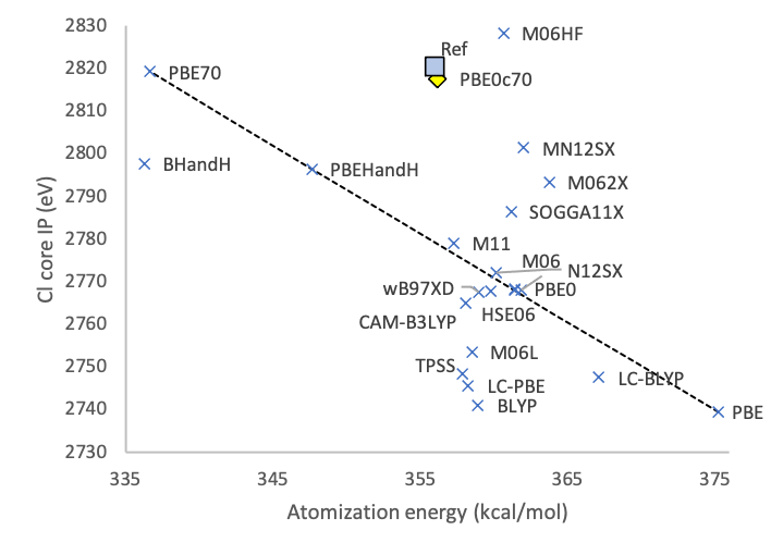
Figure 1: Computed atomization energy (abscissa) and Cl core IP (ordinate) of formyl chloride HCOCl. "X" denotes standard DFT functionals. Straight line denotes global hybrids of PBE including between 0 and 70% exact exchange. "Ref" is accurate reference values.

Figure 1 highlights the “zero-sum” trade-offs between predictions of valence and core properties, focusing on the atomization energy and core IP of formyl chloride HCOCl. Calculations use the def2-TZVP basis set. The figure shows the atomization energy on the abscissa, and the Cl core IP (negative of computed Cl 1s orbital energy) on the ordinate. Reference values are the 2820.6 eV core IP from ref 47, and a new CBS-QB3Montgomery1999 computed atomization energy 355.9 kcal/mol. Calculations compare core-projected PBE0c70 to a broad range of density functionals: semilocal PBE, BLYP, TPSS, M06L; global hybrid PBE0, PBEHandH, BHandH, M06-2X, M06-HF, and SOGGA11-X; and range-separated hybrids M11, $\omega$B97X-D, HSE06, LC-$\omega$PBE, LC-BLYP, CAM-B3LYP, N12-SX, MN12-SX. The straight line is results for PBE global hybrids including between 0 and 70% exact exchange.

The PBE global hybrid results clearly highlights the zero-sum tradeoff between valence and core properties. Introducing a fixed fraction of the entire nonlocal exchange interaction increases the predicted core IP, but also makes the predicted atomization energy less positive. PBE0 is near-optimal for the atomization energy, but underbinds the core electron. PBE70 is near-optimal for the core electron, but underestimates the chemical bond strengths. Most global hybrids lie close to this “zero-sum” line, accurately reproducing the atomization energy while underestimating the core IP. Long-range corrected hybrids tend to further underestimate the core IP. Screened hybrids MN12SX and N12SX, and the highly parameterized SOGGA11X, M06-2X, and M06-HF better approach the reference value. For this system, the core-projected hybrid PBE0c70 clearly provides the best agreement with the reference values employed.

The rest of this work presents a more detailed assessment of PBE0c70 on two data sets of core-electron ionization potentials. The first set is 33 $K$-shell ionization potentials of second-row atoms, from 14 small molecules, referenced to experiment.Tu2007 (In this dataset, “MBO” denotes 2-mercaptobenzoxazole.) The second set is 15 $K$-shell ionization potentials of third-row atoms, from 15 small molecules, referenced to nonrelativistic $\Delta$MP2 calculations.Besley2021 . Calculations use the 6-311++G(2d,2p) basis set and B3LYP/6-311++G(2d,2p) geometries.

Table 3 reports a validation of the valence properties predicted by core-projected PBE0c70. As the goal is to recover the underlying PBE0 global hybrid, mean absolute deviations MAD are referenced to PBE0. Gratifyingly, PBE0c70 gives ionization potentials within 0.01 eV of PBE0, and atomization energies within 1 kcal/mol of PBE0. Much larger deviations in valence properties are seen for the PBE70 global hybrid.

Table 3: Valence ionization potentials IP (eV) and atomization energies AE (kcal/mol), referenced to PBE0.

	IP			AE
Molecule	PBE0	PBE0c70	PBE70	PBE0	PBE0c70	PBE70
CO	11.21	11.21	14.21	251.6	251.4	231.4
H2O	8.93	8.93	12.64	224.9	224.9	213.9
CH4	11.13	11.13	14.01	413.6	413.3	412.4
CH3CN	9.75	9.75	12.23	294.7	294.0	268.9
CH3COOH	8.16	8.16	11.53	792.1	791.4	761.6
Glycine	7.64	7.64	10.59	956.1	955.3	915.6
MBO	6.71	6.71	8.54	1734.5	1731.8	1666.5
PhCH3	7.26	7.26	8.97	1666.1	1663.8	1632.9
PhNH2	6.24	6.24	8.1	1542.7	1540.5	1500.8
PhOH	6.83	6.83	8.72	1472.2	1470.1	1429.0
PhF	7.57	7.57	9.42	1380.4	1378.4	1339.8
C2H2	8.73	8.73	10.96	399.7	399.0	384.7
C2H4	8.17	8.17	10.2	557.6	557.0	548.7
C2H6	9.74	9.74	12.49	704.8	704.1	701.8
AlH3	8.61	8.61	11	197.0	196.2	203.4
AlH2Cl	8.75	8.75	11.24	217.8	216.9	221.9
AlH2F	8.89	8.89	11.43	259.4	258.5	257.7
SiH4	9.99	9.99	12.49	300.5	299.8	307.6
H3SiOH	8.62	8.62	11.58	422.5	421.7	419.6
H3SiCl	9.12	9.12	11.75	298.3	297.5	302.8
PH3	8.02	8.03	10.19	222.2	221.8	221.3
H3PO	7.8	7.8	10.95	295.0	294.4	283.0
H2POOH	8.06	8.06	11.22	410.7	410.0	388.7
CH3SH	7.1	7.1	9.45	456.7	456.2	451.5
H2CS	6.95	6.95	9.28	308.5	308.0	296.4
H2S	7.8	7.8	10.17	169.0	168.8	166.5
CH3Cl	8.64	8.64	11.36	385.1	384.7	380.7
HCOCl	9.28	9.28	12.25	354.6	354.2	330.5
HCl	9.69	9.69	12.45	99.5	99.4	97.7
MAD	—	0.00	2.55	—-	0.87	17.07

Tables 4-5 report second- and third-row core ionization potentials for the benchmark data sets. As in previous work, PBE0 core orbital energies are not an accurate predictor for core ionization potentials, giving MAD $>10$ eV for second-row atoms and $>40$ eV for third-row atoms. PBE70 significantly improves the core IP. Gratifyingly, PBE0c70 is nearly as accurate as PBE70, while maintaining PBE0 performance for valence electron properties.

Table 4: Core ionization potentials for second-row atoms (eV).

Molecule	Atom	Reference	PBE0	PBE0c70	PBE70
CO	O	542.1	525.9	549.6	548.4
	C	295.5	282.7	300.4	299.1
H2O	O	539.9	523.2	546.9	545.6
CH4	C	290.8	278.5	296.2	294.9
CH3CN	N	405.6	392.2	413.0	411.7
	CN	293.0	280.7	298.4	297.1
	CH3	292.4	280.5	298.1	296.9
CH3COOH	COOH	540.1	524.5	548.2	546.9
	COOH	538.4	522.8	546.5	545.2
	COOH	295.4	283.6	301.3	300.0
	CH3	291.6	279.7	297.3	296.1
Glycine	COOH	540.2	524.6	548.4	547.1
	COOH	538.4	522.9	546.7	545.4
	N	405.4	391.9	412.6	411.2
	COOH	295.3	283.6	301.3	300.0
	CH	295.2	280.6	298.3	297.0
MBO	O	540.6	525.6	549.3	548.0
	N	407.0	394.5	415.2	413.9
	CS	295.7	284.5	302.2	300.9
	CO	293.9	281.8	299.5	298.2
	CCN	293.0	281.5	299.2	297.9
	CCO	297.9	306.7	280.3	297.3
C6H5CH3	CH3	290.9	279.5	297.2	295.9
	CCH3	290.1	279.3	296.9	295.7
C6H5NH2	N	405.3	392.2	412.9	411.5
	CN	291.2	280.5	298.2	296.9
C6H5OH	O	538.9	523.9	547.6	546.3
	CO	292.0	281.3	298.9	297.6
C6H5F	F	693.3	674.3	701.0	699.8
	CF	292.9	281.9	299.6	298.3
C2H2	C	291.2	279.5	297.2	295.9
C2H4	C	290.7	279.2	296.9	295.6
C2H6	C	290.6	278.7	296.4	295.1
MAE		—-	13.0	7.0	5.3

Table 5: Core ionization potentials for third-row atoms (eV).

Molecule	Reference	PBE0	PBE0c70	PBE70
AlH3	1565.1	1528.5	1565.4	1566.8
AlH2Cl	1565.8	1530.0	1567.0	1568.3
AlH2F	1566.0	1529.4	1566.4	1567.7
SiH4	1843.2	1803.3	1843.2	1844.9
H3SiOH	1844.0	1804.2	1844.1	1845.7
H3SiCl	1844.3	1805.1	1845.1	1846.7
PH3	2145.8	2101.7	2144.6	2146.5
H3PO	2148.3	2104.7	2147.7	2149.6
H2POOH	2149.1	2105.7	2148.7	2150.6
CH3SH	2471.0	2422.8	2468.8	2471.0
H2CS	2471.2	2422.9	2468.9	2471.0
H2S	2471.7	2423.2	2469.2	2471.4
CH3Cl	2820.3	2767.4	2816.4	2818.9
HCOCl	2820.6	2768.4	2817.4	2819.8
HCl	2821.4	2768.2	2817.1	2819.6
MAE	—	44.1	1.6	1.3

VI Discussion

These results motivate further exploration of projected hybrids. Core-projected hybrids appear to be a promising choice for beyond-zero-sum TD-DFT simulations of X-ray absorbance and fluorescence of second- and third-row atoms, including vibronic structure, without the need for $\Delta$SCF corrections.Fouda2020 Other projections, for example projections onto metal $d$-electron states within a single unit cell, could provide connections between screened hybrid and DFT+U simulations of periodic systems. Going beyond the single-determinant approximation in eq 12 could provide an interesting alternative to active space selection and orbital localization in multiconfigurational methods.Janesko2022 ; Bao2019 ; Manni2014 Consider for example a calculation on a large organometallic complex known to possess multireference character in the metal $d$ electrons. Rather than choosing an active space of correlated MOs, one could project the metal atom $d$ AOs into the reference system, leaving only $\sim 10^{3}$ nonzero AO-basis two-electron integrals. Algorithms that account for this extreme sparsity of AO-basis integrals could potentially provide near-full-CI accuracy for the entire reference system, giving a “black-box” alternative to multireference wavefunction-in-DFT approaches.Sharma2021 Overall, the present results motivate further development of Adiabatic Projection hybrids, just as Refs 26 and 23 motivated broad adoption of screened and LC hybrids.

VII Acknowledgments

The author acknowledges the Texas Advanced Computing Center at the University of Texas at Austin for providing HPC resources that have contributed to the research results reported within this paper.

References

- (1) P. Verma and D. G. Truhlar, Status and challenges of density functional theory, Trends in Chemistry 2, 302 (2020).
- (2) B. G. Janesko, Replacing hybrid density functional theory: motivation and recent advances, Chem. Soc. Rev. (2021).
- (3) P. Mori-Sánchez, A. J. Cohen, and W. Yang, Localization and delocalization errors in density functional theory and implications for band-gap prediction, Phys. Rev. Lett. 100, 146401 (2008).
- (4) J. P. Perdew et al., Understanding band gaps of solids in generalized kohn–sham theory, Proc. Natl. Acad. Sci. 114, 2801 (2017).
- (5) J. Toulouse, I. C. Gerber, G. Jansen, A. Savin, and J. G. Ángyán, Adiabatic-connection fluctuation-dissipation density-functional theory based on range separation, Phys. Rev. Lett. 102, 096404 (2009).
- (6) A. Ruzsinszky, J. P. Perdew, G. I. Csonka, O. A. Vydrov, and G. E. Scuseria, Spurious fractional charge on dissociated atoms: Pervasive and resilient self-interaction error of common density functionals, J. Chem. Phys. 125, 194112 (2006).
- (7) B. G. Janesko, E. Proynov, J. Kong, G. Scalmani, and M. J. Frisch, Practical density functionals beyond the overdelocalization–underbinding zero-sum game, The Journal of Physical Chemistry Letters 8, 4314 (2017).
- (8) A. Savin, A combined density functional and configuration interaction method, Int. J. Quantum Chem. 34, 59 (1988).
- (9) A. Savin and H.-J. Flad, Density functionals for the yukawa electron-electron interaction, Int. J. Quantum Chem. 56, 327 (1995).
- (10) T. Leininger, H. Stoll, H.-J. Werner, and A. Savin, Combining long-range configuration interaction with short-range density functionals, Chem. Phys. Lett. 275, 151 (1997).
- (11) W. Yang, Generalized adiabatic connection in density functional theory, J. Chem. Phys. 109, 10107 (1998).
- (12) J. Toulouse, F. Colonna, and A. Savin, Long-range–short-range separation of the electron-electron interaction in density-functional theory, Phys. Rev. A 70, 062505 (2004).
- (13) E. Fromager, J. Toulouse, and H. J. A. Jensen, On the universality of the long-/short-range separation in multiconfigurational density-functional theory, J. Chem. Phys. 126, 074111 (2007).
- (14) A. Savin, Models and corrections: Range separation for electronic interaction—lessons from density functional theory, J. Chem. Phys. 153, 160901 (2020).
- (15) K. Pernal and M. Hapka, Range-separated multiconfigurational density functional theory methods, WIREs Computational Molecular Science 12 (2021).
- (16) E. Goll, H.-J. Werner, and H. Stoll, A short-range gradient-corrected density functional in long-range coupled-cluster calculations for rare gas dimers, Physical Chemistry Chemical Physics 7, 3917 (2005).
- (17) E. Fromager, R. Cimiraglia, and H. J. A. Jensen, Merging multireference perturbation and density-functional theories by means of range separation: Potential curves for be2, mg2, and ca2, Physical Review A 81, 024502 (2010).
- (18) E. D. Hedegaard, S. Knecht, J. S. Kielberg, H. J. A. Jensen, and M. Reiher, Density matrix renormalization group with efficient dynamical electron correlation through range separation, J. Chem. Phys. 142, 224108 (2015).
- (19) B. G. Janesko, T. M. Henderson, and G. E. Scuseria, Long-range-corrected hybrids including random phase approximation correlation, J. Chem. Phys. 130, 081105 (2009).
- (20) T. M. Henderson, B. G. Janesko, and G. E. Scuseria, Range separation and local hybridization in density functional theory, The Journal of Physical Chemistry A 112, 12530 (2008).
- (21) H. Iikura, T. Tsuneda, T. Yanai, and K. Hirao, A long-range correction scheme for generalized-gradient-approximation exchange functionals, J. Chem. Phys. 115, 3540 (2001).
- (22) M. Ernzerhof and J. P. Perdew, Generalized gradient approximation to the angle- and system-averaged exchange hole, J. Chem. Phys. 109, 3313 (1998).
- (23) A. Dreuw, J. L. Weisman, and M. Head-Gordon, Long-range charge-transfer excited states in time-dependent density functional theory require non-local exchange, J. Chem. Phys. 119, 2943 (2003).
- (24) E. D. Hedegaard, F. Heiden, S. Knecht, E. Fromager, and H. J. A. Jensen, Assessment of charge-transfer excitations with time-dependent, range-separated density functional theory based on long-range MP2 and multiconfigurational self-consistent field wave functions, The Journal of Chemical Physics 139, 184308 (2013).
- (25) M. A. Rohrdanz, K. M. Martins, and J. M. Herbert, A long-range-corrected density functional that performs well for both ground-state properties and time-dependent density functional theory excitation energies, including charge-transfer excited states, J. Chem. Phys. 130, 054112 (2009).
- (26) J. Heyd, G. E. Scuseria, and M. Ernzerhof, Hybrid functionals based on a screened Coulomb potential, J. Chem. Phys. 118, 8207 (2003).
- (27) Y. Wang et al., M06-sx screened-exchange density functional for chemistry and solid-state physics, Proc. Natl. Acad. Sci. 117, 2294 (2020).
- (28) T. Stein, L. Kronik, and R. Baer, Reliable prediction of charge transfer excitations in molecular complexes using time-dependent density functional theory, J. Am. Chem. Soc. 131, 2818 (2009).
- (29) T. Körzdörfer and J.-L. Brédas, Organic electronic materials: Recent advances in the DFT description of the ground and excited states using tuned range-separated hybrid functionals, Acc. Chem. Res. 47, 3284 (2014).
- (30) A. V. Krukau, G. E. Scuseria, J. P. Perdew, and A. Savin, Hybrid functionals with local range separation, J. Chem. Phys. 129, 124103 (2008).
- (31) N. A. Besley, M. J. G. Peach, and D. J. Tozer, Time-dependent density functional theory calculations of near-edge x-ray absorption fine structure with short-range corrected functionals, Physical Chemistry Chemical Physics 11, 10350 (2009).
- (32) B. G. Janesko and E. N. Brothers, Virtual experiments on real asphaltenes: Predicting properties using quantum chemical simulations of structures from non-contact atomic force microscopy, Energy & Fuels (2022).
- (33) J. P. Perdew and A. Zunger, Self-interaction correction to density-functional approximations for many-electron systems, Phys. Rev. B 23, 5048 (1981).
- (34) B. G. Janesko, Adiabatic projection: Bridging ab initio, density functional, semiempirical, and embedding approximations, J. Chem. Phys. 156, 014111 (2022).
- (35) B. G. Janesko, Systematically improvable generalization of self-interaction corrected density functional theory, The Journal of Physical Chemistry Letters 13, 5698 (2022).
- (36) P. Norman and A. Dreuw, Simulating x-ray spectroscopies and calculating core-excited states of molecules, Chemical Reviews 118, 7208 (2018).
- (37) N. A. Besley, Density functional theory based methods for the calculation of x-ray spectroscopy, Accounts of Chemical Research 53, 1306 (2020).
- (38) A. Seidl, A. Görling, P. Vogl, J. A. Majewski, and M. Levy, Generalized Kohn-Sham schemes and the band-gap problem, Phys. Rev. B 53, 3764 (1996).
- (39) D. P. Chong, O. V. Gritsenko, and E. J. Baerends, Interpretation of the kohn–sham orbital energies as approximate vertical ionization potentials, The Journal of Chemical Physics 116, 1760 (2002).
- (40) N. P. Bellafont, P. S. Bagus, and F. Illas, Prediction of core level binding energies in density functional theory: Rigorous definition of initial and final state contributions and implications on the physical meaning of kohn-sham energies, The Journal of Chemical Physics 142, 214102 (2015).
- (41) P. Verma and R. J. Bartlett, Increasing the applicability of density functional theory. III. do consistent kohn-sham density functional methods exist?, The Journal of Chemical Physics 137, 134102 (2012).
- (42) Y. Zhang, J. D. Biggs, D. Healion, N. Govind, and S. Mukamel, Core and valence excitations in resonant x-ray spectroscopy using restricted excitation window time-dependent density functional theory, The Journal of Chemical Physics 137, 194306 (2012).
- (43) P. Verma and R. J. Bartlett, Increasing the applicability of density functional theory. v. x-ray absorption spectra with ionization potential corrected exchange and correlation potentials, The Journal of Chemical Physics 145, 034108 (2016).
- (44) G. Tu, V. Carravetta, O. Vahtras, and H. gren, Core ionization potentials from self-interaction corrected kohn-sham orbital energies, J. Chem. Phys. 127, 174110 (2007).
- (45) A. Nakata, Y. Imamura, T. Otsuka, and H. Nakai, Time-dependent density functional theory calculations for core-excited states: Assessment of standard exchange-correlation functionals and development of a novel hybrid functional, The Journal of Chemical Physics 124, 094105 (2006).
- (46) T. M. Maier, H. Bahmann, A. V. Arbuznikov, and M. Kaupp, Validation of local hybrid functionals for TDDFT calculations of electronic excitation energies, J. Chem. Phys. 144, 074106 (2016).
- (47) N. A. Besley, Density functional theory calculations of core–electron binding energies at the k-edge of heavier elements, Journal of Chemical Theory and Computation 17, 3644 (2021).
- (48) A. A. E. Fouda and N. A. Besley, Improving the predictive quality of time-dependent density functional theory calculations of the x-ray emission spectroscopy of organic molecules, Journal of Computational Chemistry 41, 1081 (2020).
- (49) N. A. Besley, A. T. B. Gilbert, and P. M. W. Gill, Self-consistent-field calculations of core excited states, The Journal of Chemical Physics 130, 124308 (2009).
- (50) J.-W. Song, S. Tokura, T. Sato, M. A. Watson, and K. Hirao, An improved long-range corrected hybrid exchange-correlation functional including a short-range gaussian attenuation (LCgau-BOP), The Journal of Chemical Physics 127, 154109 (2007).
- (51) J.-W. Song, M. A. Watson, A. Nakata, and K. Hirao, Core-excitation energy calculations with a long-range corrected hybrid exchange-correlation functional including a short-range gaussian attenuation (LCgau-BOP), J. Chem. Phys. 129, 184113 (2008).
- (52) C.-W. Wang, K. Hui, and J.-D. Chai, Short- and long-range corrected hybrid density functionals with the d3 dispersion corrections, J. Chem. Phys. 145, 204101 (2016).
- (53) A. Nakata, Y. Imamura, and H. Nakai, Hybrid exchange-correlation functional for core, valence, and rydberg excitations: Core-valence-rydberg b3lyp, The Journal of Chemical Physics 125, 064109 (2006).
- (54) D. S. Ranasinghe, M. J. Frisch, and G. A. Petersson, A density functional for core-valence correlation energy, The Journal of Chemical Physics 143, 214111 (2015).
- (55) J. P. Perdew, K. Burke, and M. Ernzerhof, Generalized gradient approximation made simple, Phys. Rev. Lett. 77, 3865 (1996).
- (56) C. Adamo and V. Barone, Toward reliable density functional methods without adjustable parameters: The PBE0 model, J. Chem. Phys. 110, 6158 (1999).
- (57) G. E. Scuseria and P. Y. Ayala, Linear scaling coupled cluster and perturbation theories in the atomic orbital basis, J. Chem. Phys. 111, 8330 (1999).
- (58) Q. Sun et al., Recent developments in the PySCF program package, J. Chem. Phys. 153, 024109 (2020).
- (59) C. Lee, W. Yang, and R. G. Parr, Development of the colle-salvetti correlation-energy formula into a functional of the electron density, Phys. Rev. B 37, 785 (1988).
- (60) A. D. Becke, Density-functional exchange-energy approximation with correct asymptotic behavior, Phys. Rev. A 38, 3098 (1988).
- (61) A. D. Becke, Density-functional thermochemistry. III. the role of exact exchange, J. Chem. Phys. 98, 5648 (1993).
- (62) J. R. Cheeseman, G. W. Trucks, T. A. Keith, and M. J. Frisch, A comparison of models for calculating nuclear magnetic resonance shielding tensors, J. Chem. Phys. 104, 5497 (1996).
- (63) J. Tao, J. P. Perdew, V. N. Staroverov, and G. E. Scuseria, Climbing the density functional ladder: Nonempirical meta–generalized gradient approximation designed for molecules and solids, Phys. Rev. Lett. 91, 146401 (2003).
- (64) J. Sun, A. Ruzsinszky, and J. P. Perdew, Strongly constrained and appropriately normed semilocal density functional, Phys. Rev. Lett. 115, 036402 (2015).
- (65) Gaussian 16, Revision C.01, Frisch, M. J.; Trucks, G. W.; Schlegel, H. B.; Scuseria, G. E.; Robb, M. A.; Cheeseman, J. R.; Scalmani, G.; Barone, V.; Petersson, G. A.; Nakatsuji, H.; Li, X.; Caricato, M.; Marenich, A. V.; Bloino, J.; Janesko, B. G.; Gomperts, R.; Mennucci, B.; Hratchian, H. P.; Ortiz, J. V.; Izmaylov, A. F.; Sonnenberg, J. L.; Williams-Young, D.; Ding, F.; Lipparini, F.; Egidi, F.; Goings, J.; Peng, B.; Petrone, A.; Henderson, T.; Ranasinghe, D.; Zakrzewski, V. G.; Gao, J.; Rega, N.; Zheng, G.; Liang, W.; Hada, M.; Ehara, M.; Toyota, K.; Fukuda, R.; Hasegawa, J.; Ishida, M.; Nakajima, T.; Honda, Y.; Kitao, O.; Nakai, H.; Vreven, T.; Throssell, K.; Montgomery, J. A., Jr.; Peralta, J. E.; Ogliaro, F.; Bearpark, M. J.; Heyd, J. J.; Brothers, E. N.; Kudin, K. N.; Staroverov, V. N.; Keith, T. A.; Kobayashi, R.; Normand, J.; Raghavachari, K.; Rendell, A. P.; Burant, J. C.; Iyengar, S. S.; Tomasi, J.; Cossi, M.; Millam, J. M.; Klene, M.; Adamo, C.; Cammi, R.; Ochterski, J. W.; Martin, R. L.; Morokuma, K.; Farkas, O.; Foresman, J. B.; Fox, D. J. Gaussian, Inc., Wallingford CT, 2016.
- (66) Y. Zhao and D. G. Truhlar, A new local density functional for main-group thermochemistry, transition metal bonding, thermochemical kinetics, and noncovalent interactions, J. Chem. Phys. 125, 194101 (2006).
- (67) Y. Zhao and D. G. Truhlar, Density functionals for noncovalent interaction energies of biological importance, J. Chem. Theory Comput. 3, 289 (2006).
- (68) Y. Zhao and D. G. Truhlar, Density functional for spectroscopy: No long-range self-interaction error, good performance for rydberg and charge-transfer states, and better performance on average than b3lyp for ground states, J. Phys. Chem. A 110, 13126 (2006).
- (69) R. Peverati and D. G. Truhlar, Screened-exchange density functionals with broad accuracy for chemistry and solid-state physics, Physical Chemistry Chemical Physics 14, 16187 (2012).
- (70) O. A. Vydrov and G. E. Scuseria, Assessment of a long-range corrected hybrid functional, J. Chem. Phys. 125, 234109 (2006).
- (71) T. Yanai, D. P. Tew, and N. C. Handy, A new hybrid exchange–correlation functional using the coulomb-attenuating method (CAM-b3lyp), Chem. Phys. Lett. 393, 51 (2004).
- (72) R. Peverati and D. G. Truhlar, Improving the accuracy of hybrid meta-gga density functionals by range separation, The Journal of Physical Chemistry Letters 2, 2810 (2011).
- (73) R. Ditchfield, W. J. Hehre, and J. A. Pople, Self-consistent molecular-orbital methods. IX. an extended gaussian-type basis for molecular-orbital studies of organic molecules, J. Chem. Phys. 54, 724 (1971).
- (74) W. J. Hehre, R. Ditchfield, and J. A. Pople, Self—consistent molecular orbital methods. XII. further extensions of gaussian—type basis sets for use in molecular orbital studies of organic molecules, J. Chem. Phys. 56, 2257 (1972).
- (75) T. H. Dunning, Gaussian basis sets for use in correlated molecular calculations. i. the atoms boron through neon and hydrogen, J. Chem. Phys. 90, 1007 (1989).
- (76) F. Weigend and R. Ahlrichs, Balanced basis sets of split valence, triple zeta valence and quadruple zeta valence quality for H to Rn: Design and assessment of accuracy, Phys. Chem. Chem. Phys. 7, 3297 (2005).
- (77) J. A. Montgomery, M. J. Frisch, J. W. Ochterski, and G. A. Petersson, A complete basis set model chemistry. VI. use of density functional geometries and frequencies, J. Chem. Phys. 110, 2822 (1999).
- (78) J. J. Bao and D. G. Truhlar, Automatic active space selection for calculating electronic excitation energies based on high-spin unrestricted hartree–fock orbitals, Journal of Chemical Theory and Computation 15, 5308 (2019).
- (79) G. L. Manni et al., Multiconfiguration pair-density functional theory, J. Chem. Theory Comput. 10, 3669 (2014).
- (80) P. Sharma, J. J. Bao, D. G. Truhlar, and L. Gagliardi, Multiconfiguration pair-density functional theory, Ann. Rev. Phys. Chem. 72, 541 (2021).