CUF: Continuous Upsampling Filters

Abstract

Neural fields have rapidly been adopted for representing 3D signals, but their application to more classical 2D image-processing has been relatively limited. In this paper, we consider one of the most important operations in image processing: upsampling. In deep learning, learnable upsampling layers have extensively been used for single image super-resolution. We propose to parameterize upsampling kernels as neural fields. This parameterization leads to a compact architecture that obtains a 40-fold reduction in the number of parameters when compared with competing arbitrary-scale super-resolution architectures. When upsampling images of size 256x256 we show that our architecture is 2x-10x more efficient than competing arbitrary-scale super-resolution architectures, and more efficient than sub-pixel convolutions when instantiated to a single-scale model. In the general setting, these gains grow polynomially with the square of the target scale. We validate our method on standard benchmarks showing such efficiency gains can be achieved without sacrifices in super-resolution performance.

1 Introduction

Neural-fields represent signals with coordinate-based neural-networks. They have found application in a multitude of areas including 3D reconstruction[24], novel-view synthesis [30], convolutions [14], and many others [35].

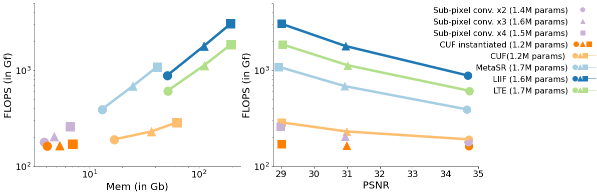
Figure 1: We report (left) memory and FLOPs for upsampling an $256\times 256$ image by different scale factors ($2\times$,$3\times$,$4\times$) using integer scale upsamplers (Sub-Pixel Convolution [29] and CUF-instantiated) and arbitrary-scale upsamplers (Meta-SR [16], LIIF [6], LTE [19] and CUF), but the same encoder backbone (EDSR-baseline [21]); and (right) the relationship between each upsampler FLOPS and PSNR performance on DIV2k dataset. Our arbitrary scale model is significantly lighter than other methods in the same class (i.e. continuous super-res). Further, when instantiated for integer scale factors, our upsampler is even-more efficient than sub-pixel convolutions [29].

Recent research has investigated the use of neural fields in the context of single image super-resolution [6, 19]. These models are based on multi-layer perceptrons conditioned on latent representation produced by encoders. While such architectures allow for continuous-scale super-resolution, they require the execution of a conditional neural field for every pixel at the target resolution, making them unsuitable in applications with limited computational resources. Further, such a large use of resources is not justified by a increase in performance compared to classical convolutional architectures such as sub-pixel convolutions [29]. In summary, neural fields have not yet found widespread adoption as classical solutions are \raisebox{-.6pt}{1}⃝ trivial to implement and \raisebox{-.6pt}{2}⃝ more efficient. As they generally perform comparably, their usage is not justified in light of these points; see Figure 1.

In this paper, we focus on overcoming these limitations, while noting that (regressive) super-resolution performance is in the saturation regime (i.e. further improvements in image quality seem unlikely without relying on generative modeling [28], and small improvements in PSNR do not necessarily correlate with image quality).

$\times 1$

$\times 1.5$

${\color[rgb]{0,0,1}\times 2}$

$\times 2.5$

${\color[rgb]{0,0,1}\times 3}$

$\times$3.5

${\color[rgb]{0,0,1}\times 4}$

$\times$4.5

$\times$5

Figure 3: Continuous super-resolution – Our architecture directly allows for an arbitrary and continuous choice of the super-resolution factor. Conversely, traditional methods perform this indirectly: they need to upsample to an integer factor, and then consequently downsample to the target resolution. More examples are available in the  appendix. Note that $\times 4.5$ and $\times 5$ are upsampling factors not available in the training data.

Our driving hypothesis is that super-resolution convolutional filters are highly correlated – both spatially, as well as across scales. Hence, representing such filters in the latent space of a conditional neural field can effectively capture and compress such correlations. Given that neural fields encode continuous functions within neural networks, we call our filters Continuous Upsampling Filters (CUFs). While neural fields have proven effective in parameterizing 3D convolutions [14, 34, 5], we demonstrate that there are very significant savings to be had in the parameterization of 2D convolutions.

In implementing continuous upsampling filters, we draw inspiration from sub-pixel convolutions [29], and realize them via depth-wise convolutions. This not only makes CUFs significantly more efficient than competing continuous super-resolution architectures, but when instantiated to single-image super-resolution they are, surprisingly, even more efficient than “ad-hoc” sub-pixel convolutions with same number of input and output channels; see Figure 1.

Contributions

We investigate the use of neural fields as a parameterization of convolutional upsampling layers in super-resolution architectures, and show how:

• The continuity of neural-fields leads to training of compact convolutional architecture for continuous super-resolution (similar super-resolution PSNR but with flop reduction that grows polynomially with the square of the target scale.).

• Instantiating our continuous kernels into their discrete counterpart leads to an efficient inference pipeline, even more efficient in number of operations per target pixel than ad-hoc sub-pixel convolutions with same number of input and output channels.

• Discrete cosine transforms can be used as an efficient replacement for Fourier bases in the implementation of positional encoding for neural fields.

• These gains do not hinder reconstruction performance (PSNR), by carefully validating our method on standard benchmarks, and thoroughly ablating our design choices.

2 Related work

A thorough coverage of single-image super-resolution can be found in the following surveys [33, 2, 3]; in what follows, we provide an overview of classical techniques for super-resolution based on deep learning. As our model is based on neural-fields, we also point the reader to a survey in this topic [35], and below we discuss the existing works for super-resolution based on neural fields.

Single scale

There are two main frameworks for super-res, which mainly differ in the placement of upsampling operators within the architecture.

• In the pre-upsampling framework[8], an initial upscaled image is obtained using a non-trainable upsampler (e.g. bicubic), which is then post-processed by a neural network. This enables arbitrary size/scaling, but can introduce side effects such as noise amplification and blurring.

• In the post-upsampling framework [29], an encoder that preserves the input spatial resolution is followed by a shallow upsampling component.

Note the computational complexity of pre-upsampling is significant, as these model operate directly at the target resolution. Consequently, post-upsampling is the de-facto mainstream approach [9, 32, 21, 38, 37, 20]. For this reason, we investigate the impact of an implicit upsampler in post-upsampling frameworks, and cover a diverse set of architectures ranging from large [22], to extremely lightweight models [10].

Neural Fields

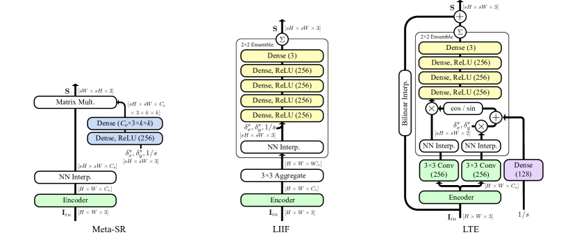
Figure 4: Previous Architectures – A visual comparison of the super-resolution architectures of Meta-SR [16], local implicit image function LIIF [6], and local texture estimators (LTE) [19], shown in an isotropic scaling configuration. Components inside the “2$\times$2 Ensemble” box are computed over the four closest pixels to compute a weighted average. The number of encoder channels, $C_{e}$, is dependent on the encoder chosen.

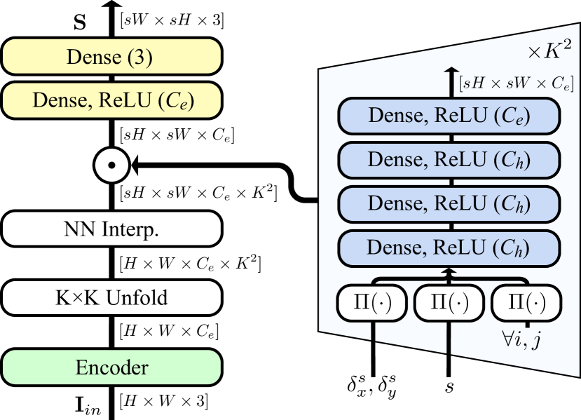
Figure 5: Architecture – Continuous Upsampling Filters (CUF) are based on a hyper-network. For each pixel position in the high-res space, the hyper-network is computed $K^{2}$ times, once for each position $i,j$ of the upsampling kernel (batched in practice). This can be reduced when upsampling with integer scales $s$, as is common in practice. The Hyper-network output is aggregated into a tensor that is dot multiplied against the unfolded nearest-neighbor interpolation, computing a depth-wise convolution with per-pixel filters. The number of encoder channels, $C_{e}$, is dependent on the encoder used. In our experiments, we set the number of hyper-network channels, $C_{h}=32$.

	Hyper Network				Upsampler
	input	#layers // #neurons	output	params (K)	input	layers	neurons	params (K)
Meta-SR [16]	$[\delta^{s}(\mathbf{x}),1/s]$	2 // 256	$64\times 9\times 3$	445	$\mathcal{E}_{\boldsymbol{\theta}}$	convolution	–	–
LIIF [6]	–	–	–	–	$[\mathcal{E}_{\boldsymbol{\theta}},\delta^{s}(\mathbf{x}),1/s]$	5 dense	256	347
LTE [19]	–	–	–	–	$h_{a}(\mathcal{E}_{\boldsymbol{\theta}})\{sin,cos\}(\delta^{s}(\mathbf{x})\pi(h_{b}(\mathcal{E}_{\boldsymbol{\theta}})+h_{c}(1/s))$	4 dense	256	494
Ours:	$[\Pi(\delta^{s}(\mathbf{x})),\Pi(s),\Pi(k)]$	4 // 32	64	6	$\mathcal{E}_{\boldsymbol{\theta}}$	d-w conv. + 2 dense	64	4

Table 1: Super-resolution with neural-fields: An overview of the main characteristics of neural field based architectures. Square brackets represent concatenation. In LTE [19], $h_{a}$,$h_{b}$ are $3\times 3$ convolutional layers and $h_{c}$ is a linear layer.

The application of neural fields to super-resolution [16] has enabled the design of architectures that support multiple target scales, as well as non-integer super-resolution scales.

• In meta super-resolution MetaSR [16], a hyper-network is conditioned on the target scale factor and on the output pixel relative coordinates (ie. the difference between source and target grids covering the same normalized global space). Their model consists of: (1) transforming the input image using an encoder into deep features at the source resolution; (2) upsampling the deep features into the target space (using nearest-neighbors); (3) using the hyper-network to produce a filter set per target relative position and scale; (4) processing the enlarged target resolution feature map into the final output using the corresponding weights.

• In local implicit image function LIIF [6], the author eliminates the use of a hyper-network (MetaSR, step 3) by extending the sampled target resolution features (step 2) with extra channels representing the relative coordinates and target scale. Their combined features are further processed through a stack of five dense layers inspired by the multi-layer perceptron (MLP) architecture typically adopted as the end-to-end model in neural-fields formulations.

• In local texture estimator LTE [19] the authors enhance the features fed as input to the MLP layers. In their model, the output of the encoder is processed by three extra trainable layers associated with the amplitude, frequency and phase of sin/cosine waves. The resulting projection in the target resolution layer is used as the input to an MLP that stacks $4$ fully-connected layers. In order to further improve the results they also adopt a global skip connection with a bilinear up-scaled version of the input around the full model, such that the deep model focus on the computation of the residual between to the closed form approximation and the final result.

A visualization of these architectures can be found in Figure 4. In practice, LIIF and LTE also increase the number of feature channels as their MLP layers have more neurons ($256$) than the number of channels produced as the encoder output ($64$ for encoders such as EDSR [21] and RDN [38]). In contrast to these previous works, our upsampler:

• Moves the computational burden of arbitrary upsampling into the continuous upsampler operator while reducing the operations performed in the target resolution space, preserving the number of channels produced by the deep encoder.

• Requires fewer operations than the single-scale sub-pixel convolution in the most typical application case of up-sampling an image by an integer scale factor, and producing results of comparable quality.

• Adopts a neural-fields formulation that focuses the sensitivity of our hyper-network to fine-grained changes in the representation of scale and relative position (reducing spectral bias).

3 Method

Given a target scale $s$, we aim to produce an upscaled image of size $sH{\times}sW{\times}3$ given an input image of size $H{\times}W{\times}3$. Within the context of super-resolution, our core contribution is the introduction of a novel learnable upsampling layer. The upsampling layer can be interpreted as a decoder in a classical encoder-decoder architecture. We briefly review our encoder architecture in Section 3.1, and detail our decoder in Section 3.2. Note that our analysis focuses on the decoder, as a variety of encoders can be used. In Section 3.4, we then perform a conceptual comparison between our architecture, shown in Figure 5, and others based on neural fields, which are visually summarized in Figure 4.

Training

Our network with parameters ${\boldsymbol{\theta}}$ is trained to regress a high resolution image $\tilde{\mathbf{I}}^{s}$ matching the ground truth $\tilde{\mathbf{I}}^{s}_{\text{gt}}$ at random positions $\mathbf{x}$ given the low resolution input image $\mathbf{I}$:

$$\operatorname*{arg\,min}_{\boldsymbol{\theta}}\>\>\mathbb{E}_{\mathbf{I}}\>\mathbb{E}_{s}\>\mathbb{E}_{\mathbf{x}}\>\|\tilde{\mathbf{I}}^{s}(\mathbf{x};\mathbf{I},{\boldsymbol{\theta}})-\tilde{\mathbf{I}}^{s}_{\text{gt}}(\mathbf{x})\|_{2}^{1}$$ (1)

3.1 Encoder

Towards this objective, we first process our input image with an encoder producing $C$-dimensional features:

$$\mathcal{E}_{\boldsymbol{\theta}}:\mathbb{R}^{H{\times}W{\times}3}\rightarrow\mathbb{R}^{H{\times}W{\times}C}$$ (2)

and then unfold a $k{\times}k$ spatial neighborhood of $C$-dimensional features into a tensor of $C{\times}k^{2}$ channels. Finally, we upsample the encoded image using nearest-neighbour interpolation. We define this step as:

$$\mathcal{U}:\mathbb{R}^{H{\times}W{\times}C}\rightarrow\mathbb{R}^{sH{\times}sW{\times}C\times k^{2}}$$ (3)

The unfolding part of this procedure leads to feature maps that will allow us to implement depth-wise, spatial convolutions as dot products, as is typically done for low-level neural network implementations. We define this whole feature extraction procedure as:

$$\mathbf{F}=\mathcal{U}(\mathcal{E}_{\boldsymbol{\theta}}(\mathbf{I}))$$ (4)

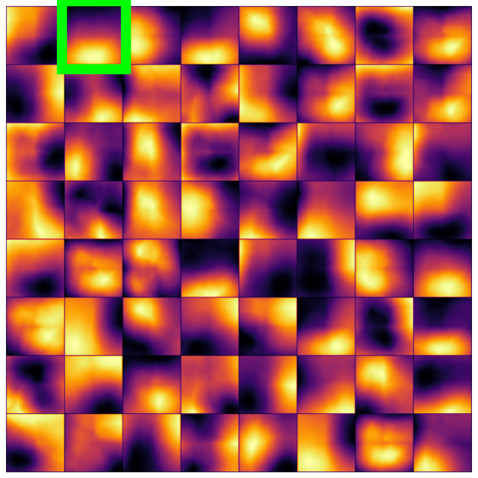
all filters

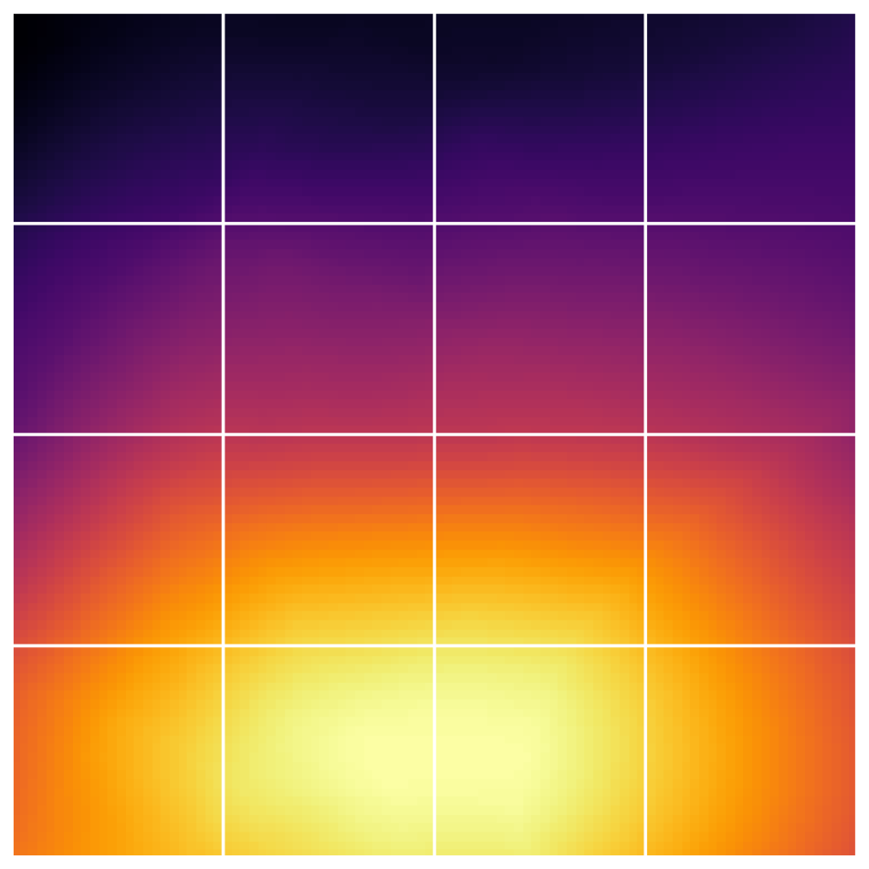
filter #2 - continuous

filter #2 - discretized

Figure 7: Continuous filters – CUF filters are continuous functions stored in neural fields. We visualize our filters by densely sampling each on the $[0,1]^{2}$ domain to highlight their continuous nature (left). Close-up of an exemplar filter (middle). Filters are discretized by sampling at pixel centers (right), allowing them to be used in classical fixed-scale super-res architectures.

3.2 Decoder – “Continuous Upsampling Filters”

We draw our inspiration from classical sub-pixel convolutions [29], and combine it with recent research that apply neural fields for continuous super-resolution [6, 19]. Differently from these architectures, we achieve this objective by instantiating upsampling kernels $\mathcal{K}$ via hyper-networks [13]. Our super-resolution network is algebraically expressed as:

$$\tilde{\mathbf{I}}^{s}(\mathbf{x};\mathbf{I},{\boldsymbol{\theta}})=\mathcal{D}_{\boldsymbol{\theta}}(\mathcal{K}_{\boldsymbol{\theta}}(\delta^{s}(\mathbf{x});s)\cdot\mathbf{F}(\lfloor\mathbf{x}/s\rfloor))$$ (5)

where $\mathbf{x}$ indexes pixel locations in the target resolution, and $\delta^{s}(\mathbf{x}){=}\bmod(\mathbf{x},s)/s$ renders our convolutional filters translation invariant, and the dot product implements a spatial convolution. The network $\mathcal{D}$ is a point-wise layer that maps (super-resolved) features back to RGB values:

$$\mathcal{D}_{\boldsymbol{\theta}}:\mathbb{R}^{C}\rightarrow\mathbb{R}^{3}$$ (6)

This is applied to a grid of coordinates of size $\mathbb{R}^{sH{\times}sW{\times}C}$ to get an image of size $\mathbb{R}^{sH{\times}sW{\times}3}$. The coordinate $\mathbf{x}$ is continuous, hence $\mathcal{K}_{\boldsymbol{\theta}}$ is a neural field parameterization of a convolutional kernel mapping (continuous) spatial offsets and (continuous) scales to convolutional weights:

$$\mathcal{K}_{\boldsymbol{\theta}}:[0,1]^{2}\times\mathbb{R}^{+}\rightarrow\mathbb{R}^{C\times K^{2}}$$ (7)

			Set5				Set14				BSD100				Urban100
Encoder	Upsampler	Self Ens.	$\times$ 2	$\times$ 3	$\times$ 4	$\times$ 6	$\times$ 2	$\times$ 3	$\times$ 4	$\times$ 6	$\times$ 2	$\times$ 3	$\times$ 4	$\times$ 6	$\times$ 2	$\times$ 3	$\times$ 4	$\times$ 6
RDN	fixed-scale [38]		38.24	34.71	32.47	-	34.01	30.57	28.81	-	32.34	29.26	27.72	-	32.89	28.80	26.61	-
	MetaSR [16]		38.22	34.63	32.38	29.04	33.98	30.54	28.78	26.51	32.33	29.26	27.71	25.90	32.92	28.82	26.55	23.99
	CUF (ours)		38.23	34.72	32.54	29.25	33.99	30.58	28.86	26.70	32.35	29.29	27.76	25.99	33.01	28.91	26.75	24.23
	fixed-scale [38]	+${}_{\text{geo}}$	38.30	34.78	32.61	-	34.10	30.67	28.92	-	32.40	29.33	27.75	-	33.09	29.00	26.82	-
	LIIF [6]	+${}_{\text{loc}}$	38.17	34.68	32.50	29.15	33.97	30.53	28.80	26.64	32.32	29.26	27.74	25.98	32.87	28.82	26.68	24.20
	LTE [19]	+${}_{\text{loc}}$	38.23	34.72	32.61	29.32	34.09	30.58	28.88	26.71	32.36	29.30	27.77	26.01	33.04	28.97	26.81	24.28
	CUF (ours)	+${}_{\text{geo}}$	38.28	34.80	32.63	29.27	34.08	30.65	28.92	26.74	32.39	29.33	27.80	26.03	33.16	29.05	26.87	24.32
SwinIR	fixed-scale [29]		38.35	34.89	32.72	-	34.14	30.77	28.94	-	32.44	29.37	27.83	-	33.40	29.29	27.07	-
	MetaSR [16]		38.26	34.77	32.47	29.09	34.14	30.66	28.85	26.58	32.39	29.31	27.75	25.94	33.29	29.12	26.76	24.16
	CUF (ours)		38.34	34.88	32.80	29.53	34.29	30.79	29.02	26.85	32.45	29.38	27.85	26.09	33.54	29.45	27.24	24.62
	fixed-scale [29]	+${}_{\text{geo}}$	38.38	34.95	32.81	-	34.24	30.83	29.02	-	32.47	29.41	27.87	-	33.51	29.42	27.21	-
	LIIF[6]	+${}_{\text{loc}}$	38.28	34.87	32.73	29.46	34.14	30.75	28.98	26.82	32.39	29.34	27.84	26.07	33.36	29.33	27.15	24.59
	LTE+lc [19]	+${}_{\text{loc}}$	38.33	34.89	32.81	29.50	34.25	30.80	29.06	26.86	32.44	29.39	27.86	26.09	33.50	29.41	27.24	24.62
	CUF (ours)+	+${}_{\text{geo}}$	38.38	34.92	32.83	29.57	34.33	30.84	29.05	26.91	32.47	29.40	27.88	26.11	33.65	29.55	27.32	24.69

Table 2: Out-of-domain evaluation – performance on datasets not seen during training. Metrics computed on the luminance channel in the YCbCr color space, following previous work. Models using self-ensemble are marked with $+_{geo}$ and models using local self-ensemble are marked with $+_{loc}$. Legend: best 2^nd best

Multi-scale up-sampling methods - DIV2k
Encoder	Upsampler	Ens.	seen scales			unseen scales
			$\times$ 2	$\times$ 3	$\times$ 4	$\times$ 6	$\times$ 12	$\times$ 18
Bicubic			31.01	28.22	26.66	24.82	22.27	21.00
EDSR-b.	Sub-pixel conv.		34.69	30.94	28.97	-	–	–
	MetaSR		34.64	30.93	28.92	26.61	23.55	22.03
	CUF (ours)		34.70	30.99	29.01	26.76	23.73	22.20
	Sub-pixel conv.	+${}_{\text{geo}}$	34.78	31.03	29.06	–	–	–
	LIIF	+${}_{\text{loc}}$	34.67	30.96	29.00	26.75	23.71	22.17
	LTE	+${}_{\text{loc}}$	34.72	31.02	29.04	26.81	23.78	22.23
	CUF (ours)	+${}_{\text{geo}}$	34.79	31.07	29.09	26.82	23.78	22.24
RDN	Sub-pixel conv.		35.01	31.22	29.20	–	–	–
	MetaSR		35.00	31.27	29.25	26.88	23.73	22.18
	CUF (ours)		35.03	31.31	29.32	27.03	23.94	22.38
	Sub-pixel conv.	+${}_{\text{geo}}$	35.10	31.33	29.31	–	–	–
	LIIF	+${}_{\text{loc}}$	34.99	31.26	29.27	26.99	23.89	22.34
	LTE	+${}_{\text{loc}}$	35.04	31.32	29.33	27.04	23.95	22.40
	CUF (ours)	+${}_{\text{geo}}$	35.11	31.39	29.39	27.09	23.99	22.42
SwinIR	Sub-pixel conv.		35.28	31.47	29.40	–	–	–
	MetaSR		35.15	31.40	29.33	26.94	23.80	22.26
	CUF (ours)		35.26	31.52	29.52	27.19	24.07	22.49
	Sub-pixel conv.	+${}_{\text{geo}}$	35.33	31.52	29.44	–	–	–
	LIIF	+${}_{\text{loc}}$	35.17	31.46	29.46	27.15	24.02	22.43
	LTE	+${}_{\text{loc}}$	35.24	31.50	29.51	27.20	24.09	22.50
	CUF (ours)	+${}_{\text{geo}}$	35.31	31.56	29.56	27.23	24.10	22.52

Table 3: In domain evaluation: tests on DIV2K’s validation subset [25] on scales seen (2$\times$ – 4$\times$) and unseen during training (6$\times$ – 30$\times$) . Metrics taken on the RGB space. Results taken using geometric self-ensemble [21] are marked with ’$+_{\text{geo}}$’ and local-ensemble [6] with ’$+_{\text{loc}}$’. Legend: best 2^nd best

Continuous kernel indexing

We can take our continuous formulation a step further by introducing a continuous parametrization of its kernel indexes $k_{i},k_{j}$ indexing our $K\times K$ convolution weight entries. Thus, the hyper-network representing the convolution field becomes:

$$\hat{\mathcal{K}}_{\boldsymbol{\theta}}:[0,1]^{2}\times\{0,\ldots,K-1\}^{2}\times\mathbb{R}^{+}\to\mathbb{R}^{C}$$ (8)

and $\mathcal{K}_{\boldsymbol{\theta}}$ can then be constructed by $9$ invocations to $\hat{\mathcal{K}}_{\boldsymbol{\theta}}$ in the case of a $K{=}3$, and $K^{2}$ invocations in the general setting. We use $K{=}3$ throughout the paper in order to facilitate a direct comparison to pre-existing baseline models.

Equation (7) and Equation (8) are both valid ways of generating spatial kernels. The first can be seen as a multi-headed hypernetwork, while the second uses input conditioning to generate the kernel values. We use the latter in our experiments, as the layers of nonlinearities provide additional expressiveness compared to the linear transformation used in the multi-headed version. A comparison between the two is presented in Appendix D.

3.3 Positional encoding

Naively representing signals with MLPs leads to “spectral bias” [26]: the overall difficulty these networks have in representing high-frequency signals. Hence we implement $\mathcal{K}_{\boldsymbol{\theta}}$ as:

$$\mathcal{K}_{\boldsymbol{\theta}}(\delta^{s}(\mathbf{x}),s,k)=\text{MLP}(\Pi(\delta^{s}(\mathbf{x})),\Pi(s),\Pi(k))$$ (9)

where we apply positional encoding $\Pi(\cdot)$ to the MLP inputs. Several variants of positional encoding exist, including Fourier [24] and random Fourier [30] variants. However, as we strive for efficiency, we take inspiration from classical signal processing (e.g. JPEG) and instead employ a cosine-only transformation. Given a scalar $f_{n}$ sampled uniformly in the range $[0,f_{\text{max}}]$, a scalar quantity $z\in[0,1]$ is encoded as the (sorted) vector:

$$\Pi(z)=\left\{cos\left(\frac{(2z+1)f_{n}\pi}{2}\right)\right\}_{n=1}^{N}$$ (10)

By eliminating the imaginary component from the Fourier basis, we show in Section 4.3 how this reduces the number of trainable parameters of the first hyper-network layer by half, without affecting super-resolution quality.

3.4 Analysis

We now perform a conceptual comparison of our network architecture to the commonly used Sub-Pixel Convolution, as well as several super-resolution approaches based on neural-fields. We further note how continuous upsampling filters can be instantiated to generate filters compatible with Sub-Pixel Convolution.

Comparison to Sub-Pixel Convolution [29]

Sub-Pixel Convolution is the most commonly used super-resolution operator, especially when efficiency is critical. This is achieved by initially employing an expansion convolution that generates a feature map with $s^{2}N_{out}$ channels, where $N_{out}$ is a hyper parameter defining the target number of channels of the Sub-Pixel Convolution operation.

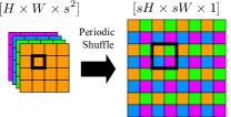
Figure 8: A simple illustration of periodic shuffling used in Sub-Pixel Convolution.

Next, the periodic shuffling operator  re-arranges the channels to produce a higher-resolution feature map (see Figure 8):

$$\mathcal{P}:\mathbb{R}^{H{\times}W{\times}C}\rightarrow\mathbb{R}^{sH{\times}sW{\times}C/s^{2}}$$ (11)

Similar to (6), whenever $N_{out}$ is chosen as different from the number of output colors, the resulting feature map is further projected by point-wise convolutions. Often, $N_{out}$ is taken as the same as the number of channels as produced by the encoder $\mathcal{E}$ for architectures adopting Sub-Pixel Convolution and targeting high quality results [21, 38, 20]. We note that the Sub-Pixel Convolution design based on the expansion convolution does not enforce spatial correlations between neighboring pixels (here we refer to neighborhood in the output, high resolution, domain) and need to be learned from training data. Conversely, these correlations are inherently captured by our continuous convolutional filters.

Further, in the integer scale setup where hyper-networks can be pre-instantiated, CUFs are computationally more efficient than sub-pixel convolutions whenever $K^{2}+N_{in}+N_{out}<N_{out}\times K^{2}$ (in the worst case scenario) as the cost associated with pre-computing the weights for a given integer up-sampling scale can be neglected when compared to the operations performed on the image grid (see Appendix E).

Comparisons to LIIF [6] and LTE [19]

In comparison to these works, we make the main network shallower ($1$ depth-wise continuous convolution and $2$ dense layers) in order to reduce the number of layers that operate at the target spatial resolution and at the encoder’s channel resolution. At the same time, our upsampler head is considerably lighter than previous arbitrary scale methods, not only by the use of a depth-wise convolution but also by keeping the same number of channels produced by the features encoder in the main network ($C_{e}=64$, which results in dense layers $16\times$ cheaper than its LIIF and LTE counterparts using $256$ neurons). When performing non-integer upsampling, the costs with processing the hyper-network layers are proportional to the target image resolution, but still smaller than a single dense layer of LIFF and LTE heads, due to the adoption of a reduced number of channels (as $C_{h}=32$, each of CUF’s hypernetwork dense layers is $64\times$ cheaper than LIIF and LTE layers using $256$ neurons).

Instantiating CUFs

At inference time, when targeting an integer upscaling factor $s$, the hyper-network representing $\mathcal{K}$ can be queried to retrieve the weights corresponding to $s^{2}$ relative subpixel positions as an initialization step during pre-processing. The retrieved weights are re-used across all pixels taking advantage of the existent periodicity. Thus, in the CUF-instantiated architecture the continuous kernel is replaced at test time with a discrete depth-wise convolution, followed by a pixel shuffling operation, in contrast with the unfolding operator used in the regular, fully continuous CUF described in this paper. Otherwise, the architecture remains the same. The costs associated with the hyper network at initialization can be neglected as $s^{2}<<sH\times sW$. In this setting, our model becomes as efficient as a sub-pixel-convolution architecture, while retaining the aforementioned continuous modeling properties at training time.

4 Results

In this section we describe our experimental setup in terms of backbone encoders and training/validation dataset, perform careful comparisons to the state-of-the-art (Section 4.1), and additional evaluation towards the implementation of lightweight super-res architectures (Section 4.2). We conclude by performing a thorough ablation (Section 4.3).

Method	Composition	Parameters (in M)
		encoder	spc. $4\times$
RDN	Convolutions	22.00	0.30
SwinT	Conv. and Self-Attention	11.60	0.30
EDSR-baseline	Convolutions	1.20	0.30
SwinT-lightweight	Conv. and Self-Attention	0.90	0.03
ABPN	Convolutions	0.03	0.03

Table 4: Encoders – Our experiments use CUF layers in combination with various encoders differing in composition and size. Parameter counts reflect the encoder size and the upsampling head using a Sub-Pixel Convolution (spc) targeting $4\times$ upsampling.

Urban100 - #008

LR

GT

SwinIR + LIIF $\times$ 4

SwinIR + LTE $\times$ 4

SwinIR + CUF $\times$ 4

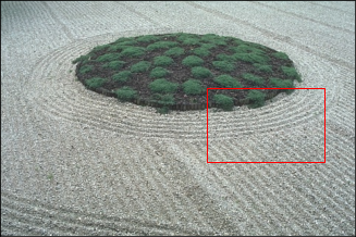
B100 - #86016

LR

GT

EDSR + LIIF $\times$ 3

EDSR + LTE $\times$ 3

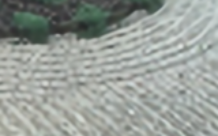
EDSR + CUF $\times$ 3

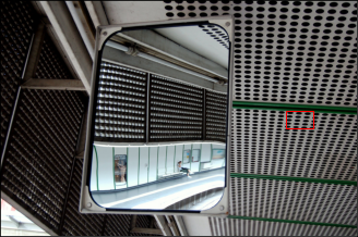
Urban100 - #030

LR

GT

EDSR + LIIF $\times$ 4

EDSR + LTE $\times$ 4

EDSR + CUF $\times$ 4

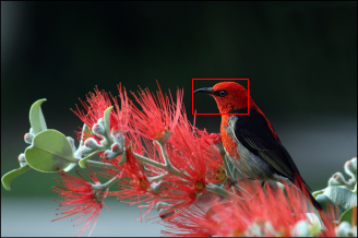
Urban100 - #008

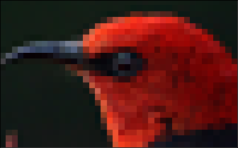
LR

GT

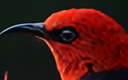
RDN + LIIF $\times$ 8

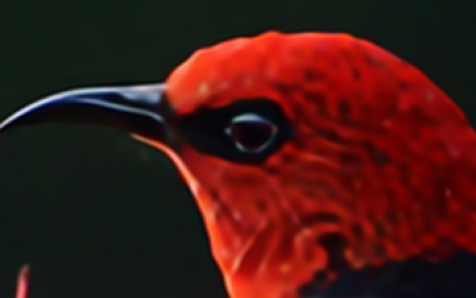
RDN + LTE $\times$ 8

RDN + CUF $\times$ 8

Figure 11: Qualitative evaluation – CUF combined with different encoders and upsampling scales.

Encoders

We apply CUFs to a variety of encoders, to both show its generality, as well as its performance gains in a variety of settings.

• A state-of-the-art encoder for super-res named SwinIR [20] based on Swin-transformers [22].

• Well-known convolution-based encoders, namely EDSR-baseline [21] and Residual Dense Networks (RDN) [38].

• Architectures for lightweight and extremely lightweight inference, respectively SwinT-lightweight [20] and ABPN [10].

Table 4 contrasts the ablated encoders’ composition and size. Hyperparameter settings can be found in the appendix.

Datasets

All models are trained using the DIV2K dataset training subset ($800$k images), introduced at the NTIRE 2017 Super Resolution Challenge [25]. Similarly to previous works, each image is randomly cropped 20 times per epoch and augmented with random flips, and 90 degrees rotations. We report peak signal-to-noise ratio (PSNR) results on the DIV2K validation set (100 images), in the RGB space. To understand the generalizability of our experimental results, we test our models on additional well known datasets (Set5 [4] – 5 images; Set14 [36] – 14 images; B100 [23] – 100 images; and Urban100 [17] – 100 images), in which, following previous works, PSNR is measured in the YCbCr luminance channel.

Ensembling

Whenever demarked by ‘$+_{\text{geo}}$’, results incorporate the (commonly adopted) Geometric Self-ensemble [21], where the results of rotated versions of the input images are averaged at test time. LIIF and LTE results adopt Local Self-ensemble (‘$+_{\text{loc}}$’), where the result of applying the upsampler at $4$ shifted grid points is averaged, resulting in a $\times 4$ increase in computational complexity at training/test time. It may also introduce confounding factors to the optimization process that invalidate direct comparison to the fixed-scale upsamplers, as during back-propagation the encoder gradients are averaged. In Appendix B we combine these models.

4.1 State-of-the-art comparisons

Table 2 and Table 3 show the quantitative comparisons, while qualitative results can be observed in Figure 3, Figure 11 and Appendix F. Table 3 contains in-domain results: models trained on DIV2k and tested on DIV2k (train/test split), while Table 2 presents out-of-domain results: models are trained on DIV2k, but tested on different datasets.  Note that upsampling ratios larger than $\times 4$ are not provided at training time. The models adopting sub-pixel convolutions are fixed-scale models, that is, one model is trained per target scale and thus do not generalize to unseen or fractional scales. On the remaining rows we present results of arbitrary-scale upsamplers (MetaSR [16], LIIF [6], LTE [19]), where a single model is trained and tested across different upsampling ratios.  Our method is the first arbitrary-scale method to match (or surpass) fixed-scale performance across all encoders in both single-pass inference and self-ensemble scenarios.

Multi scale up-sampling methods
		Set5				Set14				BSD100				Urban100
Encoder	Upsampler	$\times$ 2	$\times$ 3	$\times$ 4	$\times$ 6	$\times$ 2	$\times$ 3	$\times$ 4	$\times$ 6	$\times$ 2	$\times$ 3	$\times$ 4	$\times$ 6	$\times$ 2	$\times$ 3	$\times$ 4	$\times$ 6
SwintIR-light [20]	Sub-Pixel Conv.	38.14	34.62	32.44	–	33.86	30.54	28.77	–	32.31	29.20	27.69	–	32.76	28.66	26.47	–
	CUF (ours)	38.17	34.62	32.46	29.09	33.93	30.57	28.83	26.61	32.30	29.23	27.71	25.95	32.73	28.68	26.55	24.11
ABPN[10]	Sub-Pixel Conv.	37.30	33.39	31.11	–	32.90	29.68	27.97	–	31.67	28.64	27.14	–	30.37	26.77	24.96	–
	CUF (ours)	37.35	33.55	31.31	28.06	32.96	29.74	28.04	25.86	31.72	28.69	27.19	25.52	30.53	26.92	25.05	23.01

Table 5: Lightweight super-res – Our CUFs enable continuous super-resolution with lightweight (SwinIR-lightweight [20]) and mobile-friendly (ABPN [10]) backbones without quality loss.

4.2 Lightweight super-resolution

The encoders and upsamplers considered so far are not designed to be run on devices with limited memory and power. Running super-resolution algorithms on mobile devices comes with unique challenges due to limited RAM and non-efficient support for certain common operations [18]. The proposed CUF-based upsampler, in combination with a mobile-compatible encoder, can be effectively used for upscaling on mobile devices.

To test the effectiveness of the CUFs, we adopt a lightweight version of SwinIR ($0.9$M parameters) [20] as well as one of the best performing super-lightweight architectures for mobile devices ($30$K parameters) [10] as the encoder. For the latter, the original architecture (Figure 12, left) consists of a lightweight encoder and an upscaling module consisting of a series of convolutions, ReLU’s, and a standard periodic shuffle layer. We replace this upscaling module with a CUF-based one (Figure 12, right). With instantiated CUFs, this means simply introducing a depthwise convolution followed by pointwise layers, where the weights are output by the learned CUFs.

Table 5 illustrates that CUFs provide the same level of accuracy while enabling continuous scale and efficient inference. To our knowledge, this is the first mobile-friendly continuous scale super-resolution architecture.

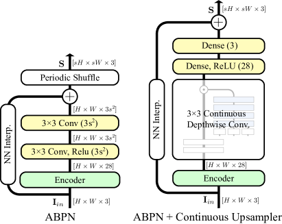
Figure 12: Architectures (lightweight) – The original ABPN [11] single scale architecture (left) and our arbitrary-scale version using the implicit upsampler (right). Note how the two consecutive $3\times 3$ native convolutions are exchanged for a $3\times 3$ depth-wise implicit convolution followed by point-wise layers.

4.3 Ablations

We run several ablation experiments in order to analyze the effects of various model choices. Here, we detail our choice of using DCT for positional encoding vs Fourier features, as well as an investigation of the redundancy of CUF filters versus subpixel convolution. An analysis on the various conditioning factors of our neural fields (positional encoding, kernel indices, scale, and target subpixel) can be found in the appendix.

Positional encoding

A large body of work uses a Fourier basis for the positional encodings, e.g. [24, 31]. However, we opt to use a DCT basis as this requires half of the sinusoidal projections and neurons at the hyper-network first layer. This trick has been used in other domains, such as random approximations of stationary kernel functions [27].

	$2\times$	$3\times$	$4\times$
Fourier	30.45	26.85	25.00
DCT	30.44	26.86	25.00

Table 6: Cosine basis – matching results but using half of sinusoidal projections and neurons at the hyper-network input. PSNR from Urban-100 dataset using a ABPN encoder.

In Table 6 we show the PSNR, as obtained using a DFT versus a DCT basis, and verify that we do not observe loss in performance, while at the same time saving half of the computation associated with positional encoding operations.

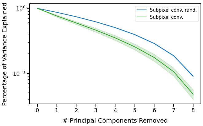
(a) Subpixel Convolutions

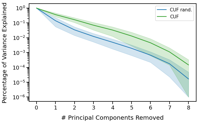
(b) CUF

Figure 13: CUF depthwise continuous filters are low rank by construction. Subpixel-convolution fails to find low rank filters.

Redundancy of filters

As noted in Section 3.4, sub-pixel convolution does not enforce spatial correlation between neighboring weights in its convolutional filters, but has to learn them from data. CUF on the other hand generates the filters with a hypernetwork, which intrinsically builds on smoothness due to its functional form. Here, we test this hypothesis on the filters of CUF and sub-pixel convolutions. For this analysis, we use an EDSR encoder with $C_{e}=64$, $K=3\times 3$, and $s=3$. Subpixel convolution maps $C_{e}$ features to $s^{2}C_{e}$ features, and each group of $s^{2}$ output features are rearranged to form the upscaled feature space. We therefore consider each group of $s^{2}$ filters of size $K\times K\times C_{e}$ and do an eigenvalue analysis to determine the compressibility of these filters. This is done by forming $C_{e}$ separate matrices of size $s^{2}\times C_{e}K^{2}$ and performing PCA on each of them separately, forming $64$ separate sets of eigenvalues. We plot this distribution for trained and untrained sub-pixel layers in Figure 13(a). A faster decay means more redundancy, as more variance is explained by fewer components. In this case, training adds significant structure to the filters.

Conversely, each output channel in CUF is computed by $s^{2}$ filters of size $K\times K$. These are not directly comparable to subpixel convolution, but we perform an analogous eigenvalue analysis on trained and untrained CUFs. As shown in Figure 13(b), unlike subpixel convolution, CUFs actually become less redundant with training, suggesting that the initial hypernetwork already imposes a very smooth prior on the filters. In other words, CUF filters incorporate spatial correlations from the very beginning due to their functional form.

5 Conclusions

We propose CUF, a computationally efficient modeling of continuous upsampling filters as neural fields. Different from previous arbitrary-scale architectures, the performance gains obtained by our upsampler are not due to increased capacity but rather to a more efficient use of model parameters. A single hyper-network supports filter adaptation across scales while at the same time CUF’s upsampling head has fewer parameters than previous arbitrary-scale heads, as well as fewer parameters than a single Sub-Pixel Convolution head at $4\times$ upsampling. CUF is the first arbitrary scale model that can be effectively used for upscaling on mobile devices, an area previously dominated by single scale Sub-Pixel Convolution architectures.  CUF’s archtecture is quite general. A natural direction of future work is to investigate its use for architectures with multiple upsampling layers (and the reuse of filters across scales) and for different image generation settings such as GANs [12] and diffusion models [15].  Neural fields have done particularly well on higher-dimensional signals. Another line of future work is the use of CUF for efficient super-resolution of video data.

CUF: Continuous Upsampling Filters
Supplementary Material

Appendix A Experiment details

Training Hyper-parameters

Encoder	Batch	Crop	Initial LR
EDSR-baseline [21]	16	48	$1e^{-4}$
RDN [38]	16	48	$1e^{-4}$
SWINIR [20]	32	48	$2e^{-4}$
SWINIR-lightweight [20]	64	64	$2e^{-4}$
ABPN [10]	16	64	$1e^{-3}$

Table 7: Training hyper-parameters: replicate each encoder’s original setting.

Table 7 contains the hyper-parameters used for training the ablated models, taken from their single-scale (Sub-Pixel Conv.) training settings. All models are trained for $1K$ epochs with $\mathcal{L}_{1}$ loss and ADAM optimizer by setting $\beta_{1}=0.9$, $\beta_{2}=0.999$, and $\epsilon=1e^{-8}$. We use a step-wise learning rate schedule that is halved at epochs $[500,800,900,950]$. Unless referred as single-scale, models were trained with random scales by sampling the scale factor uniformly within the continuous interval $[1,4]$. In order to ensure that the dimensions within the training mini-batch match despite heterogeneous scale factors, we first scale each image as required and then apply the same crop size to both LR and HR images, such that the HR random crop contains $1/s^{2}$ of the content of the LR crop, and fix the relative grid coordinates to point to the random subregion.

Encoder	$C_{e}$	$C_{h}$	Params(K)
EDSR-baseline	64	32	10
RDN
SWINIR
SWINIR-lightweight	60	32	10
ABPN (k as input)	28	28	5
ABPN (k as output)			11

Table 8: CUF’s hyper-parameters: $C_{e}$ chosen as each the encoder output features.

CUF’s hyper parameters

Table 8 describes the number of neurons used in the presented ablations across different encoders. $C_{e}$ was chosen to replicate the original number of output features of each encoder. CUF’s hyper-parameters were obtained by grid search on the EDSR-baseline and Set5 dataset and replicated on the remaining encoders. CUF’s positional encoding hyper-parameters enforce a small number of basis per input parameter. For each input (represented in $2D$ space), the number of basis $N^{2}$ was searched within the set $\{0,1^{2},2^{2},...,5^{2}\}$ while $f_{\text{max}}$ within the set $\{0,0.5,...,4.0\}$ for $\Pi(\delta^{s}(\mathbf{x}))$ and $\Pi(s)$, and within the set $\{0,0.5,..,3.0\}$ for $\Pi(k)$. The final positional encoding hyper-parameters adopted are $\Pi(\delta^{s}(\mathbf{x});):\{N^{2}=25;f_{\text{max}}=2.0\}$, $\Pi(s):\{N^{2}=25;f_{\text{max}}=2.0\}$ and $\Pi(k):\{N^{2}=9;f_{\text{max}}=1.0\}$.

Appendix B On the use of ensemble

Multi-scale up-sampling methods - DIV2k
Encoder	Upsampler	Ens.	seen scales			unseen scales
			$\times$ 2	$\times$ 3	$\times$ 4	$\times$ 6	$\times$ 12
EDSR-baseline [21]	Sub-pixel conv.		34.69	30.94	28.97	–	–
	LIIF		34.63	30.95	28.97	26.72	23.66
	LTE		34.63	30.99	29.01	26.77	23.74
	CUF (ours)		34.70	30.99	29.01	26.76	23.73
	Sub-pixel conv.	+${}_{\text{geo}}$	34.78	31.03	29.06	–	–
	LIIF	+${}_{\text{geo}}$	34.74	31.05	29.07	26.80	23.76
	LTE	+${}_{\text{geo}}$	34.72	31.07	29.08	26.83	23.79
	CUF (ours)	+${}_{\text{geo}}$	34.79	31.07	29.09	26.82	23.78

Table 9: Disentangling the effect of ensembling on optimization: Models trained under same supervision (no ensemble), and tested with (marked with $+_{geo}$) and without geometric self-ensemble. Results on DIV2K’s validation subset [25].

The baseline settings from LIIF [6] and LTE [19] include locally ensembling pixels around the target sub-pixel, by shifting by its position by half pixel in the low resolution grid, and averaging their results. This procedure introduces a training and inference overhead, as the sampled points is increased by a factor of four. As a direct consequence, during training models adopting local self-ensemble evaluate four times more gradients per optimization step. In order to disentangle possible optimization side effects, in this section we ablate the models LIIF and LTE under same optimization conditions as other models, that is, no ensemble is adopted during training, but on inference time only. LTE presents a strong result on scales $3$ and larger, but a reduction in performance on scale $2$, in which LIIF matches or surpass its performance. Overall, this ablation confirms the benefits from CUF as the lighter arbitrary scale upsampler with strong performance under single pass and self-ensemble settings, across both smaller and larger scales.

Appendix C On the use of positional encoding

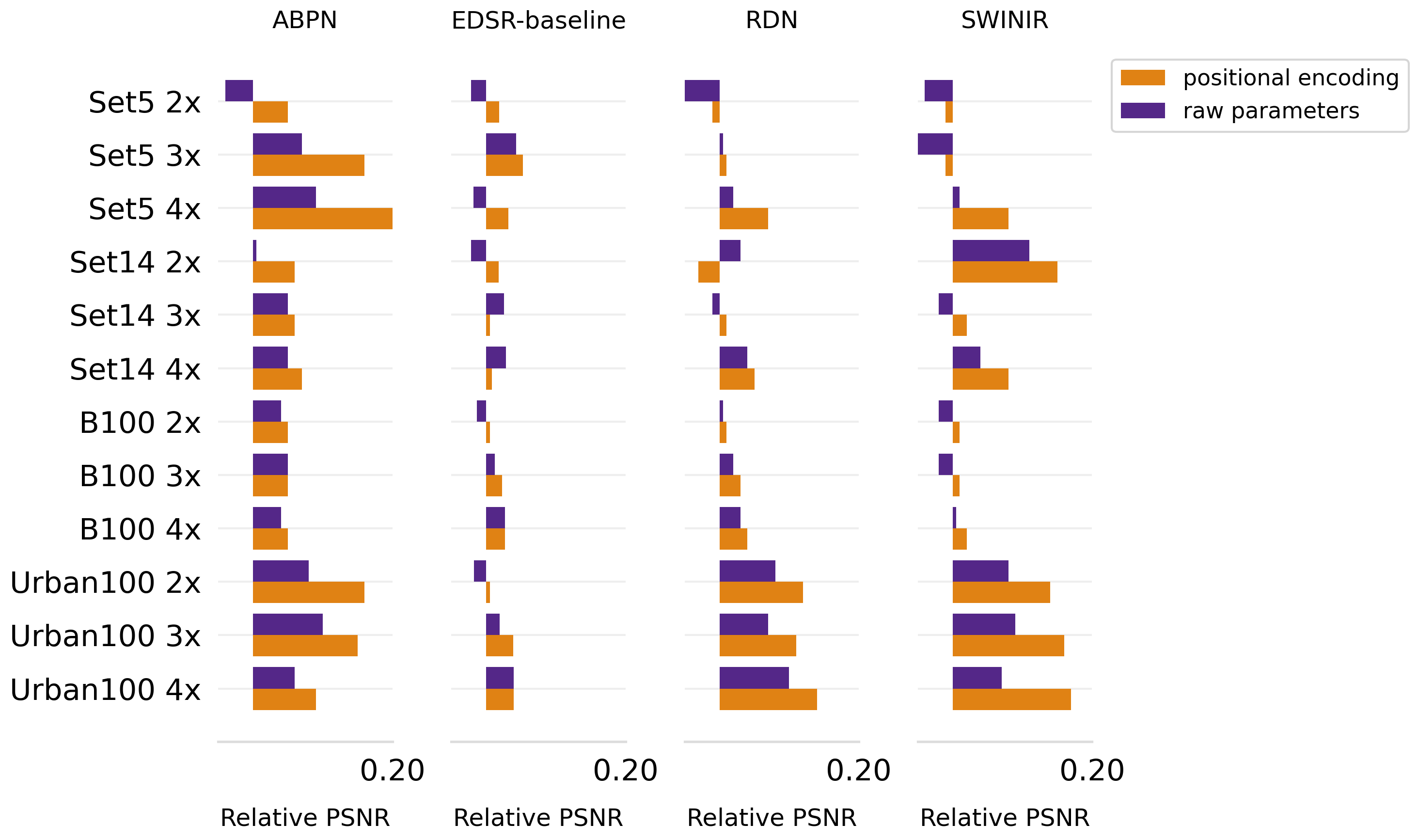
Figure 14: Impact of CUF’s positional encoding on different datasets and encoders. Bar plots represent PSNR differences relative to baseline models adopting sub-pixel convolutions and corresponding encoder.

HR

LR

LR crop

w/o. pos. enc.

with. pos. enc.

GT ($\times$ 3)

LR crop

w/o. pos enc

with. pos enc

GT ($\times$ 3)

Figure 17: Qualitative evaluation on mobile-compatible encoder – ABPN-CUF with and without positional encoding. Butterfly image from Set5 dataset.

Figure 14 contains a comparison of CUF models trained using the neural-fields parameters as raw values versus the projection using positional encoding. The stronger impact of using positional encoding is observed on ABPN encoder (Figure 17) and Urban-100 dataset [17]. We note that the content of this dataset is characterized by sharp straight lines and geometric structures, thus the quantitative gain is aligned with the expected behaviour.

Appendix D Conditioning on the kernel indexes

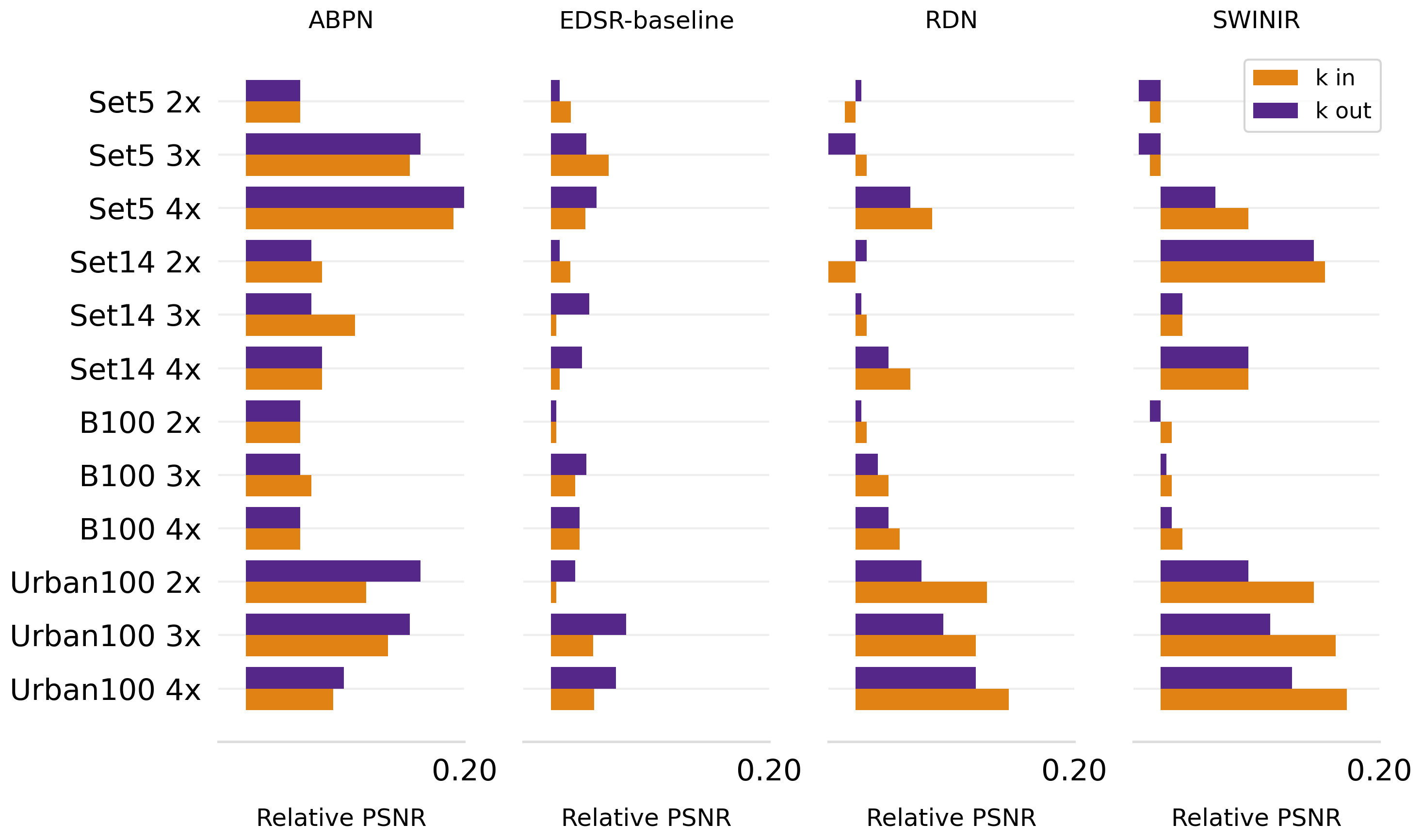
Figure 18: Comparison between conditioning the neural-fields on the kernel indexes $(k_{i},k_{j})$ versus its discretization at the hyper-network output layer. Stronger encoders take advantage of the hyper-network depth and non linearities. Bar plots represent PSNR differences relative to baseline models adopting sub-pixel convolutions and corresponding encoder.

Figure 18 contains a comparison between representing the kernel indexes $k_{i},k_{j}$ as input parameters to the neural-fields versus representing their discrete set as individual neurons at the output of the hyper-network. On the efficiency side, setting them as the hyper-network output neurons reduces memory and computation used, as hidden layers are shared. On the other hand, the layers of the hyper-network and its nonlinearities provide additional expressiveness compared to the linear transformation used in the multi-headed version. This additional expressiveness results in in performance improvement in stronger encoders (RDN, SWINIR), but not on smaller ones (ABPN, EDSR). Thus, we recommend conditioning on kernel indexes only for those encoders that take advantage of it.

Appendix E Sub-Pixel Convolution vs. CUF-instantiated

In this section we compare the costs associated with Sub-Pixel Convolution and CUF-instantiated upsampling heads. The presented comparison contrasts their designs choices based on full convolution (Sub-Pixel Convolution) versus depthwise-pointwise decomposition (CUF). As unitary element of comparison we evaluate the number of multiplications performed to produce a single output pixel. We assume an input feature map with $C_{in}$ channels, the resulting image with $C_{out}$ channels and that both Sub-Pixel Convolution and CUF-instantiated adopt filters of same size $K$.

CUF-instantiated architecture is composed with a depthwise convolution and pointwise projections. Its three layers perform respectively $C_{in}*k^{2}$, $C_{in}*C_{in}$ and $C_{in}*C_{out}$ multiplications per output pixel.

Next, we cover two common compositions with Sub-Pixel Convolution. The most common design for upsampler heads targeting high quality results is to combine a Sub-Pixel Convolution layer with a pointwise layer projecting from $C_{in}$ into RGB channels ($C_{out}$) ([21, 38, 20]). In this setting, both Sub-Pixel Conv. and CUF-instantiated have identical output layers, that is removed from our analysis. The number of multiplications performed by the Sub-Pixel Convolution layer alone per target subpixel is: $C_{in}*k*k*C_{in}$. Thus, the fraction of multiplications performed by CUF-instantiated in relation to Sub-Pixel Convolution can be expressed as: $\frac{k^{2}+C_{in}}{k^{2}*C_{in}}=\frac{1}{C_{in}}+\frac{1}{k^{2}}$. That is, the decomposition has the desired effect of saving computation whenever $C_{in},k>1$.

An alternative use of a Sub-Pixel Convolution layer is its direct use as output layer. In this case, the three layers that compose CUF’s upsampling head are compared to the full expansion convolution alone. Thus, the total operations performed by CUF-instantiated is smaller that those performed by Sub-Pixel Convolution whenever $k^{2}+C_{in}+C_{out}<k^{2}*C_{out}$.

In practice, the depthwise-pointwise decomposition adopted by CUF-instantiated faces a memory drawback of storing an extra feature map created in-between the decomposition layers $C_{in}$ (Figure 1). The reduction of such drawback with fused-convolutions is left as future work [1].

Appendix F Qualitative comparisons

The difference between existent arbitrary-scale up-samplers can only be observed at textured regions of the image. In this section we disentangle the rule of the encoder and upsampler in the perceived quality of the results. Figure 26 contain additional results, with non-integer scale factors.

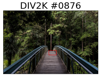
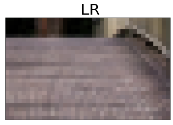
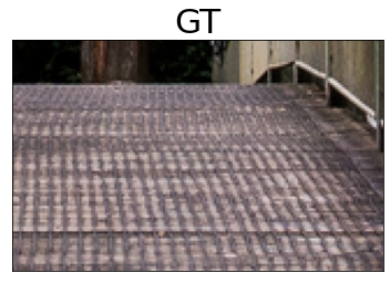
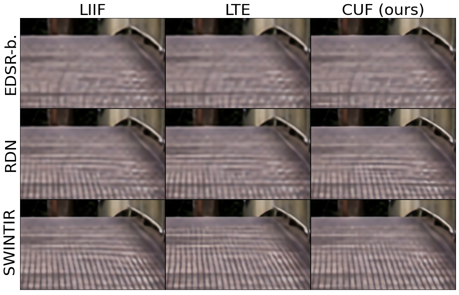
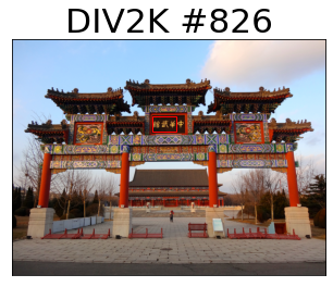
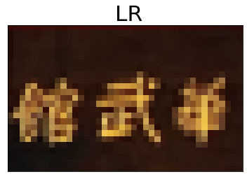
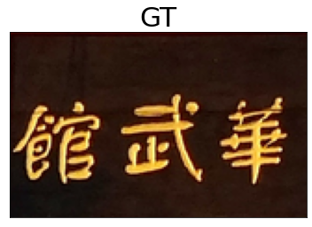
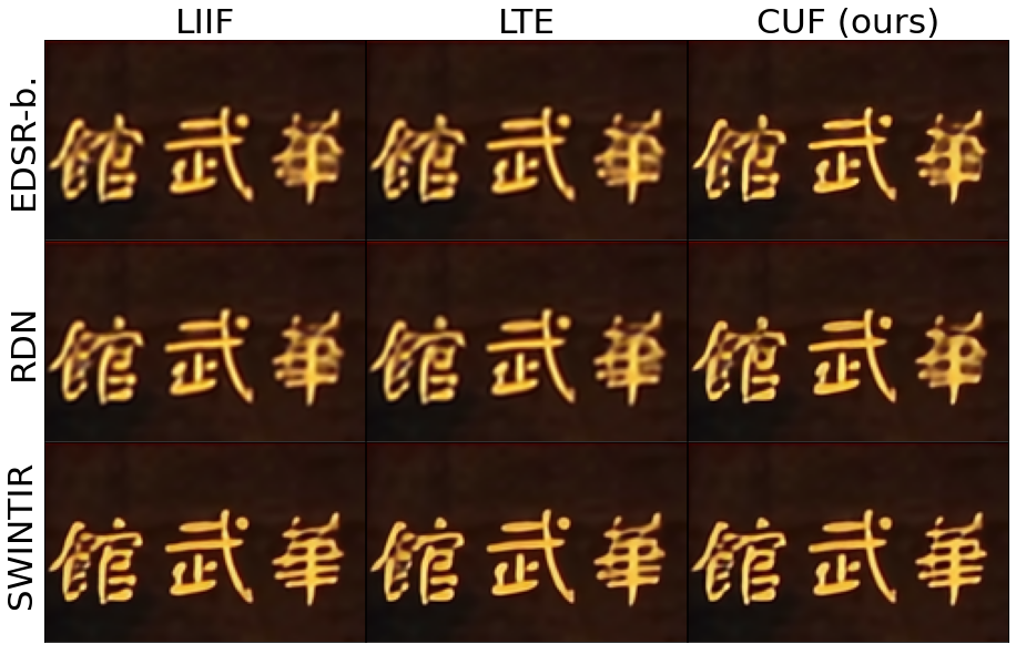
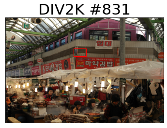
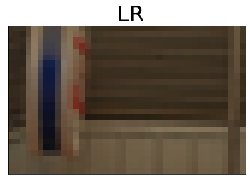
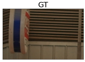
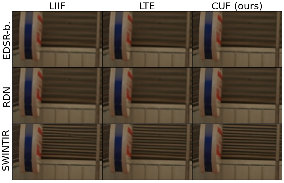
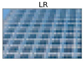
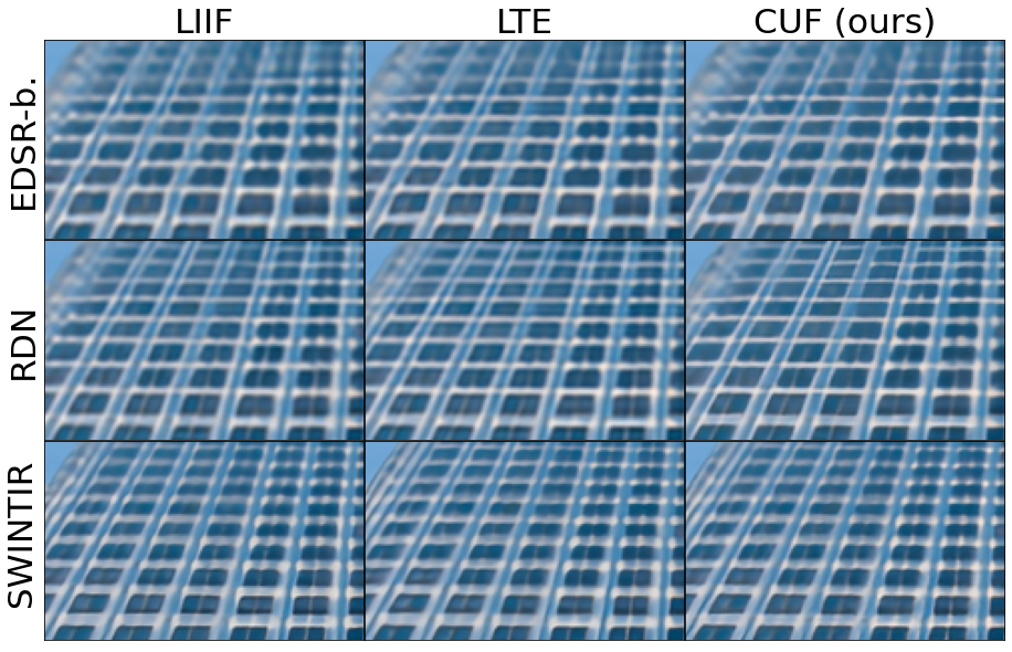
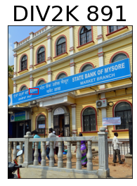
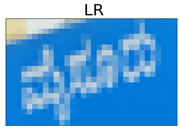
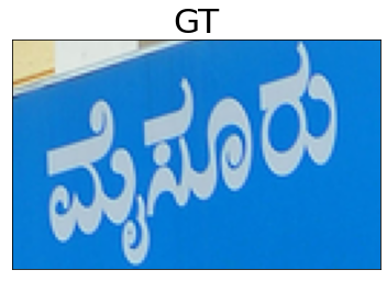
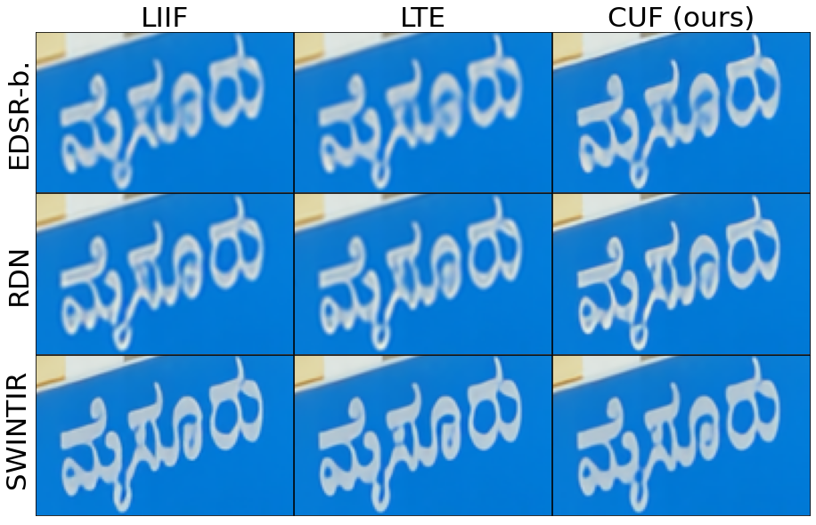
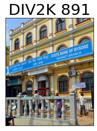
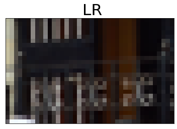
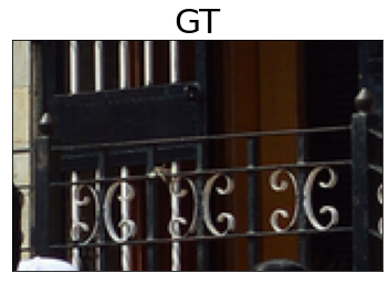
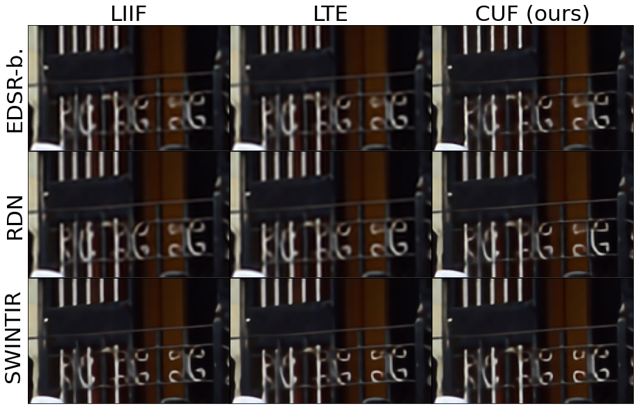
Figure 21: Qualitative comparisons of arbitrary-scale super resolution methods using different encoders. Scale factor $4\times$

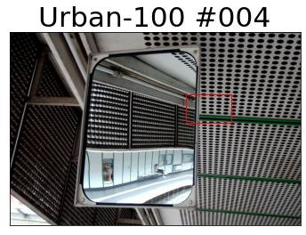
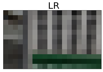
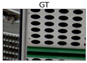
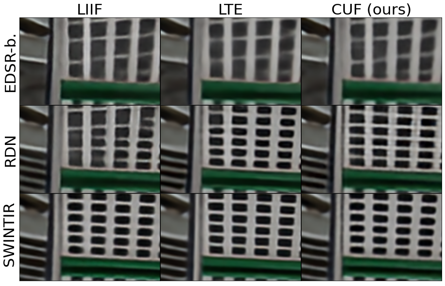
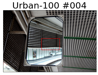
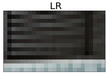
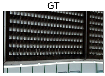
Figure 24: Hard cases: Aliasing artifacts observed on hard cases. Our upsampler produces the sharper results. Scale factor $8\times$

LR

$\times$1.5

$\times$2

$\times$2.5

$\times$3

$\times$3.5

$\times$4

$\times$4.5

$\times$5

LR

$\times$1.5

$\times$2

$\times$2.5

$\times$3

$\times$3.5

$\times$4

$\times$4.5

$\times$5

LR

$\times$1.5

$\times$2

$\times$2.5

$\times$3

$\times$3.5

$\times$4

$\times$4.5

$\times$5

Figure 26: Qualitative results using non-integer scales. Images from Set14 dataset.

References

- [1] Manoj Alwani, Han Chen, Michael Ferdman, and Peter Milder. Fused-layer cnn accelerators. pages 1–12, 10 2016.
- [2] Saeed Anwar, Salman Khan, and Nick Barnes. A deep journey into super-resolution: A survey. ACM Computing Surveys (ACMCSUR), 53(3), May 2020.
- [3] Syed Muhammad Arsalan Bashir, Yi Wang, Mahrukh Khan, and Yilong Niu. A comprehensive review of deep learning-based single image super-resolution. PeerJ Computer Science, 7:e621, Jul 2021.
- [4] Marco Bevilacqua, Aline Roumy, Christine Guillemot, and Marie line Alberi Morel. Low-complexity single-image super-resolution based on nonnegative neighbor embedding. In Proceedings of the British Machine Vision Conference, pages 135.1–135.10. BMVA Press, 2012.
- [5] Alexandre Boulch. Convpoint: Continuous convolutions for point cloud processing. Computers & Graphics, 88:24–34, 2020.
- [6] Yinbo Chen, Sifei Liu, and Xiaolong Wang. Learning continuous image representation with local implicit image function. In Proceedings of the IEEE/CVF Conference on Computer Vision and Pattern Recognition, pages 8628–8638, 2021.
- [7] Tao Dai, Jianrui Cai, Yongbing Zhang, Shu-Tao Xia, and Lei Zhang. Second-order attention network for single image super-resolution. In 2019 IEEE/CVF Conference on Computer Vision and Pattern Recognition (CVPR), pages 11057–11066, 2019.
- [8] Chao Dong, Chen Change Loy, Kaiming He, and Xiaoou Tang. Learning a deep convolutional network for image super-resolution. In David Fleet, Tomas Pajdla, Bernt Schiele, and Tinne Tuytelaars, editors, Computer Vision – ECCV 2014, pages 184–199, Cham, 2014. Springer International Publishing.
- [9] Chao Dong, Chen Change Loy, Kaiming He, and Xiaoou Tang. Image super-resolution using deep convolutional networks. IEEE Trans. Pattern Anal. Mach. Intell., 38(2):295–307, feb 2016.
- [10] Zongcai Du, Jie Liu, Jie Tang, and Gangshan Wu. Anchor-based plain net for mobile image super-resolution. In Proceedings of the IEEE/CVF Conference on Computer Vision and Pattern Recognition (CVPR) Workshops, pages 2494–2502, June 2021.
- [11] Z. Du, J. Liu, J. Tang, and G. Wu. Anchor-based plain net for mobile image super-resolution. In 2021 IEEE/CVF Conference on Computer Vision and Pattern Recognition Workshops (CVPRW), pages 2494–2502, Los Alamitos, CA, USA, jun 2021. IEEE Computer Society.
- [12] Ian Goodfellow, Jean Pouget-Abadie, Mehdi Mirza, Bing Xu, David Warde-Farley, Sherjil Ozair, Aaron Courville, and Yoshua Bengio. Generative adversarial networks. Communications of the ACM, 63(11):139–144, 2020.
- [13] David Ha, Andrew Dai, and Quoc V Le. Hypernetworks. arXiv preprint arXiv:1609.09106, 2016.
- [14] Pedro Hermosilla, Tobias Ritschel, Pere-Pau Vázquez, Àlvar Vinacua, and Timo Ropinski. Monte carlo convolution for learning on non-uniformly sampled point clouds. ACM Trans. Graph., 37(6), dec 2018.
- [15] Jonathan Ho, Ajay Jain, and Pieter Abbeel. Denoising diffusion probabilistic models. Advances in Neural Information Processing Systems, 33:6840–6851, 2020.
- [16] Xuecai Hu, Haoyuan Mu, Xiangyu Zhang, Zilei Wang, Tieniu Tan, and Jian Sun. Meta-sr: A magnification-arbitrary network for super-resolution. In Proceedings of the IEEE/CVF Conference on Computer Vision and Pattern Recognition (CVPR), June 2019.
- [17] Jia-Bin Huang, Abhishek Singh, and Narendra Ahuja. Single image super-resolution from transformed self-exemplars. In Proceedings of the IEEE Conference on Computer Vision and Pattern Recognition, pages 5197–5206, 2015.
- [18] A. Ignatov, R. Timofte, M. Denna, A. Younes, A. Lek, M. Ayazoglu, J. Liu, Z. Du, J. Guo, X. Zhou, H. Jia, Y. Yan, Z. Zhang, Y. Chen, Y. Peng, Y. Lin, X. Zhang, H. Zeng, K. Zeng, P. Li, Z. Liu, S. Xue, and S. Wang. Real-time quantized image super-resolution on mobile npus, mobile ai 2021 challenge: Report. In 2021 IEEE/CVF Conference on Computer Vision and Pattern Recognition Workshops (CVPRW), pages 2525–2534, Los Alamitos, CA, USA, jun 2021. IEEE Computer Society.
- [19] Kyong Hwan Jin Jaewon Lee. Local texture estimator for implicit representation function. Proceedings of the IEEE/CVF Conference on Computer Vision and Pattern Recognition, 2022.
- [20] Jingyun Liang, Jiezhang Cao, Guolei Sun, Kai Zhang, Luc Van Gool, and Radu Timofte. Swinir: Image restoration using swin transformer. In IEEE International Conference on Computer Vision Workshops, 2021.
- [21] Bee Lim, Sanghyun Son, Heewon Kim, Seungjun Nah, and Kyoung Mu Lee. Enhanced deep residual networks for single image super-resolution. In The IEEE Conference on Computer Vision and Pattern Recognition (CVPR) Workshops, July 2017.
- [22] Ze Liu, Yutong Lin, Yue Cao, Han Hu, Yixuan Wei, Zheng Zhang, Stephen Lin, and Baining Guo. Swin transformer: Hierarchical vision transformer using shifted windows. In Proceedings of the IEEE/CVF International Conference on Computer Vision (ICCV), 2021.
- [23] D. Martin, C. Fowlkes, D. Tal, and J. Malik. A database of human segmented natural images and its application to evaluating segmentation algorithms and measuring ecological statistics. In Computer Vision, 2001. ICCV 2001. Proceedings. Eighth IEEE International Conference on, volume 2, pages 416–423, 2001.
- [24] Ben Mildenhall, Pratul P. Srinivasan, Matthew Tancik, Jonathan T. Barron, Ravi Ramamoorthi, and Ren Ng. Nerf: Representing scenes as neural radiance fields for view synthesis. In ECCV, 2020.
- [25] et al. Radu Timofte. Ntire 2017 challenge on single image super-resolution: Methods and results. In Proceedings of the IEEE Conference on Computer Vision and Pattern Recognition Workshops, CVPRW 2017, pages 1110–1121, 2017.
- [26] Nasim Rahaman, Aristide Baratin, Devansh Arpit, Felix Draxler, Min Lin, Fred Hamprecht, Yoshua Bengio, and Aaron Courville. On the spectral bias of neural networks. In Kamalika Chaudhuri and Ruslan Salakhutdinov, editors, Proceedings of the 36th International Conference on Machine Learning, volume 97 of Proceedings of Machine Learning Research, pages 5301–5310. PMLR, 09–15 Jun 2019.
- [27] Ali Rahimi and Benjamin Recht. Random features for large-scale kernel machines. Advances in neural information processing systems, 20, 2007.
- [28] Chitwan Saharia, Jonathan Ho, William Chan, Tim Salimans, David J Fleet, and Mohammad Norouzi. Image super-resolution via iterative refinement. IEEE Transactions on Pattern Analysis and Machine Intelligence, 2022.
- [29] Wenzhe Shi, Jose Caballero, Ferenc Huszar, Johannes Totz, Andrew P. Aitken, Rob Bishop, Daniel Rueckert, and Zehan Wang. Real-time single image and video super-resolution using an efficient sub-pixel convolutional neural network. In 2016 IEEE Conference on Computer Vision and Pattern Recognition, CVPR 2016, Las Vegas, NV, USA, June 27-30, 2016, pages 1874–1883. IEEE Computer Society, 2016.
- [30] Matthew Tancik, Pratul P. Srinivasan, Ben Mildenhall, Sara Fridovich-Keil, Nithin Raghavan, Utkarsh Singhal, Ravi Ramamoorthi, Jonathan T. Barron, and Ren Ng. Fourier features let networks learn high frequency functions in low dimensional domains. NeurIPS, 2020.
- [31] Ashish Vaswani, Noam Shazeer, Niki Parmar, Jakob Uszkoreit, Llion Jones, Aidan N Gomez, Łukasz Kaiser, and Illia Polosukhin. Attention is all you need. Advances in neural information processing systems, 30, 2017.
- [32] Xintao Wang, Ke Yu, Shixiang Wu, Jinjin Gu, Yihao Liu, Chao Dong, Yu Qiao, and Chen Change Loy. Esrgan: Enhanced super-resolution generative adversarial networks. In Laura Leal-Taixé and Stefan Roth, editors, Computer Vision – ECCV 2018 Workshops, pages 63–79, Cham, 2019. Springer International Publishing.
- [33] Z. Wang, J. Chen, and S. H. Hoi. Deep learning for image super-resolution: A survey. IEEE Transactions on Pattern Analysis and Machine Intelligence, 43(10):3365–3387, oct 2021.
- [34] Wenxuan Wu, Zhongang Qi, and Fuxin Li. Pointconv: Deep convolutional networks on 3d point clouds. In IEEE Conference on Computer Vision and Pattern Recognition, CVPR 2019, Long Beach, CA, USA, June 16-20, 2019, pages 9621–9630. Computer Vision Foundation / IEEE, 2019.
- [35] Yiheng Xie, Towaki Takikawa, Shunsuke Saito, Or Litany, Shiqin Yan, Numair Khan, Federico Tombari, James Tompkin, Vincent Sitzmann, and Srinath Sridhar. Neural fields in visual computing and beyond, 2021.
- [36] Roman Zeyde, Michael Elad, and Matan Protter. On single image scale-up using sparse-representations. In Jean-Daniel Boissonnat, Patrick Chenin, Albert Cohen, Christian Gout, Tom Lyche, Marie-Laurence Mazure, and Larry L. Schumaker, editors, Curves and Surfaces, volume 6920 of Lecture Notes in Computer Science, pages 711–730. Springer, 2010.
- [37] Yulun Zhang, Kunpeng Li, Kai Li, Lichen Wang, Bineng Zhong, and Yun Fu. Image super-resolution using very deep residual channel attention networks. In Vittorio Ferrari, Martial Hebert, Cristian Sminchisescu, and Yair Weiss, editors, Computer Vision – ECCV 2018, pages 294–310, Cham, 2018. Springer International Publishing.
- [38] Yulun Zhang, Yapeng Tian, Yu Kong, Bineng Zhong, and Yun Fu. Residual dense network for image restoration. IEEE Transactions on Pattern Analysis and Machine Intelligence (TPAMI), 43(7):2480–2495, 2021.