Feature-Adaptive Interactive Thresholding of Large 3D Volumes

Abstract.

Thresholding is the most widely used segmentation method in volumetric image processing, and its pointwise nature makes it attractive for the fast handling of large three-dimensional samples. However, global thresholds often do not properly extract components in the presence of artifacts, measurement noise or grayscale value fluctuations. This paper introduces Feature-Adaptive Interactive Thresholding (FAITH), a thresholding technique that incorporates (geometric) features, local processing and interactive user input to overcome these limitations. Given a global threshold suitable for most regions, FAITH uses interactively selected seed voxels to identify critical regions in which that threshold will be adapted locally on the basis of features computed from local environments around these voxels. The combination of domain expert knowledge and a rigorous mathematical model thus enables a very flexible way of local thresholding with intuitive user interaction. A qualitative analysis shows that the proposed model is able to overcome limitations typically occuring in plain thresholding while staying efficient enough to also allow the segmentation of big volumes.

1. Introduction

Volumetric segmentation is concerned with the partitioning of three-dimensional images into disjoint regions with the goal to extract further information about selected components. In particular in computed tomography or similar imaging methods, segmentation was always a crucial part of many applications, including clinical tomography, nondestructive inspection of parts or industrial quality control.

Although the underlying idea appears very simple, volumetric segmentation is a hard problem in practice, in particular in modern volume processing as the increasing size of the images, i.e., the number of volume elements, or voxels, scales cubically with the resolution. With ever-increasing imaging capabilities high resolution digital volumes that do not fit into main memory anymore are generated on a regular basis. Therefore plain computational complexity prohibits many approaches and enforces local processing. While pointwise thresholding does so, its limitations prevent high quality segmentation results.

Another problem stems from the concept of generality. Ideally, one would like to have a single segmentation method which can do everything for any type of image. Since this goal is unrealistic, many and foremost medical applications developed specialized algorithms to extract objects of a very particular type exclusively. In this line of work, a new algorithm has to be designed for every object category that shall be segmented, which is impractical for industrial purposes with their infinity of different applications.

In the sequel we will assume that volumes consist of voxels associated to each 3D position having a nonnegative value. Our procedure will perform computations on local environments extracted around individual voxels only. Let us formalize that.

Definition 1.1.

A volume $V$ of dimensions $\bm{d}\in\mathbb{N}^{3}$ consist of voxels located on a regular grid having positions $\bm{\alpha}\leq\bm{d}$. To each point in this grid, a voxel grayscale value $x_{\bm{\alpha}}\geq 0$ is associated. The local environment of size $K^{3}$ centered around the voxel at position $\bm{\alpha}$ is defined as the set of voxels

$$\left\{\bm{\beta}\leq\bm{d}\mid\|\bm{\beta}-\bm{\alpha}\|_{\infty}\leq\lfloor K/2\rfloor\right\};$$

for convenience, we assume that the environment size satisfies $K\in 2\mathbb{N}+1$.

The simplest and most widely used segmentation procedure is (hard) thresholding, a binarization based on a global threshold $\theta\geq 0$ and defined as

(1) $$T_{\theta}(x)=\begin{cases}1,&x\geq\theta,\\ 0,&\text{otherwise}.\end{cases}$$

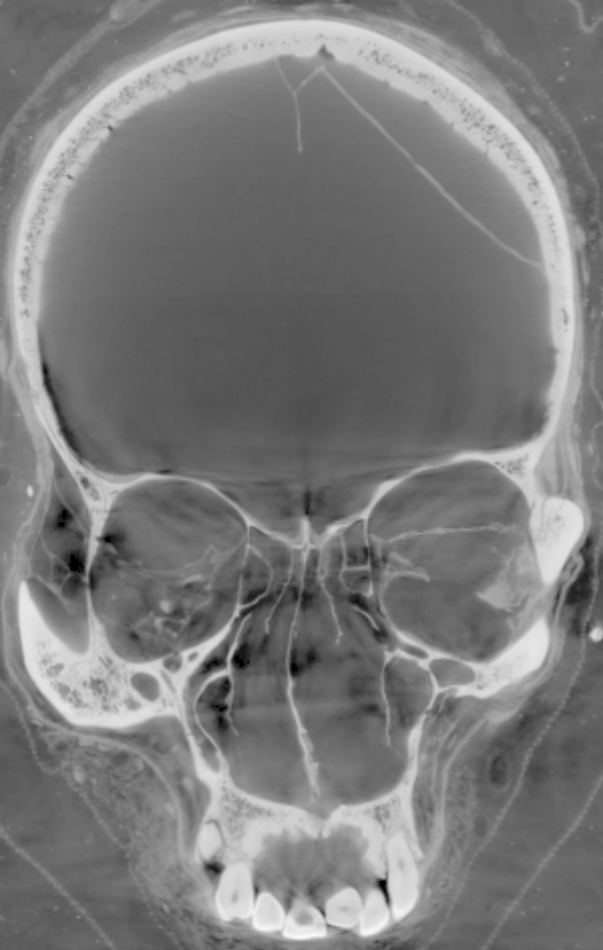
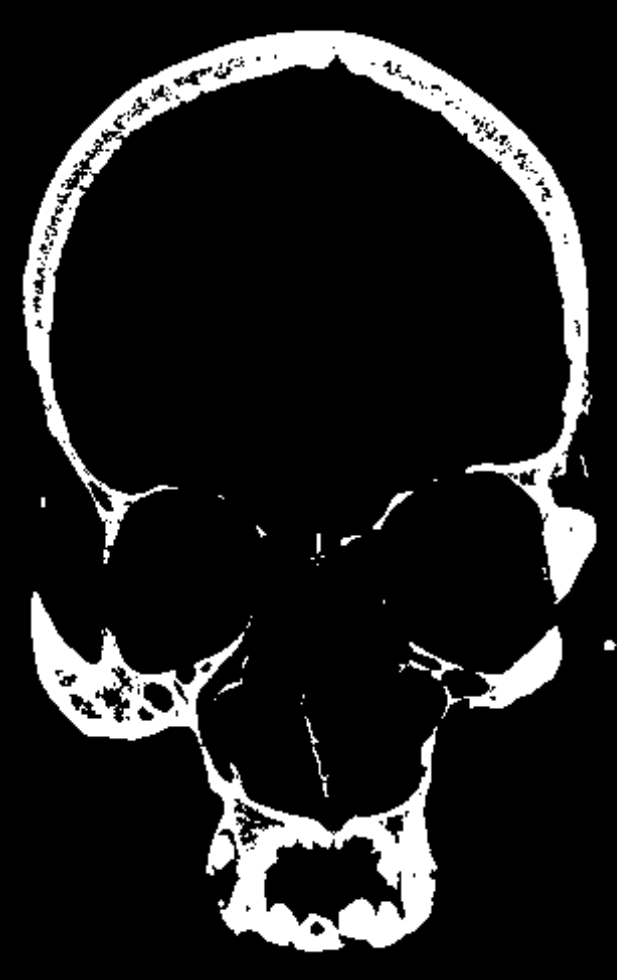
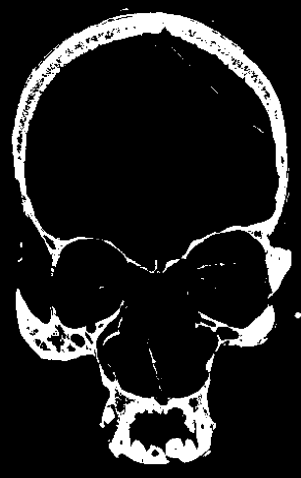
For surprisingly many applications this procedure is sufficient and it is perfectly applicable for big volumes since only information about the currently processed voxel is necessary for computing the result. However, especially in industrial computed tomography artifacts and physical effects frequently distort the grayscale values of certain parts of the object. In such regions, global thresholding is typically not able to capture the desired structure and thus produces “holes” there. An illustration of this effect is provided in Figure 1(c) which shows such holes at the top of the eye sockets of a skull. In those regions, a local binarizing threshold needs to be smaller than the global one, but if the global threshold would be adapted to a lower level, other parts of the volume would include mis-segmentations.

The paper is organized as follows. In Section 2, we briefly summarize existing approaches to adaptive thresholding, Section 3 introduces our model as an optimization problem and provides an algorithm for solving this problem and we motivate why our method is well suited for segmenting big voxel volumes. In Section 4 we apply our algorithm to selected datasets and demonstrate the improvement over plain thresholding. Finally, Section 5 summarizes our contributions.

2. Related Work

Of course, local thresholding itself is no new idea, notable examples include the techniques by Niblack [1] and Sauvola [2]. Both methods choose optimal binarizing thresholds in certain regions based on the local grayscale value distribution. However, in presence of high variance inside such regions, as it is often the case with measurement noise in industrial computed tomography, these methods compute a threshold which basically captures everything regardless of any structure. [3] computes a local threshold by comparing voxel values to the mean grayscale values in local regions and segments a voxel if it close enough to the average, while [4] computes local thresholds in overlapping regions using Rosin’s method, interpolates a high resolution threshold map and performs the pointwise comparison. On the other hand, [5] and [6] perform local thresholding by combining a global threshold with edge detection and morphological image processing to change the thresholding behavior locally. [7] computes a two-dimensional Dual Tree Complex Wavelet Transform for each volume slice and chooses local thresholds depending on the estimated noise level in order to reduce measurement noise. The work in [8] combines iterative image partitioning based on thresholds with local threshold estimation. Here, after one step of partitioning, a new local threshold is chosen from the grayscale value distribution for each partition based on which a new finer partitioning is found. An interesting yet computationally expensive approach was presented in [9]. There, the authors consider the thresholding process as a pixelwise functional which, after solving the according variational minimization problem, segments the image.

These approaches choose a threshold for each individual voxel. On the other hand, in practice a domain expert typically knows a good global threshold which is sufficient in most regions. Only few regions require a modified threshold in order to detect the structures as demonstrated in [10]. The idea of adapting a global threshold locally based on features was implemented in [11], where the authors aim for a local adaption based on planar structure detection. However, their approach requires two additional hyperparameters and an according tuning procedure while only planar features influence the result and other structures cannot be detected.

In order to overcome these limitations, our method focusses on allowing adaption by multiple features that can be chosen at will and problem-dependent and works without the need for feature-dependent hyperparameter tuning.

3. Local Thresholding as an Optimization Problem

Our method is based on and trained from user input that is provided interactively in such a way that several voxels are marked to identify critical regions where the threshold needs be adapted. Let $V$ be a volume of dimensions $\bm{d}$ as in Definition 1.1. Let $S\subseteq V$ be a set of seed voxels, selected at $M:=\#S\ll\#V$ critical positions. Around these voxels we extract local environments $U_{j}$, $j=1,\ldots,M$, of an application-dependent size $K\times K\times K$ where $K>1$ is odd. The size of the environments determines the features and depends on the image, in particular its resolution. By $F$ we denote the feature function which maps local environments onto a $d$-dimensional feature vector. Examples of such features can be found in [12]. In our application, $F$ is chosen depending on the dataset and includes structural information derived from the local distribution of grayscale values as well as geometric information encoding the similarity of local environments to primitives including lines and planes. It should be emphasized that any set of local features can be integrated in our approach. Finally, a global threshold $\theta_{g}\geq 0$ needs be provided which should be chosen such that it selects most of the object that shall be segmented – in plain words, it should be reasonable.

Within a local environment, we shall consider a local threshold.

Definition 3.1.

For $\theta_{g}\geq 0$ and weights $\bm{\beta}\in\mathbb{R}^{d}$, the (weighted) local threshold for a region $U$ is defined as

(2) $$\theta(U)=\theta_{g}+\bm{\beta}^{T}F(U).$$

Remark 3.1.

With mask-based processing, extracting a full voxel environment around each individual voxel becomes impossible at the borders of the volume. Classical workarounds include periodic extension, constant padding, repeating or mirroring the border voxel values or simply not processing them at all. In our application, we decided on the latter one and set the voxel values at the according positions explicitly zero.

We want to choose $\bm{\beta}$ such that the generated local thresholds are as close to optimal local thresholds in the critical regions. To that end, we first compute the features $F$ and estimate a local optimal binarizing threshold $\theta^{*}$ in the regions $U_{j}$, $j=1,\ldots,M$. In our concrete application, we specifically chose Minimum Cross Entropy Thresholding [13] for $\theta^{*}$, which basically computes the optimal threshold according to the cross entropy loss for binary classification using a histogram-based procedure. Putting everything together, we want our local thresholds to be close to the optimal ones given the parameters. To that end, define

$$\bm{\mathcal{F}}=\begin{bmatrix}F(U_{1})^{T}\\ \vdots\\ F(U_{M})^{T}\end{bmatrix}\quad\text{and}\quad\bm{\Theta}=\begin{bmatrix}\theta^{*}(U_{1})-\theta_{g}\\ \vdots\\ \theta^{*}(U_{M})-\theta_{g}\end{bmatrix},$$

and compute the optimal feature weights $\bm{\beta}$ as the solution of the minimization problem

$$\operatorname*{argmin}_{\bm{\beta}}\frac{1}{2}\|\bm{\mathcal{F}}\bm{\beta}-\bm{\Theta}\|_{2}^{2}.$$

To make the model more robust, we introduce elastic net regularization [14] to this least squares problem, see (3). This is known to reduce the risk of overfitting and only important features may adapt the threshold. A trade-off between both effects is achieved by tuning its hyperparameters $\lambda>0,\mu\in(0,1)$. Finally, we observe that so far we would deal with an unconstrained optimization problem. However, if the feature weights evolve in a way such that the produced local thresholds are always negative, we would segment every voxel regardless of our initial goal. To avoid this, we constrain the weights such that each local threshold is valid on the training regions. We call a threshold valid if it lies within the admissible grayscale interval $[0,W]$ where $W$ is the maximal representable voxel value depending on the data type, thus preventing thresholding with unreasonable values. In matrix form, define

$$\bm{C}=\begin{bmatrix}-\bm{\mathcal{F}}\\ \phantom{+}\bm{\mathcal{F}}\end{bmatrix}\quad\text{and}\quad\bm{b}=\begin{bmatrix}\;\;\phantom{(W-}\theta_{g}\bm{1}\\ (W-\theta_{g})\bm{1}\ \end{bmatrix}$$

which yields a closed convex polytope
$\mathcal{C}=\{\bm{x}\in\mathbb{R}^{d}\mid\bm{Cx}\leq\bm{b}\}$.

Our final optimization problem for finding the best feature weights is given as

(3) $$\begin{split}\operatorname*{argmin}_{\bm{\beta}}\quad&\frac{1}{2}\|\bm{\mathcal{F}\bm{\beta}}-\bm{\Theta}\|_{2}^{2}+\lambda\left(\frac{1-\mu}{2}\|\bm{\beta}\|_{2}^{2}+\mu\|\bm{\beta}\|_{1}\right)\\ s.t.\quad&\bm{C\bm{\beta}}\leq\bm{b}.\end{split}$$

3.1. Solving the Problem

We observe that the optimization problem (3) can be decomposed into

$$\operatorname*{argmin}_{\bm{\beta}}f(\bm{\beta})+g(\bm{\beta})+\iota_{\mathcal{C}}(\bm{\beta}),$$

where

$$f(\bm{\beta}) =\frac{1}{2}\|\bm{\mathcal{F}}\bm{\beta}-\bm{\Theta}\|_{2}^{2}+\frac{\lambda(1-\mu)}{2}\|\bm{\beta}\|_{2}^{2},$$

$$g(\bm{\beta}) =\lambda\mu\|\bm{\beta}\|_{1},$$

$$\iota_{\mathcal{C}}(\bm{\beta}) =\begin{cases}0,&\bm{\beta}\in\mathcal{C},\\ +\infty,&\text{otherwise}.\end{cases}$$

In this decomposition, the function $f$ is differentiable and convex while $g$ and $\iota_{\mathcal{C}}$ are convex. It is easy to see that all functions are proper and lower-semicontinuous as well. Therefore, the problem can be solved using the proximal gradients method, see [15]. To apply them on (3), we need explicit formulations of proximal operators which can then be interpreted as gradient steps for convex but nonsmooth functions. In the following, we will derive a proximal step for each of the three convex functions and combine them into a solver for (3).

3.1.1. The Individual Descent Steps

Since the convex function $f$ is differentiable, its gradient is given explicitly by

(4) $$\nabla f(\bm{x})=\bm{\mathcal{F}}^{T}\left(\bm{\mathcal{F}}\bm{x}-\bm{\Theta}\right)+\lambda(1-\mu)\bm{x},$$

which is linear and thus Lipschitz continuous in $x$.

Concerning the nonsmooth parts of our objective function, we consider their proximal operators, which, according to [15] are defined as

$$\operatorname{prox}_{h}(\bm{x})=\operatorname*{argmin}_{\bm{z}}\frac{1}{2}\|\bm{x}-\bm{z}\|_{2}^{2}+h(\bm{z})$$

for a proper lower-semicontinuous function $h$. For our particular function $g$, it is known that the according proximal operator is a scaled soft-thresholding function, cf. [16].

Definition 3.2.

For $\theta\geq 0$, define soft-thresholding with respect to $\theta$ as

$$S_{\theta}\colon\mathbb{R} \to\mathbb{R},$$

$$x \mapsto\operatorname{sgn}(x)\,\max\{0,|x|-\theta\}.$$

For the indicator function $\iota_{\mathcal{C}}$, on the other hand, the associated proximal operator is given by the projection onto the polytope $\mathcal{C}$ since

$$\operatorname{prox}_{\iota_{\mathcal{C}}}(\bm{x}) =\operatorname*{argmin}_{\bm{z}}\frac{1}{2}\|\bm{x}-\bm{z}\|_{2}^{2}+\iota_{\mathcal{C}}(\bm{z})$$

$$=\operatorname*{argmin}_{\bm{z}\in\mathcal{C}}\frac{1}{2}\|\bm{x}-\bm{z}\|_{2}^{2}=\mathcal{P_{C}}(\bm{x}).$$

In lack of a closed-form solution for the projection onto a convex polytope in general, we use Hildreth’s method for inequalities [17, p. 283] to compute the projection iteratively.

3.1.2. Choosing the step size

The final ingredient to iteratively train the FAITH model is the step size whose choice it is a well-discussed topic in literature. This includes constant step size, finding the best one in each iteration by a line search [18] or accelerations including momentum methods [19]. For simplicity, we choose a constant step size $\delta=L^{-1}$ where $L$ denotes a Lipschitz constant of the gradient of $f$, but we emphasize that our method can also be enhanced with the techniques mentioned above.

By (4), we have that

$$\|\nabla f(\bm{x})-\nabla f(\bm{y})\|\leq\|\bm{\mathcal{F}}^{T}\bm{\mathcal{F}}+\lambda(1-\mu)\bm{I}\|_{2}\|\bm{x}-\bm{y}\|.$$

Since adding a nonnegative multiple of the identity matrix to the positive semidefinite $\bm{\mathcal{F}}^{T}\bm{\mathcal{F}}$ only shifts the eigenvalues, we note that $\|\bm{\mathcal{F}}^{T}\bm{\mathcal{F}}+\lambda(1-\mu)\bm{I}\|_{2}=\|\bm{\mathcal{F}}^{T}\bm{\mathcal{F}}\|_{2}+\lambda(1-\mu)$ and consequently

$$\|\bm{\mathcal{F}}^{T}\bm{\mathcal{F}}+\lambda(1 -\mu)\bm{I}\|_{2}\|\bm{x}-\bm{y}\|$$

$$=\left(\|\bm{\mathcal{F}}^{T}\bm{\mathcal{F}}\|_{2}+\lambda(1-\mu)\|\bm{I}\|_{2}\right)\|\bm{x}-\bm{y}\|$$

$$=\underbrace{\left(\operatorname{Eig}_{\max}(\bm{\mathcal{F}}^{T}\bm{\mathcal{F}})+\lambda(1-\mu)\right)}_{=:L}\|\bm{x}-\bm{y}\|,$$

where $\operatorname{Eig}_{\max}$ denotes the maximal eigenvalue of its argument matrix. Note that $L>0$ since $\bm{\mathcal{F}}^{T}\bm{\mathcal{F}}$ is positive semi-definite and $\lambda>0$ and $0<\mu<1$ holds.

3.1.3. Putting it Together

The basic proximal gradient method employs forward-backward splitting [16] which performs a gradient descent step for the differentiable part and a proximal step for the nonsmooth part. Motivated this idea, one may be tempted to pursue a forward-backward-backward iteration of the form

$$\begin{cases}\bm{\beta}^{(0)}\in\mathbb{R}^{d},&\\ \bm{\beta}^{(k+1)}=\mathcal{P_{C}}\left(S_{\delta\lambda\mu}\left(\bm{\beta}^{(k)}-\delta\nabla f\left(\bm{\beta}^{(k)}\right)\right)\right).&\end{cases}$$

While this iteration converges linearly to a unique fixed point, the solution obtained this way is not necessarily the optimal solution of Problem (3). This can only be guaranteed provided that

(5) $$\operatorname{prox}_{\delta\iota_{\mathcal{C}}+\delta g}=\operatorname{prox}_{\delta\iota_{\mathcal{C}}}\circ\operatorname{prox}_{\delta g}$$

is fulfilled, in which case the following equivalences hold:

$$0 \in\nabla f(\bm{x}^{*})+\partial g(\bm{x}^{*})+\partial\iota_{\mathcal{C}}(\bm{x}^{*})$$

$$\Leftrightarrow\;\bm{x}^{*} =\operatorname{prox}_{\delta\iota_{\mathcal{C}}+\delta g}\left(\bm{x}^{*}-\delta\nabla f(\bm{x}^{*})\right)$$

$$\Leftrightarrow\;\bm{x}^{*} =\left(\operatorname{prox}_{\delta\iota_{\mathcal{C}}}\circ\operatorname{prox}_{\delta g}\right)\left(\bm{x}^{*}-\delta\nabla f(\bm{x}^{*})\right)$$

$$\Leftrightarrow\;\bm{x}^{*} =\mathcal{P}_{\mathcal{C}}\left(S_{\delta\lambda\mu}\left(\bm{x}^{*}-\delta\nabla f(\bm{x}^{*})\right)\right)$$

Then, the naive fixpoint iteration converges and the fixpoint is an optimal solution to our problem. However, (5) is not always fulfilled. For a counterexample, consider $\mathcal{C}=\{(x,y)^{T}\in\mathbb{R}^{2}\mid y\leq-2x\}$, $\bm{\mathcal{F}}=\bm{I}$, $\bm{\Theta}=(1,3)^{T}$, $\lambda=1$ and $\mu=1/2$. Let $\bm{p}=(1,3)^{T}$. Then, $\delta=L^{-1}=2/3$ and we observe that

$$\operatorname{prox}_{\iota_{\mathcal{C}}+g}(\bm{p})=\begin{bmatrix}-0.4\\ 0.8\end{bmatrix}\neq\begin{bmatrix}-0.9\\ 1.9\end{bmatrix}=\operatorname{prox}_{\iota_{\mathcal{C}}}\left(\operatorname{prox}_{g}(\bm{p})\right).$$

To avoid this problem, we incorporate a nested optimization scheme as introduced in [20], and choose the following parameters:

• $(\gamma_{n})_{n\in\mathbb{N}}=\delta=L^{-1}$ with $L$ as above

• $(\lambda_{n})_{n\in\mathbb{N}}=1$

• $\tau=1$

The procedure is summarized in Algorithm 1. We say that the algorithm has converged if the weights $\bm{\beta}$ become stationary, i.e., if $\|\bm{\beta}^{(k+1)}-\bm{\beta}^{(k)}\|_{2}<\epsilon$ for a small positive number $\epsilon$.

Function FAITH_Training($\bm{\mathcal{F}}$, $\theta_{g}$, $\lambda$, $\mu$)

       Input : Feature matrix $\bm{\mathcal{F}}\in\mathbb{R}^{M\times d}$

      from seed voxel selection

       Input : Global threshold $\theta_{g}\geq 0$

       Input : Regularization parameters $\lambda>0,\mu\in(0,1)$

       Output : Feature weight vector $\bm{\beta}\in\mathbb{R}^{d}$

       $\bm{C}\leftarrow\begin{bmatrix}-\bm{\mathcal{F}}\\ \phantom{+}\bm{\mathcal{F}}\end{bmatrix}$

       $\bm{b}\leftarrow\begin{bmatrix}\;\;\phantom{(W-}\theta_{g}\bm{1}\\ (W-\theta_{g})\bm{1}\ \end{bmatrix}$

       $\delta\leftarrow\left(\operatorname{Eig}_{\max}(\bm{\mathcal{F}}^{T}\bm{\mathcal{F}})+\lambda(1-\mu)\right)^{-1}$

       $\bm{\beta}\leftarrow\bm{0}$

       while $\bm{\beta}$ not converged do

             $\bm{x}\leftarrow\bm{\beta}-\delta\nabla f(\bm{\beta})$

             $\bm{z}\leftarrow 2S_{\delta\lambda\mu}(\bm{x})-\bm{x}$

             while $\bm{z}$ not converged do

                   $\hat{\bm{z}}\leftarrow\mathcal{P_{C}}\left(\frac{1}{2}(\bm{z}+\bm{x})\right)$

                   $\bm{z}\leftarrow\bm{z}+S_{\delta\lambda\mu}(2\hat{\bm{z}}-\bm{z})-\hat{\bm{z}}$

                  

            $\bm{\beta}\leftarrow\hat{\bm{z}}$

              // The last value of $\hat{\bm{z}}$

            

      return $\bm{\beta}$

      

Algorithm 1 Iterative solver for Problem (3).

Using the techniques from [20, Proposition 4.2] and taking that the polytope $\mathcal{C}$ is always nonempty as it contains at least the feasible point $\bm{0}$, the nested iteration can be shown in a straightforward way to converge to the optimal solution.

Theorem 3.1.

The sequence $\bm{\beta}^{(k)}$ generated by Algorithm 1 converges to a solution of (3).

3.2. Hyperparameter Tuning

Our thresholding model contains two hyperparameters, i.e., parameters not optimized by the solver, namely, the regularization parameters $\lambda>0$ and $\mu\in(0,1)$. In order to tweak them we use a Grid Search approach.

The hyperparameter $\mu$ controls the trade-off between sparsity and smoothness. The closer $\mu$ approaches $1$, the more focus is laid on sparsity while denser solutions are obtained as $\mu$ becomes zero. In the practical application we use the discrete parameter set $P_{\mu}=\{0.25,0.33,0.42,0.50,0.58,0.67,0.75\}$ and omit $\mu=1$ in order to avoid singularities during the computation of the step size $\delta$.

Regarding $\lambda$ we apply the approach presented in [21] where the maximum meaningful value is given by $\lambda_{\max}(\mu)=\mu^{-1}\|\bm{\mathcal{F}}^{T}\bm{\Theta}\|_{2}$. Then, a regularization path is constructed in log-space resulting in the parameter set $P_{\lambda}=\{\epsilon\lambda_{\max}(\mu)10^{\frac{k}{k_{\max}-1}\log_{10}(\epsilon^{-1})}\}_{k=0}^{k_{\max}-1}$ containing $k_{\max}$ values. Experimentally, we used $k_{\max}=16$ and a small $\epsilon>0$.

The overall hyperparameter grid is given as $P=P_{\lambda}\times P_{\mu}$. In our application, we used $K$-fold cross validation to select the best parameters out of this fixed set.

3.3. Segmenting Big Volumes

Based on the training procedure, we can now formulate a segmentation procedure. To that end, we consider an input volume of dimensions $\bm{d}\in\mathbb{N}^{3}$ with voxels at positions $\bm{\alpha}\leq\bm{d}$ and an output volume of identical dimensions with voxel values $\widetilde{x}_{\bm{\alpha}}$. The method is outlined in Algorithm 2. We assume that a user, ideally domain expert, interactively selected $M$ seed voxels in critical regions $U_{1},\dots,U_{M}$ and furthermore provided a global threshold $\theta_{g}$ that binarizes most of the components under investigation well. Depending on the actual application, the user may also provide a selection of (geometric) features to use, but they could also be determined automatically, cf. [12]. In the first step, we extract local environments around the selected seed voxels and compute the feature vectors on these regions to build the feature matrix $\bm{\mathcal{F}}$. Then, a grid search determines the best pair of hyperparameters which is used for training our FAITH model and obtaining feature weights $\bm{\beta}$.

Finally, for the eventual segmentation we iterate (possibly in parallel) over the input volume. For each voxel we extract a local voxel environment around it and compute the same set of features with proper handling of boundary voxels, cf. Remark 3.1. The result is combined with the trained feature weights and the global threshold in order to compute a localized threshold $\theta$. The value of the voxel in the target volume at the same position as the input volume is given as the result of binarizing thresholding with that local threshold.

Function FAITH_Segmentation($V,S,K,F,\theta_{g}$)

       Input : Input volume $V$

       Input : Seed voxel collection $S\subseteq V$, $\#S=M$

       Input : Environment size $K\in 2\mathbb{N}+1$

       Input : Feature computation function $F$

       Input : Global threshold $\theta_{g}\geq 0$

       Output : Output volume $\widetilde{V}$

       $\{U_{j}\}_{j=1}^{M}\leftarrow$ extract $K\times K\times K$ environment

            around seed voxels $S$

       $\bm{\mathcal{F}}\leftarrow\begin{bmatrix}F(U_{1})\\ \vdots\\ F(U_{M})\end{bmatrix}$

       $(\lambda^{*},\mu^{*})\leftarrow$ determine by grid search

       $\bm{\beta}\leftarrow$ FAITH_Training($\bm{\mathcal{F}},\theta_{g},\lambda^{*},\mu^{*}$)

       for $\bm{\alpha}$ in $V$ do

             $U\leftarrow$ $K\times K\times K$ environment around $\bm{\alpha}$

             $\theta\leftarrow\theta_{g}+\bm{\beta}^{T}F(U)$

             $\widetilde{x}_{\bm{\alpha}}\leftarrow T_{\theta}(x_{\bm{\alpha}})$

            

      

Algorithm 2 Segmentation using FAITH

3.4. Runtime and Memory Analysis

For large voxel volumes, only algorithms with linear runtime in the number of voxels are admissible in practice. Therefore, we briefly analyze the runtime and memory requirements of our thresholding procedure.

Concerning the runtime, the extraction of local environments around the seed voxels has a runtime of $\mathcal{O}(M)$ where $M$ denotes the number of seed voxels. The training itself consists of a nested solver loop with $m$ iterations of the outer loop and $k_{j},j=1,\ldots,m$, the associated inner iterations. With $k=\sum_{j=1}^{m}k_{j}$, a single FAITH training has a runtime complexity of $\mathcal{O}(k)$. Each iteration depends on the number of seed voxels $M$ in some polynomial way, however since $M$ is typically very small and, more important, independent of the number of voxels in the volume, the according factor will be so as well. Aggregating the runtimes of the training involving a grid search over $\#P$ parameters using $t$ threads and the last training with the found hyperparameters, we obtain $\mathcal{O}(k(1+\frac{\#P}{t}))$. The final step involves a single pass through the voxel volume which is clearly linear in the number $N$ of voxels.

Overall, the runtime complexity of Algorithm 2 can thus be estimated as

$$\mathcal{O}\left(M+k\left(1+\frac{\#P}{t}\right)+N\right).$$

Already for practical reasons, the number of seed voxels $M$ is typically very small (since they have to be marked manually) and independent of $N$, thus asymptotically yielding an effort which is linear with respect to the number of voxels $N$.

Considering memory requirements, we notice that during training we need to keep the feature matrix, the polytope constraints and of course the solution vector in memory. The feature matrix $\bm{\mathcal{F}}$ is of size $M\times d$, where $d$ is the dimensionality of the feature vector. Likewise, the polytope constraints consist of a matrix $\bm{C}$ of size $2M\times d$ and a vector $\bm{b}$ of size $2M$. The solution vector $\bm{\beta}$ has dimensionality $d$. Thus, the overall space complexity for training scales with $Md$. The classification phase only relies on local environments of fixed size and the trained solution vector, thus having constant memory complexity. Fortunately, the feature vector dimensionality is constant after feature selection and thus the memory requirements scale linearly with the number of seed voxels which is assumed independent of the number of voxels, making our segmentation procedure especially well suited for handling large three-dimensional datasets.

4. Results

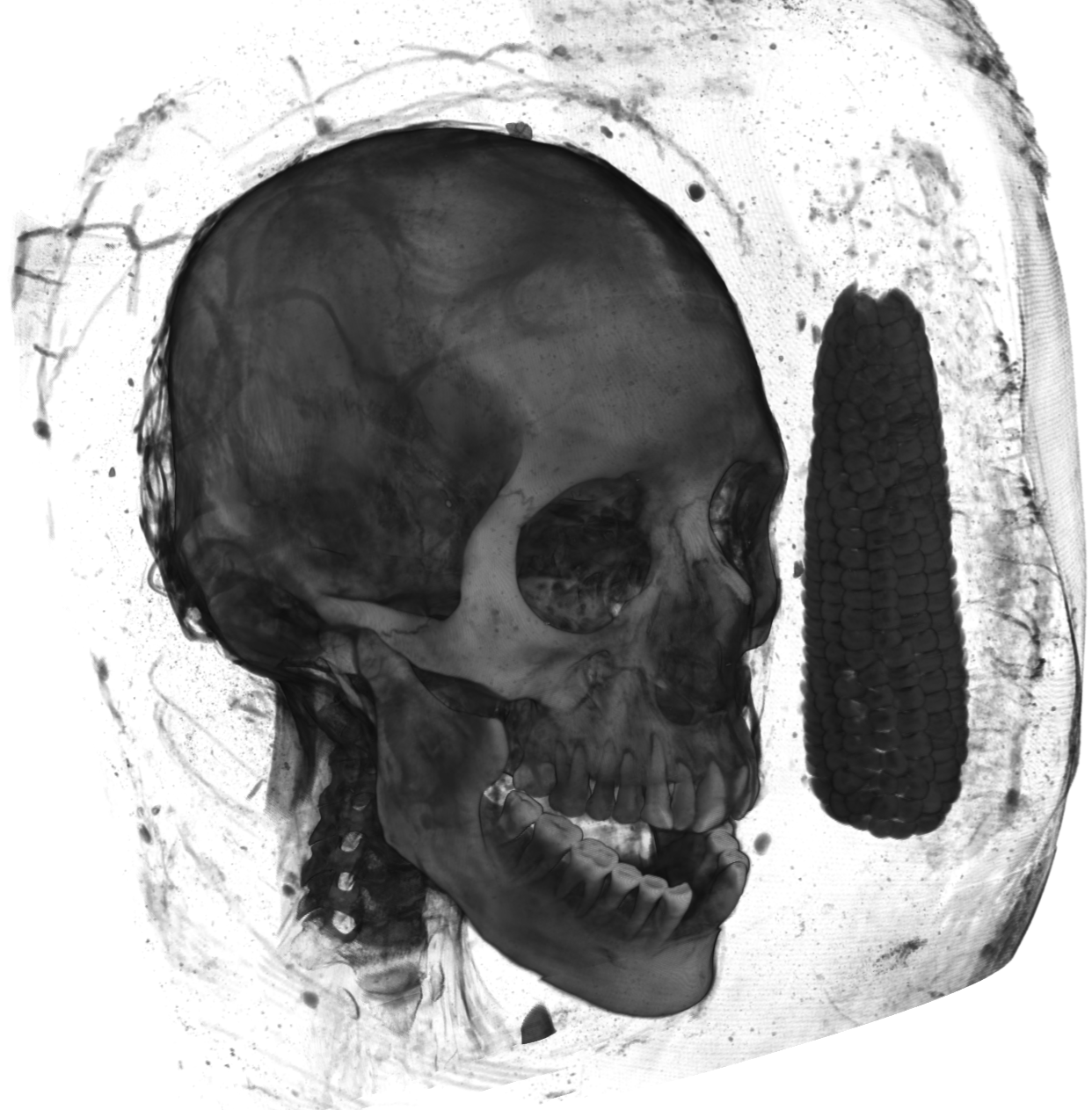
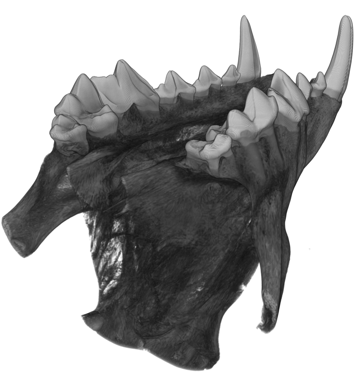
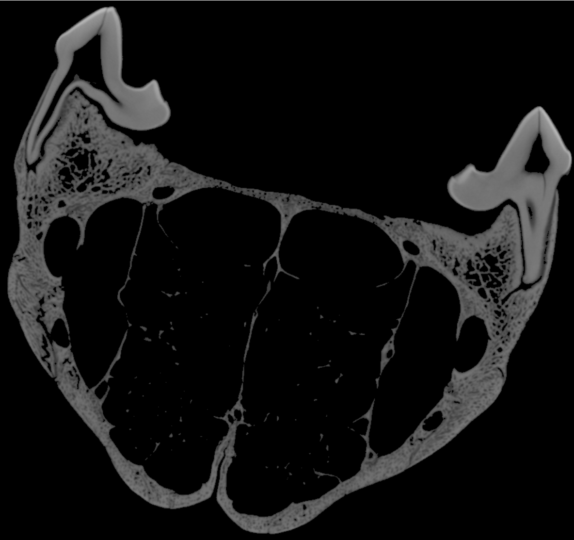
In this section we demonstrate the capabilities of our algorithm to detect geometric structures not captured by global thresholding by means of two examles. Figure 1(a) shows a rendering of the head section of a Peruvian mummy now located at the Lindenmuseum in Stuttgart, while Figure 3(a) shows a computed tomography scan of a wolf jaw labeled ”Canis Lupus”. Both scans were generated by the Fraunhofer Development Center for X-ray Technology in Fürth.

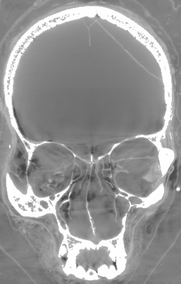
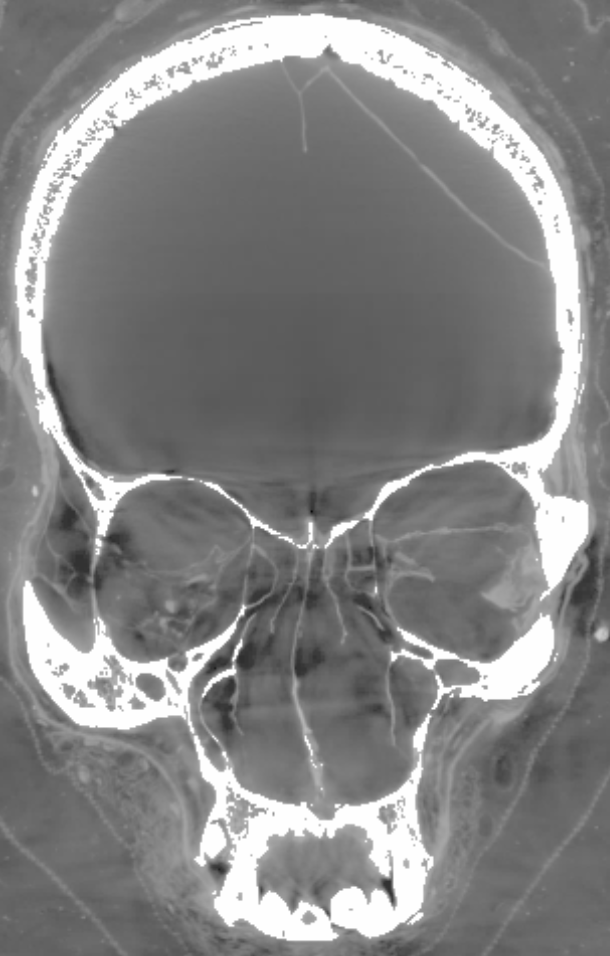
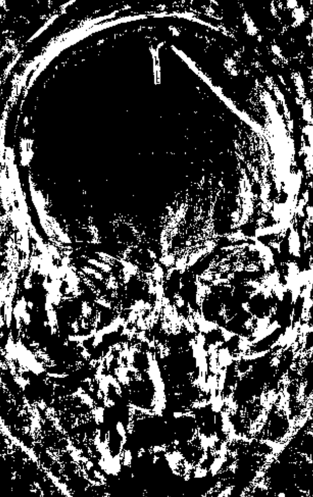
Our first aim was to segment the skull of the mummy without capturing the wrappings around it. Doing so, we used the global threshold specified in Table 1. In Figure 1(c) we see that global thresholding results in holes at the top of the eye sockets, whereas lowering that threshold would result in segmenting the wrappings too. We applied FAITH by interactively selecting 54 seeds out of 104,368,576 total voxels in these critical regions and set the parameters as in Table 1, using the same global threshold. The result is given in Figure 1(d) with a clearly visible improvement in the critical regions. At the same time, the rest of the skull which was detected properly by the global threshold stays unaffected. Thus, the planar structures of the eye socket are detected by the features quite well and the segmentation result improved considerably. As a side note we like to demonstrate the influence of our modifications to the basic least squares approximation. The differences can be observed in Figure 2. The least squares problem without regularization is rendered ill-conditioned if a feature produces the very same values for multiple environments, resulting in a volume cluttered with missegmentations. Regularization and restricting to valid thresholds improves this to the known result.

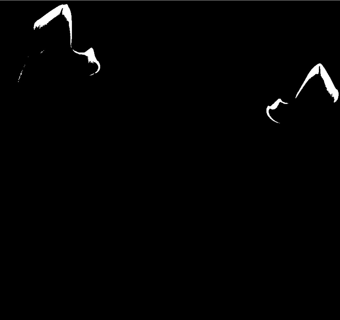
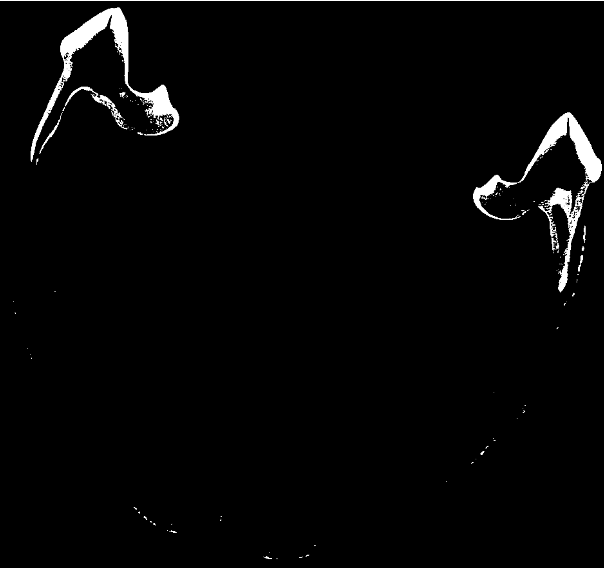
We also applied our procedure to the wolf jaw scan. Here, we specified the threshold in a way such that the teeth are kept as good as possible, while the jaw bone shall be discarded. Unfortunately, binarization using a global threshold also discards most of the teeth, cf. Figure 3(c). Again, we interactively selected critical regions, set the FAITH parameters as specified in Table 1 and applied the segmentation method. Here, we selected 166 out of 2,467,050,300 total voxels. The result is depicted in Figure 3(d) in which the teeth are detected better. While individual voxels of the jaw bone remain, these can be easily removed by simple postprocessing.

The execution times of these applications are summarized in Table 2. The implementation is within a Fraunhofer software framework and runs exclusively on the CPU; the measurements were recorded on an Intel^® Core^™ i7-770H processor with eight logical cores and an average clock rate of 4.2 GHz. While the procedure is algorithmically efficient in the sense that its runtime is linear with respect to the number of voxels, the cubic increase of the number of voxels with respect to resolution makes us propose that in future work this algorithm should be implemented on GPUs to accelerate this even further.

Scan	Threshold	Env. size	#Features
Canis Lupus	24415	5	2
Mummy skull	1541	7

Table 1. Experiment setup

Scan	Size	Time
Mummy skull	199 MiB	1801.79 s
Canis Lupus	4076 MiB	3155.80 s

Table 2. Runtime measurements

(a) Mummy head

(b) Original data

(c) Binarization

(d) FAITH

Figure 1. Binarization applied to the mummy skull data in (1(b)) produces holes at the top of the eye sockets (1(c)). FAITH is able to detect bone in these critical sections while the overall segmentation remains good (1(d)). Results are overlaid in white over the original data.

(a) Binarization

(b) Least Squares only

(c) FAITH

Figure 2. Applying global binarization fails to detect bone in the upper eye socket regions (2(a)). FAITH without any kind of regularization and validity constraints, i.e., using only a simple least squares approximation, produces a very cluttered result (2(b)). The full procedure omits these problems and shows the better segmented skull in (2(c)).

(a) Wolf jaw

(b) Original data

(c) Binarization

(d) FAITH

Figure 3. Binarization applied to a scan of wolf jaw labeled Canis Lupus in (3(b)) discards most of the teeth structure, see (3(c)). Our procedure detects the teeth better while simultaneously discarding the jaw bone we wish to ignore (1(d)).

5. Conclusions

In this work we proposed FAITH, a novel thresholding technique which adapts a global threshold locally on the basis of freely selectable features. The main benefit is that a domain expert can interactively identify critical regions where global thresholding produces undesirable results. Inside these regions, features extract structural information and a model is trained to modify the global threshold in a way such that the localized threshold is optimal inside these regions. At the same time, the global one is modified only if the trained structure is observed, thus in regions where the global threshold suffices for segmentation, the detection quality remains the same. Overall, this procedure allows improving the segmentation quality over global thresholding interactively and at the same time handling three-dimensional datasets without size restrictions due to purely local processing. Furthermore, the same algorithm can be used for a variety of different domains and applications as long as we process volumes and the object under investigation can be segmented using a thresholding approach.

Acknowledgements This work was supported by the project ”Digitalisierung, Verarbeitung und Analyse kultureller und industrieller Objekte: Wertschöpfung aus großen Daten und Datenmengen - Big Picture” that has been promoted and funded by the Bavarian State Government under Grant No. AZ.: 43-6623/138/2 from 2018 to 2021.

References

- [1] W. Niblack, An Introduction to Digital Image Processing. Birkeroed, Denmark, Denmark: Strandberg Publishing Company, 1985.
- [2] J. Sauvola and M. Pietikäinen, “Adaptive document image binarization,” Pattern Recognit., vol. 33, no. 2, pp. 225–236, 2000.
- [3] D. Bradley and G. Roth, “Adaptive Thresholding using the Integral Image,” J. Graph. Tools, vol. 12, pp. 13–21, 01 2007.
- [4] J. Lifton and T. Liu, “An adaptive thresholding algorithm for porosity measurement of additively manufactured metal test samples via X-ray computed tomography,” Addit. Manuf., vol. 39, p. 101899, 2021.
- [5] A. J. Burghardt, G. J. Kazakia, and S. Majumdar, “A Local Adaptive Thresholding Strategy for High Resolution Peripheral Quantitative Computed Tomography of Trabecular Bone,” Ann. Biomed. Eng., vol. 35, no. 10, pp. 1678–1686, 2007.
- [6] J. Kittler, J. Illingworth, and J. Föglein, “Threshold selection based on a simple image statistic,” Comput. Vis. Graph. Image Process., vol. 30, no. 2, pp. 125–147, 1985.
- [7] M. Diwakar, Sonam, and M. Kumar, “CT Image Denoising Based on Complex Wavelet Transform Using Local Adaptive Thresholding and Bilateral Filtering,” in Proceedings of the Third International Symposium on Women in Computing and Informatics, ser. WCI ’15, 2015, pp. 297––302.
- [8] D. Y. Kim and J. W. Park, “Connectivity-Based Local Adaptive Thresholding for Carotid Artery Segmentation Using MRA Images,” Image Vis. Comput., vol. 23, no. 14, pp. 1277––1287, 12 2005.
- [9] F. H. Chan, F. Lam, and H. Zhu, “Adaptive Thresholding by Variational Method,” IEEE Trans. Image Process., vol. 7, no. 3, pp. 468–473, 1998.
- [10] J. Michetti, A. Basarab, F. Diemer, and D. Kouame, “Comparison of an adaptive local thresholding method on CBCT and CT endodontic images,” Phys. Med. Biol., vol. 63, no. 1, p. 015020, 2017.
- [11] C.-F. Westin, A. Bhalerao, H. Knutsson, and R. Kikinis, “Using Local 3D Structure for Segmentation of Bone from Computer Tomography Images,” in CVPR, 06 1997, pp. 794–800.
- [12] T. Lang, “AI-Supported Interactive Segmentation of 3D Volumes,” Ph.D. dissertation, University of Passau, 07 2021.
- [13] C. Li and C. Lee, “Minimum cross entropy thresholding,” Pattern Recognit., vol. 26, no. 4, pp. 617 – 625, 1993.
- [14] H. Zou and T. Hastie, “Regularization and variable selection via the elastic net,” J. R. Stat. Soc., Series B, vol. 67, pp. 301–320, 2005.
- [15] N. Parikh and S. Boyd, “Proximal Algorithms,” Found. Trends Optim., vol. 1, no. 3, pp. 127–239, 01 2014.
- [16] P. Combettes and V. R. Wajs, “Signal Recovery by Proximal Forward-Backward Splitting,” Multiscale Model Simul., vol. 4, 01 2005.
- [17] G. T. Herman and A. Lent, “Iterative reconstruction algorithms,” Comput. Biol. Med., vol. 6, no. 4, pp. 273–294, 1976.
- [18] S. Boyd and L. Vandenberghe, Convex Optimization. Cambridge University Press, 03 2004.
- [19] D. E. Rumelhart, G. E. Hinton, and R. J. Williams, Learning Representations by Back-Propagating Errors. Cambridge, MA, USA: MIT Press, 1988, p. 696–699.
- [20] C. Chaux, J.-C. Pesquet, and N. Pustelnik, “Nested Iterative Algorithms for Convex Constrained Image Recovery Problems,” SIAM J. Imaging Sci., vol. 2, no. 2, pp. 730–762, 2009.
- [21] R. Tibshirani, T. Hastie, and J. Friedman, “Regularized Paths for Generalized Linear Models Via Coordinate Descent,” J. Stat. Softw., vol. 33, 02 2010.