EUROPEAN ORGANIZATION FOR NUCLEAR RESEARCH (CERN)

​​​ CERN-EP-2022-148 LHCb-PAPER-2021-046 13 October 2022

Measurement of the ${\mathchar 28931\relax}^{+}_{c}$ to ${D}^{0}$ production ratio in peripheral $\mathrm{Pb}\mathrm{Pb}$

collisions at $\sqrt{s_{\scriptscriptstyle\text{NN}}}$ = 5.02 TeV

LHCb collaboration

We report on a measurement of the ${\mathchar 28931\relax}^{+}_{c}$ to ${D}^{0}$ production ratio in PbPb collisions at $\sqrt{s_{\scriptscriptstyle\text{NN}}}$ = 5.02 TeV with the LHCb detector in the forward rapidity region $2<y<4.5$. The ${\mathchar 28931\relax}^{+}_{c}$ (${D}^{0}$) hadrons are reconstructed via the decay channel ${{\mathchar 28931\relax}^{+}_{c}}\rightarrow p{{K}^{+}}{{\pi}^{-}}$ (${{D}^{0}}\rightarrow{{K}^{-}}{{\pi}^{+}}$) for $2<p_{\mathrm{T}}<8$ $\text{\,Ge\kern-1.00006ptV\!/}c$ and in the centrality range of about 65–90%. The results show no significant dependence on $p_{\mathrm{T}}$, $y$ or the mean number of participating nucleons. They are also consistent with similar measurements obtained by the LHCb collaboration in pPb and Pbp collisions at $\sqrt{s_{\scriptscriptstyle\text{NN}}}$ = 5.02 TeV. The data agree well with predictions from PYTHIA in pp collisions at $\sqrt{s}$ = 5  TeV but are in tension with predictions of the Statistical Hadronization model.

Submitted to JHEP

© 2024 CERN for the benefit of the LHCb collaboration. CC BY 4.0 licence.

 

1 Introduction

Historically, heavy flavor ($\mathrm{HF}$) hadrons have been extensively used to study the deconfined state of hadronic matter, the Quark-Gluon Plasma ($\mathrm{QGP}$) [1, 2, 3], in particular at the LHC and RHIC [4, 5]. Because of their high masses exceeding the QCD energy scale, $\mathrm{HF}$ are produced at an early stage of the collision and experience the full evolution of the colliding medium. Medium-induced energy loss has been studied by measuring the so-called nuclear modification factor ($R_{\rm AA}$), defined as the ratio of the production yield in nucleus-nucleus (AA) collisions to the one in $p$ $p$ collisions scaled by the number of binary nucleon-nucleon collisions. The measurements of the production cross-section, together with studies of the elliptic flow, indicate a strong interaction between $\mathrm{HF}$ and the deconfined medium.

In addition, $\mathrm{HF}$ hadrons provide a good laboratory to study hadronization. In particular, baryon-to-meson production ratios are of great interest as they are only sensitive to hadronization. Many measurements have been carried on in $e^{+}e^{-}$ [6, 7, 8] and $p$ $p$ collisions [9, 10, 11] to measure fragmentation functions of heavy hadrons, the latter being extensively used to describe hadron production at high transverse momentum ($p_{\mathrm{T}}$). However, recent measurements of the ${\mathchar 28931\relax}^{+}_{c}$ to ${D}^{0}$ production ratio ($R_{{{\mathchar 28931\relax}^{+}_{c}}/{{D}^{0}}}$) challenge understanding of hadronization. At the LHC, ALICE has measured the charmed baryon-to-meson ratio at mid-rapidity in $p$ $p$, ${p}\mathrm{Pb}$ and $\mathrm{Pb}\mathrm{Pb}$ collisions at $\sqrt{s}$ = 7 TeV and $\sqrt{s_{\scriptscriptstyle\text{NN}}}$ = 5.02 TeV, respectively [12, 13, 14]. An enhancement compared to predictions of the $p$ $p$ event generator PYTHIA 8 [15] without the color reconnection (CR) mechanism is found both in $p$ $p$ and ${p}\mathrm{Pb}$ data at low $p_{\mathrm{T}}$. The $\mathrm{Pb}\mathrm{Pb}$ result, obtained for $p_{\mathrm{T}}$ $>$ 6 $\text{\,Ge\kern-1.00006ptV\!/}c$, is compatible with various theory models [16] predicting a large enhancement of the ratio compared to $p$ $p$ and ${p}\mathrm{Pb}$ collisions. Similarly, CMS [17] has performed the same measurement at mid-rapidity in $p$ $p$ and $\mathrm{Pb}\mathrm{Pb}$ collisions at $\sqrt{s_{\scriptscriptstyle\text{NN}}}=5.02\text{\,Te\kern-1.00006ptV}$, for $p_{\mathrm{T}}$ $>$ 5 $\text{\,Ge\kern-1.00006ptV\!/}c$. In this case the data are well described by PYTHIA 8 only when the CR mechanism is allowed. At the RHIC collider, the STAR collaboration has also measured $R_{{{\mathchar 28931\relax}^{+}_{c}}/{{D}^{0}}}$ at mid-rapidity in Au-Au collisions at $\sqrt{s_{\scriptscriptstyle\text{NN}}}$ = 200  GeV [18]. An enhanced baryon-to-meson ratio is found at low $p_{\mathrm{T}}$ compared to scaled $p$ $p$ collisions. It is worth mentioning that both ALICE and STAR measurements in AA collisions can be described by a coalescence hadronization mechanism [19, 16] in which quarks can (re)combine with close-by partons in the $\mathrm{QGP}$ to form hadrons. Other predictions based on the Statistical Hadronization Model (SHM) [20, 21] have successfully described the charmed baryon-to-meson ratio measured at RHIC and LHC.

As mentioned, ALICE, CMS and STAR measure a $R_{{{\mathchar 28931\relax}^{+}_{c}}/{{D}^{0}}}$ in heavy-ion collisions at mid-rapidity, with raising trend from low to intermediate transverse momentum. On the other hand, LHCb has measured a ratio with no $p_{\mathrm{T}}$ dependence in ${p}\mathrm{Pb}$ collisions at $\sqrt{s_{\scriptscriptstyle\text{NN}}}=5.02\text{\,Te\kern-1.00006ptV}$ in the rapidity range $2<y<4.5$ [22].These results correspond to smaller $R_{{{\mathchar 28931\relax}^{+}_{c}}/{{D}^{0}}}$ values compared to measurements by other experiments, and are fully compatible with predictions from cold nuclear matter effects [23, 24]. The LHCb results are yet to be compared with a coalescence based model. These differences between mid and forward rapidity results indicate a strong rapidity dependence of this ratio, and motivate further studies to better improve the model predictions in different phase-space regions.

This paper presents the first measurement of $R_{{{\mathchar 28931\relax}^{+}_{c}}/{{D}^{0}}}$ production cross-section ratio in the forward rapidity region in peripheral $\mathrm{Pb}\mathrm{Pb}$ collisions at $\sqrt{s_{\scriptscriptstyle\text{NN}}}$ = 5.02 TeV by the LHCb collaboration. The paper is organized as follows. Section 2 briefly presents the detector and the data sample. Section 3 describes the analysis steps, from the signal extraction to the estimation of efficiency corrections. The sources of systematic uncertainties are given in Sec. 4. The results are presented and compared to theory predictions in Sec. 5, and conclusions are summarized in Sec. 6.

2 Detector and data selection

The LHCb detector [25, 26] is a single-arm forward spectrometer covering the pseudorapidity range $2<\eta<5$, designed for the study of particles containing $b$ or $c$ quarks. The detector includes a high-precision tracking system consisting of a silicon-strip vertex detector (VELO) surrounding the interaction region [27], a large-area silicon-strip detector located upstream of a dipole magnet (UT) with a bending power of about $4{\mathrm{\,Tm}}$, and three stations of silicon-strip detectors and straw drift tubes [28] placed downstream of the magnet. The tracking system provides a measurement of the momentum, $p$, of charged particles with a relative uncertainty that varies from 0.5% at low momentum to 1.0% at 200$\text{\,Ge\kern-1.00006ptV\!/}c$. The minimum distance of a track to a primary collision vertex (PV), the impact parameter (IP), is measured with a resolution of $(15+29/p_{\mathrm{T}})\,\upmu\text{m}$, with $p_{\mathrm{T}}$ in $\text{\,Ge\kern-1.00006ptV\!/}c$. Different types of charged hadrons are distinguished using information from two ring-imaging Cherenkov detectors [29]. Photons, electrons and hadrons are identified by a calorimeter system consisting of scintillating-pad and preshower detectors (SPD), an electromagnetic (ECAL) and a hadronic (HCAL) calorimeter. Muons are identified by a system composed of alternating layers of iron and multiwire proportional chambers [30]. The online event selection is performed by a trigger [31], which consists of a hardware stage, based on information from the calorimeter and muon systems, followed by a software stage, which applies a full event reconstruction.

The $\mathrm{Pb}\mathrm{Pb}$ collision data at $\sqrt{s_{\scriptscriptstyle\text{NN}}}$ = 5.02  TeV were recorded in 2018 and correspond to an integrated luminosity of about $210\,\upmu\text{b}^{-1}$. Offline quality selections are applied on a run-by-run basis, based on the trend of trigger counts with time. At the hardware trigger stage, events containing ${\mathchar 28931\relax}^{+}_{c}$ or ${D}^{0}$ candidates are required to match the minimum bias (MB) trigger corresponding to a requirement of at least four SPD hits or a high-$p_{\mathrm{T}}$ muon ($p_{\mathrm{T}}$ $>$ 10 $\text{\,Ge\kern-1.00006ptV\!/}c$) or a minimal energy deposit in HCAL ($E_{\rm T}>15$ $\text{\,Ge\kern-1.00006ptV\!/}c$). The events are required to have at least 15 VELO tracks in the backward direction and the number of clusters (Nc) in the VELO should be at least 1000; these requirements suppress contamination from both the Pb-gas and ultra-peripheral collisions. The latter are defined as electromagnetic nucleus-nucleus interactions where the impact parameter ($b$) is greater than the sum of the nuclei radii. Finally, events are rejected if $N_{c}$ $\geq$ 10000, due to hardware limitations.

The ${\mathchar 28931\relax}^{+}_{c}$ (${D}^{0}$) candidates are reconstructed via the decay channel ${{\mathchar 28931\relax}^{+}_{c}}\rightarrow p{{K}^{+}}{{\pi}^{-}}$ (${{D}^{0}}\rightarrow{{K}^{-}}{{\pi}^{+}}$), with a selection on transverse momentum $2<p_{\mathrm{T}}<8$ $\text{\,Ge\kern-1.00006ptV\!/}c$ and rapidity $2<y<4.5$. Offline selections are applied to the candidates following the same strategy as in ${p}\mathrm{Pb}$ collisions [33] to ensure a high signal significance and improve the purity of the ${D}^{0}$ and ${\mathchar 28931\relax}^{+}_{c}$ candidates. Pion, kaon, and proton tracks should match tracking and particle identification (PID) quality requirements. The ${\mathchar 28931\relax}^{+}_{c}$ (${D}^{0}$) decay products are required to have $p_{\mathrm{T}}>400\text{\,Me\kern-1.00006ptV\!/}c$ ($p_{\mathrm{T}}>500\text{\,Me\kern-1.00006ptV\!/}c$) and $2<y<4.5$. The charm hadron lifetime is required to be less than 0.3 ps to reduce the fraction of non-prompt contribution coming from $b$-hadron decay. The cosine of the direction angle between the candidate’s momentum and the vector between the PV and the candidate’s decay vertex, is required to be larger than $0.9998$. In addition, a fiducial cut around the beams’ collision point is applied based on the PV of the ${\mathchar 28931\relax}^{+}_{c}$ and ${D}^{0}$ candidates.

Simulated $\mathrm{Pb}\mathrm{Pb}$ collisions at $\sqrt{s_{\scriptscriptstyle\text{NN}}}$ = 5.02 TeV with full event reconstruction are used to evaluate efficiencies. The ${\mathchar 28931\relax}^{+}_{c}$ and ${D}^{0}$ candidates are generated with PYTHIA 8 [34] and embedded into minimum bias $\mathrm{Pb}\mathrm{Pb}$ collisions from the EPOS event generator [35] tuned with LHC data [36]. Decays of hadronic particles are described by EvtGen [37], in which final-state radiation is generated using PHOTOS [38]. The interaction of the generated particles with the detector, and its response, are implemented using the Geant4 toolkit [39, 40] as described in Ref. [41].

3 Analysis overview

The $R_{{{\mathchar 28931\relax}^{+}_{c}}/{{D}^{0}}}$ ratio is obtained through the ratio of corrected yields as:

$$R_{{{\mathchar 28931\relax}^{+}_{c}}/{{D}^{0}}}(p_{\mathrm{T}},y\ {\rm{or}}\ \langle\mathrm{N_{part}}\rangle)=\frac{{\mathcal{B}}^{{{D}^{0}}\rightarrow{{K}^{-}}{{\pi}^{+}}}}{{\mathcal{B}}^{{{\mathchar 28931\relax}^{+}_{c}}\rightarrow p{{K}^{+}}{{\pi}^{-}}}}\frac{Y^{{{\mathchar 28931\relax}^{+}_{c}}}(p_{\mathrm{T}},y\ {\rm{or}}\ \langle\mathrm{N_{part}}\rangle)}{Y^{{{D}^{0}}}(p_{\mathrm{T}},y\ {\rm{or}}\ \langle\mathrm{N_{part}}\rangle)},$$ (1)

where ${\mathcal{B}}^{{{D}^{0}}}$ = (3.950 $\pm$ 0.031)% (${\mathcal{B}}^{{{\mathchar 28931\relax}^{+}_{c}}}$ = (6.28 $\pm$ 0.32)%) is the branching fraction for the ${D}^{0}$ (${\mathchar 28931\relax}^{+}_{c}$) decay channel [42], respectively; $p_{\mathrm{T}}$ and $y$ are the transverse momentum and rapidity of the ${D}^{0}$ (${\mathchar 28931\relax}^{+}_{c}$) candidate; $\langle\mathrm{N_{part}}\rangle$ is the mean number of nucleons participating in the collision; $Y^{{{D}^{0}}}$ ($Y^{{{\mathchar 28931\relax}^{+}_{c}}}$) is the ${D}^{0}$ (${\mathchar 28931\relax}^{+}_{c}$) corrected yield defined as

$$Y^{{{D}^{0}},{{\mathchar 28931\relax}^{+}_{c}}}(p_{\mathrm{T}},y\ {\rm{or}}\ \langle\mathrm{N_{part}}\rangle)=\frac{N^{{{D}^{0}},{{\mathchar 28931\relax}^{+}_{c}}}(p_{\mathrm{T}},y\ {\rm{or}}\ \langle\mathrm{N_{part}}\rangle)\cdot f^{{{D}^{0}},{{\mathchar 28931\relax}^{+}_{c}}}_{\rm prompt}(p_{\mathrm{T}},y\ {\rm{or}}\ \langle\mathrm{N_{part}}\rangle)}{\epsilon_{\mathrm{tot}}^{{{D}^{0}},{{\mathchar 28931\relax}^{+}_{c}}}(p_{\mathrm{T}},y\ {\rm{or}}\ \langle\mathrm{N_{part}}\rangle)}.$$ (2)

In Eq. 2, $N^{{{D}^{0}},{{\mathchar 28931\relax}^{+}_{c}}}$ is the inclusive number of particles measured in the $\mathrm{Pb}\mathrm{Pb}$ dataset, and $f^{{{D}^{0}},{{\mathchar 28931\relax}^{+}_{c}}}$ is the fraction of particles produced promptly in $\mathrm{Pb}\mathrm{Pb}$ collisions, while $\epsilon_{\mathrm{tot}}$ is defined as the total efficiency (see Sec. 3.3). Finally, $\langle\mathrm{N_{part}}\rangle$ is defined as the mean number of nucleons participating in the collision. A brief description of the method used to evaluate this quantity is given in Sec. 3.1.

3.1 Centrality determination

In heavy-ion collisions, centrality classes are defined as percentiles of the total inelastic hadronic $\mathrm{Pb}\mathrm{Pb}$ cross-section and are proportional to the impact parameter $b$ of the collision: the more central (peripheral) the collision, the smaller (greater) the $b$ value. Likewise, $\langle\mathrm{N_{part}}\rangle$ increases with centrality. The Glauber Monte Carlo (GMC) model [43] is used to estimate all these geometrical quantities from recorded data. A detailed description of the centrality estimation in the LHCb experiment can be found in Ref. [44]. The method is based on a binned fit of the total energy deposit in ECAL with the GMC model in MB data, collected with the same trigger conditions as that of the signal sample. Once the fit is performed, a centrality table is produced, mapping the total ECAL energy deposit and $\langle\mathrm{N_{part}}\rangle$.

While the recorded data sample used to fit the GMC model covers the full centrality range, data used to compute $R_{{{\mathchar 28931\relax}^{+}_{c}}/{{D}^{0}}}$ are limited to $N_{c}$ $<10^{4}$ and centrality at about $65\%$. A one-to-one correspondence between ECAL and the geometrical quantity is performed on an event-by-event basis using the GMC model. Data are divided into three intervals in $N_{c}$ (1000–3000, 3000–5500 and 5500–10000), based on the statistics available from the signal extraction. For each interval, other quantities (e.g. $\langle\mathrm{N_{part}}\rangle$) are derived. A lower cut on $N_{c}$ and on the total deposited ECAL energy to be above 310 MeV are applied to exclude the centrality range where most of the electromagnetic contamination occurs, which could bias the data. Results are given in Table 1. Three sources of systematic uncertainty associated with $\langle\mathrm{N_{part}}\rangle$ of each interval are considered: (i) the reference hadronic cross-section parameter; (ii) the fit uncertainty; (iii) the bin size uncertainty. These uncertainties are summed in quadrature to compute the total systematic uncertainty presented in Table 1.

Table 1: values of $\langle\mathrm{N_{part}}\rangle$ in $N_{c}$ intervals, with $\sigma_{\rm part}$ indicating the total systematic uncertainty of $\langle\mathrm{N_{part}}\rangle$.

$N_{c}$ interval		$\langle\mathrm{N_{part}}\rangle$	$\sigma_{\rm part}$
1000 –	10000	15.8	10.0
1000 –	3000	6.5	2.5
3000 –	5500	12.4	4.4
5500 –	10000	26.6	7.5

3.2 Signal extraction

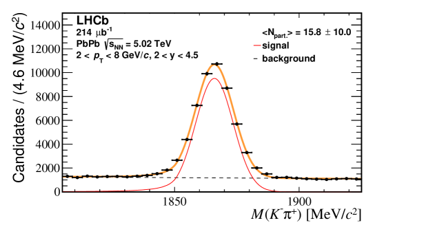
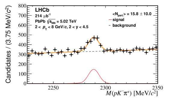
The signal extraction is performed after the selection criteria listed in Sec. 2 are applied. Figure 1 shows the (top) ${{K}^{-}}{{\pi}^{+}}$ and (bottom) $p{{K}^{-}}{{\pi}^{+}}$ invariant-mass spectra for the selected ${D}^{0}$ and ${\mathchar 28931\relax}^{+}_{c}$ candidates, respectively. The data are fitted using unbinned maximum-likelihood fits combining a Crystal Ball (CB) function [45] for the signal, and a first-order polynomial function for the background. While the CB function is chosen as it models the radiative tail of the invariant mass peak, the first-order polynomial function is chosen empirically to describe the observed background. The mean and width of the CB function are left free, while other parameters are fixed with those from simulation. An alternative used to assess systematic uncertainty for the background description is to multiply the first-order polynomial by an exponential function. The total number of fitted ${D}^{0}$ (${\mathchar 28931\relax}^{+}_{c}$) signal yield is $46000$ ($600$) events.

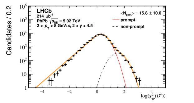
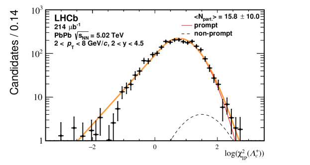
To discriminate prompt ${D}^{0}$ (${\mathchar 28931\relax}^{+}_{c}$) from those from a ${b}$-hadron decay, the background contribution is first subtracted from the datasets using the sPlot technique [46]. A fit to the $\log(\chi^{2}_{\text{IP}})$ distribution is performed to discriminate the prompt from non-prompt contributions. The $\chi^{2}_{\text{IP}}$ is defined as the difference in the vertex-fit $\chi^{2}$ of a given PV reconstructed with and without the candidate under consideration. An example of such fit is given in Fig. 2, where the $\log(\chi^{2}_{\text{IP}})$ distributions are fitted with a CB (Gaussian) function for the prompt (non-prompt) component.

Figure 1: Invariant-mass spectra of (top) ${{K}^{-}}{{\pi}^{+}}$ and (bottom) $p{{K}^{-}}{{\pi}^{+}}$ final states. The data are overlaid with the results of the fit.

Figure 2: Distributions of $\chi^{2}_{\text{IP}}$ of the ${D}^{0}$ (top) and ${\mathchar 28931\relax}^{+}_{c}$ (bottom) after background substraction. The data are overlaid with the results of the fit.

3.3 Efficiency estimation

The total efficiency ($\epsilon_{\rm tot}$) is factorized as

$$\epsilon_{\rm tot}^{{{D}^{0}},{{\mathchar 28931\relax}^{+}_{c}}}(p_{\mathrm{T}},y\ {\rm or}\ N_{c})=\epsilon_{\mathrm{acc}}^{{{D}^{0}},{{\mathchar 28931\relax}^{+}_{c}}}(p_{\mathrm{T}},y)\times\epsilon_{\mathrm{rec\&sel}}^{{{D}^{0}},{{\mathchar 28931\relax}^{+}_{c}}}(p_{\mathrm{T}},y\ {\rm or\ }N_{c})\times\epsilon_{\mathrm{PID}}^{{{D}^{0}},{{\mathchar 28931\relax}^{+}_{c}}}(p_{\mathrm{T}},y\ {\rm or\ }N_{c}),$$ (3)

where $\epsilon_{\mathrm{acc}}$ is the acceptance efficiency; $\epsilon_{\mathrm{rec\&sel}}$ is the reconstruction and selection efficiency; $\epsilon_{\mathrm{PID}}$ is the PID selection efficiency; $(N_{c},p_{\mathrm{T}},y)$ indicate given ranges in $N_{c}$, $p_{\mathrm{T}}$ and rapidity.

The acceptance efficiency $\epsilon_{\mathrm{acc}}$, for both ${\mathchar 28931\relax}^{+}_{c}$ and ${D}^{0}$ hadrons, is defined as

$$\epsilon_{\mathrm{acc}}^{{{D}^{0}},{{\mathchar 28931\relax}^{+}_{c}}}(p_{\mathrm{T}},y)=\frac{N_{\rm cand}^{2<y<4.5}}{N_{\rm cand}^{\rm fid}},$$ (4)

where $N_{\rm cand}^{\rm fid}$ are simulated ${D}^{0}$ or ${\mathchar 28931\relax}^{+}_{c}$ yields within the fiducial acceptance and $N_{\rm cand}^{2<y<4.5}$ indicate the number of the candidates with their decay products’ rapidity within $2<y<4.5$. The fiducial acceptance is defined as $2<y<4.5$ and $2<p_{\mathrm{T}}<8$$\text{\,Ge\kern-1.00006ptV\!/}c$. This efficiency is directly computed from simulation based on PYTHIA 8.

The reconstruction and selection efficiency $\epsilon_{\mathrm{rec\&sel}}$, for both ${\mathchar 28931\relax}^{+}_{c}$ and ${D}^{0}$ particles, is defined as:

$$\epsilon_{\mathrm{rec\&sel}}^{{{D}^{0}},{{\mathchar 28931\relax}^{+}_{c}}}(p_{\mathrm{T}},y\ \rm{or}\ N_{c})=\frac{N_{\rm cand}^{\rm rec.\&sel.}}{N_{\rm cand}^{2<y<4.5}},$$ (5)

where $N_{\rm cand}^{\rm rec.\&sel.}$ are reconstructed ${D}^{0}$ and ${\mathchar 28931\relax}^{+}_{c}$ candidates passing the selection criteria within the simulation samples. Several sources of bias are considered for $\epsilon_{\mathrm{rec\&sel}}$. The first source is the tracking algorithm efficiency, defined as the efficiency to reconstruct a track. Rather than directly measuring the tracking efficiency, the ratio of the efficiency between data and simulation is estimated using two $D^{0}$ calibration channels ($D^{0}\rightarrow K^{-}\pi^{+}$ and $D^{0}\rightarrow K^{-}\pi^{+}\pi^{-}\pi^{+}$). Their yields are evaluated in $\mathrm{Pb}\mathrm{Pb}$ data and simulation and the difference of their ratio from unity is encoded in a factor $k$. Results are given in Table 2. Other sources of systematic uncertainty are the ab-initio assumptions on the $p_{\mathrm{T}}$, $y$ and $N_{c}$ distributions, and correlation effects between these variables not accounted for with the embedding technique. To account for all these effects, an iterative method based on data is employed. In the first step, the raw (i.e not corrected for inefficiency) $p_{\mathrm{T}}$, rapidity, and $N_{c}$ distributions are extracted from the data based on the signal extraction defined in Sec. 3.2. In the second step, these distributions are corrected using the data-to-simulation tracking efficiency ($k$ factor) and the PID efficiency ($\epsilon_{\mathrm{PID}}$) computed with the raw kinematic distributions reconstructed in the simulation. In the third step, the reconstructed distributions from the simulation are weighted using several iterations until they match the data as a function of $p_{\mathrm{T}}$, $y$, and $N_{c}$ simultaneously. Finally, $\epsilon_{\mathrm{rec\&sel}}$ is computed in step four. Steps two to four are repeated until $\epsilon_{\mathrm{rec\&sel}}$ converges to a final value, which is the case after three iterations.

Table 2: Value of the $k$ factor in intervals of $N_{c}$. The uncertainties are obtained from the statistical uncertainties of the different ${D}^{0}$ calibration samples in data and MC summed in quadrature.

$N_{c}$ interval		$k(N_{c})$
1000 –	4000	0.97$\pm$	0.03
4000 –	5500	0.93$\pm$	0.04
5500 –	10000	0.91$\pm$	0.05

The PID efficiency $\epsilon_{\mathrm{PID}}$ is computed using the weighted simulation samples. The methodology is similar to that used for $p$ $p$ collisions [47], and is based on a tag-and-probe technique. In this approach, the $\epsilon_{\mathrm{PID}}$ for a given probe particle $\epsilon_{\mathrm{PID}}^{\rm part}$ (e.g. pion) is computed from a reference sample (e.g. ${{D}^{0}}\rightarrow{{K}^{-}}{{\pi}^{+}}$) where a tight selection cut on the tag particle (i.e. the kaon) is applied, while no PID selection is applied to the probe particle. In the next step, the sPlot technique [46] is used to remove the background with the invariant mass as a discriminating variable. Finally, the PID efficiency of the probe is computed as the fraction of candidates (i.e. ${D}^{0}$) fulfilling given PID requirement.

Kaon and pion PID efficiencies are computed using the $\mathrm{Pb}\mathrm{Pb}$ ${D}^{0}$ sample, while the proton efficiency is computed from ${\mathchar 28931\relax}\rightarrow{{\pi}^{-}}p$ decays in $\mathrm{Pb}\mathrm{Pb}$ data. Two-dimensional maps are then computed for each particle (i.e kaon, pion, proton) as a function of $p$ and $y$, for different ranges in $N_{c}$. Finally, these maps are used to compute hadron PID efficiency for ${D}^{0}$ and ${\mathchar 28931\relax}^{+}_{c}$ candidates as

$$\epsilon_{\mathrm{PID}}^{{{D}^{0}},{{\mathchar 28931\relax}^{+}_{c}}}(p_{\mathrm{T}},y\ {\rm or}\ N_{c})=\frac{\prod^{\rm candidate}_{\rm part}\epsilon_{\mathrm{PID}}^{\rm part}(p,y,N_{c})}{N_{\rm cand}^{\rm rec.\&sel.}},$$ (6)

where $\epsilon_{\mathrm{PID}}^{\rm part}(p,y,N_{c})$ is the single-particle efficiency.

4 Systematic uncertainties

Several sources of systematic uncertainty on $R_{{{\mathchar 28931\relax}^{+}_{c}}/{{D}^{0}}}$ are considered. For the signal extraction, three parametrizations of the CB functions with different values of $\alpha$ are combined with the two background shapes. The systematic uncertainties are taken as the RMS of the results of all the fits for a given bin, considered as uncorrelated between the kinematic intervals. A similar strategy is employed for the prompt fraction estimation, where the Gaussian function is replaced by a Bukin function [48].

Four sources of systematic uncertainty are considered for the iterative method used to compute $\epsilon_{\mathrm{rec\&sel}}$ and $\epsilon_{\mathrm{PID}}$: (i) the uncertainty on the $k$ factor; (ii) the choice of the binning used for the reference raw data distribution; (iii) the sensitivity to the initial reference data distribution; (iv) the uncertainty on the PID maps. For each source, $\epsilon_{\mathrm{rec\&sel}}$ and $\epsilon_{\mathrm{PID}}$ are computed, and the RMS of all the variations are taken as the systematic uncertainties. For the first source, new results have been obtained on $R_{{{\mathchar 28931\relax}^{+}_{c}}/{{D}^{0}}}$ using 20 values of $k$, varied within uncertainties. The systematic uncertainty associated with the choice of the binning scheme is evaluated by using a finer scheme than the nominal one. The sensitivity to the initial reference distributions is tested by evaluating them using an sPlot technique instead of a fit of invariant-mass spectra. Finally, the uncertainty linked to the PID maps is evaluated using a smearing technique to compute 20 PID maps where an efficiency in each bin is randomly varied within its statistical uncertainty.

All the systematic uncertainties are summarized in Table 3. Each uncertainty category is treated as uncorrelated and is added in quadrature. Systematic uncertainty arising from the $\mathcal{B}$ ratio of ${{D}^{0}}\rightarrow{{K}^{-}}{{\pi}^{+}}$ and ${{\mathchar 28931\relax}^{+}_{c}}\rightarrow p{{K}^{+}}{{\pi}^{-}}$ decays, entering Eq.1, is also included in Table 3. This contribution is fully correlated between different kinematic variable intervals.

Table 3: Summary of the ranges of systematic uncertainties for the considered intervals of $N_{c}$, $p_{\mathrm{T}}$ and $y$ for the $R_{{{\mathchar 28931\relax}^{+}_{c}}/{{D}^{0}}}$ ratio given in percentage.

Source $N_{c}$ $p_{\mathrm{T}}$ ($\text{\,Ge\kern-1.00006ptV\!/}c$) $y$ $\epsilon_{\rm tot}$ (stat.) 5.1–7.1 4.1–5.1 4.1–7.1 Invariant-mass fit 1–5 1–5 1–5 $f_{\rm prompt}$ 1.8–8.1 1.4–10.2 3.4–4.6 $\epsilon_{\rm acc}$ $<$1 $<$1 $<$1 $k$ factor 1.8–3.8 1.6–2.1 1.6–1.8 Iterative procedure 7–9 4–11 4–8 Total 9–12 8–14 8–10 Ratio of branching fractions 5.16 5.16 5.16

5 Results

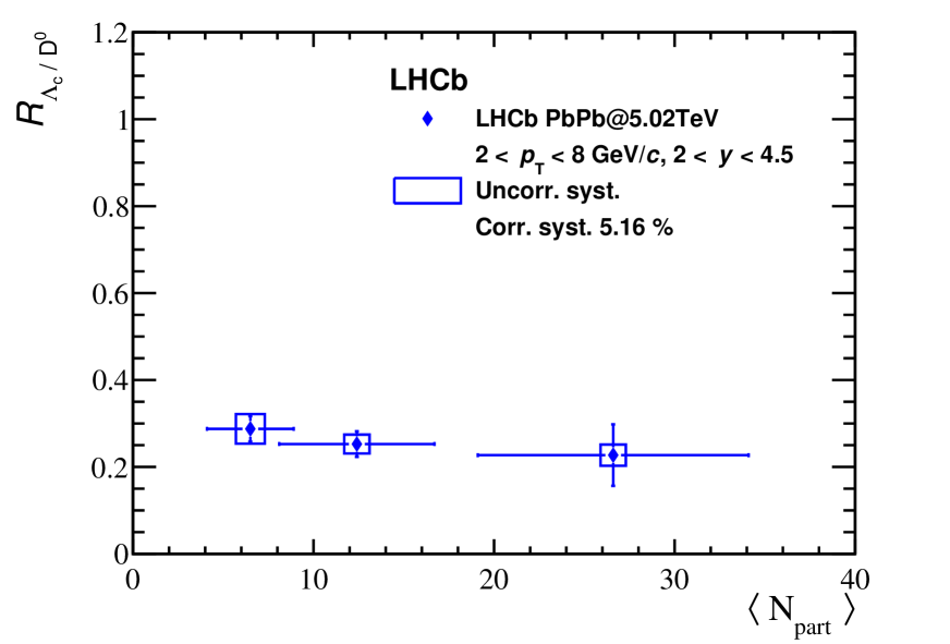
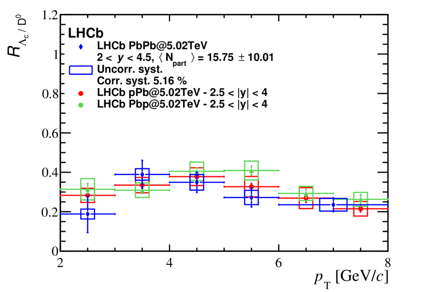
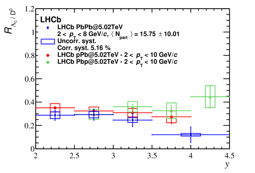
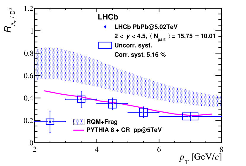
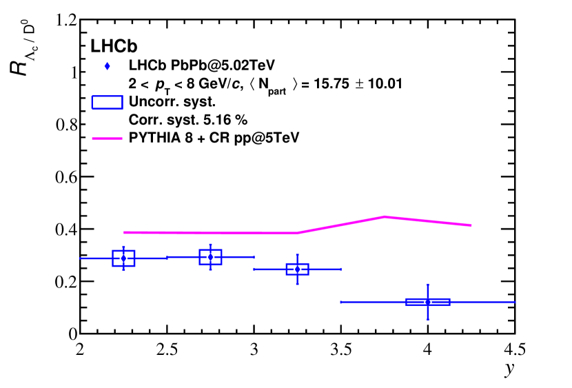
Results for the $R_{{{\mathchar 28931\relax}^{+}_{c}}/{{D}^{0}}}$ production ratio are given in Table 4. The $N_{c}$ variable is replaced by $\langle\mathrm{N_{part}}\rangle$ as shown in Table 1. As can be seen in Fig. 3, $R_{{{\mathchar 28931\relax}^{+}_{c}}/{{D}^{0}}}$ shows no dependence on $\langle\mathrm{N_{part}}\rangle$, within uncertainties, with a mean value $\langle R_{{{\mathchar 28931\relax}^{+}_{c}}/{{D}^{0}}}\rangle\sim 0.27$. In Fig. 4, the $p_{\mathrm{T}}$ and $y$ dependent $R_{{{\mathchar 28931\relax}^{+}_{c}}/{{D}^{0}}}$ results are compared to those from ${p}\mathrm{Pb}$ data at $\sqrt{s_{\scriptscriptstyle\text{NN}}}=5.02\text{\,Te\kern-1.00006ptV}$ [22], showing a good agreement between the measurements. This observation is consistent with the fact that the two samples have relatively close center-of-mass energy, and similar $\langle\mathrm{N_{part}}\rangle$ values. The same measurements of $R_{{{\mathchar 28931\relax}^{+}_{c}}/{{D}^{0}}}$ versus $p_{\mathrm{T}}$ and $y$ are compared to theoretical predictions in Fig. 5. Both dependencies are compared to predictions from PYTHIA 8 [15] in $p$ $p$ collisions at $\sqrt{s}$ = 5.02  TeV. For these predictions, a special tuning is used to increase the ${\mathchar 28931\relax}^{+}_{c}$ coalescence from charm production at the expense of $D$ mesons. In addition, the CR mechanism is also allowed. A good description of the $p_{\mathrm{T}}$ trend is found between theory and data for $p_{\mathrm{T}}>5\text{\,Ge\kern-1.00006ptV\!/}c$, while tensions are observed at low $p_{\mathrm{T}}$. The constant trend versus rapidity is reproduced by theory predictions within three standard deviations, except for the most forward region likely due to a fluctuation in the data. The $p_{\mathrm{T}}$ dependence is also compared to predictions from the SHM [20] for which an augmented set of excited charm-baryon states decaying into ${\mathchar 28931\relax}^{+}_{c}$ is added to the fragmentation mechanism. According to this model, these additional states could explain the large $R_{{{\mathchar 28931\relax}^{+}_{c}}/{{D}^{0}}}$ observed by the ALICE experiment. These predictions are systematically higher than the LHCb data versus $p_{\mathrm{T}}$.

Table 4: Results for the prompt $R_{{{\mathchar 28931\relax}^{+}_{c}}/{{D}^{0}}}$ production ratio, where the first uncertainties are statistical and the second systematic. A fully correlated systematic uncertainty of 5.16%, due to the limited knowledge of the external branching fractions, affects all the intervals.

$p_{\mathrm{T}}$ (GeV/$c$) $R_{{{\mathchar 28931\relax}^{+}_{c}}/{{D}^{0}}}$  2 – 3 0.188 $\pm$ 0.095 $\pm$ 0.025  3 – 4 0.389 $\pm$ 0.072 $\pm$ 0.029  4 – 5 0.349 $\pm$ 0.052 $\pm$ 0.040  5 – 6 0.272 $\pm$ 0.049 $\pm$ 0.036  6 – 8 0.235 $\pm$ 0.035 $\pm$ 0.032 $y$ $R_{{{\mathchar 28931\relax}^{+}_{c}}/{{D}^{0}}}$  2.0 – 2.5 0.288 $\pm$ 0.044 $\pm$ 0.029  2.5 – 3.0 0.292 $\pm$ 0.048 $\pm$ 0.028  3.0 – 3.5 0.246 $\pm$ 0.056 $\pm$ 0.020  3.5 – 4.5 0.120 $\pm$ 0.067 $\pm$ 0.011 $\langle\mathrm{N_{part}}\rangle$ $\pm$ $\sigma_{\rm part}$ $R_{{{\mathchar 28931\relax}^{+}_{c}}/{{D}^{0}}}$  6.5 $\pm\ 2.5$ 0.288 $\pm$ 0.029 $\pm$ 0.034 12.4 $\pm\ 4.4$ 0.253 $\pm$ 0.029 $\pm$ 0.022 26.6 $\pm\ 7.5$ 0.227 $\pm$ 0.071 $\pm$ 0.024

Figure 3: Prompt $R_{{{\mathchar 28931\relax}^{+}_{c}}/{{D}^{0}}}$ production ratios as a function of $\langle\mathrm{N_{part}}\rangle$. The error bars along the y-axis (x-axis) represent the statistical uncertainties (RMS of the $\langle\mathrm{N_{part}}\rangle$ value), the boxes around the points the uncorrelated systematic uncertainties.

Figure 4: Prompt $R_{{{\mathchar 28931\relax}^{+}_{c}}/{{D}^{0}}}$ production ratios as a function of (left) $p_{\mathrm{T}}$ and (right) rapidity. The error bars represent the statistical uncertainties, the boxes around the points the uncorrelated systematic uncertainties. Results are compared to the same measurement in ${p}\mathrm{Pb}$ and $\mathrm{Pb}{p}$ collisions at $\sqrt{s_{\scriptscriptstyle\text{NN}}}$ = 5.02 TeV by the LHCb experiment [33].

Figure 5: Prompt $R_{{{\mathchar 28931\relax}^{+}_{c}}/{{D}^{0}}}$ production ratios as a function of (left) $p_{\mathrm{T}}$ and (right) rapidity. The error bars represent the statistical uncertainties, the boxes around the points the uncorrelated systematic uncertainties. Results are compared to PYTHIA 8 [15] in $p$ $p$ collisions at $\sqrt{s}$ = 13 TeV (magenta band) and predictions from a Statical Hadronization Model [20] (blue band).

6 Conclusions

This paper reports the first measurements of the $R_{{{\mathchar 28931\relax}^{+}_{c}}/{{D}^{0}}}$ production cross-section ratio in peripheral $\mathrm{Pb}\mathrm{Pb}$ collisions at $\sqrt{s_{\scriptscriptstyle\text{NN}}}$ = 5.02  TeV by the LHCb experiment. The $R_{{{\mathchar 28931\relax}^{+}_{c}}/{{D}^{0}}}$ shows no significant dependence on either rapidity or $\langle\mathrm{N_{part}}\rangle$ within uncertainties, and has a mean value of $\langle R_{{{\mathchar 28931\relax}^{+}_{c}}/{{D}^{0}}}\rangle\sim 0.27$. However, the ratio tends to decrease at lower $p_{\mathrm{T}}$. More data are needed to confirm the results. Results are consistent with previous LHCb measurements in ${p}\mathrm{Pb}$ collisions at $\sqrt{s_{\scriptscriptstyle\text{NN}}}$ = 5.02  TeV [33]. Compared to theory predictions, the results are compatible within one standard deviation with the PYTHIA 8 predictions in $p$ $p$ collisions at $\sqrt{s}$ = 5.02  TeV, including the CR mechanism, except at low $p_{\mathrm{T}}$. In contrast, a systematic discrepancy versus $p_{\mathrm{T}}$ is observed with the SHM model predictions. These new experimental results point toward a strong dependence of $R_{{{\mathchar 28931\relax}^{+}_{c}}/{{D}^{0}}}$ with rapidity, which helps to constrain theory predictions in this particular phase-space region.

References

- [1] P. Braun-Munzinger, V. Koch, T. Schäfer, and J. Stachel, Properties of hot and dense matter from relativistic heavy ion collisions, Phys. Rept. 621 (2016) 76, arXiv:1510.00442
- [2] HotQCD collaboration, A. Bazavov et al., Equation of state in (2+1)-flavor QCD, Phys. Rev. D90 (2014) 094503, arXiv:1407.6387
- [3] P. B. Gossiaux, Open heavy flavours in nuclear collisions: Theory overview, Nucl. Phys. A982 (2019) 113, arXiv:1901.01606
- [4] A. Andronic et al., Heavy-flavour and quarkonium production in the LHC era: from proton–proton to heavy-ion collisions, Eur. Phys. J. C76 (2016) 107, arXiv:1506.03981
- [5] F. Prino and R. Rapp, Open heavy flavor in QCD matter and in nuclear collisions, J. Phys. G43 (2016) 093002, arXiv:1603.00529
- [6] CLEO collaboration, M. Artuso et al., Charm meson spectra in annihilation at 10.5 GeV center of mass energy, Phys. Rev D70 (2004) 112001, arXiv:hep-ex/0402040
- [7] Belle collaboration, R. Seuster et al., Charm hadrons from fragmentation and B decays in annihilation at , Phys. Rev. D73 (2006) 032002, arXiv:hep-ex/0506068
- [8] BaBar collaboration, B. Aubert et al., Measurement of and production in meson decays and from continuum annihilation at GeV, Phys. Rev. D65 (2002) 091104, arXiv:hep-ex/0201041
- [9] LHCb collaboration, R. Aaij et al., Prompt charm production in collisions at 7 TeV, Nucl. Phys. B871 (2013) 1, arXiv:1302.2864
- [10] LHCb collaboration, R. Aaij et al., Measurements of prompt charm production cross-sections in collisions at 13 TeV, JHEP 03 (2016) 159, Erratum ibid. 09 (2016) 013, Erratum ibid. 05 (2017) 074, arXiv:1510.01707
- [11] LHCb collaboration, R. Aaij et al., Measurements of prompt charm production cross-sections in collisions at 5 TeV, JHEP 06 (2017) 147, arXiv:1610.02230
- [12] ALICE collaboration, S. Acharya et al., production in pp collisions at TeV and in p-Pb collisions at TeV, JHEP 04 (2018) 108, arXiv:1712.09581
- [13] ALICE collaboration, S. Acharya et al., production in Pb-Pb collisions at TeV, Phys. Lett. B793 (2019) 212, arXiv:1809.10922
- [14] ALICE collaboration, S. Acharya et al., production in and in -Pb collisions at =5.02 TeV, Phys. Rev. C104 (2021) 054905, arXiv:2011.06079
- [15] J. R. Christiansen and P. Z. Skands, String formation beyond leading colour, JHEP 08 (2015) 003, arXiv:1505.01681
- [16] S. Plumari et al., Charmed hadrons from coalescence plus fragmentation in relativistic nucleus-nucleus collisions at RHIC and LHC, Eur. Phys. J. C78 (2018) 348, arXiv:1712.00730
- [17] CMS collaboration, A. M. Sirunyan et al., Production of baryons in proton-proton and lead-lead collisions at 5.02 TeV, Phys. Lett. B803 (2020) 135328, arXiv:1906.03322
- [18] STAR collaboration, J. Adam et al., First measurement of baryon production in Au+Au collisions at = 200 GeV, Phys. Rev. Lett. 124 (2020) 172301, arXiv:1910.14628
- [19] Y. Oh, C. M. Ko, S. H. Lee, and S. Yasui, Heavy baryon/meson ratios in relativistic heavy ion collisions, Phys. Rev. C79 (2009) 044905, arXiv:0901.1382
- [20] M. He and R. Rapp, Hadronization and charm-hadron ratios in heavy-ion collisions, Phys. Rev. Lett. 124 (2020) 042301, arXiv:1905.09216
- [21] M. He and R. Rapp, Charm-baryon production in proton-proton collisions, Phys. Lett. B795 (2019) 117, arXiv:1902.08889
- [22] LHCb collaboration, R. Aaij et al., Prompt production in collisions at TeV, JHEP 02 (2019) 102, arXiv:1809.01404
- [23] K. J. Eskola, H. Paukkunen, and C. A. Salgado, EPS09: A new generation of NLO and LO nuclear parton distribution functions, JHEP 04 (2009) 065, arXiv:0902.4154
- [24] K. Kovarik et al., nCTEQ15 - Global analysis of nuclear parton distributions with uncertainties in the CTEQ framework, Phys. Rev. D93 (2016) 085037, arXiv:1509.00792
- [25] LHCb collaboration, A. A. Alves Jr. et al., The LHCb detector at the LHC, JINST 3 (2008) S08005
- [26] LHCb collaboration, R. Aaij et al., LHCb detector performance, Int. J. Mod. Phys. A30 (2015) 1530022, arXiv:1412.6352
- [27] R. Aaij et al., Performance of the LHCb Vertex Locator, JINST 9 (2014) P09007, arXiv:1405.7808
- [28] P. d’Argent et al., Improved performance of the LHCb Outer Tracker in LHC Run 2, JINST 12 (2017) P11016, arXiv:1708.00819
- [29] M. Adinolfi et al., Performance of the LHCb RICH detector at the LHC, Eur. Phys. J. C73 (2013) 2431, arXiv:1211.6759
- [30] A. A. Alves Jr. et al., Performance of the LHCb muon system, JINST 8 (2013) P02022, arXiv:1211.1346
- [31] R. Aaij et al., The LHCb trigger and its performance in 2011, JINST 8 (2013) P04022, arXiv:1211.3055
- [32] LHCb collaboration, R. Aaij et al., Precision luminosity measurements at LHCb, JINST 9 (2014) P12005, arXiv:1410.0149
- [33] LHCb collaboration, R. Aaij et al., Prompt production in Pb collisions at TeV, JHEP 02 (2019) 102, arXiv:1809.01404
- [34] T. Sjostrand, S. Mrenna, and P. Z. Skands, A brief introduction to PYTHIA 8.1, Comput. Phys. Commun. 178 (2008) 852, arXiv:0710.3820
- [35] S. Porteboeuf, T. Pierog, and K. Werner, Producing hard processes regarding the complete event: the EPOS event generator, 45th Rencontres de Moriond on QCD and High Energy Interactions (2010) 135, arXiv:1006.2967
- [36] T. Pierog et al., EPOS LHC: Test of collective hadronization with data measured at the CERN large hadron collider, Phys. Rev. C92 (2015) 034906, arXiv:1306.0121
- [37] D. J. Lange, The EvtGen particle decay simulation package, Nucl. Instrum. Meth. A462 (2001) 152
- [38] P. Golonka and Z. Was, PHOTOS Monte Carlo: A precision tool for QED corrections in and decays, Eur. Phys. J. C45 (2006) 97, arXiv:hep-ph/0506026
- [39] Geant4 collaboration, S. Agostinelli et al., Geant4: A simulation toolkit, Nucl. Instrum. Meth. A506 (2003) 250
- [40] Geant4 collaboration, J. Allison et al., Geant4 developments and applications, IEEE Trans. Nucl. Sci. 53 (2006) 270
- [41] M. Clemencic et al., The LHCb simulation application, Gauss: Design, evolution and experience, J. Phys. Conf. Ser. 331 (2011) 032023
- [42] Particle Data Group, P. A. Zyla et al., Review of particle physics, Prog. Theor. Exp. Phys. 2020 (2020) 083C01
- [43] C. Loizides, J. Nagle, and P. Steinberg, Improved version of the PHOBOS Glauber monte carlo, doi: 10.1016/j.softx.2015.05.001 arXiv:1408.2549
- [44] LHCb collaboration, R. Aaij et al., Centrality determination in heavy-ion collisions with the LHCb detector, arXiv:2111.01607
- [45] T. Skwarnicki, A study of the radiative cascade transitions between the Upsilon-prime and Upsilon resonances, PhD thesis, Institute of Nuclear Physics, Krakow, 1986, DESY-F31-86-02
- [46] M. Pivk and F. R. Le Diberder, sPlot: A statistical tool to unfold data distributions, Nucl. Instrum. Meth. A555 (2005) 356, arXiv:physics/0402083
- [47] L. Anderlini et al., The PIDCalib package, LHCb-PUB-2016-021, 2016
- [48] A. D. Bukin, Fitting function for asymmetric peaks, arXiv:0711.4449