Prediction can be safely used as a proxy for explanation in causally consistent Bayesian generalized linear models

Abstract

Bayesian modeling provides a principled approach to quantifying uncertainty in model parameters and model structure and has seen a surge of applications in recent years. Within the context of a Bayesian workflow, we are concerned with model selection for the purpose of finding models that best explain the data, that is, help us understand the underlying data generating process. Since we rarely have access to the true process, all we are left with during real-world analyses is incomplete causal knowledge from sources outside of the current data and model predictions of said data. This leads to the important question of when the use of prediction as a proxy for explanation for the purpose of model selection is valid. We approach this question by means of large-scale simulations of Bayesian generalized linear models where we investigate various causal and statistical misspecifications. Our results indicate that the use of prediction as proxy for explanation is valid and safe only when the models under consideration are sufficiently consistent with the underlying causal structure of the true data generating process.

Keywords Bayesian workflow  $\cdot$ causal inference  $\cdot$ explanation  $\cdot$ prediction  $\cdot$ generalized linear models  $\cdot$ simulation study

1 Introduction

Probabilistic modeling provides a principled approach to quantifying uncertainty in model parameters and model structure. In recent years, it has seen a surge of applications in almost all quantitative sciences and industrial areas (Gelman et al., 2013; McElreath, 2020; Gelman et al., 2020a). To support the principled application of Bayesian methods, Gelman et al. (2020a) proposed an overarching workflow to conduct Bayesian data analysis. In short, the workflow asks users to pick an initial model and iteratively refine it, performing various checks on the way to ensure that probabilistic assumptions are sensible, computations are valid, and model results are trustworthy for the intended purposes. This basic model building loop is repeated until either the user’s requirements are satisfied or no satisfactory model can be found with the available resources. Within this overarching workflow, there are still many unknowns when it comes to making optimal decisions for each iterative step or sub-workflow.

The current work is concerned with the decision-making process during model building iterations, namely model selection for the purpose of finding models that best explain the data, that is, help us understand the underlying data generating process. Unfortunately, explanation is an illusive concept in practice as, for real data, we have no direct access to the underlying data generating process. Thus, all we are left with during real-world analyses is incomplete causal knowledge from sources outside of the current data and model predictions of said data. The distinction between explanation (of the underlying process) and prediction (of observable data) has a long history in many fields of sciences engaged in model-based reasoning and inference (see Section 1.1). However, the statistical relationship of explanation and prediction is still not sufficiently understood, which is surprising given the importance of these concepts to statistical theory and practice.

To this end, we study the validity of using prediction as a proxy for explanation in Bayesian statistical models (see Figure 1 for a conceptual overview to be detailed later on). Our main conclusion can be summarized as follows: Using prediction as a proxy for explanation is valid and safe only when the considered models are sufficiently consistent with the underlying causal structure of the true data generating process. Specifically, our contributions are:

1. a conceptual introduction and overview of the relationship of explanation and prediction as well as their connection to causality;

2. large-scale simulations of Bayesian generalized-linear models to study said relationship under various causal and statistical misspecifications;

3. initial evidence that causality is indeed the missing link that connects prediction and explanation when comparing statistical models; and

4. a set of R packages (Scholz and Bürkner, 2022a; Scholz et al., 2022; Scholz and Bürkner, 2022b) that facilitate simulation studies of Bayesian models.

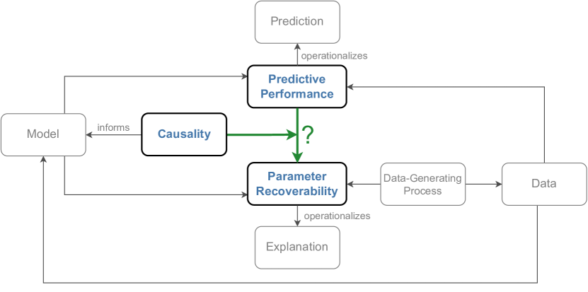
Figure 1: High-level overview of our conceptual framework that connects explanation and prediction in statistical modeling. See Section 1.1 for further details.

1.1 Explanation vs. Prediction

Douglas (2009) provides a historical overview of the relationship of prediction and explanation from the perspective of philosophy of science. She concludes that ’explanations are the means that help us think our way through to the next testable prediction’ (Douglas, 2009, page 462, Section 6). In other words, and more statistically speaking, explanations help us understand the inner workings of a process by means of a model, while prediction concerns the comparison of the model’s output to real-world observables. Explanation and prediction are not statistical concepts themselves, though. Instead, we have to operationalize them in terms of mathematical quantities computable from a statistical model. Following Bürkner et al. (2022a), we call the statistical operationalization of explanation parameter recoverability and the operationalization of prediction predictive performance:

Parameter Recoverability (PR) refers to a model’s ability to recover the latent (i.e., not directly observable) parameters of an assumed true data-generating process (DGP), for example, the true effect size of a treatment for a medical condition (Bürkner et al., 2022a). This implies that assessing PR requires concrete knowledge of the true DGP including its true parameter values. Accordingly, it can only be studied directly in artificial settings where the true DGP is known, with the hope that the real data of interest fulfills the assumptions of these artificial settings sufficiently well.

Predictive Performance (PP) describes the ability of a model to accurately predict new observations from existing observations, for example, predicting a diagnosis based on symptoms and medical history (Hastie et al., 2009; Gabaix and Laibson, 2008). It is one of the most prominent utilities for gauging model performance in data analysis and a central tool for model comparisons (Vehtari and Ojanen, 2012; Gelman et al., 2013; Vehtari et al., 2017). In most cases, one is interested in out-of-sample PP, as predicting unseen data is almost always the primary goal of modeling (Vehtari and Ojanen, 2012). PP is conceptually similar to PR in that both target the accurate estimation of model-implied quantities (Bürkner et al., 2022a), with the main difference that the former targets quantities that are observable at real data inference time (i.e., outcome variables), which allows to derive estimates that are agnostic with respect to the true DGP (Vehtari and Ojanen, 2012).

In the following, we present some of the common perspectives on prediction and explanation as well as their connections with causality. When talking about these concepts from statistical perspectives, we use them and their operationalizations interchangeably.

1.1.1 Explanation only

The statistical field that is probably most interested in explanation in the form of unbiased estimators is that of causality (Pearl, 2009a). The do-calculus (Pearl, 2012) and equivalently the potential outcomes framework (Rubin, 1974, 1978) offer sound theories to identify models that are able to provide an unbiased estimate of a parameter of choice. We call a model ’causally consistent’ if it is consistent with a theoretically justified causal graph of its contributing variables (Bürkner et al., 2022a). This consistency is necessary for models to provide at least asymptotically unbiased estimates for latent parameters.

While the ability to find an unbiased estimator is highly valuable, it is not the only metric we need to pay attention to. As argued for example by Shmueli (2010), optimizing the overall bias-variance trade-off is a sensible alternative goal, which also requires to minimize the variance of a parameter estimator in addition to minimizing its bias. Examples in the causal literature that attempt to additionally reduce variance are the works of Henckel et al. (2022) and Rotnitzky and Smucler (2020), which use graphical criteria to find lower variance estimators (see also Cinelli et al., 2020, for a more general overview). However, we found that the reduction of variance is only considered after unbiasedness has been established. Thus, no actual bias-variance trade-off is allowed to take place from this perspective. Additionally, predictive performance considerations are missing altogether from the general discussion in the causal literature. We go into more details about how causal consistency serves as the foundation of the presented study in Section 2.1.

1.1.2 Explanation first

Arguably the most prominent perspective on the relationship of explanation and prediction is coming from the philosophy of science (as examplarily presented by Ramspek et al., 2021; Navarro, 2019; Hernán et al., 2019; Yarkoni and Westfall, 2017; Shmueli, 2010; Breiman, 2001) in cognitive-, social-, and life-sciences. The main discussion point is that, even if explanation is the main research goal, the value of good prediction shouldn’t simply be ignored. Yarkoni and Westfall (2017) and Breiman (2001) are examples for the call to put more focus on predictions, even if explanation is the main goal. The underlying argument is that a model with bad predictive performance has a higher chance of misrepresenting or missing relevant features of the true DGP. One should thus be careful when relying on the explanations of a model with weak predictive performance. Similarly, Shmueli (2010) makes the argument that predictive power cannot be inferred from explanatory power, that is, good explanatory models do not automatically lead to good predictions. A common proposal is to use a predictive model (i.e., a model that maximizes predictive performance) as a benchmark (Shmueli, 2010; Cranmer and Desmarais, 2017) to aim for with an explanatory model (i.e., a model that maximizes parameter recoverability). Douglas (2009) gives an illustrative example for this approach with the discovery of Pluto. The paths of Uranus and Neptune did not follow their predicted paths which implied a problem with the explanatory model. The solution was the discovery of Pluto, which explained the observed deviation and lead to an updated model. Finally, while there are sound high level arguments for why models that provide better explanations should generally provide better predictions as well, we are not aware of other works that investigate this relationship further besides common textbook examples of improved predictions despite bad parameter recovery in the face of causal misspecification (McElreath, 2020).

1.1.3 Prediction first

Machine-learning models are sometimes also called black box models due to the fact that they solely focus on providing the best possible predictions while their inner workings are hard or impossible to understand and do not directly map to any assumed DGP. The lack of interpretability, and thus potential to provide explanations, is a common critique of machine learning techniques, more recently more work has been done to improve this aspect (see for example Gilpin et al., 2018; Carvalho et al., 2019). While predictive performance remains the main goal of these models, requirements regarding responsible reporting and accountability as well as improved performance for small sample sizes led to the incorporation of causal assumptions, which are a requirement for reliable explanations (Li et al., 2022; Richens et al., 2020; Schölkopf, 2022). And while not necessarily using the same causal vocabulary, the idea of physics-informed neural networks (Raissi et al., 2019; Karniadakis et al., 2021) is closely related, as the partial or ordinary differential equations describing physical processes can be understood as causal constraints that have to be met.

However, with the increasing requirements for explainable AI (Arrieta et al., 2020) in fields like medicine, aspects such as feature importance (Lundberg and Lee, 2017; Ribeiro et al., 2016) become more relevant to understand how machine learning models make decisions. Such aspects can be seen as extending the concept of explanation in some sense, although this has not been explored systematically to our knowledge and, at least in the stricter sense of recovering (latent) parameters of an assumed DGP, explanation is not really a concern in machine learning in general.

1.1.4 Combining explanation, prediction, and causality

Based on the presented perspectives, there is an apparent gap in the joint consideration of explanation, prediction, and causality. In this paper, we approach this joint consideration from the perspective of model selection in a Bayesian workflow (see Figure 1 for an illustration). When explanation is the goal, prediction reduces to a conveniently available supporting utility that ideally helps to select better explaining models at real data inference time (Bürkner et al., 2022a). In practice at least, and despite the theoretical arguments for caution, this assumption is very commonly (and often implicitly) made whenever explanatory model choices are based on out-of-sample posterior predictive metrics or their approximations, such as AIC (e.g., Watanabe, 2009; McElreath, 2020), DIC (Spiegelhalter et al., 1998), WAIC (Watanabe and Opper, 2010; Vehtari et al., 2017) or ELPD-LOO (Vehtari and Ojanen, 2012; Vehtari et al., 2017). As we know from counterexamples (Betancourt, 2020; Hagerty and Srinivasan, 1991), this assumption cannot hold in general, but it remains unclear under which conditions it is actually justified. The goal of this paper is to investigate under which circumstances this proxy use might be valid.

1.2 Generalized Linear Models

We focus our studies on the class of Bayesian generalized linear models (GLMs). This choice is motivated by the fact that they represent the minimal general class of models that enable us to investigate the utility of using prediction as a proxy for explanation. GLMs allow us to represent causal DAGs while adding the ability to change model aspects that are not DAG-dependent (i.e., the likelihood family and link function). Despite (or perhaps because of) their simplicity, GLMs make up a big part of all statistical data analyses. Their success can be explained by several factors, involving the ease of interpretation of their additive structure, rich mathematical theory, and (relatively) straightforward estimation (Gelman et al., 2020b; Harrell, 2015; Nelder and Wedderburn, 1972; Gill et al., 2001).

More specifically, we consider GLMs of the form $y\sim\textrm{likelihood}(\textrm{link}^{-1}(\mu),\phi)$ with a univariate response variable $y$ that is assumed to follow a parametric likelihood distribution, often called a likelihood family (Bates et al., 2015; Bürkner, 2017), one main location parameter $\mu=\alpha+X\beta$ that is predicted, as well as zero or more auxiliary distributional parameters $\phi$ that are assumed to be constant over observations (Nelder and Wedderburn, 1972; Gill et al., 2001).

When setting up GLMs, the four important choices the analyst has to make are (i) the likelihood family, (ii) the link function, (iii) the linear predictor term, and (iv) whether and how to regularize, that is, for Bayesian GLMs, what prior distributions to use. All of these choices are mutually related (Gelman et al., 2017), but specifically (i) and (ii) are closely intertwined, as the choice of link function depends on the support of $\mu$ and thus on the chosen likelihood. We discuss our specific choices of likelihoods and link functions in Section 2.2, the specific models we generate data from in Section 2.3 and the models we fit on the generated data in Section 2.4.

1.3 Aims and Scope

As laid out in Section 1.1, there is a gap in the literature regarding the relationship of (the statistical operationalizations of) prediction and explanation under varying causal assumptions. The aim of this paper is not to fill said gap entirely but rather to be a starting point for further research. As explained above, direct measures of explanation are rarely accessible during real-world modeling and prediction provides a convenient (i.e., easily available) alternative for model selection. Even though the validity of the practice has so far remained unclear, prediction is commonly used as a proxy for explanation during practical model selection in the context of Bayesian or other statistical workflows. It is the main aim of this paper to empirically investigate the use of prediction as a proxy for explanation under several causal and statistical misspecification mechanisms in Bayesian GLMs. Further, the methods introduced in this paper could serve as a basis for further work, some of which we propose in Section 4.

While this paper focuses on Bayesian models, we assume that the presented results also hold for their frequentist counterparts, as the mechanisms of causality are agnostic to the specific method of estimation (under reasonable equivalence of estimators; see also Section 2.4).

2 Methods

As explained in Section 1.1, studying parameter recoverability (PR; the statistical operationalization of explanation) requires knowledge of the true data-generating process (DGP). Combined with the fact that we aim to study Bayesian GLMs, this renders an analytical approach infeasible and we thus resort to extensive simulations as the method of choice.

In this section, we start with an explanation of the causal foundation of the simulations and how we used it throughout the process in Section 2.1. We also provide an overview of the considered likelihood families and link functions in Section 2.2. Next, we walk through the study’s design (see Figure 2 for a conceptual overview), with data generation described in Section 2.3, model fitting in Section 2.4, and metric calculation in Section 2.5. Finally, we discuss the statistical analysis of the results of the simulations in Section 2.6.

Many aspects of this study are not only dependent on the methods and algorithms used, but also on their software implementations. The simulation was implemented in R (R Core Team, 2018) using Stan (Stan Development Team, 2022; Carpenter et al., 2017) and brms (Bürkner, 2017). Our software packages bayesim (Scholz and Bürkner, 2022a), bayesfam (Scholz et al., 2022), and bayeshear (Scholz and Bürkner, 2022b) are available online. A more thorough discussion of the included likelihoods and links as well as additional results are available in the supplemental material. Said discussion as well as the code for the simulation configurations, the simulation data and corresponding analyses are available in our online appendix (Scholz and Bürkner, 2022c).

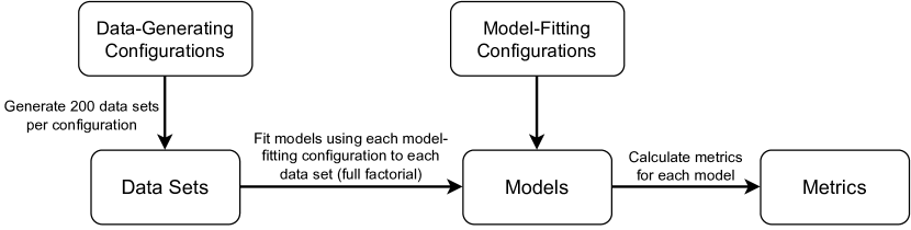
Figure 2: Conceptual simulation architecture. We generated 200 data sets for each entry from a list of data-generating configurations (see Table 1) for a total of $28,800$ datasets. We then fit a model for each entry from a list of model-fitting configurations (see Table 2) to each data set for a total of $1,728,000$ models. Finally, we calculated metrics for all fitted models.

2.1 Causal Foundation

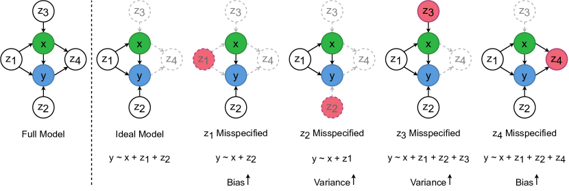
Figure 3: Full data-generating DAG and the resulting models. The ideal model is the subset of the full model that optimally estimates $\beta_{xy}$. Misspecifying with respect to each of the $z_{n}$ variables leads to an additional model, where excluding $z_{1}$ or including $z_{4}$ increases bias, while excluding $z_{2}$ or including $z_{3}$ increases variance of the estimation.

In practice, we usually cannot know if a model actually represents the true DGP, not only in terms of the distributional assumptions of likelihood and link, but also in terms of the structural and causal assumptions of the included (causal) covariates and their (non-)linear combination on the latent space. This uncertainty about covariates and their causal effects is a focus point for the causal literature. As explained in Section 1.1.1, causal consistency is a necessity for good parameter recoverability and thus a fundamental aspect of this study’s methods.

Here, we use a single, prototypical causal directed acyclic graph (DAG; Pearl, 2009a) to guide both data generation and causal model assumptions (see Figure 3). The full DAG displayed on the left-hand side of Figure 3 consists of an outcome $y$, a treatment $x$, and four additional variables $z_{1},z_{2},z_{3},z_{4}$ that correspond to four common, qualitatively different types of controls (Cinelli et al., 2020). With respect to the effect of $x$ on $y$, $z_{1}$ is a fork, $z_{2}$ is an ancestor of $y$, $z_{3}$ is an ancestor of $x$, and $z_{4}$ is a collider. These archetypes represent the majority of controls occurring in reality. The only common control missing from this list is the pipe $(x\rightarrow z\rightarrow y)$, which was not included here due to its similarity with the fork (Cinelli et al., 2020).

The goal of our statistical models will be to estimate the causal effect $\beta_{xy}$ of $x$ on $y$ as accurately as possible. For this purpose, $z_{1}$ constitutes a ’good control’ in the sense that controlling for it decreases bias in the estimation, while $z_{4}$ is a ’bad control’, as controlling for it increases bias. In contrast, $z_{2}$ and $z_{3}$ are ’neutral controls’: controlling for them does not influence bias. However, controlling for $z_{2}$ increases precision (decreases variance) while controlling for $z_{3}$ decreases precision of the estimation of $\beta_{xy}$. As a result, to estimate $\beta_{xy}$, the ideal (causal) model only controls for $z_{1}$ and $z_{2}$ (see the second graph in Figure 3). From there, we can obtain misspecified (causal) models by including or excluding controls. Based on four controls, $2^{4}-1=15$ misspecified models are conceivable, but for simplicity, we focus only on a subset of four of them, each of which deviates from the ideal model in exactly one control (see the third to sixth graph in Figure 3). Two of these misspecified models (i.e., when incorrectly excluding $z_{2}$ or incorrectly including $z_{3}$) still yield (asymptotically) unbiased estimates of $\beta_{xy}$. We will call them and the ideal causal model ’causally unbiased’, while we call (asymptotically) biased models ’causally biased’ (Bürkner et al., 2022a). Using this terminology, we can formulate our primary research questions more precisely as:

1. Within a set of statistical models that all share the same underlying causal model, can prediction be reliably used as a proxy for explanation?

2. Does the answer to (i) depend on whether or not the causal model is biased?

Focusing on these questions implies that we do not aim to compare models with differing linear predictor terms (i.e., causal assumptions as per Figure 3). For one, there already are well known examples of cross-formula comparisons where the alignment of prediction and explanation doesn’t hold (e.g., adding a collider improves prediction but worsens explanation compared to an ideal unbiased model; McElreath, 2020). Still, cross-formula comparison includes a lot of uncharted territory, which we think is worth studying but out of scope of the present paper. Of course, as a result of this choice, we need other aspects to vary among the compared statistical models. In this study, these aspects will be the likelihood and link functions of Bayesian GLMs as detailed next.

2.2 Likelihoods and Link Functions

The range of practically relevant likelihood classes is extensive and encompasses, among others, likelihoods for unbounded, lower-bounded, and double-bounded continuous data, as well as binary, categorical, ordinal, count, and proportional (sum-to-one) data (Johnson et al., 1995, 2005; Stasinopoulos and Rigby, 2007; Yee, 2010; Bürkner, 2021). Studying all of them at once would be too large of a scope for a single paper. Here, we focus our efforts on GLMs with lower-bounded or double-bounded continuous likelihoods. Within these classes, we not only have several qualitatively different (non-nested) likelihood options, but can also study both main classes of non-identity link functions.

Below, we give a short overview of the likelihood and link functions included in the simulations. For consistency, we use mean parameterizations of likelihoods throughout or, if those are unavailable, median parameterizations. A more detailed review of the considered options, our inclusion criteria, and the used parameterizations are available in the supplemental material and online appendix (Scholz and Bürkner, 2022c).

2.2.1 Likelihoods and links for double-bounded responses

Without loss of generality, any double-bounded response can be linearly transformed to the unit interval. Accordingly, it is sufficient to focus on likelihoods for unit interval data. We included the beta (Espinheira et al., 2008), Kumaraswamy (Kumaraswamy, 1980), simplex (Barndorff-Nielsen and Jørgensen, 1991), and transformed-normal (Atchison and Shen, 1980; Kim et al., 2017) likelihoods. The transformed-normal likelihoods arise from applying the link functions to the response variable $y$ (e.g., resulting in the logit-normal likelihood), instead of to the location parameter $\mu$ as would be usual in standard GLMs. All of these likelihoods have two distributional parameters, one location (mean or median) and one scale/shape parameter, only the former being predicted as per the causal graph structures. Figure 4 shows some example densities for each likelihood, illustrating qualitatively different shapes they can accommodate. The three distinct shapes are unimodal symmetric and asymmetric shapes as well as a bimodal bathtub shape. For the remainder of the paper, we will refer to these shapes as symmetric, asymmetric, and bathtub, respectively. As link functions, we included the logit, cloglog, and cauchit links, each of them having qualitatively different properties (Yin et al., 2020; Jiang et al., 2013; Lemonte and Bazán, 2018; Damisa et al., 2017; Fahrmeir et al., 1994; Gill et al., 2001; Powers and Xie, 2008; Morgan and Smith, 1992; Koenker and Yoon, 2009; Lemonte and Bazán, 2018). The logit link is based on the symmetric, light-tailed logistic distribution, the cloglog link is based on the asymmetric Gumbel distribution, while the cauchit link is based on the symmetric, heavy tailed Cauchy distribution. Since logit and probit yield almost indistinguishable results due to the similar shapes of the logistic and normal distributions (Fahrmeir et al., 1994; Gill et al., 2001; Powers and Xie, 2008), we decided against including the probit link despite its prominence.

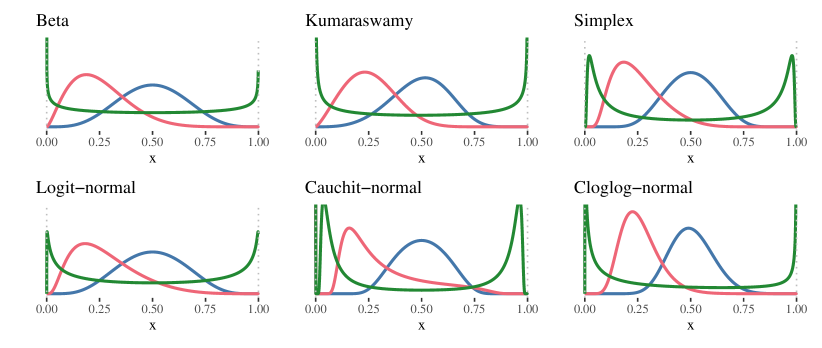
Figure 4: Example illustrations of all included double-bounded densities each with three different shapes. The y-axis is truncated at 5 from above for better visibility of the different shapes.

2.2.2 Likelihoods and links for lower-bounded responses.

Without loss of generality, any continuous lower-bounded response can be linearly transformed to have a lower bound of zero. Accordingly, it is sufficient to focus on likelihoods for strictly positive data. We included the gamma, Weibull, Fréchet, inverse Gaussian, beta prime, Gompertz, and transformed-normal likelihoods all of whom have two distributional parameters, namely location (mean or median) and scale or shape). Figure 5 shows example densities for each likelihood, illustrating qualitatively different kinds of shapes they can accommodate. The three distinct shapes are unimodal thin tail and heavy tail shapes as well as a ramp shape. For the remainder of the paper we will refer to these shapes as thin tail, heavy tail, and ramp, respectively. As link functions, we included the log and the softplus link. In contrast to the multiplicative log link, softplus approaches the identity for larger values, thus approximating additive behavior of regression terms while enforcing positive predictions at the same time (Zheng et al., 2015; Dugas et al., 2000).

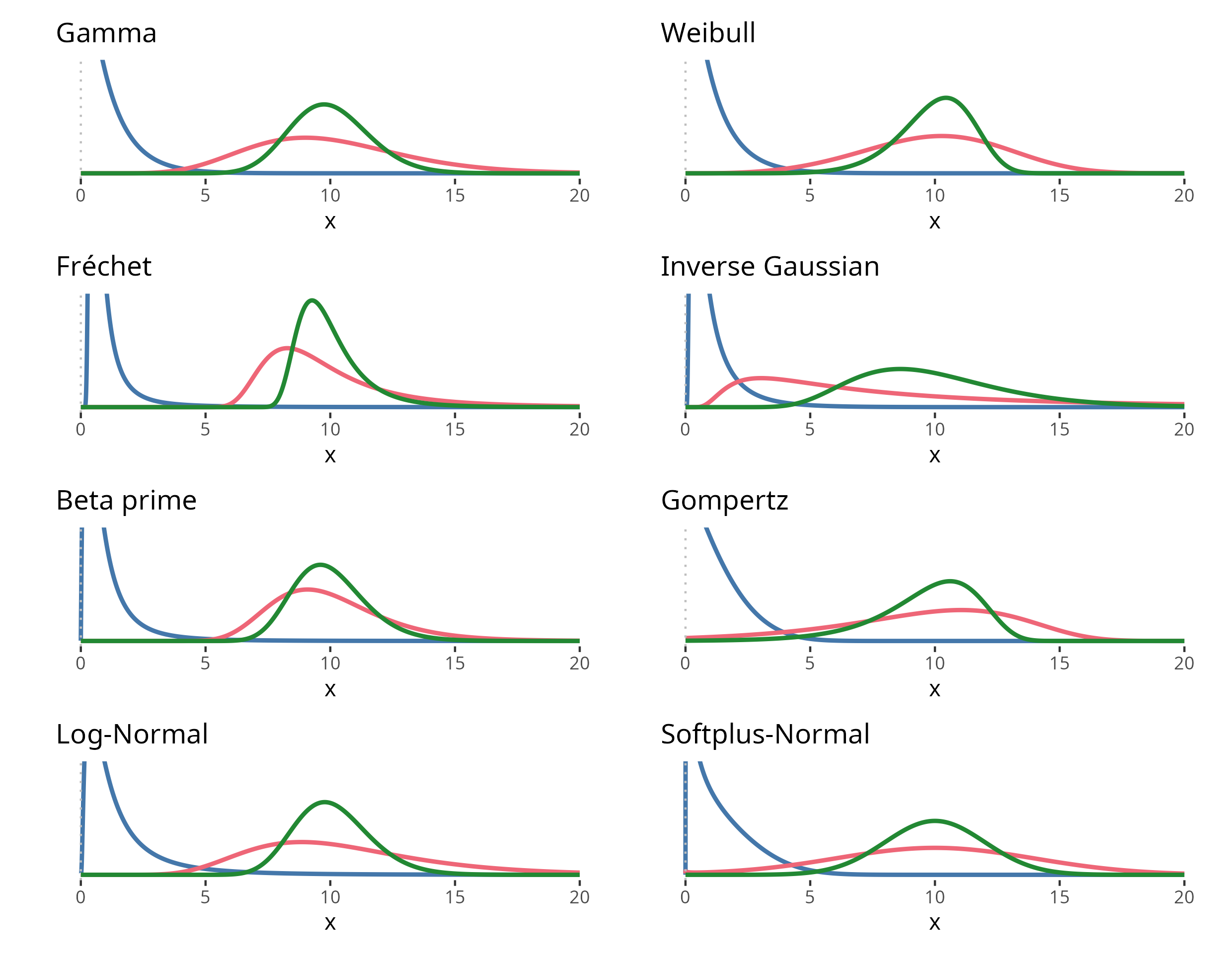
Figure 5: Example illustrations of all included lower-bounded densities, each with three different shapes. The y-axis is truncated at 0.4 from above for better visibility of the different shapes.

2.3 Data Generation

For each of the combinations of likelihood family, likelihood shape, and link presented in Section 2.2, we simulated data sets based on the full DAG (Figure 3 left-hand side) as follows:

$$z_{1} \sim\mathrm{normal}(0,\sigma_{z_{1}}),\quad z_{2}\sim\mathrm{normal}(0,\sigma_{z_{2}}),\quad z_{3}\sim\mathrm{normal}(0,\sigma_{z_{3}})$$

$$x \sim\mathrm{normal}(\beta_{z_{1}x}z_{1}+\beta_{z_{3}x}z_{3},\sigma_{x})$$

$$y \sim\textrm{likelihood}(\textrm{link}^{-1}(\alpha_{y}+\beta_{xy}x+\beta_{z_{1}y}z_{1}+\beta_{z_{2}y}z_{2}),\phi)$$

$$z_{4} \sim\mathrm{normal}(\beta_{xz_{4}}x+\beta_{yz_{4}}y,\sigma_{z_{4}}).$$

Here, $\phi$ denotes the second distributional (scale or shape) parameter of the specified likelihood family and $\textrm{link}^{-1}$ denotes the inverse link (or response-) function. We chose normal distributions to generate all data variables besides $y$ to limit the scope of our simulations. Each simulated data set contained $100$ observations. Since the fitted models only have between 4 and 6 parameters, they are simple enough to be well identified on the basis of $100$ observations alone. The parameters of the true DGP were set to fixed values, rather than being drawn from a prior distribution (Talts et al., 2018), to avoid blurring the effect of the induced causal misspecifications and different likelihood shapes. This decision was made due to the extreme data sets that prior distributions over parameters could create, which is a general challenge for Bayesian simulations (Gabry et al., 2019; Mikkola et al., 2021).

Each likelihood’s second distributional parameter $\phi$ as well as the intercept $\alpha_{y}$ were chosen to produce the shapes presented in Section 2.2. The individual coefficients for $x$ and the $z_{i}$ were calibrated so that the parameter recovery was imperfect for the ideal model while also preventing the causally misspecified models from consistently failing (see also Section 2.4). The true causal effect $\beta_{xy}$ of $x$ on $y$ was either fixed to zero or set to a non-zero value that was calibrated together with all other coefficients. To prevent response values from under- or overflowing to the lower- or upper boundaries numerically, we truncated them near the boundaries around the 6${}^{\text{th}}$ digit.

For each data generation configuration implied by fully crossing the design factors (see Table 1), we generated $200$ data sets, which resulted in $14,400$ data sets each for the double- and single-bounded scenarios.

Table 1: Overview of data generation configurations.

Factor	Levels
Double-bounded likelihoods	beta, Kumaraswamy, simplex, transformed-normal
Double-bounded links	logit, cauchit, cloglog
Double-bounded shapes	symmetric, asymmetric, bathtub
Lower-bounded likelihoods	gamma, Weibull, transformed-normal, Fréchet, beta-prime, Gompertz
Lower-bounded links	log, softplus
Lower-bounded shapes	ramp, heavy tail, thin tail
True $\beta_{xy}$	zero, positive

2.4 Model Fitting

On each generated data set, we fitted all models resulting from the fully crossed combination of likelihoods and links (see Section 2.2) as well as the five different linear predictor terms implied by the ideal and misspecified causal models (see Section 2.1). In reference to R formula syntax, we will also refer to the different linear predictor terms as formulas in the following. Accordingly, given a data set generated from a double-bounded likelihood, we fitted models on that data set using all combinations of double-bounded likelihoods, links, and DAG-based formulas (see Figure 3). The same approach was followed for the lower-bounded data. An overview of the model fit configurations is given in Table 2.

The fully-crossed design results in $60$ fit configurations for the double-bounded and lower-bounded models. Multiplied with $14,400$ data sets each, this leads to a total of $864,000$ double-bounded and single-bounded models each fitted in our simulations.

Table 2: Overview of model fit configurations.

Factor	Levels
Double-bounded Likelihoods	beta, Kumaraswamy, simplex, transformed-normal
Double-bounded Links	logit, cauchit, cloglog
Single-bounded Likelihoods	gamma, Weibull, transformed-normal, Fréchet, beta-prime, Gompertz
Single-bounded Links	log, softplus
Formulas (right-hand side)	$x+z_{1}+z_{2}$, $\;x+z_{2}$, $\;x+z_{1}$, $\;x+z_{1}+z_{2}+z_{3}$, $\;x+z_{1}+z_{2}+z_{4}$

Contrary to what we would recommend in practical applications of Bayesian models, we used flat priors for all model parameters, as it is not clear to us how one would specify equivalent priors for the different auxiliary parameters $\phi$ across all likelihood. What is more, different links imply different latent scales, which render the regression coefficients’ scales incomparable across (assumed) links and thus further complicates equivalent prior specification. In a real-world analysis, we would prefer to use at least weakly-informative priors (Stan Development Team, 2022; Gelman et al., 2013; McElreath, 2020). Accordingly, the current choice is to be understood only in the context of the present simulation study aiming to ensure comparability across likelihoods and links. In pilot experiments (not shown here), we have confirmed that the differences in posteriors as well as the implied prediction metrics between models with flat vs. weakly informative priors are minimal for the models under investigation. We argue that such minimal differences do not justify extensive evaluation of different prior choices, since this is not the focus of the present paper. Additionally, the use of flat priors results in model estimations very similar to maximum likelihood estimation, which is another reason why we expect the results of this study to generalize to frequentist models as well.

All models were fitted using Stan (Carpenter et al., 2017; Stan Development Team, 2022) via brms (Bürkner, 2017) with two chains, 500 warmup- and 2000 post-warmup samples, which resulted in $4000$ total post-warmup posterior samples per model. We used an initialization range of $0.1$ around the origin on the unconstrained parameter space to avoid occasional initialization failures. For all other MCMC hyperparameters, we applied the brms defaults (Bürkner, 2017).

2.5 Model-Based Metrics

To measure parameter recovery and predictive performance of each fitted model, we used multiple metrics as detailed below. Implementations of these metrics are provided in the R packages loo (Vehtari et al., 2022), posterior (Bürkner et al., 2022b), bayesim (Scholz and Bürkner, 2022a), and bayeshear (Scholz and Bürkner, 2022b).

2.5.1 Parameter recoverability

To date, the primary metric for causal parameter recoverability (operationalizing explanation) remains the estimation bias. However, as argued in Section 1.1, it may not be the only sensible metric. Instead, in order to allow for a bias-variance trade-off in the causal estimate’s evaluation, the RMSE may be a worthy alternative metric in non-asymptotic regimes.

More precisely, given a true parameter value $\theta$ and a set of corresponding posterior samples $\{\theta^{(s)}\}$, we compute the sampling-based posterior bias and $\mathrm{RMSE}$ as

$$\mathrm{bias}(\theta^{(s)}):=\frac{1}{S}\sum^{S}_{s=1}\left(\theta^{(s)}\right)-\theta,$$ (1)

$$\mathrm{RMSE}(\theta^{(s)}):=\sqrt{\frac{1}{S}\sum^{S}_{s=1}\left((\theta^{(s)}-\theta)^{2}\right)}=\sqrt{\mathrm{bias}(\theta^{(s)})^{2}+\mathrm{Var}\left(\theta^{(s)}\right)},$$ (2)

where $\mathrm{Var}(\theta^{(s)})$ denotes the variance over the posterior samples. Our analysis focuses on the true causal effect $\beta_{xy}$ and hence all metrics were computed for $\theta=\beta_{xy}$. Furthermore, as we are interested in the size of the bias but not in its direction, we will present the absolute bias in our results.

The above are reasonable measures for comparing models only if the assumed link coincides with the true link of the DGP. This is because the link determines the scale of the linear predictor and thus the comparability of the posterior samples $\{\beta_{xy}^{(s)}\}$ with the true parameter value $\beta_{xy}$. To enable a comparison of models using different links, we also calculated the false positive rate (FPR; i.e., Type I-error rate) and the true positive rate (TPR; i.e., statistical power; inverse of the Type II-error rate) implied by the central 95% credible interval of $\{\beta_{xy}^{(s)}\}$. These metrics can be inferred from our simulations, because the true causal effect $\beta_{xy}$ was set to zero in some conditions (to study FPR) and to non-zero values in others (to study TPR).

2.5.2 Predictive performance

In the absence of any case-specific arguments for a particular predictive metric, log-probability scores are recommended as a general-purpose choice (Vehtari et al., 2017). For this reason, we computed the expected log pointwise predictive density ($\mathrm{ELPD}$; Vehtari and Ojanen, 2012; Vehtari et al., 2017) as our main metric for predictive performance (operationalizing prediction), which is defined as

$$\text{ELPD}(y^{*}):=\sum_{i=1}^{N^{*}}\log p(y^{*}_{i}\mid\tilde{y})=\sum_{i=1}^{N^{*}}\log\left(\frac{1}{S}\sum^{S}_{s=1}p(y^{*}_{i}\,|\,\theta^{(s)})\right),$$ (3)

where $\tilde{y}$ denotes the training data and $y^{*}$ denotes $N^{*}=100$ independent test data points (previously unseen by the model) simulated from the same DGP configuration as the training data. We refer to the above metric as $\mathrm{ELPD}_{\rm test}$. In addition, we also calculated $\mathrm{ELPD}$ via leave-one-out cross-validation (LOO-CV) as approximated via Pareto-smoothed importance sampling (PSIS; Vehtari et al., 2017, 2022). We refer to this metric as $\mathrm{ELPD}_{\rm loo}$. Approximate LOO-CV metrics have the advantage that they are readily and efficiently available also when analysing real data, at the expense of being only an approximation that might fail to estimate out-of-sample predictive performance accurately if there are influential observations (Vehtari et al., 2017). The $\mathrm{ELPD}_{\rm test}$ metric is usually not available during real-world inference due to the absence of independent test data, so we mainly used it to validate the approximate $\mathrm{ELPD}_{\rm loo}$ results.

In order to compare multiple models with respect to their ELPD performance, we calculated the $\mathrm{ELPD}$ difference to the best performing model from a set $M:=\{m_{1},...,m_{K}\}$ of $K$ models all fit to the same training data:

$$\Delta\mathrm{ELPD}(y^{*}\mid m_{i}):=\mathrm{ELPD}(y^{*}\mid m_{i})-\text{max}(\mathrm{ELPD}(y^{*}\mid M)).$$ (4)

As explained in Section 2.1, we always restricted comparisons (i.e., $M$) to models that used the same linear predictor. Additionally, for investigating posterior bias and RMSE performance, only models assuming the correct link function were compared.

2.6 Statistical Analysis

To analyse the relationship between predictive performance, as measured by $\Delta\mathrm{ELPD}_{\rm loo}$ and $\Delta\mathrm{ELPD}_{\rm test}$, and parameter recoverability, as measured by absolute bias, RMSE, FPR, and TPR, we modeled the simulation results via Bayesian multilevel-models (BMMs).

Simulation results of models that did not converge were excluded from the analysis. Specifically, we treated models as converged if the posterior samples $\{\beta_{xy}^{(s)}\}$ yielded $\widehat{R}<1.01$ and $\mathrm{ESS}>400$ (for details on these thresholds, see Vehtari et al., 2021). What is more, we required models to have less than $10$ divergent transitions out of a total of 4000 post-warmup iterations. Ideally, we would like all models to converge with no divergent transitions, but this would have required extensive manual intervention to resolve all individual sampling problems, which is practically infeasible in our large simulation setup. Within the set of convergent models, PSIS diagnostics indicated good $\mathrm{ELPD}_{\rm loo}$ approximations such that the latter can be treated as a trustworthy estimate of out-of-sample predictive performance (Vehtari et al., 2017). Finally, we set a lower threshold $\Delta\mathrm{ELPD}_{\rm loo}>-N\,(\,=-100)$ to exclude models that made exceptionally bad predictions compared to the best performing model on a given data set. This resulted in apprimately 7% of models being filtered from the results. Most of the filtered models (i.e., of the the approximately 7%) from the double-bounded results were fit on data generated from a bathtub link (73%) and filtered due to missing the $\Delta\mathrm{ELPD}_{\rm loo}$ threshold (94%). For the lower-bounded models, most filtered models failed to meet our convergence criteria (74%) and were fit using a softplus link (73%) and Fréchet likelihood.

In the linear predictor term of the BMMs, we included overall (’fixed’) effects of $\Delta\mathrm{ELPD}$ in interaction with formula (i.e., the linear predictor term), (true) data generating link, and data generating shape, which we refer to as the global slopes in the results in Section 3. Additionally, to account for the dependency of results obtained from the same simulated data set, we included varying (’random’) effects across data sets of $\Delta\mathrm{ELPD}$ in interaction with formula which we refer to as the varying slopes in the results in Section 3. For the continuous positive metrics of parameter recovery, that is, absolute bias and RMSE, we assumed a log-normal likelihood, which enabled the use of highly optimized (log-)linear regression functions in Stan (Stan Development Team, 2022). For the binary metrics, that is, FPR and TPR, we assumed a canonical Bernoulli likelihood with logit link. The BMMs were estimated using a single MCMC chain with $500$ warmup and $1000$ post-warmup samples to keep the estimation time manageable (between one and three days wall-clock time per BMM). All convergence metrics indicated sufficient convergence. As we were mainly interested in the qualitative patterns, rather than high resolution numerical results, we considered $1000$ post-warmup samples as sufficient, leading to effective sample sizes of a few hundred.

3 Results

Recall, that this paper consists of two levels of Bayesian models. The first level are the models from the simulation study, that were fittet on simulated data as described in Section 2.4. The second level are meta-models that we fit on the metrics we extracted from the first level as described in Section 2.6. All results presented in this section are based on the meta-models to learn about trends across the entire simulation study. Due to the vast number of simulation conditions, the main text illustrates selected results which are representative of the key patterns in the full simulation. The full results are available in the supplementary material and in the online appendix (Scholz and Bürkner, 2022c). In preliminary comparisons of $\mathrm{ELPD}_{\rm loo}$ and $\mathrm{ELPD}_{\rm test}$ results, we found both to be highly similar. What is more, Pareto-$\hat{k}$ values of the $\mathrm{ELPD}_{\rm loo}$ approximation were generally low indicating good approximation accuracy (Vehtari et al., 2017). For these reasons, we only present results of $\mathrm{ELPD}_{\rm loo}$ below due to its availability during real-world inference. Further, we do not present results for $|\mathrm{bias}(\beta_{xy}^{(s)})|$ here, as they show the same qualitative trends as $\mathrm{RMSE}(\beta_{xy}^{(s)})$. Similarly, we will generally only show examples for either the double- or the lower-bounded data when the conclusions drawn from them match. Some of the presented results show floor or ceiling effects, which point to a suboptimal hyperparameter calibration, discussed in more detail in Section 4.

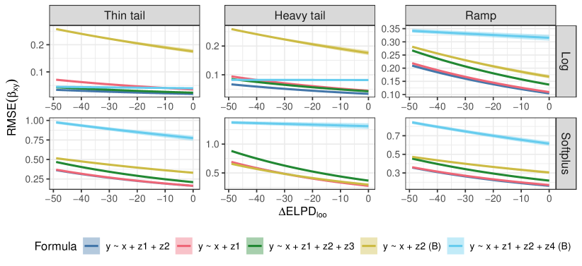
Figure 6: Global slopes of $\Delta\mathrm{ELPD}_{\rm loo}$ on $\mathrm{RMSE}(\beta_{xy}^{(s)})$ for lower-bounded data and models. The shaded area represents the 95% credible intervals of the posterior. The results are split by data generating link and shape as well as colored by formula, where (B) indicates the causally biased formulas. The x-axis is truncated at $-50$ to prevent unreasonable extrapolation to sparse data spaces. The negative slopes for causally unbiased formulas indicate improved RMSE for better predicting models.

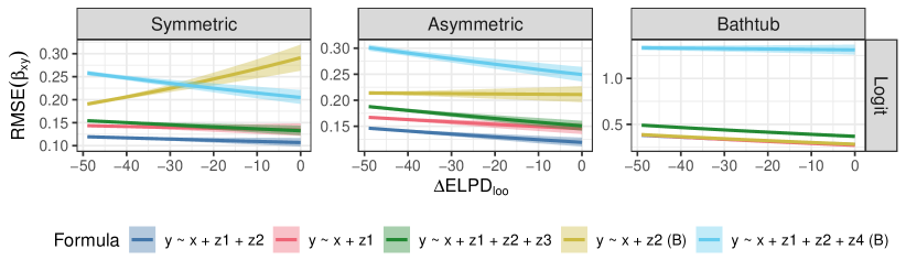
Figure 7: Global slopes of of $\Delta\mathrm{ELPD}_{\rm loo}$ on $\mathrm{RMSE}(\beta_{xy}^{(s)})$ for double-bounded models and data generated with a logit link. The shaded area represents the 95% credible intervals of the posterior. The results are split by data generating shape and colored by formula, where (B) indicates the causally biased formulas. The x-axis is truncated at $-50$ to prevent unreasonable extrapolation to sparse data spaces. The negative slopes for causally unbiased formulas indicate improved RMSE for better predicting models.

3.1 RMSE

Figure 6 displays the global slopes of $\Delta\mathrm{ELPD}_{\rm loo}$ on $\mathrm{RMSE}(\beta_{xy}^{(s)})$ for the lower-bounded data, grouped by formula (i.e., linear predictor), data generating link, and shape as explained in Section 2.6. The most important observation is that all slopes of unbiased formulas were negative, often very strongly so. This means that, within a set of models fitted to the same data set and assuming the same causally unbiased formula, models that have higher (better) $\Delta\mathrm{ELPD}_{\rm loo}$ can be expected to have substantially lower (better) $\mathrm{RMSE}(\beta_{xy}^{(s)})$. While the exact size of the improvement is dependent on the simulation’s hyperparameters, $\mathrm{RMSE}(\beta_{xy}^{(s)})$ reduces by around 50% over the displayed span of $\Delta\mathrm{ELPD}_{\rm loo}$, an improvement of the same order of magnitude as the true effect $\beta_{xy}$. Results of the double-bounded models showed the same behaviour. For both data types, some of the unbiased formulas have rather flat slopes. This results from a floor effect in the $\mathrm{RMSE}$, as slopes for formulas that generally have a small error have little room to decrease further. The causally biased formulas are less consistent, with some scenarios even showing positive slopes as exemplarily shown in Figure 7 for double-bounded models fit on logit data. Additionally, even though the generally higher $\mathrm{RMSE}(\beta_{xy}^{(s)})$ of biased formulas would allow for steeper negative slopes, the biased slopes are often similar or even less negative than the unbiased ones.

In Table 3.1, we show the proportion of negative varying slopes across individual data. Similarly to the global slopes, the varying slopes of the unbiased formulas were largely negative (between 95% and 99% of the varying slopes were negative for the lower-bounded data and between 63% and 94% were negative for the double-bounded data). The exact proportion of negative slopes differed somewhat between ground-truth scenarios, as a result of specific hyperparameters choices in the calibration as well as random noise induced by the simulations. However, the generally high proportions of negative varying slopes for the unbiased formulas indicates that the trend of lower (better) $\mathrm{RMSE}(\beta_{xy}^{(s)})$ for higher (better) $\Delta\mathrm{ELPD}_{\rm loo}$ is consistent across data sets. For the causally biased formulas, the proportion of negative varying slopes were generally lower than for the unbiased formulas for each ground truth. In addition to those general trends, the proportion of negative slopes for the double-bounded models showed more variability between ground truths than the lower-bounded data. Especially the logit link had a lower proportion than the other scenarios as a result of floor effects.

Proportion of negative varying slopes of $\Delta\mathrm{ELPD}_{\rm loo}$ on $\mathrm{RMSE}(\beta_{xy}^{(s)})$ for individual data sets (higher is better). Log Softplus Thin Tail Heavy Tail Ramp Thin Tail Heavy Tail Ramp Unbiased 0.95 0.96 0.96 0.97 0.99 0.96 Biased 0.69 0.59 0.67 0.76 0.71 0.79

	Logit				Cauchit				Cloglog
	Sym	Asym	BT		Sym	Asym	BT		Sym	Asym	BT
Unbiased	$0.63^{*}$	0.69	0.76		0.9	0.88	0.91		0.83	0.78	0.94
Biased	0.51	0.66	0.64		0.9	0.89	0.92		0.73	0.73	0.93

• ^∗ Floor effects in the global slopes were present for at least one of the respective formulas.

3.2 FPR and TPR

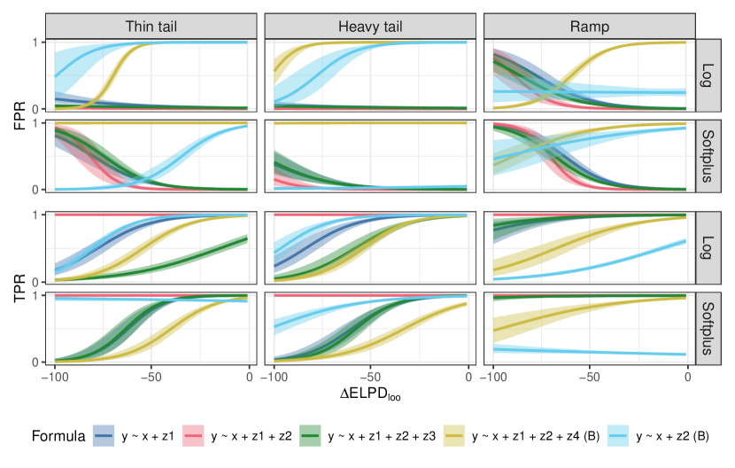
Figure 8: Global slopes of $\Delta\mathrm{ELPD}_{\rm loo}$ on the false positive and true positive rates (FPR and TPR) for lower-bounded data. The shaded area represents the 95% credible intervals of the posterior. The results are split by data generating link and shape as well as colored by formula, where (B) indicates the causally biased formulas. The low FPR and positive TPR slopes of the unbiased formulas indicate better Calibration for better predicting models.

Figure 8 shows the global slopes of $\Delta\mathrm{ELPD}_{\rm loo}$ on FPR and TPR for the lower-bounded data grouped by formula, data generating link, and shape as explained in Section 2.6. Starting with the FPR slopes, there is a clear distinction between the biased and unbiased formulas. Where the unbiased formulas have negative slopes or even stay constant near $0.05$ (nominal Type-I error rate), the biased formulas have positive slopes or stay constant near 1 (i.e., $100$% Type-I error rate) in all cases. The results for the double-bounded scenarios show the same pattern. Acceptable FPR (i.e., values close to or less than the desired Type-I error rate) is a requirement for using TPR as a measure of parameter recovery, because it is trivial to achieve high TPR if FPR is allowed to be high at the same time. Accordingly, while the low FPR for the unbiased formulas implies the usefulness of TPR in these cases, the high FPR for the biased formulas makes their TPR results much less meaningful.

In the TPR results, we found a clear pattern of positive global slopes for the unbiased formulas whenever there are no ceiling effects (i.e., TPR = 1 regardless of $\Delta\mathrm{ELPD}_{\rm loo}$). This indicates, that within models fitted to the same data set and using the same causally unbiased formula, models with higher (better) $\Delta\mathrm{ELPD}_{\rm loo}$ can be expected to have substantially higher (better) TPR. The biased formulas again are less consistent in their slopes with cases of negative global slopes or shallower slopes even for generally low TPR, such that ceiling effects are not an issue. Results of the double-bounded models showed the same behaviour with some additional cases of floor effects.

In Table 8, we show the proportion of positive varying slopes across individual data sets for the TPR. For the causally unbiased formulas, the majority of the varying slopes are strongly positive, such that within a set of models fitted to the same data set and assuming the same causally unbiased formula, models that ranked higher in $\Delta\mathrm{ELPD}_{\rm loo}$ can be expected to have a higher TPR. This effect is rather consistent with positive proportions between $86\%$ and $95\%$ for different ground truths, besides the ramp and bathtub shape. The lower proportion of positive slopes for the ramp and bathtub shapes coincide with the floor and ceiling effects visible in Figure 8.

The biased formulas showed less consistency of the varying slope signs in the lower-bounded scenarios and similar consistency in the double-bounded scenarios.

Proportion of positive varying slopes of $\Delta\mathrm{ELPD}_{\rm loo}$ on TPR (higher is better). Log Softplus Thin Tail Heavy Tail Ramp Thin Tail Heavy Tail Ramp Unbiased 0.78 0.86 0.71 0.92 0.87 $0.61^{*}$ Biased $0.7^{*}$ $0.59^{*}$ $0.51^{*}$ $0.54^{*}$ $0.65^{*}$ $0.25^{*}$

	Logit				Cauchit				Cloglog
	Sym	Asym	BT		Sym	Asym	BT		Sym	Asym	BT
Unbiased	0.94	0.93	$0.24^{*}$		0.95	0.93	$0.78^{*}$		$0.86^{*}$	0.94	$0.74^{*}$
Biased	$0.94^{*}$	$0.94^{*}$	0.81		$0.96^{*}$	$0.88^{*}$	$0.87^{*}$		$0.48^{*}$	$0.93^{*}$	0.55

• ^∗ Floor or ceiling effects in the global slopes were present for at least one of the respective formulas.

4 Discussion

In this paper, we studied the use of prediction as a proxy for explanation under several causal and statistical misspecification mechanisms in Bayesian GLMs. We split our research question into two parts:

1. Within a set of statistical models that all share the same underlying causal model, can prediction be reliably used as a proxy for explanation?

2. Does the answer to (i) depend on whether or not the causal model is biased?

Within our results, we observed one consistent trend over almost all investigated scenarios: When comparing statistical models sharing the same underlying unbiased causal model, all considered measures of explanation (the causal parameter’s absolute bias, RMSE, true positive rate and false positive rate) improved with improving out-of-sample prediction (measured by the expected log predictive density). What is more, in almost all scenarios, the trends were also highly consistent across individual data sets, which indicates that the proxy can be reliably applied in practice, where inference usually concerns a single data set only. In the few causally unbiased cases without a clear trend, the relationship was effectively zero due to floor and ceiling effects (further discussed below). While better predicting models did not necessarily provide better explanation in those cases, prediction was (on average across datasets) not worsening explanation either. For statistical models sharing the same underlying biased causal model, the trends where inconsistent with examples for both improving and degrading explanation with improving prediction. We conclude that, given a set of GLMs that all share the same unbiased causal model, prediction can be safely used as a proxy for explanation.

Our findings also offer empirical support for the more conceptual arguments of Yarkoni and Westfall (2017) and Breiman (2001) that called for more attention to better predicting models, even if explanation is the main goal. In that way, causality seems to be the missing link that connects the statistical relationship of explanation and prediction.

As is typical of simulation studies, their generalizability beyond the studied scenarios should be treated with caution. While an analytic investigation supplementing the simulations would have been desirable, the lack of available closed-form posteriors outside of a few conjugate cases prevented such an investigation (as does the iterative nature of maximum likelihood in the models’ frequentist counterparts). We understand this paper as a promising starting point for further work on the relationship between explanation and prediction under different causal and statistical assumptions. Below, we offer our perspective on subsequent research questions.

As discussed in Section 1.2, we limited the scope of this paper to models with simple linear predictor terms. We would expect to observe the same general trends for more complicated additive predictor terms where individual components may be non-linear, as the DAG-based misspecifications are agnostic to the details of the statistical model structure (Pearl, 2009b). However, investigating the implications of (mis-)specifying individual terms of the linear predictor (e.g., modeling an effect as linear while it is truly non-linear in some way) might be interesting. This would more strongly play into the question of overfitting in sparse scenarios with (relatively) small data yet complicated non-linear relationships to be approximated. Similar questions would arise when adding multilevel structure especially in sparse data scenarios where the (true) relevance of multilevel terms need to be balanced against their weak identification implied by the given data (Gelman and Hill, 2006; Bürkner et al., 2022a).

With regard to causal assumptions, we chose our data-generating processes (DGPs) and the four misspecified linear predictors in an attempt to span the most important and common classes of controls (Cinelli et al., 2020). Still, there remain many other possible DGPs and misspecifications, for example, unobserved variables or variables with measurement error (Kuroki and Pearl, 2014; Tchetgen et al., 2020). An extension of this work to different kinds of DGPs and misspecifications would ultimately add to the generalizability of results. That said, we currently do not see how an unbiased causal model would have to look like in order to render the relationship of prediction and explanation negative (i.e., better predicition implying worse explanation), as long as all compared models all shared the same unbiased causal model.

In contrast, when comparing models with different underlying causal models, the relationship between prediction and explanation is still not fully understood. Even though it is known, for example, that including colliders improves prediction but worsens explanation (McElreath, 2020), the situation for a set of different but all unbiased causal models has not yet been systematically explored to our knowledge. That is, when all compared statistical models have underlying unbiased causal models, it is unclear if improved prediction implies improved explanation if the causal models are allowed to vary across the statistical models. We believe that this research direction would be one of the most important extensions of the present work.

In addition to the influence of the true and assumed causal models, we observed a noticeable effect of the true likelihood shapes assumed in our simulations. The mechanisms by which different shapes imply different downstream results, including the extend of the relationship between prediction and explanation, remain somewhat unclear to us. While the investigation of additional DGPs would generally offer potential for improving the generalizability of our findings, an extension of this work that would especially focus on different data-generating shapes and their properties more systematically could improve said understanding. This directly ties into the problem of choosing reasonable ground-truth model parameters for the simulations. Fully Bayesian simulations tend to struggle when drawing parameters from prior distributions as this can easily lead to extreme and unrealistic data sets (Gabry et al., 2019; Mikkola et al., 2021). Our solution of carefully crafting scenarios that would represent specific, distinct, but still realistic, ground truths comes with the challenge of choosing an overwhelming amount of parameters. This did not fully succeed in all cases, as shown by the floor and ceiling effects that were present in a few scenarios, specifically for the true and false positive rates where causal relationships were sometimes too easy or too hard to detect. While results influenced by those effects still support our overall conclusions, they reduce what we can learn from the affected scenarios.

Finally, in this study, we followed a Bayesian perspective on model building, despite using flat priors. The latter choice was primarily made to avoid some models having an ’unfair’ advantage due to incidentally more suitable prior choices (see Section 2.4). As a side effect of this choice, we think that our main results are likely to hold as well in case of frequentist (maximum likelihood) estimation of all models, and corresponding model-based metrics. We see it as unlikely that our conclusions would have changed in the light of applying (weakly-)informative priors (Stan Development Team, 2022; McElreath, 2020; Gelman et al., 2013). However, there may be one subtle place where priors (or regularization more generally) may influence the relationship between prediction and explanation: Cross-validation measures of out-of-sample prediction produce correlated folds due to overlap in training data and have an intricate relationship with different true quantities they can be seen to approximate (Bates et al., 2021). These properties can be altered via regularization, especially in sparse regimes where the number of model parameters is high relative to the number of observations in the data (Bates et al., 2021). As such, the relationship between prediction and explanation may also vary in such scenarios, which would be interesting to study in the future.

Funding

This work was partially funded by the Deutsche Forschungsgemeinschaft (DFG, German Research Foundation) under Germany’s Excellence Strategy – EXC-2075 - 390740016 (the Stuttgart Cluster of Excellence SimTech).

This work was performed on the computational resource bwUniCluster funded by the Ministry of Science, Research and the Arts Baden-Württemberg and the Universities of the State of Baden-Württemberg, Germany, within the framework program bwHPC.

The authors gratefully acknowledge the support and funding.

Data availability

The data that support the findings of this study are openly available in OSF at http://doi.org/10.17605/OSF.IO/XGKZV.

References

- Gelman et al. [2013] Andrew Gelman, John B. Carlin, Hal S. Stern, David B. Dunson, Aki Vehtari, and Donald B. Rubin. Bayesian Data Analysis. Chapman and Hall/CRC, New York, 3 edition, July 2013. ISBN 978-0-429-11307-9. doi:10.1201/b16018.
- McElreath [2020] Richard McElreath. Statistical Rethinking: A Bayesian Course with Examples in R and Stan. Chapman and Hall/CRC, New York, 2 edition, March 2020. ISBN 978-0-429-02960-8. doi:10.1201/9780429029608.
- Gelman et al. [2020a] Andrew Gelman, Aki Vehtari, Daniel Simpson, Charles C. Margossian, Bob Carpenter, Yuling Yao, Lauren Kennedy, Jonah Gabry, Paul-Christian Bürkner, and Martin Modrák. Bayesian Workflow. arXiv:2011.01808 [stat], November 2020a. arXiv: 2011.01808.
- Scholz and Bürkner [2022a] Maximilian Scholz and Paul-Christian Bürkner. Bayesim: Framework for bayesian simulation studies, 2022a. URL https://github.com/sims1253/bayesim. R package version 0.29.5.9000.
- Scholz et al. [2022] Maximilian Scholz, Yannick Dzubba, and Paul-Christian Bürkner. bayesfam: Custom families for brms, 2022. URL https://github.com/sims1253/bayesfam. R package version 0.2.4.
- Scholz and Bürkner [2022b] Maximilian Scholz and Paul-Christian Bürkner. bayeshear: Toolbox of bayesian model metrics, 2022b. URL https://github.com/sims1253/bayeshear. R package version 0.2.0.9000.
- Douglas [2009] Heather E Douglas. Reintroducing prediction to explanation. Philosophy of Science, 76(4):444–463, 2009.
- Bürkner et al. [2022a] Paul-Christian Bürkner, Maximilian Scholz, and Stefan T. Radev. What makes a good bayesian model? towards a unified model taxonomy. arXiv preprint, 2022a.
- Hastie et al. [2009] Trevor Hastie, Robert Tibshirani, Jerome H Friedman, and Jerome H Friedman. The elements of statistical learning: data mining, inference, and prediction, volume 2. Springer, 2009.
- Gabaix and Laibson [2008] Xavier Gabaix and David Laibson. The seven properties of good models. The foundations of positive and normative economics: A handbook, pages 292–319, 2008.
- Vehtari and Ojanen [2012] Aki Vehtari and Janne Ojanen. A survey of Bayesian predictive methods for model assessment, selection and comparison. Statistics Surveys, 6(none):142–228, January 2012. ISSN 1935-7516. doi:10.1214/12-SS102.
- Vehtari et al. [2017] Aki Vehtari, Andrew Gelman, and Jonah Gabry. Practical bayesian model evaluation using leave-one-out cross-validation and waic. Statistics and computing, 27(5):1413–1432, 2017.
- Pearl [2009a] Judea Pearl. Causality. Cambridge University Press, 2009a.
- Pearl [2012] Judea Pearl. The do-calculus revisited. arXiv preprint arXiv:1210.4852, 2012.
- Rubin [1974] Donald B Rubin. Estimating causal effects of treatments in randomized and nonrandomized studies. Journal of Educational Psychology, 66(5):688, 1974.
- Rubin [1978] Donald B Rubin. Bayesian inference for causal effects: The role of randomization. The Annals of Statistics, pages 34–58, 1978.
- Shmueli [2010] Galit Shmueli. To Explain or to Predict? Statistical Science, 25(3), August 2010. ISSN 0883-4237. doi:10.1214/10-STS330.
- Henckel et al. [2022] Leonard Henckel, Emilija Perković, and Marloes H Maathuis. Graphical criteria for efficient total effect estimation via adjustment in causal linear models. Journal of the Royal Statistical Society Series B, 84(2):579–599, 2022.
- Rotnitzky and Smucler [2020] Andrea Rotnitzky and Ezequiel Smucler. Efficient adjustment sets for population average causal treatment effect estimation in graphical models. The Journal of Machine Learning Research, 21(1):7642–7727, 2020.
- Cinelli et al. [2020] Carlos Cinelli, Andrew Forney, and Judea Pearl. A Crash Course in Good and Bad Controls. SSRN Electronic Journal, 2020. ISSN 1556-5068. doi:10.2139/ssrn.3689437.
- Ramspek et al. [2021] Chava L Ramspek, Ewout W Steyerberg, Richard D Riley, Frits R Rosendaal, Olaf M Dekkers, Friedo W Dekker, and Merel van Diepen. Prediction or causality? a scoping review of their conflation within current observational research. European journal of epidemiology, 36:889–898, 2021.
- Navarro [2019] Danielle J. Navarro. Between the Devil and the Deep Blue Sea: Tensions Between Scientific Judgement and Statistical Model Selection. Computational Brain & Behavior, 2(1):28–34, March 2019. ISSN 2522-087X. doi:10.1007/s42113-018-0019-z.
- Hernán et al. [2019] Miguel A Hernán, John Hsu, and Brian Healy. A second chance to get causal inference right: a classification of data science tasks. Chance, 32(1):42–49, 2019.
- Yarkoni and Westfall [2017] Tal Yarkoni and Jacob Westfall. Choosing Prediction Over Explanation in Psychology: Lessons From Machine Learning. Perspectives on Psychological Science, 12(6):1100–1122, November 2017. ISSN 1745-6916, 1745-6924. doi:10.1177/1745691617693393.
- Breiman [2001] Leo Breiman. Statistical Modeling: The Two Cultures (with comments and a rejoinder by the author). Statistical Science, 16(3):199–231, August 2001. ISSN 0883-4237, 2168-8745. doi:10.1214/ss/1009213726. Publisher: Institute of Mathematical Statistics.
- Cranmer and Desmarais [2017] Skyler J Cranmer and Bruce A Desmarais. What can we learn from predictive modeling? Political Analysis, 25(2):145–166, 2017.
- Gilpin et al. [2018] Leilani H Gilpin, David Bau, Ben Z Yuan, Ayesha Bajwa, Michael Specter, and Lalana Kagal. Explaining explanations: An overview of interpretability of machine learning. In 2018 IEEE 5th International Conference on data science and advanced analytics (DSAA), pages 80–89. IEEE, 2018.
- Carvalho et al. [2019] Diogo V Carvalho, Eduardo M Pereira, and Jaime S Cardoso. Machine learning interpretability: A survey on methods and metrics. Electronics, 8(8):832, 2019.
- Li et al. [2022] Jia Li, Xiaowei Jia, Haoyu Yang, Vipin Kumar, Michael Steinbach, and Gyorgy Simon. Incorporating causal effects into deep learning predictions on ehr data. arXiv preprint arXiv:2011.05466, 2022.
- Richens et al. [2020] Jonathan G Richens, Ciarán M Lee, and Saurabh Johri. Improving the accuracy of medical diagnosis with causal machine learning. Nature communications, 11(1):3923, 2020.
- Schölkopf [2022] Bernhard Schölkopf. Causality for Machine Learning, page 765–804. Association for Computing Machinery, New York, NY, USA, 1 edition, 2022. ISBN 9781450395861. URL https://doi.org/10.1145/3501714.3501755.
- Raissi et al. [2019] Maziar Raissi, Paris Perdikaris, and George E Karniadakis. Physics-informed neural networks: A deep learning framework for solving forward and inverse problems involving nonlinear partial differential equations. Journal of Computational physics, 378:686–707, 2019.
- Karniadakis et al. [2021] George Em Karniadakis, Ioannis G Kevrekidis, Lu Lu, Paris Perdikaris, Sifan Wang, and Liu Yang. Physics-informed machine learning. Nature Reviews Physics, 3(6):422–440, 2021.
- Arrieta et al. [2020] Alejandro Barredo Arrieta, Natalia Díaz-Rodríguez, Javier Del Ser, Adrien Bennetot, Siham Tabik, Alberto Barbado, Salvador García, Sergio Gil-López, Daniel Molina, Richard Benjamins, et al. Explainable artificial intelligence (xai): Concepts, taxonomies, opportunities and challenges toward responsible ai. Information fusion, 58:82–115, 2020.
- Lundberg and Lee [2017] Scott M Lundberg and Su-In Lee. A unified approach to interpreting model predictions. Advances in neural information processing systems, 30, 2017.
- Ribeiro et al. [2016] Marco Tulio Ribeiro, Sameer Singh, and Carlos Guestrin. "why should I trust you?": Explaining the predictions of any classifier. In Proceedings of the 22nd ACM SIGKDD International Conference on Knowledge Discovery and Data Mining, San Francisco, CA, USA, August 13-17, 2016, pages 1135–1144, 2016.
- Watanabe [2009] Sumio Watanabe. Algebraic geometry and statistical learning theory, volume 25. Cambridge university press, 2009.
- Spiegelhalter et al. [1998] David J Spiegelhalter, Nicola G Best, Bradley P Carlin, and A Van der Linde. Bayesian deviance, the effective number of parameters, and the comparison of arbitrarily complex models. Technical report, Citeseer, 1998.
- Watanabe and Opper [2010] Sumio Watanabe and Manfred Opper. Asymptotic equivalence of Bayes cross validation and widely applicable information criterion in singular learning theory. Journal of machine learning research, 11(12), 2010.
- Betancourt [2020] Michael Betancourt. Towards a principled bayesian workflow, 2020. URL https://betanalpha.github.io/assets/case_studies/principled_bayesian_workflow.html.
- Hagerty and Srinivasan [1991] Michael R Hagerty and V Srinivasan. Comparing the predictive powers of alternative multiple regression models. Psychometrika, 56(1):77–85, 1991.
- Gelman et al. [2020b] Andrew Gelman, Jennifer Hill, and Aki Vehtari. Regression and other stories. Cambridge University Press, 2020b.
- Harrell [2015] Frank E Harrell. Regression modeling strategies: with applications to linear models, logistic and ordinal regression, and survival analysis. Springer, 2015.
- Nelder and Wedderburn [1972] John Ashworth Nelder and Robert WM Wedderburn. Generalized linear models. Journal of the Royal Statistical Society: Series A (General), 135(3):370–384, 1972. Publisher: Wiley Online Library.
- Gill et al. [2001] Jeff Gill, Jefferson M Gill, Michelle Torres, and Silvia Michelle Torres Pacheco. Generalized linear models: a unified approach, volume 134. Sage Publications, 2001.
- Bates et al. [2015] Douglas Bates, Martin Mächler, Ben Bolker, and Steve Walker. Fitting Linear Mixed-Effects Models Using \pkglme4. Journal of Statistical Software, 67(1):1–48, 2015.
- Bürkner [2017] Paul-Christian Bürkner. brms: An r package for bayesian multilevel models using stan. Journal of statistical software, 80:1–28, 2017.
- Gelman et al. [2017] Andrew Gelman, Daniel Simpson, and Michael Betancourt. The prior can often only be understood in the context of the likelihood. Entropy, 19(10):555–567, 2017. Publisher: Multidisciplinary Digital Publishing Institute.
- R Core Team [2018] R Core Team. R: A Language and Environment for Statistical Computing. R Foundation for Statistical Computing, Vienna, Austria, 2018. URL https://www.R-project.org/.
- Stan Development Team [2022] Stan Development Team. Stan modeling language users guide and reference manual, 2.30.0, 2022. URL https://mc-stan.org.
- Carpenter et al. [2017] Bob Carpenter, Andrew Gelman, Matthew D Hoffman, Daniel Lee, Ben Goodrich, Michael Betancourt, Marcus Brubaker, Jiqiang Guo, Peter Li, and Allen Riddell. Stan: A probabilistic programming language. Journal of statistical software, 76(1), 2017.
- Scholz and Bürkner [2022c] Maximilian Scholz and Paul-Christian Bürkner. Prediction can be safely used as a proxy for explanation in causally consistent bayesian generalized linear models, September 2022c. URL https://osf.io/xgkzv/.
- Johnson et al. [1995] Norman L. Johnson, Samuel Kotz, and Narayanaswamy Balakrishnan. Continuous Univariate Distributions, Volume 2. John Wiley & Sons, May 1995. ISBN 978-0-471-58494-0.
- Johnson et al. [2005] Norman L Johnson, Samuel Kotz, and Adrienne W Kemp. Univariate discrete distributions. John Wiley & Sons, 2005.
- Stasinopoulos and Rigby [2007] D Mikis Stasinopoulos and Robert A Rigby. Generalized additive models for location scale and shape (GAMLSS) in R. Journal of Statistical Software, 23(7):1–46, 2007.
- Yee [2010] Thomas W Yee. The VGAM package for categorical data analysis. Journal of Statistical Software, 32(10):1–34, 2010. Publisher: Citeseer.
- Bürkner [2021] Paul-Christian Bürkner. Bayesian Item Response Modelling in R with brms and Stan. Journal of Statistical Software, pages 1–54, 2021.
- Espinheira et al. [2008] Patrícia L Espinheira, Silvia LP Ferrari, and Francisco Cribari-Neto. On beta regression residuals. Journal of Applied Statistics, 35(4):407–419, 2008.
- Kumaraswamy [1980] P. Kumaraswamy. A generalized probability density function for double-bounded random processes. Journal of Hydrology, 46(1):79–88, March 1980. ISSN 0022-1694. doi:10.1016/0022-1694(80)90036-0.
- Barndorff-Nielsen and Jørgensen [1991] O. E. Barndorff-Nielsen and B. Jørgensen. Some parametric models on the simplex. Journal of Multivariate Analysis, 39(1):106–116, October 1991. ISSN 0047-259X. doi:10.1016/0047-259X(91)90008-P.
- Atchison and Shen [1980] J. Atchison and S.M. Shen. Logistic-normal distributions:Some properties and uses. Biometrika, 67(2):261–272, January 1980. ISSN 0006-3444. doi:10.1093/biomet/67.2.261.
- Kim et al. [2017] Seongho Kim, Elisabeth Heath, and Lance Heilbrun. Sample size determination for logistic regression on a logit-normal distribution. Statistical Methods in Medical Research, 26(3):1237–1247, June 2017. ISSN 0962-2802. doi:10.1177/0962280215572407. Publisher: SAGE Publications Ltd STM.
- Yin et al. [2020] Shuang Yin, Dipak K. Dey, Emiliano A. Valdez, Guojun Gan, and Jeyaraj Vadiveloo. Skewed link regression models for imbalanced binary response with applications to life insurance. arXiv:2007.15172 [stat], July 2020.
- Jiang et al. [2013] Xun Jiang, Dipak K. Dey, Rachel Prunier, Adam M. Wilson, and Kent E. Holsinger. A new class of flexible link functions with application to species co-occurrence in cape floristic region. The Annals of Applied Statistics, 7(4):2180–2204, 2013. ISSN 1932-6157.
- Lemonte and Bazán [2018] Artur J. Lemonte and Jorge L. Bazán. New links for binary regression: an application to coca cultivation in Peru. TEST, 27(3):597–617, September 2018. ISSN 1133-0686, 1863-8260. doi:10.1007/s11749-017-0563-1.
- Damisa et al. [2017] S Damisa, F Musa, and S Sani. On the comparison of some link functions in binary response analysis. Biomedical Statistics and Informatics, 2(4):145–149, 2017.
- Fahrmeir et al. [1994] Ludwig Fahrmeir, Gerhard Tutz, Wolfgang Hennevogl, and Eliane Salem. Multivariate statistical modelling based on generalized linear models, volume 425. Springer, 1994.
- Powers and Xie [2008] Daniel Powers and Yu Xie. Statistical methods for categorical data analysis. Emerald Group Publishing, 2008.
- Morgan and Smith [1992] Byron JT Morgan and DM Smith. A note on Wadley’s problem with overdispersion. Journal of the Royal Statistical Society: Series C (Applied Statistics), 41(2):349–354, 1992. Publisher: Wiley Online Library.
- Koenker and Yoon [2009] Roger Koenker and Jungmo Yoon. Parametric links for binary choice models: A Fisherian–Bayesian colloquy. Journal of Econometrics, 152(2):120–130, October 2009. ISSN 0304-4076. doi:10.1016/j.jeconom.2009.01.009.
- Zheng et al. [2015] Hao Zheng, Zhanlei Yang, Wenju Liu, Jizhong Liang, and Yanpeng Li. Improving deep neural networks using softplus units. In 2015 International joint conference on neural networks (IJCNN), pages 1–4. IEEE, 2015.
- Dugas et al. [2000] Charles Dugas, Yoshua Bengio, François Bélisle, Claude Nadeau, and René Garcia. Incorporating second-order functional knowledge for better option pricing. Advances in neural information processing systems, 13, 2000.
- Talts et al. [2018] Sean Talts, Michael Betancourt, Daniel Simpson, Aki Vehtari, and Andrew Gelman. Validating bayesian inference algorithms with simulation-based calibration. arXiv preprint arXiv:1804.06788, 2018.
- Gabry et al. [2019] Jonah Gabry, Daniel Simpson, Aki Vehtari, Michael Betancourt, and Andrew Gelman. Visualization in Bayesian workflow. Journal of the Royal Statistical Society: Series A (Statistics in Society), 182(2):389–402, February 2019. ISSN 09641998. doi:10.1111/rssa.12378.
- Mikkola et al. [2021] Petrus Mikkola, Osvaldo A Martin, Suyog Chandramouli, Marcelo Hartmann, Oriol Abril Pla, Owen Thomas, Henri Pesonen, Jukka Corander, Aki Vehtari, Samuel Kaski, Bürkner, Paul-Christian, and Klami, Arto. Prior knowledge elicitation: The past, present, and future. arXiv preprint arXiv:2112.01380, 2021.
- Vehtari et al. [2022] Aki Vehtari, Jonah Gabry, Mans Magnusson, Yuling Yao, Paul-Christian Bürkner, Topi Paananen, and Andrew Gelman. loo: Efficient leave-one-out cross-validation and waic for bayesian models, 2022. URL https://mc-stan.org/loo/. R package version 2.5.0.
- Bürkner et al. [2022b] Paul-Christian Bürkner, Jonah Gabry, Matthew Kay, and Aki Vehtari. posterior: Tools for working with posterior distributions, 2022b. URL https://mc-stan.org/posterior/. R package version 1.3.0.
- Vehtari et al. [2021] Aki Vehtari, Andrew Gelman, Daniel Simpson, Bob Carpenter, and Paul-Christian Bürkner. Rank-normalization, folding, and localization: An improved $\widehat{R}$ for assessing convergence of MCMC. Bayesian Analysis, 16(2), June 2021. ISSN 1936-0975. doi:10.1214/20-BA1221. arXiv: 1903.08008.
- Pearl [2009b] Judea Pearl. Causal inference in statistics: An overview. Statistics Surveys, 3(none):96–146, January 2009b. ISSN 1935-7516. doi:10.1214/09-SS057. Publisher: Amer. Statist. Assoc., the Bernoulli Soc., the Inst. Math. Statist., and the Statist. Soc. Canada.
- Gelman and Hill [2006] Andrew Gelman and Jennifer Hill. Data analysis using regression and multilevel/hierarchical models. Cambridge university press, 2006.
- Kuroki and Pearl [2014] Manabu Kuroki and Judea Pearl. Measurement bias and effect restoration in causal inference. Biometrika, 101(2):423–437, 2014.
- Tchetgen et al. [2020] Eric J Tchetgen Tchetgen, Andrew Ying, Yifan Cui, Xu Shi, and Wang Miao. An introduction to proximal causal learning. arXiv preprint arXiv:2009.10982, 2020.
- Bates et al. [2021] Stephen Bates, Trevor Hastie, and Robert Tibshirani. Cross-validation: what does it estimate and how well does it do it? arXiv preprint arXiv:2104.00673, 2021.