dmitriich@smbu.edu.cn (D. Chaikovskii), la1992@mail.ru (A. Liubavin), ye.zhang@smbu.edu.cn (Y. Zhang)
Asymptotic expansion regularization for inverse source problems in two-dimensional singularly perturbed nonlinear parabolic PDEs
Abstract
In this paper, we develop an asymptotic expansion-regularization (AER) method for inverse source problems in two-dimensional nonlinear and nonstationary singularly perturbed partial differential equations (PDEs). The key idea of this approach is the use of the asymptotic-expansion theory, which allows us to determine the conditions for the existence and uniqueness of a solution to a given PDE with a sharp transition layer. As a by-product, we derive a simpler link equation between the source function and first-order asymptotic approximation of the measurable quantities, and based on that equation we propose an efficient inversion algorithm, AER, for inverse source problems. We prove that this simplification will not decrease the accuracy of the inversion result, especially for inverse problems with noisy data. Various numerical examples are provided to demonstrate the efficiency of our new approach.
keywords:
Inverse source problem, Singular perturbed PDE, Reaction-diffusion-advection equation, Regularization, Convergence.65M32, 35C20, 35G31
1 Introduction
In this paper, we develop an asymptotic expansion-regularization method for two-dimensional inverse source problems which arise from time-dependent singularly perturbed partial differential equations (PDEs). To illustrate our ideas, we take the following inverse problem as an example:
(IP): Given noisy data of at the location points and at the time point , find the source function such that satisfies the dimensionless nonlinear autowave model
| (1) |
where represents the temperature or oil saturation, denotes kinematic viscosity, the positive constant is the medium anisotropy coefficient, and is the source function. We assume that the function is -periodic in the variable and sufficiently smooth in the region (), that the functions , are -periodic and sufficiently smooth in , and that is a sufficiently smooth function in and L-periodic in , satisfying . In this paper, we focus on the speed, location, and width of the border between two regions - the region with a small dimensionless value and the region with its high value. The domain of the function describing the moving front contains a subdomain in which the function has a large gradient. Interest in front-type solutions is associated with combustion problems [1] or nonlinear acoustic waves [2].
Note that the inverse source problem (IP) is ill-posed (see [3]); we should therefore employ the regularization methods to obtain a meaningful approximate source function. Within the framework of Tikhonov regularization, the (IP) can be converted to the following PDE-constrained optimization problem:
| (2) |
where solves the nonlinear PDE (1) with a given , denotes the regularization term, and is the regularization parameter.
Although the conventional formulation (1) for (IP) is straightforward, the numerical realization is difficult in many applications for the following three reasons: (1) The regularization term reflects the a priori information about the source function, which is hard to obtain in practice. (2) The regularization parameter also needs to be carefully chosen, which is not an easy task. For example, the most popular a posteriori regularization-selection methods, e.g. the Morozov discrepancy principle, require repeated solving of the nonlinear high-order PDE (1), which is time-consuming. (3) The optimization problem is highly non-convex, and hence, in general, there is no efficient algorithm for solving (1) due to the existence of many local minima. To overcome these difficulties, in this paper, by using the asymptotic expansion method, we develop a link equation between the unknown source function and observation quantities, which avoids the resolution of high-order PDE (1).
In the literature, there are many examples of applications of the reaction–diffusion–advection equations with small parameters in problems of biology [4, 5, 6, 7], physics [8], and chromatography [9, 10, 11, 12], as well as in industrial problems [13, 14, 15]. In addition, there is extensive literature devoted to the formation and dynamics of the combustion front using the reaction–diffusion–advection equations [16, 17, 18]. Due to the depletion of fields with readily available oil reserves, the world’s leading oil and gas companies have been forced to move to the development of fields with hard-to-recover reserves. It has thus become necessary to extract hydrocarbons from complex reservoirs with low porosity and permeability, and high-viscosity oils; in turn, the development and improvement of enhanced oil-recovery methods have become matters of some urgency. One such class of methods is that of thermochemical methods, which are based on the ability of reservoir oil to react with oxygen injected into the reservoir, accompanied by the release of a large amount of heat, i.e. in-situ combustion. According to the experimental data [19, 20], under certain conditions, sharp transition layers appear in the reservoir in terms of temperature, oxidant concentration, and oil saturation. The formation and dynamics of such fronts can be modeled using reaction–diffusion–advection problems. Singularly perturbed problems are very well suited to the modeling of autowave problems, since the sharp transient layer formed by solving such problems creates a boundary between two regions in different states. Thus, in the article [21], the authors describe the recent construction of an autowave model predicting the growth of the city of Shanghai in the near future. Problems with a solution in the form of a front on a segment are considered in [22, 23], and the motion of a two-dimensional front is studied in [24, 25, 26, 27].
The numerical methods for singularly perturbed problems can involve difficulties in making certain choices, such as the choice of the initial conditions lying in the area of influence of the solution with an inner transition layer, and the selection of adequate grids for the implementation of difference schemes. An analytical study of the solution is an effective means of overcoming these difficulties. The asymptotic methods used in this work, in particular Vasil’eva’s algorithm [28] and the asymptotic method of differential inequalities [29, 30], allow us to determine, up to a small parameter, the position of the transition layer and the equation of its motion [31, 32, 33], and to substantiate the existence of a solution of the considered type and thereby confirm the reliability of numerical calculations.
Of course, there are various other numerical methods for solving the reaction–diffusion–advection equations, such as finite-difference methods, finite-element methods, and finite-volume methods. However, the asymptotic methods have their own merits. The asymptotic representation of the solution to the reaction–diffusion–advection equations makes it possible to describe the dynamics of a sharp transition layer. Therefore, we can estimate its width and also determine the shape of the front at each moment in time. It should be noted that the indicated asymptotic representation is rather simple, which is extremely important for obtaining an efficient algorithm for solving the inverse problem of finding the source function. Asymptotic expansion methods significantly accelerate the obtaining of approximate solutions with a required calculation accuracy, which leads to an increase in the efficiency of numerical calculations.
The main contribution of this paper is the development of a new methodology for efficiently solving inverse problems in singularly perturbed PDEs. To achieve this, we use the asymptotic method to reduce the original high-derivative PDE with a small parameter to a simpler equation of lower degree while obtaining sufficiently accurate results. It should be noted that a similar idea was used in [34] for a parameter-identification problem in a singularly perturbed reaction–diffusion equation, and in [35] for a one-dimensional coefficient inverse problem in a Burger-type equation.
The remainder of this paper is structured as follows. In Section 2, we perform asymptotic analysis for PDE (1). The main results are presented in Section 3, while Section 4 provides technical proofs of the main theoretical results. In Section 5, some experiments for the forward and inverse problems are described. Finally, concluding remarks are made in Section 6.
2 Asymptotic analysis for the forward problem
In this section, we construct an asymptotic solution of PDE (1), whose properties will be used in the subsequent sections. We focus on the solution to problem (1), having the form of a moving front: at each moment in time at the solution is close to the surface , and at it is close to the surface , and sharply changes from the values of the surface to values of the surface in the neighborhood of the curve . In this case, the solution to problem (1) has an inner transition layer in the vicinity of this curve.
Above all, we list the assumptions under which the asymptotic solution exists:
Assumption 1.
, and for all .
Assumption 3.
For all , , where is the zero approximation of (see (13)), and .
Assumption 4.
, where the asymptotic solution will be constructed later; see, e.g., Theorem 3.1.
Under Assumptions 1 and 2, the zero-order outer functions and , which will be used for asymptotic construction (cf. (25)), can be expressed explicitly from equations (23) and (24) in the following form:
| (3) | ||||
Assumption 3 determines the location of the inner transition layer within the specified region for the variable and ensures that the transition-layer functions are increasing (see (34)), while Assumption 4 means that at the transition layer has already been formed, and the initial function already has the transition layer in the vicinity of the curve .
The curve at each moment in time divides the region into two parts: and
For a detailed description of the transition layer, in the vicinity of curve , we proceed to the extended variable
| (4) |
and to the local coordinates using the relations
| (5) |
where
| (6) |
is the angle between axis and the normal to the curve drawn to the region for each , plotted counterclockwise, is the coordinate of the point on this curve from which the normal is drawn, and is the distance from the curve along the normal to it. We assume that in the domain and in the domain , and note that for we have and , and that the derivatives of the functions in expression (6) are also taken for
The asymptotic solution to problem (1) will be constructed in the following form:
| (7) |
as the sums of two terms
| (8) |
where is the outer functions of the asymptotic representation, and represents the inner functions describing the transition layer. Each term in (7) will be represented as an expansion in powers of the small parameter :
| (9) | ||||
| (10) |
We assume that – is the curve on which the solution to problem (1) at each time instant takes on a value equal to the half-sum of the functions and :
| (11) |
For the zero-order approximation, it takes the form:
| (12) |
The curve will also be sought in the form of an expansion in powers of a small parameter:
| (13) |
The functions and and their derivatives along the normal to the curve are matched on the curve at each moment in time :
| (14) | |||
| (15) |
where the function is defined in (11).
We rewrite the differential operators in equation (1) in the variables :
| (16) |
| (17) |
We substitute (8) into (1), and then subtract the part which describes the outer regions from the equation and replace the variables with using equations (16)–(19). Following this, we obtain equations for the transition-layer functions :
| (20) |
where represents differential operators of the first or second order in the variables and , and the following notations are used:
| (21) |
2.1 Zero-order approximation terms
We find the outer functions of zero order by substituting expansions (9) into the stationary equation
| (22) |
Expanding the functions into the series in powers of a small parameter and equating the coefficients of , we obtain the following reduced equations:
| (23) |
| (24) |
We substitute the series (9), (10), and (13) into equations (14) and (20), expand all the terms of (20) in series in powers of , equate the coefficients for in equation (20) and those for in equation (14), and taking into account the additional condition for the decay of the transition functions at infinity, we obtain the problems for transition-layer functions of zero order :
| (26) |
where is obtained from (12).
Remark 2.1.
To determine in the problem (26), we consider values , while to determine , we consider values .
To study the zero approximation of , i.e. , we introduce the auxiliary function
| (27) |
Each of the separate equations in (26), written in the above notations, takes the following form:
| (28) |
Let us write the derivative along the normal to the curve with respect to the variables :
| (30) |
where and are determined by expression (6).
In the variables this derivative has the following form:
| (31) |
Taking into account expansions (8)–(13) and (31), and equating the coefficients at in (15), we obtain (assuming that at and ):
| (32) |
From this, we can find the equation that determines the zero approximation of the curve :
| (33) |
with conditions .
We solve equation (29), and, with (33), the functions can be represented in the explicit form in which is a parameter:
| (34) |
where
Consequently, the transition-layer functions are exponentially decreasing with and have the exponential estimates [36, 37]:
| (35) |
| (36) |
where and – are four positive constants independent of , and, precisely,
2.2 First-order approximation terms
From (40), we obtain in its explicit form:
| (41) |
The equations for the first-order transition-layer functions are obtained by equating terms at in (20):
| (42) |
where are known functions, and, particularly, . The derivatives of the function are taken for . From (14), taking into account the matching conditions of zero order in (26) and (11), we obtain the boundary conditions
| (43) | ||||
We also add conditions at infinity:
| (44) |
The solutions to problems (42)–(44) can be written explicitly:
| (45) |
where
From (45), we find:
| (46) |
It can be clearly shown that satisfies exponential estimates (35) and (36). From the first-order -matching condition (15), and taking into account expansions (6), (30), and (31), we obtain
| (47) |
From (43), (46), and (47), we obtain the equation determining :
| (48) | ||||
where depend on known functions.
Problem (48) is solvable because the coefficient of the term is positive.
3 Main results
The notations and abbreviations frequently used in this section are listed in Table LABEL:NotationTable below.
| Notation | Description | Reference | |||
|---|---|---|---|---|---|
|
|
|
Eq.(1) | |||
|
|
Eq.(1) | |||
|
|
|
Eq.(1) | |||
|
|
|
Eq.(13) | |||
|
|
|
Eq.(49) | |||
|
|
|
Eq.(30) | |||
|
|
Eq.(7) | |||
|
|
Eq.(9)-(13) | |||
|
|
Eq.(7) | |||
|
|
|
Eq.(8) | |||
|
|
|
Eq.(3),(25) | |||
|
|
|
Eq.(10) | |||
|
|
|
Eq.(39) | |||
|
|
|
Eq.(4) | |||
|
|
|
Eq.(65),(66) | |||
|
|
|
Eq.(63) | |||
|
|
|
Eq.(64) |
We are now able to determine the main result for the forward problem (the meanings and descriptions of some notations can be found in Table LABEL:NotationTable and Section 2).
Theorem 3.1.
Suppose that functions are sufficiently smooth and -periodic, and . Then, under Assumptions 1–4, the boundary-value problem (1) has a unique smooth solution with an inner transition layer. In addition, the -order asymptotic solution has the following representation ():
| (50) |
Moreover, the following asymptotic estimates hold:
| (51) |
| (52) |
| (53) |
Corollary 3.2.
(Zeroth approximation) Under the assumptions of Theorem 3.1, the zero-order asymptotic solution has the following representation:
| (54) |
where . Moreover, the following holds:
| (55) |
| (56) |
Furthermore, outside the narrow region with , there exists a constant independent of such that the following inequalities hold:
| (57) |
| (58) |
| (59) |
| (60) |
Corollary 3.2 follows directly from Theorem 3.1. Inequalities (59)–(60) in Corollary 3.2 can be obtained by taking into account the fact that the transition-layer functions are decreasing functions with respect to the and are sufficiently small at the boundaries of the narrow region , i.e. equation (37).
From Corollary 3.2, it follows that the solution can be approximated by outer functions of zero order everywhere, except for a thin transition layer. In view of this, we construct the approximate source function by using only the outer functions of zero order, which can reduce the computational cost significantly but keep the accuracy of the result in case of a relatively high noise level and small size . To do this, suppose we have the deterministic noise model
| (61) |
between the noisy data and the corresponding exact quantities , , at time and at grid points and , with maximum mesh sizes in each direction: and .
For the error estimation, we define the pre-approximate source function
| (62) |
Then, the following assertion holds for .
Proposition 3.3.
According to Corollary 3.2, we can exclude data values belonging to the transition layer, and use only nodes from the two regions and with node indices , where . We also introduce notations for the left region, , and for the right region, .
We restore the source function according to the least-squares problem:
| (64) |
where the regularization parameter satisfies the relation when . Numerical experiments indicate that a small value of always produces a satisfactory result. In this paper, we fix in all simulations.
In case we know only the measurements , we replace the values in (64) with the smoothed quantities . The function is constructed according to the following optimization problem for the left and right regions, respectively:
| (65) |
| (66) |
where the regularization parameters satisfy
According to [38, Theorem 3.3], the following assertion holds.
Proposition 3.4.
Using Propositions 3.3 and 3.4 and the triangle inequality , it is relatively straightforward to prove the following theorem.
Theorem 3.5.
, defined in (64), is a stable approximation of the exact source function for problem (IP). Moreover, it has the convergence rate
| (67) |
In addition, if ( is any positive number) and , the following estimate holds:
Based on the above analysis, we build an efficient regularization algorithm for the two-dimensional nonlinear-source inverse problem (IP), as shown below.
4 Proofs of main results
4.1 Proof of Theorem 3.1
To prove Theorem 3.1 and estimate its accuracy ((55)–(60)), we use the asymptotic method of inequalities [39]. According to this method, a solution to (1) exists if there exist continuous functions and , called, respectively, lower and upper solutions of (1). First, we recall the definitions of upper and lower solutions and their role in the construction of solution (1) [39, 40, 22].
Definition 4.1.
The functions and are called upper and lower solutions of the problem (1), if they are continuous, twice continuously differentiable in and , continuously differentiable in , and, for sufficiently small , satisfy the following conditions:
-
(C1):
for
-
(C2):
-
-
(C3):
.
-
Lemma 4.2.
Lemma 4.3.
([39, 22]) Lemma 4.2 also remains valid in the case in which the functions and are continuous and their derivatives with respect to have discontinuities from the class in the direction of the normal to curves on which these solutions are not smooth, and the limit values of the derivatives on the curve satisfy the following condition:
-
(C4):
where is the curve on which the lower solution is not smooth;
where is the curve on which the upper solution is not smooth.
The proofs of Lemmas 4.2–4.3 can be found in [39, 40]. Thus, to prove Theorem 3.1, it is necessary to construct the lower and upper solutions and . Under conditions (C1)–(C4) for and , estimates (51) and (52) will follow directly from Lemma 4.2. Estimate (53) can be obtained by solving equation (95) for the quantity , using a Green’s function.
We now begin the proof of Theorem 3.1.
Proof 4.4.
Following the main idea in [23], we construct the upper and lower solutions , , , and curves , as a modification of asymptotic representation (50).
We introduce a positive function , which will be defined later in (92), and use the notations and to aid in defining the curves and , which in turn will determine the position of the inner transition layer for the upper and lower solution, in the form
| (70) |
In the vicinity of the curve , we pass to the local coordinates according to the following equations:
where is the distance from the curve along the normal to it, is the coordinate of the point on the axis from which this normal is drawn, , and the derivatives of the function at each time are taken at
Similarly, in the vicinity of the curve we pass to the local coordinates :
where is the distance from the curve along the normal to it, , and .
In the neighborhood of the curves and , we introduce the extended variables
| (71) |
The upper and lower solutions of problem (1) will be constructed separately in the domains and , in which the surfaces and divide the domain :
| (72) |
| (73) |
We match the functions , and , on the curves and , respectively, so that and are continuous on these curves and the following equations hold:
| (74) | ||||
Note that we do not match the derivatives of the upper and lower solutions on the curves and , respectively, and so the derivatives and have discontinuity points, and therefore fulfillment of condition (C4) is required to hold.
We construct the functions and in the following forms:
| (75) | ||||
where the functions should be designed in such a way that condition (C2) is satisfied for and in (75). The functions eliminate residuals of order arising in and and the residuals of order under the condition of continuous matching of the upper solution (74), which arise as a result of modifying the outer part by adding . The functions eliminate residuals of order arising in by adding and .
We now define the functions from the following equations:
| (76) | ||||
where are some positive values independent of . The functions can be determined explicitly:
| (77) | ||||
since and , for .
We define the functions as solutions of the equations
| (78) |
where the derivative of the function is taken for and are known functions, particularly,
The boundary conditions for follow from equation (74), matching the upper solution and taking into account conditions at for the functions :
| (79) | ||||
We define the functions from the following equation:
| (81) | ||||
where depend on known functions , , , , , and . For equation (81), we infer that the boundary condition is
Now, we have to show that the functions and are upper and lower solutions to problem (1). To do this, we check conditions (C1)–(C4).
First, we check that condition (C1) has been fulfilled, with regard to the ordering of the lower and upper solutions. To do this, we consider three regions that illustrate the difference between the upper and lower solutions, :
| (85) |
First, we find the variables on which and depend:
which we obtain using (70) and (6). We rewrite (18) in the following form:
from which we find
For region II, the following holds:
We can write an expression for the difference between the upper and lower solutions:
| (86) | ||||
Expanding equation (86) in series, and taking into account the notation (29) and equation (32) and the fact that in region II and , we obtain an expression for the difference between the upper and lower solutions in region II:
| (87) | ||||
Using equation (34) and Assumption 3, we can verify that , and, for positive values of and for a sufficiently small , we obtain
We now consider the difference between the upper and lower solutions at region III, where Using exponential properties of the functions and , we obtain
| (88) |
where is some constant independent of .
Taking into account estimates (35) and (36) and the equality , we obtain an expression for the difference between the upper and lower solutions in region III:
| (89) |
where and are some constants independent of .
If , the expression in the brackets in (89) is positive, since for a sufficiently small . Hence, .
Let . Consider the region where the value . In this region, the value of changes on the interval and the inequality is satisfied, and so the bracketed expression in (89) is positive if is small enough due to the component . Hence,
We now choose the number that is large enough to satisfy the inequality . When , due to the choice of the number we obtain
Thus, everywhere in region III. The proof of the inequality for region I is developed in the same way as for region III.
The method of constructing the upper and lower solutions implies the inequalities
where is a constant from (77). This verifies condition (C2).
Condition (C3) is satisfied for sufficiently large values and in the boundary conditions of equation (76).
We now check condition (C4) for the upper solution, and expand it in powers of ; due to the matching of the formal asymptotics (32) and (47), the coefficients at for are equal to zero, and the coefficient at includes only terms that arise as a result of the modification of the asymptotic expansion:
| (90) |
We choose the function as a solution to the problem
| (92) | ||||
where is a constant independent of .
Since the difference is positive and we set the constant and the value to be positive for any , the solution to equation (92) is also positive for a sufficiently big .
For such , we obtain:
| (93) |
Similarly, condition (C4) is satisfied for the functions , and the constructed upper and lower solutions guarantee the existence of a solution to the problem (1) satisfying the inequalities
| (94) |
We now show that estimate (53) also holds. First, we estimate the difference ; the function satisfies the equation
| (95) |
for , with zero boundary conditions, where and is a constant independent of . Using the estimates from Lemma 4.2, we obtain
| (96) |
The terms of equation (95) can be represented in the following form:
| (97) |
We then rewrite (95) in the following form:
| (98) |
Using a Green’s function for the parabolic operator on the left-hand side of (99), for any , we obtain the representation for [41]:
| (100) |
Using integration by parts and the boundary conditions for , we can transform the fourth term in (100) as follows:
| (101) |
In a similar way, we rewrite the last term in (100), and from (100) we obtain the following representation for the derivative :
| (102) |
The validity of representation (102) follows from the estimates [41, Page 49]:
where is a constant independent of and . We determine that the first term of representation (102) has the estimate , and the second term has the estimate . The last two terms in representation (102) can be estimated by
Using these estimates, from (102) we obtain for . Similarly, we obtain the estimation , and the estimation follows directly from (30). This completes the proof of Theorem 3.1.
4.2 Proof of Proposition 3.3
4.3 Proof of Theorem 3.5
5 Numerical examples
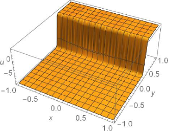
In this section, some numerical experiments are presented to illustrate the efficiency of our new approach. For each example, we first solve the forward problem, where we are looking for a solution to equation (1) in the form of an autowave, the existence and uniqueness of which is guaranteed by Theorem 3.1. Under Assumptions 1–4, the asymptotic solution to problem (1) has the following form:
| (109) |
where and are the solutions to the reduced equations (23) and (24).
To satisfy Assumption 4, we take the initial function in (1) as follows:
| (110) |
with an inner transition layer in the vicinity of .
For the simulation of inverse problems (IP) for determining the source function , we first solve the forward problem numerically using the finite-volume method, where we introduce the mesh uniformly with respect to spatial variables .
In the examples, we consider the case in which only measurements are provided, as a more complex scenario. We take the data obtained from the numerical result for the forward problem (Fig. 2) which belongs to the mesh knots and .
We skip the points from transition layer , and use nodes in only two regions, located on two sides of the transition layer, with indices , , and . The uniform noise (111) is added to the values to generate the artificial noisy data on the left and right intervals with respect to the transition layer:
| (111) |
where “rand” returns a pseudo-random value drawn from a uniform distribution on .
Following Algorithm 1, we obtain the smoothed data in accordance with optimization problems (65) and (66), for the left and right segments, respectively.
Finally, we calculate the regularized approximate source function using formula (64); the retrieved source function is then compared with the exact source function .
5.1 Example 1
5.1.1 Forward problem
Consider the following reaction–diffusion–advection equation in a two-dimensional setting with a periodic boundary condition along the axis and with the given source function :
| (112) |
We explicitly find the zero-order outer asymptotic functions:
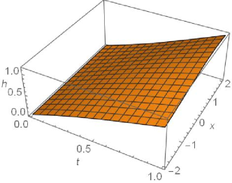
From the numerical solution to (33), we determine that the transition layer is located within the region for any (see Fig. 1); thus, Assumption 3 is satisfied.
According to (110), the initial function for problem (112) which satisfies Assumption 4 takes the form
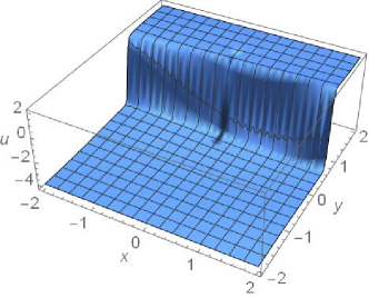
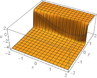
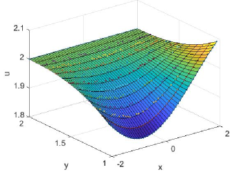
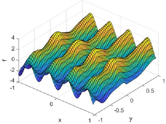
Thus, all the assumptions formulated in this paper are satisfied, and the solution to considered equation (112) is in the form of an autowave with a transitional moving layer localized near . The solution with the asymptotic expansion method for and in the zero approximation has the form (109), and is shown for in Fig. 2.
We also draw the numerical solution (using the finite-volume method) to problem (112) at the moment on Fig. 2, which we will use for the problem of identifying the source function.
The relative error of the asymptotic solution is
5.1.2 Inverse problem
We now consider the problem of identifying the source function in problem (112).
We use the following parameters: , , , , , .
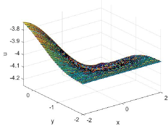
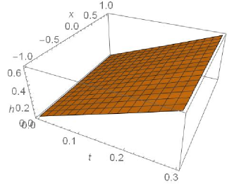
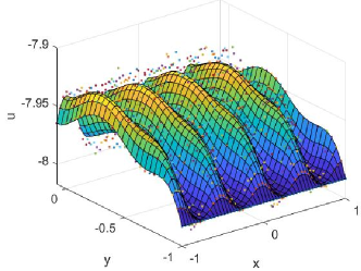
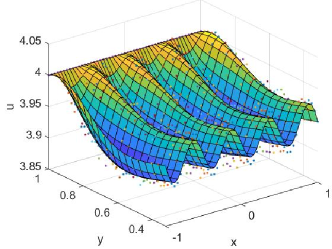
We take the data obtained from the forward problem with the numerical method on the regions and , and add random Gaussian noise with noise level to produce noisy data. Then, we smooth the obtained artificial noisy data on both intervals and obtain the smooth function (see Fig. 3).
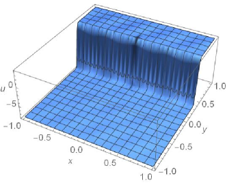
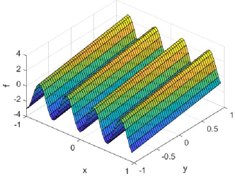
Following Algorithm 1, the regularized approximate source function calculated using formula (64) is drawn in Fig. 4.
The relative error of the recovered source function is , from which we can conclude that our approach is stable and accurate.

5.2 Example 2
5.2.1 Forward problem
We consider equation (112) with another source function and a periodic boundary condition along the axis:
| (113) |
The zero-order asymptotic outer functions have the following form:
The transition layer is located within the region for any (see Fig. 5), and thus Assumption 3 is satisfied. The initial function for problem (113), which satisfies Assumption 4, takes the form
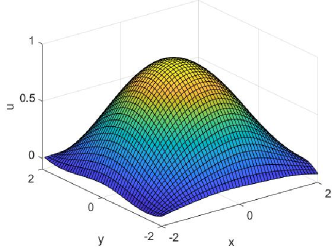
Thus, all the assumptions are satisfied and the considered equation, (113), has a solution in the form of an autowave; we represent the solution with the asymptotic expansion method (109) for in Fig. 6 and the numerical solution in Fig. 6 (which we will use for the problem of identifying the source function).
The relative error of the asymptotic solution is .
5.2.2 Inverse problem
We now consider the problem of identifying the source function of problem (113). The following parameters are used in the simulation: , , , , , .
Solving the inverse problem according to Algorithm 1 for the artificial noisy data obtained from the forward problem (113), we obtain the smooth function (see Fig. 7). According to Algorithm 1, the regularized approximate source function is calculated using formula (64); it is drawn in Fig. 8.
The relative error of the recovered source function is
6 Conclusion
In this paper, we develop an asymptotic expansion-regularization method for solving inverse source problems for two-dimensional time-dependent singularly perturbed PDEs. The essential idea is to use the asymptotic expansion methods to find a link equation between an unknown source function and the measurable quantities. By using the explored link equation, we avoid having to solve the PDE-constrained control problem. This simplification makes our inversion algorithm very efficient, and the methodology developed here can potentially be applied to a wide class of inverse problems in singularly perturbed PDEs.
Acknowledgments
This work was funded by the National Natural Science Foundation of China (No. 12171036), Beijing Natural Science Foundation (Key project No. Z210001), Guangdong Fundamental and Applied Research Fund (No. 2019A1515110971) and Shenzhen National Science Foundation (No. 20200827173701001).
References
- [1] M. Liberman, M. Ivanov, O. Peil, D. Valiev, L. Eriksson, Numerical studies of curved stationary flames in wide tubes, Combustion Theory and Modelling 7 (2003) 653–676.
- [2] O. Rudenko, Inhomogeneous burgers equation with modular nonlinearity: Excitation and evolution of high-intensity waves, Doklady Mathematics 95 (2017) 291–294.
- [3] V. Isakov, Inverse Source Problems, American Mathematical Society, New York, 1990.
- [4] R. Patterson, W. Wagner, A stochastic weighted particle method for coagulation-advection problems, SIAM Journal on Scientific Computing 34 (2012) 290–311.
- [5] H. Do, A. Owida, W. Yang, Y. Morst, Numerical simulation of the haemodynamics in end-to-side anastomoses, International Journal for Numerical Methods in Fluids 67 (2011) 638–650.
- [6] T. Bodnar, A. Sequeira, Numerical simulation of the coagulation dynamics of blood, Computational and Mathematical Methods in Medicine 9 (2008) 83–104.
- [7] A. Hidalgo, L. Tello, E. Toro, Numerical and analytical study of an atherosclerosis in ammatory disease model, Journal of Mathematical Biology 68 (2014) 1785–1814.
- [8] J. Berryman, C. Holland, Nonlinear diffusion problems arising in plasma physics, Physical Review Letters 40 (1978) 1720–1722.
- [9] Y. Zhang, G. Lin, P. Forssén, M. Gulliksson, T. Fornstedt, X. Cheng, A regularization method for the reconstruction of adsorption isotherms in liquid chromatography, Inverse Problem 32 (10) (2016) 105005.
- [10] Y. Zhang, G. Lin, M. Gulliksson, P. Forssén, T. Fornstedt, X. Cheng, An adjoint method in inverse problems of chromatography, Inverse Problems in Science and Engineering 25 (8) (2017) 1112–1137.
- [11] G. Lin, Y. Zhang, X. Cheng, M. Gulliksson, P. Forssén, T. Fornstedt, A regularizing Kohn-Vogelius formulation for the model-free adsorption isotherm estimation problem in chromatography, Applicable Analysis 97 (2018) 13–40.
- [12] X. Cheng, G. Lin, Y. Zhang, R. Gong, M. Gulliksson, A modified coupled complex boundary method for an inverse chromatography problem, Journal of Inverse and Ill-Posed Problems 26 (2018) 33–49.
- [13] C. Koudella, Z. Neufeld, Reaction front propagation in a turbulent flow, Physical Review E 70 (2004).
- [14] I. Amirkhanov, E. Zemlyanaya, I. Puzynin, T. Puzynina, N. Sarkar, I. Sarkhadov, Numerical simulation of evaporation of metals under the action of pulsed ion beams, Crystallography Reports 49 (2004) S123–S128.
- [15] C. Cosner, Reaction-diffusion-advection models for the effects and evolution of dispersal, Discrete and Continuous Dynamical Systems 34 (5) (2014) 1701–1745.
- [16] N. Vladimirova, V. Weirs, L. Ryzhik, Flame capturing with an advection–reaction–diffusion model, Combustion Theory and Modelling 10 (2006) 727 – 747.
- [17] A. Calder, D. Townsley, I. Seitenzahl, F. Peng, O. E. B. Messer, N. Vladimirova, E. Brown, J. Truran, D. Lamb, Capturing the fire : Flame energetics and neutronization for type ia supernova simulations, The Astrophysical Journal 656 (2007) 313–332.
- [18] M. Liberman, M. Ivanov, O. Peil, D. Valiev, L.-E. Eriksson, Numerical studies of curved stationary flames in wide tubes, Combustion Theory and Modelling 7 (2003) 653–676.
- [19] J. Burger, B. Sahuquet, Chemical aspects of in-situ combustion—heat of combustion and kinetics, Soc. Pet. Eng. J. 410 (01 1972).
- [20] J. Burger, Chemical aspects of in-situ combustion - heat of combustion and kinetics, Society of Petroleum Engineers Journal 12 (2013) 410–422.
- [21] N. Levashova, A. Sidorova, A. Semina, M. Ni, A spatio-temporal autowave model of shanghai territory development, Sustainability 11 (2019) 3658.
- [22] N. Nefedov, L. Recke, K. Schneider, Existence and asymptotic stability of periodic solutions with an interior layer of reaction–advection–diffusion equations, Journal of Mathematical Analysis and Applications 405 (1) (2013) 90–103.
- [23] E. Antipov, N. Levashova, N. Nefedov, Asymptotics of the front motion in the reaction-diffusion-advection problem, Computational Mathematics and Mathematical Physics 54 (2014) 1536–1549.
- [24] N. Levashova, N. Nefedov, O. Nikolaeva, Solution with an inner transition layer of a two-dimensional boundary value reaction-diffusion-advection problem with discontinuous reaction and advection terms, Theoretical and Mathematical Physics 207 (2021) 655–669.
- [25] E. Antipov, N. Levashova, N. Nefedov, Asymptotic approximation of the solution of the reaction-diffusion-advection equation with a nonlinear advective term, Modelirovanie i Analiz Informatsionnykh Sistem 25 (2018) 18–32.
- [26] E. Antipov, V. Volkov, N. Levashova, N. Nefedov, Moving front solution of the reaction-diffusion problem, Modelirovanie i Analiz Informatsionnykh Sistem 24 (2017) 259–279.
- [27] N. Nefedov, E. Nikulin, A. Orlov, On a periodic inner layer in the reaction-diffusion problem with a modular cubic source, Computational Mathematics and Mathematical Physics 60 (2020) 1461–1479.
- [28] V. Butuzov, A. Vasileva, M. Fedoryuk, Asymptotic methods in the theory of ordinary differential equations (in russian), Progress in Mathematics 8 (1970) 1–82.
- [29] N. Nefedov, An asymptotic method of differential inequalities for the investigation of periodic contrast structures: Existence, asymptotics, and stability, Differential Equations 36 (2000) 298–305.
- [30] N. Nefedov, Spike-type contrast structures in reaction-diffusion systems, Journal of Mathematical Sciences 150 (2008) 2540–2549.
- [31] D. Lukyanenko, V. Volkov, N. Nefedov, L. Recke, K. Schneider, Analytic-numerical approach to solving singularly perturbed parabolic equations with the use of dynamic adapted meshes, Modeling and Analysis of Information Systems 23 (2016) 334–341.
- [32] D. Lukyanenko, V. Volkov, N. Nefedov, Dynamically adapted mesh construction for the efficient numerical solution of a singular perturbed reaction-diffusion-advection equation, Modeling and Analysis of Information Systems 24 (2017) 322–338.
- [33] D. Lukyanenko, M. Shishlenin, V. Volkov, Solving of the coefficient inverse problems for a nonlinear singularly perturbed reaction-diffusion-advection equation with the final time data, Communications in Nonlinear Science and Numerical Simulation 54 (06 2017).
- [34] D. Lukyanenko, V. Grigorev, V. Volkov, M. Shishlenin, Solving of the coefficient inverse problem for a nonlinear singularly perturbed two-dimensional reaction–diffusion equation with the location of moving front data, Computers & Mathematics with Applications 77 (11 2018).
- [35] V. Volkov, N. Nefedov, Asymptotic solution of coefficient inverse problems for Burgers-type equations, Computational Mathematics and Mathematical Physics 60 (2020) 950–959.
- [36] A. Vasil’eva, V. Butuzov, N. Nefedov, Contrast structures in singularly perturbed problems, Fundamental and Applied Mathematics 4 (3) (1998) 799–851.
- [37] V. Butuzov, A. B. Vasil’eva, N. Nefedov, Asymptotic theory of contrast structures, Automation and Remote Control 58 (1997) 1068–1091.
- [38] Y. Wang, T. Wei, Numerical differentiation for two-dimensional scattered data, Journal of Mathematical Analysis and Applications 312 (1) (2005) 121–137.
- [39] N. Nefedov, The method of differential inequalities for some classes of nonlinear singularly perturbed problems with internal layers, Differential Equations 31 (1995) 1142–1149.
- [40] D. Sattinger, Monotone methods in elliptic and parabolic boundary value problems, Indiana University Mathematics Journal 21 (1972) 979–1001.
- [41] C. Pao, Nonlinear Parabolic and Elliptic Equations, Plenum Press, New York, London, 1992.