Robust Estimation and Inference
in Panels with Interactive Fixed Effects

Abstract

We consider estimation and inference for a regression coefficient in panels with interactive fixed effects (i.e., with a factor structure). We show that previously developed estimators and confidence intervals (CIs) might be heavily biased and size-distorted when some of the factors are weak. We propose estimators with improved rates of convergence and bias-aware CIs that are uniformly valid regardless of whether the factors are strong or not. Our approach applies the theory of minimax linear estimation to form a debiased estimate using a nuclear norm bound on the error of an initial estimate of the interactive fixed effects. We use the obtained estimate to construct a bias-aware CI taking into account the remaining bias due to weak factors. In Monte Carlo experiments, we find a substantial improvement over conventional approaches when factors are weak, with little cost to estimation error when factors are strong.

1 Introduction

In this paper, we consider a linear panel regression model of the form

$$Y_{it}=X_{it}\beta+\sum_{k=1}^{K}Z_{k,it}\delta_{k}+\Gamma_{it}+U_{it},$$ (1)

where $Y_{it},X_{it},Z_{1,it},\ldots,Z_{K,it}\in\mathbb{R}$ are the observed outcome variable and covariates for units $i=1,\ldots,N$ and time periods $t=1,\ldots,T$. The error components $\Gamma_{it}\in\mathbb{R}$ and $U_{it}\in\mathbb{R}$ are unobserved, and the regression coefficients $\beta,\delta_{1},\ldots,\delta_{K}\in\mathbb{R}$ are unknown. The parameter of interest is $\beta\in\mathbb{R}$, the coefficient on $X_{it}$. We are interested in “large panels”, where both $N$ and $T$ are relatively large.

The error component $U_{it}$ is modelled as a mean-zero random shock that is uncorrelated with the regressors $X_{it}$ and $Z_{k,it}$ and that is at most weakly autocorrelated across $i$ and over $t$. By contrast, the error component $\Gamma_{it}$ can be correlated with $X_{it}$ and $Z_{k,it}$ and can also be strongly autocorrelated across $i$ and over $t$. Of course, further restrictions on $\Gamma_{it}$ are required to allow estimation and inference on $\beta$. For example, the additive fixed effect model imposes that $\Gamma_{it}=\alpha_{i}+\gamma_{t}$, where $\alpha_{i}$ accounts for any omitted variable that is constant over time, and $\gamma_{t}$ for any omitted variable that is constant across units. Instead of this additive fixed effect model we will mostly consider the so-called interactive fixed effect model, where

$$\Gamma_{it}=\sum_{r=1}^{R}\,\lambda_{ir}\,f_{tr}\;.$$ (2)

Here, the $\lambda_{ir}$ and $f_{tr}$ can either be interpreted as unknown parameters or as unobserved shocks. This model for $\Gamma_{it}$ is also referred to as a factor model with factors loadings $\lambda_{ir}$ and factors $f_{tr}$, and we will use the factor and interactive fixed effect terminology synonymously. The number of factors $R$ is unknown, but is assumed to be small relative to $N$ and $T$. The interactive fixed effect model is attractive because it introduces enough restrictions to allow estimation and inference on $\beta$ while still incorporating or approximating a large class of data generating processes (DGPs) for $\Gamma_{it}$.

The existing econometrics literature on panel regressions with interactive fixed effects is quite large. Since the seminal work of Pesaran (2006) and Bai (2009), developing tools for estimation and inference on $\beta$ in model (1)-(2) under large $N$ and large $T$ asymptotics has been a primary focus of this literature. Specifically, Pesaran (2006) introduces the common correlated effects (CCE) estimator, which uses cross-sectional averages of the observed variables as proxies for the unobserved factors. Bai (2009) derives the large $N$, $T$ properties of the least-squares (LS) estimator that jointly minimizes the sum of squared residuals over the regression coefficients, factors, and factor loadings.

Bai (2009) shows that, under appropriate assumptions, the LS estimator for the regression coefficients is $\sqrt{NT}$-consistent and asymptotically normally distributed as both $N$ and $T$ grow to infinity. One of the key assumptions imposed for this result is the so-called “strong factor assumption”, which requires all the factor loadings $\lambda_{ir}$ and factors $f_{tr}$ to have sufficient variation across $i$ and over $t$, respectively. If the strong factor assumption is violated, then the LS estimator for $\lambda_{ir}$ and $f_{tr}$ may be unable to pick up the true loadings and factors correctly, because the “weak factors” in $\Gamma_{it}$ cannot be distinguished from the noise in $U_{it}$. This can lead to substantial bias and misleading inference, due to omitted variables bias from $\Gamma_{it}$ that is not picked up by the estimator.

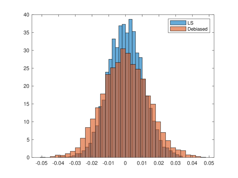
(a) No ID ($\kappa=0.00$)

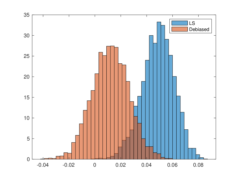
(b) Weak ID ($\kappa=0.10$)

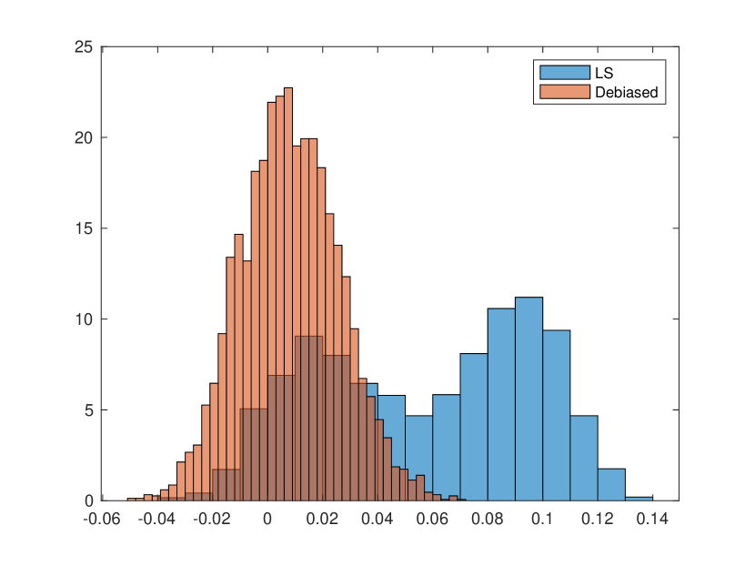
(c) Weak ID ($\kappa=0.20$)

(d) Strong ID ($\kappa=1.00$)

Figure 1: Finite sample distributions of the LS and the debiased estimators, $N=100$, $T=50$, $R=1$

To illustrate how this can lead to problems with conventional estimates and CIs for $\beta$, Figure 1 presents a subset of the results of our Monte Carlo study. When the factors are nonexistent (panel a) or strongly identified (panel d), the distribution of the LS estimator (in blue) is centered at the true parameter value $\beta$ (equal to $0$ in this case). However, when the factors are present but weak enough that they are difficult to detect (panels b and c), the LS estimator is heavily biased and non-normally distributed. In our Monte Carlo study in Section 5, we show that this indeed leads to severe coverage distortion, with conventional CIs based on the LS estimator having almost zero coverage.

In this paper, we address this issue by developing new tools for estimation and inference on $\beta$ in the model (1). We develop a debiased estimator along with a bound on the remaining bias, which we use to construct a bias-aware confidence interval. As illustrated in Figure 1, our debiased estimator (shown in red) substantially decreases the bias of the LS estimator when factors are weak, leading to a large improvement in overall estimation error. In addition, this improved performance under weak factors does not come at a substantial cost to performance when factors are strong or nonexistent: our debiased estimator performs similarly to the LS estimator in these cases. Importantly, our CI requires only an upper bound on the number of factors: we show that it is valid uniformly over a large class of DGPs that allows for weak, strong or nonexistent factors up to a specified upper bound on the number of factors. We derive rates of convergence that hold uniformly over this class of DGPs, and we show that our estimator achieves a faster uniform rate of convergence than existing approaches when weak factors are allowed. In the case where $N$ and $T$ grow at the same rate, our estimator achieves the parametric $\sqrt{NT}$ rate.

Our debiasing approach uses a preliminary estimate $\hat{\Gamma}_{\rm pre}$ of the individual effect matrix $\Gamma$ along with a bound $\hat{C}$ on the nuclear norm $\|\Gamma-\hat{\Gamma}_{\rm pre}\|_{*}$ of its estimation error. Letting $\tilde{\Gamma}:=\Gamma-\hat{\Gamma}_{\rm pre}$, we then consider the augmented outcomes

$$\tilde{Y}_{it}:=Y_{it}-\hat{\Gamma}_{{\rm pre},it}=X_{it}\beta+\sum_{k=1}^{K}Z_{k,it}\delta_{k}+\tilde{\Gamma}_{it}+U_{it}.$$

Treating $\tilde{\Gamma}_{it}$ as nuisance parameters satisfying a convex constraint $\|\tilde{\Gamma}\|_{*}\leq\hat{C}$, we derive linear weights $A_{it}$ such that the estimator $\sum_{i=1}^{N}\sum_{t=1}^{T}A_{it}\tilde{Y}_{it}$ for $\beta$ optimally uses this constraint, using the theory of minimax linear estimators (see Ibragimov and Khas’minskii, 1985; Donoho, 1994; Armstrong and Kolesár, 2018). In particular, the resulting weights $A_{it}$ control the remaining omitted variables bias $\sum_{i=1}^{N}\sum_{t=1}^{T}A_{it}\tilde{\Gamma}_{it}$ due to possible weak factors in $\tilde{\Gamma}=\Gamma-\hat{\Gamma}_{\rm pre}$ not picked up by the initial estimate $\hat{\Gamma}_{\rm pre}$.

A key step in deriving our CI is the construction of the preliminary estimator $\hat{\Gamma}_{\rm pre}$ and bound $\hat{C}$ on the nuclear norm of its estimation error. Our CI is bias-aware: it uses the bound $\hat{C}$ to explicitly take into account any remaining bias in the debiased estimator. Our bound is feasible once an upper bound on the number of factors is specified. In our Monte Carlo study, we find that, while our CIs are often conservative, they are about as wide as an “oracle” CI that uses an infeasible critical value to correct the coverage of a CI based on the standard LS estimator.

Although the main focus of this paper is on models with the pure factor structure (2), the proposed approach applies to general interactive fixed effects models as long as it is possible to construct an upper bound on $\|\tilde{\Gamma}\|_{*}$. In particular, the proposed approach naturally extends to settings with nonseparable interactive unobserved heterogeneity (e.g., Zeleneev, 2019; Fernández-Val, Freeman and Weidner, 2021; Freeman and Weidner, 2021), for which, to the best of our knowledge, no tools for inference were previously available. Our approach also allows relaxing the strong group separation assumption in models with grouped unobserved heterogeneity (e.g., Assumption 2(b) in Bonhomme and Manresa, 2015), which is analogous in spirit to the “strong factor assumption”. This is practically appealing because, unlike existing approaches, our method allows overspecifying the true number of groups, which in addition could be weakly separated.

Finally, rather than imposing the factor model (1), one may wish to impose an a priori bound on the nuclear norm $\|\Gamma\|_{*}$ of the individual effects matrix directly. In this case, our approach applies with the initial estimate $\hat{\Gamma}_{\rm pre}$ set to zero, which leads to a direct application of minimax linear estimators as in Donoho (1994) and Armstrong and Kolesár (2018). More generally, our approach can be extended to other panel settings with matrix restrictions, such as introducing heterogeneous coefficients $\beta_{it}$ for each $X_{it}$ and placing rank or nuclear norm restrictions on the matrix of these coefficients (as in Athey, Bayati, Doudchenko, Imbens and Khosravi, 2021). The main requirement is the availability of a convex bound on matrices that enter the regression model, or on the error of an initial estimate of such matrices.

Related literature

There exist various alternative estimation methods for panel regressions with interactive fixed effects. For example, Holtz-Eakin, Newey and Rosen (1988) introduce the the quasi-difference approach, Ahn, Lee and Schmidt (2001, 2013) use generalized method of moments estimation, and Chamberlain and Moreira (2009) use invariance arguments to derive procedures that satisfy a Bayes-minimax property. All those papers assume fixed $T$, with only $N$ going to infinity. More recent papers investigating the fixed $T$ large $N$ case include Robertson and Sarafidis (2015), Juodis and Sarafidis (2018), Westerlund, Petrova and Norkute (2019), Higgins (2021), Juodis and Sarafidis (2022). As mentioned before, in the context of large $N$ and large $T$ panels, two seminal works that have spurred a very large number of follow-up papers are Pesaran (2006) and Bai (2009) — for a review and further references see Bai and Wang (2016). A special case of the violation of the strong factor assumption is when some factor are equal to zero, while all other factors are strong; the inference results of Bai (2009) are usually robust towards this specific violation of the strong factor assumption (Moon and Weidner, 2015). This robustness, however, does not carry over to more general weak factors in the DGP of $\Gamma_{it}$, as illustrated by Figure 1.

The problem of weak factors is related to the problem of omitted variable bias of LASSO estimators in high dimensional regression that is the focus of debiased LASSO estimators (see Belloni, Chernozhukov and Hansen, 2014; Javanmard and Montanari, 2014; van de Geer, Bühlmann, Ritov and Dezeure, 2014; Zhang and Zhang, 2014). Just as LASSO estimators omit variables with coefficients that are large enough to cause omitted variables bias but too small to distinguish from zero, weak factors in $\Gamma$ can be difficult to detect, leading to omitted variables bias in conventional estimates of $\beta$. Our approach to using minimax linear estimation to debias an initial estimate mirrors the approach of Javanmard and Montanari (2014) to debiasing the LASSO. We discuss this connection further in Section 4.3. Hirshberg and Wager (2020) provide a general discussion and further references for minimax linear debiasing; we refer to this general approach as augmented linear estimation following their terminology. Minimax linear estimation itself goes back at least to Ibragimov and Khas’minskii (1985), with further results on this approach and its optimality properties in Donoho (1994), Armstrong and Kolesár (2018) and Yata (2021), among others. The particular form of the minimax estimator used for debiasing in our setup follows from a formula given in Armstrong, Kolesár and Kwon (2020).

Requiring $\Gamma_{it}$ to have the factor structure (2) is equivalent to requiring the matrix of unobserved effects $\Gamma$ to have rank at most $R$, i.e., having ${\rm rank}(\Gamma)\leq R$. Bounding the nuclear norm of $\tilde{\Gamma}$ or $\Gamma$ instead can also be seen as a convex relaxation of this requirement. Similar convexifications of the rank constraint have been widely used in the matrix completion literature (e.g., Recht, Fazel and Parrilo 2010 and Hastie, Tibshirani and Wainwright 2015 for recent surveys), and for reduced rank regression estimation (e.g., Rohde and Tsybakov 2011). In the econometrics literature, the numerous applications of this idea include, for example, estimation of pure factor models (Bai and Ng, 2017), estimation of panel regression models with homogeneous (Moon and Weidner, 2018; Beyhum and Gautier, 2019) and heterogeneous coefficients (Chernozhukov, Hansen, Liao and Zhu, 2019), estimation of treatment effects (Athey, Bayati, Doudchenko, Imbens and Khosravi, 2021; Fernández-Val, Freeman and Weidner, 2021), and many others. However, none of these papers obtain asymptotically valid CIs or improved rates of convergence under weak factors.

In recent work, Chetverikov and Manresa (2022) propose an estimator that, like ours, achieves a faster rate of convergence than conventional approaches under weak factors. While Chetverikov and Manresa (2022) allow for weak factors in some of their estimation results, they assume strong factors when constructing CIs. The estimation approach in Chetverikov and Manresa (2022) also differs from our approach by using modelling assumptions that place a factor structure on the covariate matrix $X$.

Our focus is on allowing for weak factors without imposing additional assumptions on the error term $U$, such as homoskedasticity or full independence from the individual effects $\Gamma$ and regressor $X$. Such additional structure allows for further identifying information by making it easier to distinguish between the error term $U$ and the individual effects $\Gamma$, leading to a fundamentally different analysis. Zhu (2019) derives asymptotic upper and lower bounds for estimators and CIs in a setting with possible weak factors under homoskedastic and fully independent errors. The estimators and CIs constructed by Zhu (2019) take advantage of the additional structure of Zhu’s setting, making them inapplicable in ours. However, the lower bounds derived by Zhu (2019) are immediately relevant: they show that no CI can be asymptotically valid under weak factors while mimicking the performance of the CI of Bai (2009) when factors are strong.

Beyhum and Gautier (2022), Fan and Liao (2022), and Bai and Ng (2023) consider estimation and inference in various settings under a regime in which a lower bound on the strength of the factors can decrease with $N$ and $T$, but is large enough that factors can be consistently estimated. This is analogous to the “semi-strong” regime in weak instrument and related settings; see Andrews and Cheng (2012). While the semi-strong regime requires careful theoretical analysis, the fact that factors can be consistently estimated leads to asymptotically unbiased and normal estimators for the main effect $\beta$. Our results apply to semi-strong and strong regimes as well, while also allowing for weak factor regimes in which factors cannot be consistently estimated.

Finally, Cox (2022) develops tools for inference in low-dimensional factor models with weak identification. In Cox (2022), the primary objects of interests are the covariance of the factors and the loadings. The baseline model in Cox (2022) does not include observed covariates, whereas we focus on estimation and inference on $\beta$, the coefficient on $X_{it}$, exclusively.

The rest of this paper is organized as follows. Section 2 introduces the framework and describes construction of the debiased estimator and bias-aware CI. Section 3 provides additional implementation details for the factor model. Section 4 provides formal statistical guarantees. Section 5 considers numerical and empirical illustrations. Appendix A contains proofs of the results in the main text. Appendix B provides additional computational details. Appendices C and D contain additional results for the numerical and empirical illustrations.

2 Construction of robust estimates and confidence intervals

2.1 Setup

We consider a panel setting in which we observe a scalar outcome $Y_{it}$, a scalar covariate $X_{it}$ of interest and additional control covariates $\{Z_{k,it}\}_{k=1}^{K}$ for $i=1,\ldots,N$, $t=1,\ldots,T$, which follow the regression model (1). The error term $U_{it}$ is assumed to be mean zero conditional on $X$, $\{Z_{k,it}\}_{k=1}^{K}$ and $\Gamma$, but we allow for heteroskedasticity, which may depend on $X_{it}$ and $\Gamma_{it}$, as well as some weak dependence. We write the model in matrix notation as

$$Y=X\beta+Z\cdot\delta+\Gamma+U\,,\qquad\qquad\mathbb{E}[U|X,Z,\Gamma]=0\,,$$ (3)

where $Z$ denotes the three dimensional array $\{Z_{k,it}\}$ and we define $Z\cdot\delta=\sum_{k=1}^{K}Z_{k}\delta_{k}$ where $Z_{k}$ denotes the matrix with $i,t$-th element $Z_{k,it}$.

We are interested in the coefficient $\beta$ of $X_{it}$, which can be interpreted as the effect of a treatment variable $X_{it}$ in a constant treatment effects model (we discuss extensions to heterogeneous treatment effects in Remark 2.3). For concreteness, we use panel notation, and we refer to $i$ and $t$ as individuals and time periods respectively. However, we allow for other settings such as network data in which $i$ and $t$ both index individuals in a network. While we will assume a low rank structure on $\Gamma$, we allow for arbitrary dependence between the covariate $X_{it}$ and the individual effect $\Gamma_{it}$.

To apply our approach, we require a bound on the nuclear norm of the difference $\Gamma-\hat{\Gamma}$ for some preliminary estimate $\hat{\Gamma}$ of the matrix $\Gamma$:

$$\big{\|}\widetilde{\Gamma}\big{\|}_{*}\leq\hat{C}\,,\qquad\text{where}\qquad\widetilde{\Gamma}:=\Gamma-\hat{\Gamma}\,.$$ (4)

Here, $\|\cdot\|_{*}$ denotes the nuclear norm of the argument matrix, and $\hat{C}\geq 0$ is a known or estimated constant. We focus on two main cases where such bounds are available.

Case 1.

$\hat{\Gamma}\neq 0$ and $\hat{C}$ is estimated from the data. This is the case that is practically most relevant in this paper, where $\hat{\Gamma}$ is estimated such that a relatively small value for $\hat{C}$ can be chosen. To obtain $\hat{\Gamma}$ and $\hat{C}$ we will later assume that $\Gamma$ has a linear factor structure with at most $R$ factors.

Case 2.

$\hat{\Gamma}=0$ and $\hat{C}$ is a known constant. In this case we have $\widetilde{\Gamma}=\Gamma$ and the bound $\hat{C}$ constitutes an a priori bound on the nuclear norm of $\Gamma$. While this case is less practically relevant to this paper, it provides for an idealized setting that motivates some of our arguments later in this section.

2.2 (Augmented) linear estimators and CIs

We first define a class of estimators and CIs, indexed by an $N\times T$ matrix $A$. We then provide a choice of the matrix $A$, based on finite sample optimality in an idealized setting. Our class of estimators is given in the following definition.

Definition 2.1.

Let $A=A(X,Z)$ be an $N\times T$ matrix of weights $A_{it}\in\mathbb{R}$ that can depend on the matrix $X$ and array $Z$. Let $\hat{\Gamma}$ be an initial estimate of $\Gamma$, and let $\widetilde{Y}=Y-\hat{\Gamma}$. The augmented linear estimator with weight matrix $A$ and initial estimate $\hat{\Gamma}$ is given by

$$\hat{\beta}_{A} :=\sum_{i=1}^{N}\sum_{t=1}^{T}A_{it}\widetilde{Y}_{it}=\langle A,\widetilde{Y}\rangle_{F}.$$ (5)

Here, $\langle\cdot,\cdot\rangle_{F}$ denotes the entry-wise inner product between between the argument matrices.

Remark 2.1.

In Case 2, $\widetilde{Y}=Y$ so that $\hat{\beta}_{A}$ is a linear estimator in the classical sense: it is linear in the outcomes $Y_{it}$, with weights depending on the design points $X_{it},Z_{1,it},\ldots,Z_{k,it}$. In Case 1, the estimator $\hat{\beta}_{A}=\langle A,\widetilde{Y}\rangle_{F}$ applies a linear estimator after an initial estimation step in which the initial estimate $\hat{\Gamma}$ is subtracted from the outcome $Y$. This mirrors applications of this idea in other settings going back to Javanmard and Montanari (2014); see Hirshberg and Wager (2020) for references (the term “augmented linear estimation” is used in the latter paper).

To analyze this class of estimators, note that subtracting the initial estimate from both sides of the equation (3) gives

$$\widetilde{Y}=X\beta+Z\cdot\delta+\widetilde{\Gamma}+U$$ (6)

(recall that $\widetilde{Y}=Y-\hat{\Gamma}$ and $\widetilde{\Gamma}=\Gamma-\hat{\Gamma}$). This gives the decomposition

$$\hat{\beta}_{A}-\beta=\operatorname{bias}_{\beta,\delta,\widetilde{\Gamma}}(\hat{\beta}_{A})+\langle A,U\rangle_{F}$$ (7)

where

$$\operatorname{bias}_{\beta,\delta,\widetilde{\Gamma}}(\hat{\beta}_{A}):=\left(\langle A,X\rangle_{F}-1\right)\beta+\langle A,Z\cdot\delta\rangle_{F}+\langle A,\widetilde{\Gamma}\rangle_{F}.$$ (8)

In Case 2, we have $\Gamma=\widetilde{\Gamma}$ and $\operatorname{bias}_{\beta,\delta,\Gamma}(\hat{\beta}_{A})=E[\hat{\beta}_{A}-\beta|X,Z,\Gamma]$ gives the bias of $\hat{\beta}_{A}$ conditional on $X,Z$ and $\Gamma$. In Case 1, $\operatorname{bias}_{\beta,\delta,\widetilde{\Gamma}}$ does not literally give the bias or conditional bias of $\hat{\beta}_{A}$, since conditioning on $\widetilde{\Gamma}=\Gamma-\hat{\Gamma}$ means conditioning on an information set that depends on $Y$ through the preliminary estimate $\hat{\Gamma}$. We nonetheless refer to $\operatorname{bias}_{\beta,\delta,\Gamma}(\hat{\beta}_{A})$ as a bias term, in analogy to Case 2.

Let $\widehat{\operatorname{se}}$ be an estimate of the standard deviation of $\langle A,U\rangle_{F}=\sum_{i=1}^{N}\sum_{t=1}^{T}A_{it}U_{it}$. For example, to allow for arbitrary heteroskedasticity in $U_{it}$ while imposing independence across $i$ and $t$, we can use $\widehat{\operatorname{se}}=\sqrt{\sum_{i=1}^{N}\sum_{t=1}^{T}A_{it}^{2}\hat{U}_{it}^{2}}$ where $\hat{U}_{it}$ denotes residuals from an initial regression. If $\operatorname{bias}_{\beta,\delta,\Gamma}(\hat{\beta}_{A})$ were zero, then we could form a CI by adding and subtracting a normal critical value times $\widehat{\operatorname{se}}$. To take into account the possibility that $\operatorname{bias}_{\beta,\delta,\Gamma}(\hat{\beta}_{A})$ will in general be nonnegligible in our setting, we use the bound (4) to obtain an upper bound on the bias term. In particular, when (4) holds, we have $\left|\operatorname{bias}_{\beta,\delta,\widetilde{\Gamma}}(\hat{\beta}_{A})\right|\leq\overline{\operatorname{bias}}_{\hat{C}}(\hat{\beta}_{A})$, where for general $C\geq 0$ we define

$$\overline{\operatorname{bias}}_{C}(\hat{\beta}_{A}) :=\sup_{\beta,\delta,\widetilde{\Gamma}:\|\widetilde{\Gamma}\|_{*}\leq C}\operatorname{bias}_{\beta,\delta,\widetilde{\Gamma}}(\hat{\beta}_{A})$$

$$=\begin{cases}\displaystyle\sup_{\widetilde{\Gamma}:\|\widetilde{\Gamma}\|_{*}\leq C}\langle A,\widetilde{\Gamma}\rangle_{F}&\text{if}\,\langle A,X\rangle_{F}=1,\,\text{and }\langle A,Z_{k}\rangle_{F}=0,\,\text{for }k=1,\ldots K,\\ \infty&\text{otherwise}\end{cases}$$

$$=\begin{cases}Cs_{1}(A)&\text{if}\,\langle A,X\rangle_{F}=1,\,\text{and }\langle A,Z_{k}\rangle_{F}=0,\,\text{for }k=1,\ldots K,\\ \infty&\text{otherwise.}\end{cases}$$ (9)

Here, for the second equality we used that the supremum over $\beta$ and $\delta$ is unbounded unless $\langle A,X\rangle_{F}=1$ and $\langle A,Z_{k}\rangle_{F}=0$, and for the final step we used that the nuclear norm $\|\cdot\|_{*}$ is dual to the spectral norm, which we denote by $s_{1}(\cdot)$ since it is equal to the largest singular value of the argument matrix. We refer to $\overline{\operatorname{bias}}_{\hat{C}}(\hat{\beta}_{A})$ as the worst-case bias of the estimator $\hat{\beta}_{A}$ (again, this is only literally true in Case 2, but we use the same terminology in Case 1 by analogy).

Note that, whereas $\operatorname{bias}_{\beta,\delta,\widetilde{\Gamma}}(\hat{\beta}_{A})$ depends on the unknown matrix of individual effects $\Gamma$ through the matrix $\widetilde{\Gamma}=\Gamma-\hat{\Gamma}$, $\overline{\operatorname{bias}}_{\hat{C}}(\hat{\beta}_{A})$ is feasible to compute once a bound $\hat{C}$ is given. Taking into account the possible bias leads to a bias-aware CI:

$$\left\{\hat{\beta}_{A}\pm\left[\overline{\operatorname{bias}}_{\hat{C}}(\hat{\beta}_{A})+z_{1-\alpha/2}\widehat{\operatorname{se}}\right]\right\}.$$ (10)

To motivate this CI, note that the probability that the lower endpoint is greater than $\beta$ is

$$P\left(\hat{\beta}_{A}-\overline{\operatorname{bias}}_{\hat{C}}(\hat{\beta}_{A})-z_{1-\alpha/2}\widehat{\operatorname{se}}>\beta\right)=P\left(\sum_{i=1}^{N}\sum_{t=1}^{T}A_{it}U_{it}+\operatorname{bias}_{\beta,\delta,\widetilde{\Gamma}}(\hat{\beta}_{A})>\overline{\operatorname{bias}}_{\hat{C}}(\hat{\beta}_{A})+z_{1-\alpha/2}\widehat{\operatorname{se}}\right)$$

$$\leq P\left(\sum_{i=1}^{N}\sum_{t=1}^{T}A_{it}U_{it}>z_{1-\alpha/2}\widehat{\operatorname{se}}\right)\approx\alpha/2,$$

where the last step assumes that $\sum_{i=1}^{N}\sum_{t=1}^{T}A_{it}U_{it}$ is approximately normally distributed with zero mean and standard deviation close to $\widehat{\operatorname{se}}$. We provide formal justifications for this later. Combining this with similar calculations for undercoverage in the other direction shows that the coverage is approximately at least $1-\alpha$.

Remark 2.2.

In Case 2 where $\widetilde{\Gamma}=\Gamma$ is non-random, one can take advantage of the fact that $\operatorname{bias}_{\beta,\delta,\widetilde{\Gamma}}$ is non-random, which allows for the shorter CI $\left\{\hat{\beta}_{A}\pm\operatorname{cv}_{\alpha}\left(\overline{\operatorname{bias}}_{C}(\hat{\beta}_{A})/\widehat{\operatorname{se}}\right)\cdot\widehat{\operatorname{se}}\right\}$ where $\operatorname{cv}_{\alpha}(t)$ denotes the $1-\alpha$ quantile of the absolute value of a $N(t,1)$ random variable (see Donoho, 1994; Armstrong and Kolesár, 2018). In order to keep the exposition simple while covering both cases, we focus on the CI given in (10).

Remark 2.3.

In principle, our approach can be extended to a heterogeneous treatment effect model where the constant coefficient $\beta$ is replaced by an individual specific coefficient $\beta_{it}$ that is allowed to vary with $i$ and $t$. In particular, if a bound on the nuclear norm of the matrix of coefficients $\beta_{it}$ or on the error of preliminary estimates of these coefficients is available in addition to such a bound for $\Gamma$, we can use minimax linear debiasing to estimate a linear functional of the individual specific effects $\beta_{it}$. For example, the linear functional $\frac{1}{NT}\sum_{i=1}^{N}\sum_{t=1}^{T}\beta_{it}$ gives the average treatment effect of a one-unit change in $X_{it}$ over the $NT$ units in a setting where $\beta_{it}$ is interpreted as the causal effect of a change in the variable $X_{it}$. We leave such extensions as a topic for future research.

2.3 Choice of weights $A=(A_{it})$

As described in the last subsection, one can construct valid confidence intervals for $\beta$ of the form (10) for any choice of weight matrix $A$, subject to weak regularity conditions. To get a simple baseline procedure, we compute weights that are optimal in an idealized setting where $U_{it}\stackrel{{\scriptstyle iid}}{{\sim}}N(0,\sigma^{2})$. In Case 2, $\hat{\beta}_{A}$ is then normally distributed with variance $\sigma^{2}\sum_{i=1}^{N}\sum_{t=1}^{T}A_{it}^{2}=\sigma^{2}\|A\|_{F}^{2}$ (where $\|\cdot\|_{F}$ denotes the Frobenius norm), and with bias ranging from $-\overline{\operatorname{bias}}_{\hat{C}}(\hat{\beta}_{A})$ to $\overline{\operatorname{bias}}_{\hat{C}}(\hat{\beta}_{A})$. Thus, if we choose worst-case MSE under i.i.d. normal errors as our criterion function for the weights, then the optimal weights are obtained by minimizing $\left(\overline{\operatorname{bias}}_{\hat{C}}(\hat{\beta}_{A})\right)^{2}+\sigma^{2}\|A\|_{F}^{2}$. Plugging in the formula for $\overline{\operatorname{bias}}_{\hat{C}}(\hat{\beta}_{A})$ given in (9) gives the following baseline choice of weights, indexed by a tuning parameter ${b}$ that plays the role of $\hat{C}/\sigma$.

Definition 2.2.

For ${b}>0$, define the “optimal” $N\times T$ weight matrix by

$$A^{*}_{{b}} :=\operatorname*{argmin}_{A\in\mathbb{R}^{N\times T}}\,{b}^{2}s_{1}(A)^{2}+\|A\|_{F}^{2}\;\;\qquad\text{s.t.}\quad\text{$\langle A,X\rangle_{F}=1$ and $\langle A,Z_{k}\cdot\delta\rangle_{F}=0$,}$$

Here, the constraint $\langle A,Z_{k}\cdot\delta\rangle_{F}=0$ is imposed for all $k\in\{1,\ldots,K\}$.

The weights in Definition 2.2 are optimal in Case 2 when $\hat{C}/\sigma={b}$. Heuristically, we also expect that, in Case 1, a good choice of ${b}$ will correspond to $\hat{C}/\sigma$ such that the bound $\hat{C}$ on the nuclear norm holds with high probability. Conveniently, our nuclear norm bound in the exact factor model in Section 3 scales with the standard deviation $\sigma$ in the homoskedastic case, which gives us a simple and feasible choice of the tuning parameter ${b}$.

We emphasize again that while the definition of $A^{*}_{b}$ is motivated by the idealized setting $U_{it}\stackrel{{\scriptstyle iid}}{{\sim}}N(0,\sigma^{2})$, we do not assume that the error terms $U_{it}$ satisfy this strong assumption in this paper. Choosing $A=A^{*}_{b}$ to construct the estimator $\hat{\beta}_{A}$ and the confidence intervals (10) under more general error distributions just means that the resulting estimates and confidence intervals will not be optimal (in finite samples), but we will nevertheless show them to be consistent and valid, respectively.

Remark 2.4.

While we have used MSE to motivate our baseline choice of weights $A^{*}_{b}$, one could use other criteria corresponding to different weights on bias and variance. For example, optimizing CI length when $\hat{C}/\sigma=b$ would give the criterion ${b}s_{1}(A)+z_{1-\alpha}\|A\|_{F}$. If $\beta$ gives the net welfare gain of an all-or-nothing policy change, then one can target minimax welfare regret as in Ishihara and Kitagawa (2021) and Yata (2021). In our Monte Carlo simulations however, we find that the exact choice of criterion has little effect on performance.

2.4 Practical implementation

The definition of $A^{*}_{b}$ is a convex optimization problem that can easily be solved numerically for any given input $X$, $Z$, ${b}$. Using results from Armstrong, Kolesár and Kwon (2020), it follows that $A^{*}_{b}$ can also be computed using the residuals of a nuclear norm regularized regression of $X$ on $Z_{1},\ldots,Z_{K}$ and a matrix of individual effects. In the case with no additional covariates $Z$, this nuclear norm regularized regression simplifies further: it can be solved by computing the singular value decomposition of $X$, and then performing soft thresholding on the singular values. The resulting weights $A^{*}_{b}$ obtained from the residuals of this regression replace the largest singular values of $X$ with a constant. We provide details in Appendix B.

In addition to giving alternative methods for computing the weights $A^{*}_{b}$, these results provide some intuition for these weights. The residuals from this nuclear norm regularized regression of $X$ on $Z_{1},\ldots,Z_{K}$ and the individual effects “partial out” potential correlation of $X$ with the estimation error $\widetilde{\Gamma}$, similar to the estimator of Robinson (1988) in the partially linear model. In the case with no additional covariates $Z$, this amounts to removing the largest singular values of $X$ and replacing them with a constant.

To summarize, we can compute an estimator $\hat{\beta}_{A}$ using Definition 2.1 using any matrix of weights $A$. We can also compute a CI $\left\{\hat{\beta}_{A}\pm\left[\overline{\operatorname{bias}}_{\hat{C}}(\hat{\beta}_{A})+z_{1-\alpha/2}\widehat{\operatorname{se}}\right]\right\}$ as in (10), once we have a standard error $\widehat{\operatorname{se}}$ and an upper bound $\hat{C}$ for the nuclear norm of the error in the initial estimate of $\Gamma$. Definition 2.2 gives us a heuristic for computing a reasonable choice of the matrix $A$, once we have an initial choice of ${b}$ for the ratio $\hat{C}/\sigma$ of the nuclear norm bound to variance of $U_{it}$.

Thus, to apply our general approach with data $\tilde{Y},X,Z$ (with $\widetilde{Y}$ computed by subtracting an initial estimate of $\Gamma$ in Case 1), we need an initial choice ${b}$ to compute the weights $A^{*}_{b}$ using Definition 2.2. We also need a robust upper bound $\hat{C}$ such that the bound (4) holds with high probability. Finally, we need a robust standard error $\widehat{\operatorname{se}}$. Our CI then takes the form in (10) with $A=A^{*}_{b}$ and the given bound $\hat{C}$ and standard error $\widehat{\operatorname{se}}$. In Section 3, we give details of these choices, as well as how to compute the initial estimate of $\Gamma$, for Case 1, where we impose an exact linear factor structure.

3 Implementation of the panel regression case

In this section we consider the case where $\text{rank}\left(\Gamma\right)\leq R$, i.e., $\Gamma_{it}=\sum_{r=1}^{R}\lambda_{ir}\,f_{tr}=\lambda_{i}^{\prime}f_{t}$. Here $R$ represents an upper bound on the number of factors in the model. As with other methods (e.g. Bai, 2009), our approach requires that this upper bound be specified by the researcher.

Our approach is motivated by bounds on the nuclear norm of an initial estimate of $\Gamma$, which we derive formally in Section 4. In particular, we show that (4) holds with $\hat{C}\approx 4Rs_{1}(U)$ for an initial estimate of $\Gamma$ based on least squares. Furthermore, the weights $A^{*}_{b}$ are designed to be optimal when $U_{it}\stackrel{{\scriptstyle iid}}{{\sim}}N(0,\sigma^{2})$, which leads to the approximation $s_{1}(U)/\sigma\approx\sqrt{N}+\sqrt{T}$ (Geman, 1980). We therefore use ${b}={b^{*}}:=4R(\sqrt{N}+\sqrt{T})$ as our default choice to calibrate $\hat{C}/\sigma$ when computing the weights in Definition 2.2. We then use an upper bound $\hat{C}$ that is valid under heteroskedasticity when computing $\overline{\operatorname{bias}}_{\hat{C}}(\hat{\beta}_{A^{*}_{b^{*}}})$ in the construction of the CI.

Below we provide the additional details of our implementation algorithm.

Algorithm 3.1 (Implementation for the factor model).

Input

Data $Y,X,Z$ and $R$ pre-specified by the user, along with tuning parameter $\varepsilon$.

Output

Estimator and CI for $\beta$.

1. Compute the least squares (LS) estimator

   $$\left(\hat{\beta}_{\rm LS},\hat{\delta}_{\rm LS},\hat{\Gamma}_{\rm LS}\right)=\operatorname*{argmin}_{\left\{\beta\in\mathbb{R},\delta\in\mathbb{R}^{K},G\in\mathbb{R}^{N\times T}\,:\,{\rm rank}(G)\leq R\right\}}\sum_{i=1}^{N}\sum_{t=1}^{T}\left(Y_{it}-X_{it}\beta-Z_{it}^{\prime}\delta-G_{it}\right)^{2}.$$

2. Compute $\widetilde{Y}_{\rm pre}=Y-\hat{\Gamma}_{\rm LS}$ and let ${b^{*}}=4R(\sqrt{N}+\sqrt{T})$. Let

   $$\hat{\beta}_{\rm pre}=\langle A^{*}_{{b^{*}}},\widetilde{Y}_{\rm pre}\rangle.$$

   Compute $\hat{\gamma}_{\rm pre}$ by computing the $j$-th element $\hat{\delta}_{{\rm pre},j}$ in the same way as $\hat{\beta}_{\rm pre}$, but with $X$ and $Z_{j}$ switched.

3. Compute $\hat{\Gamma}_{\rm pre}$ as

   $$\hat{\Gamma}_{\rm pre}=\operatorname*{argmin}_{\left\{G\in\mathbb{R}^{N\times T}\,:\,{\rm rank}(G)\leq R\right\}}\sum_{i=1}^{N}\sum_{t=1}^{T}\left(Y_{it}-X_{it}\hat{\beta}_{\rm pre}-Z_{it}^{\prime}\hat{\delta}_{\rm pre}-G_{it}\right)^{2}.$$

   The solution $\hat{\Gamma}_{\rm pre}$ to this least squares problem is simply given by the leading $R$ principal components of the residuals $Y_{it}-X_{it}\hat{\beta}_{\rm pre}-Z_{it}^{\prime}\hat{\delta}_{\rm pre}$. Compute $\widetilde{Y}=Y-\hat{\Gamma}_{\rm pre}$.

4. Compute the final estimate

   $$\hat{\beta}=\hat{\beta}_{A^{*}_{{b^{*}}}}=\langle A^{*}_{{b^{*}}},\widetilde{Y}\rangle_{F}.$$

   To compute the CI, let $\hat{C}=(4+\varepsilon)Rs_{1}(\hat{U}_{\rm pre})$ and $\widehat{\operatorname{se}}^{2}=\sum_{i=1}^{N}\sum_{t=1}^{T}A_{b^{*},it}^{*2}\hat{U}_{{\rm pre},it}^{2}$, where

   $$\hat{U}_{\rm pre}=Y-X\hat{\beta}_{\rm pre}-Z\cdot\hat{\delta}_{\rm pre}-\hat{\Gamma}_{\rm pre}.$$

   Compute the CI

   $$\hat{\beta}_{A^{*}_{{b^{*}}}}\pm\left[\overline{\operatorname{bias}}_{\hat{C}}(\hat{\beta}_{A^{*}_{{b^{*}}}})+z_{1-\alpha/2}\widehat{\operatorname{se}}\right]$$

   where $\overline{\operatorname{bias}}_{\hat{C}}(\hat{\beta}_{A^{*}_{{b^{*}}}})=\hat{C}s_{1}(A^{*}_{{b^{*}}})$.

Remark 3.1 (Choice of $\varepsilon$).

The quantity $\varepsilon>0$ is used in the bound $\hat{C}=(4+\varepsilon)Rs_{1}(\hat{U}_{\rm pre})$ on $\|\hat{\Gamma}_{\rm pre}-\Gamma\|_{*}$ needed to compute the CI in the final step. While needed for theoretical results, in our Monte Carlos, we find that we get good coverage when choosing $\varepsilon=0$. As a more principled approach, one could attempt to obtain a sharper bound on the sampling error of $\|\hat{\Gamma}_{\rm pre}-\Gamma\|_{*}$, and then choose $\hat{C}$ so that the bound holds with a given probability, and then account for this with a Bonferroni correction of the critical value in the CI. We leave such extensions for future research.

Remark 3.2 (Lindeberg condition).

The asymptotic validity of the CI depends on asymptotic normality of the stochastic term $\langle A,U\rangle$ where $A=A^{*}_{{b^{*}}}$ is a non-random matrix of weights. This, in turn, depends on a Lindeberg condition on the weights $A$. To ensure that this holds, we can modify our optimization procedure for computing the weights $A=A^{*}_{{b^{*}}}$ by imposing a bound on the Lindeberg weights

$$\operatorname{Lind}(A)=\frac{\max_{1\leq i\leq N,1\leq t\leq T}A_{it}^{2}}{\sum_{i=1}^{N}\sum_{t=1}^{T}A_{it}^{2}}.$$ (11)

A similar approach to showing asymptotic validity is taken in Javanmard and Montanari (2014) in a different setting.

To make this approach practical, we need guidance on what makes $\operatorname{Lind}(A)$ “small enough to use the central limit theorem” in a given sample size. A formal answer to this question is elusive, due to the difficulty of obtaining finite sample bounds on approximation error in the central limit theorem that are practically useful. As a heuristic, we can use comparisons to other settings where the central limit theorem is used. For example, the sample mean $\bar{W}=\frac{1}{n}\sum_{i=1}^{n}W_{i}$ with $n$ observations corresponds to an estimator with Lindeberg constant $(1/n)^{2}/[n\cdot(1/n)^{2}]=1/n$. If we are comfortable using the normal approximation in such a setting with, say, $n=50$, then we can impose a bound $\operatorname{Lind}(A)\leq 1/50$. Noack and Rothe (2019) provide some discussion of these issues in a related setting involving inference in fuzzy regression discontinuity.

In our Monte Carlos, we find that $\operatorname{Lind}(A)$ is very small for the weights used in Algorithm 3.1 once $N$ and $T$ are larger than, say, 20. Thus, imposing a bound on these weights does not appear to be necessary in practice in the data generating processes we have examined.

Remark 3.3 (Standard error).

The standard error $\widehat{\operatorname{se}}^{2}=\sum_{i=1}^{N}\sum_{t=1}^{T}A_{it}^{2}\hat{U}_{{\rm pre},it}^{2}$ assumes that $U_{it}$ is uncorrelated across $i$ and $t$, but allows for heteroskedasticity. Such an assumption will be reasonable if $\Gamma_{it}$ captures all of the dependence in errors for the outcome. However, incorporating all dependence in $\Gamma_{it}$ may lead to an unnecessarily conservative choice of $C$ (either directly in Case 2 or through the bound on the number of factors in Case 1). To avoid such conservative bounds on $\Gamma$, one can incorporate any dependence that is not directly correlated with $X_{it}$ into the error term $U_{it}$, and allow for such dependence when constructing the standard error.

4 Asymptotic results

This section gives formal asymptotic results for the estimators and CIs given in Sections 2 and 3. To formally state asymptotic results that allow for weak factors and an unknown error distribution, we introduce some additional notation.

We consider uniform-in-the-underlying distribution asymptotics over a set $\mathcal{P}$ of distributions $P$ for $\Gamma$ and $X,Z_{1},\ldots,Z_{K},U$ and a set $\Theta$ of parameters $\theta=(\beta,\delta^{\prime})^{\prime}$. While we treat $\Gamma,X,Z_{1},\ldots,Z_{k}$ as random variables determined by the unknown probability distribution $P$ for notational purposes, we note that a fixed design setting in which $\Gamma,X,Z_{1},\ldots,Z_{k}$ are non-random (sequences of) matrices can be incorporated by considering a set $\mathcal{P}$ that places a probability one mass on a given value of $\Gamma,X,Z_{1},\ldots,Z_{k}$. We use $\mathbb{P}_{P,\theta}$ to denote probability under the given distribution $P$ and parameters $\theta$. Formally, we consider large $N$, large $T$ asymptotics in which $N=N_{n}\to\infty$ and $T=T_{n}\to\infty$, and we consider sequences of distributions $\mathcal{P}=\mathcal{P}_{n}$ and parameter spaces $\Theta=\Theta_{n}$. Asymptotic statements are then taken in the sequence $n$. However, we suppress the dependence on an index sequence $n$ in order to save on notation. For a sequence of vectors or matrices $A_{N,T}=A_{N,T}(\theta,P)$ of fixed dimension (which may depend on $\theta,P$), we use the notation $A_{N,T}=\mathcal{O}_{\Theta,\mathcal{P}}(r_{N,T})$ when, for every $\varepsilon>0$, there exists $C_{\varepsilon}$ such that

$$\limsup\sup_{P\in\mathcal{P},\theta\in\Theta}\mathbb{P}_{P,\theta}\left(r_{N,T}^{-1}\|A_{N,T}\|\geq C_{\varepsilon}\right)\leq\varepsilon,$$

and we use the notation $A_{N,T}=o_{\Theta,\mathcal{P}}(r_{N,T})$ when, for every $\varepsilon>0$, we have

$$\limsup\sup_{P\in\mathcal{P},\theta\in\Theta}\mathbb{P}_{P,\theta}\left(r_{N,T}^{-1}\|A_{N,T}\|\geq\varepsilon\right)\to 0.$$

We use the notation $A_{N,T}\asymp_{\Theta,\mathcal{P}}r_{N,T}$ when $A_{N,T}=\mathcal{O}_{\Theta,\mathcal{P}}(r_{N,T})$ and $A_{N,T}^{-1}=\mathcal{O}_{\Theta,\mathcal{P}}(r_{N,T}^{-1})$. We use the notation $A_{N,T}\underset{\Theta,\mathcal{P}}{\overset{d}{\to}}\mathcal{L}$ to denote the statement

$$\limsup\left|\sup_{\theta\in\Theta,P\in\mathcal{P}}\mathbb{P}_{\theta,P}\left(A_{N,T}\leq t\right)-F_{\mathcal{L}}(t)\right|\to 1\text{ for all }t$$

where $F_{\mathcal{L}}$ denotes the cdf of the probability law $\mathcal{L}$.

We first present results in a general asymptotic setting for a generic initial estimate $\hat{\Gamma}$ and bound $\hat{C}$, as in Section 2. We then specialize to the estimator and CI described in Section 3 for the linear factor setting.

4.1 General asymptotic setting

We first show asymptotic validity of the CI (10) under a high level assumption on the weights $A_{it}$ and regression error $U_{it}$.

Assumption 1.

1. $\inf_{\theta\in\Theta,P\in\mathcal{P}}\mathbb{P}_{\theta,P}\left(\|\hat{\Gamma}-\Gamma\|_{*}\leq\hat{C}\right)\to 1$;

2. $\frac{\langle A,U\rangle_{F}}{\widehat{\operatorname{se}}}\underset{\Theta,\mathcal{P}}{\overset{d}{\to}}N(0,1)$.

Theorem 1.

Suppose that Assumption 1 holds. Then

$$\liminf\inf_{\theta\in\Theta,P\in\mathcal{P}}\mathbb{P}_{\theta,P}\left(\beta\in\left\{\hat{\beta}_{A}\pm\left[\overline{\operatorname{bias}}_{\hat{C}}(\hat{\beta}_{A})+z_{1-\alpha/2}\widehat{\operatorname{se}}\right]\right\}\right)\geq 1-\alpha.$$

4.2 Asymptotic Results for the Factor Model

We now apply these results to the initial estimate and bound given in Section 3, under the assumption of a linear factor model for $\Gamma$. We allow for a side condition on the Lindeberg weights $\operatorname{Lind}(A)$ defined in (11), as described in Remark 3.2. Let $A^{*}_{{b},c}$ be defined in the same way as $A^{*}_{{b}}$, with the modification that we impose the constraint $\operatorname{Lind}(A)\leq c$:

$$\min_{A}\left\|A\right\|_{F}^{2}+{b}^{2}s_{1}(A)^{2},$$

$$\text{s.t.}\quad\operatorname{Lind}(A)\leq c,\quad\langle A,X\rangle_{F}=1,\quad\langle A,Z_{k}\rangle_{F}=0\text{ for }k=1,\ldots,K.$$ (12)

In particular, the weights used in Algorithm 3.1 are given by $A^{*}_{{b^{*}},\infty}=A^{*}_{{b^{*}}}$, and the weights $A^{*}_{{b^{*}},c}$ with $c<\infty$ correspond to the modification described in Remark 3.2.

We impose the following conditions.

Assumption 2 (Factor Model).

Suppose that $\text{rank}\left(\Gamma\right)\leq R$ with probability one for all $P\in\mathcal{P}$ and the following conditions hold:

1. Write $W$ for $X,Z_{1},\ldots,Z_{K}$ and $W\cdot\gamma=X\beta+\sum_{k=1}^{K}Z_{k}\delta_{k}$ where $\gamma=(\beta,\delta^{\prime})^{\prime}$. We assume that there exists $\underline{s}^{2}>0$ such that

   $$\min_{\gamma\in\mathbb{R}^{K+1}:\left\|\gamma\right\|=1}\frac{1}{NT}\sum_{r=2R+1}^{\min\{N,T\}}s_{r}^{2}(W\cdot\gamma)\geq\underline{s}^{2}$$

   with probability approaching 1 uniformly over $P\in\mathcal{P}$;

2. $s_{1}(X)=\mathcal{O}_{\Theta,\mathcal{P}}\left(\sqrt{NT}\right)$, $s_{1}(Z_{k})=\mathcal{O}_{\Theta,\mathcal{P}}\left(\sqrt{NT}\right)$ for $k\in\{1,\ldots,K\}$, and $s_{1}(U)\asymp_{\Theta,\mathcal{P}}\max\{\sqrt{N},\sqrt{T}\}$;

3. $\frac{1}{\sqrt{NT}}\langle X,U\rangle_{F}=\mathcal{O}_{\Theta,\mathcal{P}}(1)$ and $\frac{1}{\sqrt{NT}}\langle Z_{k},U\rangle_{F}=\mathcal{O}_{\Theta,\mathcal{P}}(1)$ for $k\in\{1,\ldots,K\}$;

4. $\left(s_{1}(U)-s_{r}(U)\right)/s_{1}(U)=o_{\Theta,\mathcal{P}}(1)$ for any fixed positive integer $r$;

5. For any sequence of matrices $A=A_{N,T}(X,Z)$ that is a function of $X,Z_{1},\ldots,Z_{k}$, we have $\langle A,U\rangle_{F}=\mathcal{O}_{\Theta,\mathcal{P}}(\|A\|_{F})$.

Assumption 2(i) is a generalized non-collinearity condition, which requires that there is enough variation in the regressors after concentrating out $2R$ arbitrary factors. It is closely related to Assumption A of Bai (2009), but our version here avoids mentioning the unobserved factor loadings. The same generalized non-collinearity assumption is imposed in Moon and Weidner (2015). The assumption would be violated if some linear combination $W\cdot\gamma$ of the covariates were to have rank smaller or equal to $2R$. In particular, “low-rank regressors” are ruled out by this condition.

Assumption 2(ii) places mild bounds on $X$ and $Z_{k}$, and places a rate restriction on $s_{1}(U)$ that will hold as long as $U_{it}$ does not exhibit too much dependence over $i$ and $t$. This rate for $s_{1}(U)$ is closely related to Assumption 2(iv), which is discussed below. Assumption 2(iii) again holds as long as $U_{it}$ does not exhibit too much dependence over $i$ and $t$, and is uncorrelated with $X_{it}$ and $Z_{it}$. Finally, Assumption 2(v) holds as long as $U$ is mean zero given $X$ and $Z$ and satisfies bounds on dependence and second moments.

Assumption 2(iv) is a high level assumption on the first few singular values of $U$ (note that $r$ is fixed as $N$ and $T$ converge to infinity). The singular values of $U$ are the square roots of the eigenvalues of $UU^{\prime}$. The random matrix theory literature shows that, if $U$ is an appropriate noise matrix, the largest few eigenvalues of $UU^{\prime}$ converge to the Tracy-Widom law, after appropriate rescaling: if $N$ and $T$ grow at the same rate, then each of the largest eigenvalues of $UU^{\prime}$ grows at rate $N$, while the gaps between them grow at rate $N^{1/3}$. Johnstone (2001) establish the Tracy-Widom law for the largest eigenvalues of $UU^{\prime}$, for the case of i.i.d. normal error $U_{it}$. The subsequent literature has shown the universality of this result for more general error distributions, see e.g. Soshnikov (2002), Pillai and Yin (2012) and Yang (2018).

We also place conditions on the matrix $X$ requiring that there is sufficient variation after controlling for individual effects and the additional covariates $Z$.

Assumption 3.

For all $P\in\mathcal{P}$, there exists $\pi=\pi_{P}$ and random matrices $H$ and $V$ such that $X=Z\cdot\pi+H+V$ and the following conditions hold:

1. $\left\|V\right\|_{F}\asymp_{\Theta,\mathcal{P}}\sqrt{NT}$, $s_{1}(V)=\mathcal{O}_{\Theta,\mathcal{P}}(\max\{\sqrt{N},\sqrt{T}\})$;

2. $\left\|H\right\|_{F}=\mathcal{O}_{\Theta,\mathcal{P}}(\sqrt{NT})$ and $\langle H,V\rangle_{F}=\mathcal{O}_{\Theta,\mathcal{P}}(\sqrt{NT})$;

3. $\|Z_{k}\|_{F}=\mathcal{O}_{\Theta,\mathcal{P}}(\sqrt{NT})$ and $\langle Z_{k},V\rangle_{F}=\mathcal{O}_{\Theta,\mathcal{P}}(\sqrt{NT})$ for $k\in\{1,\ldots,K\}$;

4. $\left(\bf{Z^{\prime}Z}\right)^{-1}=\mathcal{O}_{\Theta,\mathcal{P}}\left(\frac{1}{NT}\right)$ where ${\bf Z}=[{\rm vec}(Z_{1}),\ldots,{\rm vec}(Z_{K})]$;

5. $\max_{i,t}V_{it}^{2}=o_{\Theta,\mathcal{P}}(NTc_{N,T})$ and $\max_{i,t}Z_{k,it}^{2}=o_{\Theta,\mathcal{P}}\left((NT)^{2}c_{N,T}\right)$ for $k\in\{1,\ldots,K\}$.

Assumption 3 uses a decomposition of $X_{it}$ that depends on an individual effect $H_{it}$ and a random variable $V_{it}$ that is approximately independent and uncorrelated with $Z_{1,it}\ldots,Z_{k,it}$ as well as being approximately uncorrelated with the individual effect $H_{it}$. Importantly, the individual effect $H_{it}$ can be arbitrarily correlated with $\Gamma_{it}$ and with the variables $Z_{k,it}$. Note also that we do not place any assumptions on the rank or nuclear norm of the matrix $H_{it}$.

Part (v) holds under a tail bound on $V_{it}$ and $Z_{k,it}$. For example, if $V_{it}$ are (uniformly) sub-Gaussian then $\max_{i,t}V_{it}^{2}=\mathcal{O}_{\Theta,\mathcal{P}}(\log(N+T))$, and the condition $\max_{i,t}V_{it}^{2}=o_{\Theta,\mathcal{P}}(NTc_{N,T})$ is satisfied provided that $NTc_{N,T}/\log(N+T)\rightarrow\infty$. The only other requirement on $c_{N,T}$ is the requirement that $c_{N,T}\max\{N,T\}\to 0$ in Theorem 3 below. Thus, our results allow for a range of choices of $c_{N,T}$.

Theorem 2.

Let $\hat{\beta}=\hat{\beta}_{A^{*}_{{b^{*}},c}}$ and $\hat{C}=4Rs_{1}(\hat{U}_{\rm pre})(1+\varepsilon)$ be defined in Algorithm 3.1, with the modification described in Remark 3.2. Suppose that Assumption 2 holds, and that Assumption 3 holds as stated and with $Z_{k}$ and $X$ interchanged for each $k=1,\ldots,K$, for the given sequence $c=c_{N,T}$. Then

$$\hat{\beta}-\beta=\mathcal{O}_{\Theta,\mathcal{P}}(1/\min\{N,T\}).$$

If, in addition, $\langle A_{{b^{*}},c}^{*},U\rangle_{F}/\widehat{\operatorname{se}}\underset{\Theta,\mathcal{P}}{\overset{d}{\to}}N(0,1)$, then

$$\liminf\inf_{\theta\in\Theta,P\in\mathcal{P}}\mathbb{P}_{\theta,P}\left(\beta\in\left\{\hat{\beta}\pm\left[\overline{\operatorname{bias}}_{\hat{C}}(\hat{\beta})+z_{1-\alpha/2}\widehat{\operatorname{se}}\right]\right\}\right)\geq 1-\alpha.$$

Theorem 2 establishes the rate of uniform convergence of the debiased estimator $\hat{\beta}$ and demonstrates that the bias-aware confidence interval based on $\hat{\beta}$ is (asymptotically) uniformly valid. These results are uniform over a large class of DGPs allowing for weak factors. To the best of our knowledge, these results are the first to demonstrate an asymptotically valid CI or to attain the $\min\{N,T\}$ rate of convergence while allowing for weak factors and without placing additional structure on the covariate of interest $X_{it}$ or its correlation with the factors. We provide a more detailed comparison with the literature in Section 4.3

Theorem 2 assumes $\langle A_{{b^{*}},c}^{*},U\rangle_{F}/\widehat{\operatorname{se}}\underset{\Theta,\mathcal{P}}{\overset{d}{\to}}N(0,1)$ as a high level condition. We now give primitive conditions for the case where $U_{it}$ is independent but not necessarily identically distributed, conditional on the covariates $W=(X,Z_{1},\ldots,Z_{k})$ and the individual effects $\Gamma$. It would be a rather straightforward and mechanical extension to allow for weakly dependent $U_{it}$ by appropriately adjusting the expression for $\widehat{\operatorname{se}}$. We leave this question for future research.

Assumption 4.

There exist constants $\underline{\sigma}>0$ and $\eta>0$ such that, for all $P\in\mathcal{P}$, $U_{it}$ is independent over $i,t$ conditional on $W,\Gamma$ and, for all $i,t$,

$$\mathbb{E}_{P}[U_{it}|W,\Gamma]=0,\quad\mathbb{E}_{P}[U_{it}^{2}|W,\Gamma]>\underline{\sigma}^{2},\quad\mathbb{E}_{P}[U_{it}^{4}|W,\Gamma]<1/\eta.$$

Theorem 3.

Let $\hat{\beta}=\hat{\beta}_{A^{*}_{{b^{*}},c}}$ and $\hat{C}=4Rs_{1}(\hat{U}_{\rm pre})(1+\varepsilon)$ be defined in Algorithm 3.1, with the modification described in Remark 3.2 for $c=c_{N,T}$ with $c_{N,T}\max\{N,T\}\to 0$. Suppose that Assumptions 2(i)-(iv) hold, and that Assumption 3 holds as stated and with $Z_{k}$ and $X$ interchanged for each $k=1,\ldots,K$, for the given sequence $c=c_{N,T}$, and that Assumption 4 holds. Let $\widehat{\operatorname{se}}^{2}=\sum_{i=1}^{N}\sum_{t=1}^{T}A_{it}^{2}\hat{U}_{it}^{2}$ where $A=A^{*}_{{b^{*}},c}$ and $\hat{U}_{it}$ is the residual from the least squares estimator. Then

$$\hat{\beta}-\beta=\mathcal{O}_{\Theta,\mathcal{P}}(1/\min\{N,T\})$$

and

$$\liminf\inf_{\theta\in\Theta,P\in\mathcal{P}}\mathbb{P}_{\theta,P}\left(\beta\in\left\{\hat{\beta}\pm\left[\overline{\operatorname{bias}}_{\hat{C}}(\hat{\beta})+z_{1-\alpha/2}\widehat{\operatorname{se}}\right]\right\}\right)\geq 1-\alpha.$$

4.3 Comparison to other results in the literature

Our debiasing approach leads to the faster rate $\min\{N,T\}$ compared to the rate $\min\{\sqrt{N},\sqrt{T}\}$ for $\hat{\beta}_{\rm LS}$ (see, e.g., Moon and Weidner, 2015). While our results appear to be the first to demonstrate a $\min\{N,T\}$ rate of convergence under the conditions above, recent papers have proposed estimators that use additional structure to construct estimators that achieve the same or better rates. Chetverikov and Manresa (2022) impose a factor structure on $X$, which corresponds to imposing a low-rank assumption on the matrix $H$ in our Assumption 3. They use this assumption to construct an estimator that, like ours, achieves a $\min\{N,T\}$ rate under weak factors. Zhu (2019) imposes homoskedastic and independent errors in addition to a factor structure on $X$, and shows that this allows for a faster $\sqrt{NT}$ rate of convergence, even under weak factors.

While robust to weak factors, our CI will be wider than a CI based on the strong factor asymptotics in Bai (2009). Ideally, one would like to form a CI that is adaptive to the strength of factors. Such a CI would be robust to weak factors, while being asymptotically equivalent to the CI in Bai (2009) when factors are strong. However, as shown by Zhu (2019), such an adaptive CI cannot be obtained, even if one imposes homoskedastic errors and additional structure on the covariate matrix $X$. Thus, while there may be some room for efficiency gains over our CI, one must allow for some increase in CI length relative to the CI in Bai (2009) in order to allow for weak factors.

As discussed in the introduction, our debiasing approach is analogous to the approach to debiasing the LASSO taken in Javanmard and Montanari (2014) and, more broadly, other papers in the debiased LASSO literature such as Belloni, Chernozhukov and Hansen (2014), van de Geer, Bühlmann, Ritov and Dezeure (2014) and Zhang and Zhang (2014). Interestingly, this analogy extends to the rates of convergence in our asymptotic results. The debiased lasso applies to a high dimensional regression model with $s$ nonzero coefficients and $n$ observations. The resulting estimator has bias of order $s/n$, up to log terms, and variance $1/n$. Note that $s$ is the dimension of the constraint set for the unknown parameter, while $n$ is the total number of observations. In our setting, the debiased estimator has bias of order $\max\{N,T\}/(NT)$ and variance $1/(NT)$. The set of matrices $\Gamma$ with rank at most $R$ has dimension of order $\max\{N,T\}$ so, just as with the debiased lasso, the bias term is of the same order of magnitude as the ratio of the dimension of the constraint set to the total number of observations. In the debiased lasso setting, one can justify a CI that ignores bias by assuming that $s$ increases slowly enough relative to $n$ for the order $s/n$ bias term to be asymptotically negligible relative to the order $1/\sqrt{n}$ standard deviation term. Unfortunately, this cannot occur in our setting even if $R=1$, since the bias term is of order $\max\{N,T\}/(NT)$ which is always of at least the same order of magnitude as the standard deviation $1/\sqrt{NT}$. This necessitates our bias-aware approach.

5 Numerical Evidence

5.1 Simulation Study

We consider the following design:

$$Y_{it} =X_{it}\beta+\sum_{r=1}^{R}\kappa_{r}\lambda_{ir}f_{tr}+U_{it},$$

$$X_{it} =\sum_{r=1}^{R}\lambda_{ir}f_{tr}+V_{it},$$

where $\kappa_{r}$ controls the strength of factor $f_{tr}$, and $R$ stands for the number of factors. In addition, $\lambda_{i}$, $f_{t}$, $U_{it}$ and $V_{it}$ are all mutually independent across both $i$ and $t$ and

$$\lambda_{i}\sim N(0,I_{R})\perp f_{t}\sim N(0,I_{R})\perp\begin{pmatrix}U_{it}\\ V_{it}\end{pmatrix}\sim N\left(\begin{pmatrix}0\\ 0\end{pmatrix},\begin{pmatrix}\sigma_{U}^{2}&0\\ 0&\sigma_{V}^{2}\end{pmatrix}\right).$$

In the designs considered below, we fix $(\beta,\sigma_{U}^{2},\sigma_{V}^{2})=(0,1,1)$ and vary $N$, $T$, the number of factors $R$, and their strengths controlled by $\kappa_{r}$. The number of simulations in all of the considered designs is 5000. As before, we are interested in estimation of and inference on $\beta$.

In Tables 1-3, we report the bias, standard deviation, and rmse for the benchmark LS estimator of Bai (2009) and for the proposed debiased estimator in various designs with 1 and 2 factors. We also report the size of the corresponding tests (with $5\%$ nominal size) and the average length of the CIs (with $95\%$ nominal coverage).

The LS estimator is heavily biased and the associated tests and CIs are heavily size distorted unless all the factors are strong. At the same time, the proposed estimator effectively reduces the “weak factors” bias without inflating the variance. As a result, the potential efficiency gains from using the debiased estimator can be very large when there is a weak factor, especially for larger sample sizes (see Appendix C for additional simulation results). Importantly, even if all the factors are strong, the debiased estimator performs comparably to the LS estimator.

When weak factors are present, the LS CIs can have zero coverage because they are (i) centered around the biased LS estimator and (ii) too short. Hence, the average length of the LS CIs is not a proper benchmark to compare the average length of the bias-aware CIs. To provide a relevant comparison, we also construct identification robust CIs by inverting the (absolute value of the) LS based t-statistic using appropriate identification robust critical values (instead of $z_{1-\alpha/2}$). Specifically, for a given design (here, for fixed $N$, $T$, and $R$), we (numerically) compute the least favorable (over $\kappa$) critical value for the absolute value of the t-statistic based on the LS estimator. We also construct analogous CIs by inverting the (absolute value of the) t-statistic based on the debiased estimator using the corresponding least favorable critical values. We refer to such CIs as the LS and debiased oracle CIs (because they are based on unknown design-specific least favorable critical values) and report their average length denoted by “length*” in the tables below.

Notice that the average length of the LS oracle CIs is often comparable to or greater than the actual length of the bias-aware CIs, especially for larger sample sizes (again, see Appendix C for additional simulation results). The average length of the debiased oracle CIs is much smaller than the average length of the LS oracle CIs.

5.2 Empirical Illustration

In this section, we illustrate the finite sample properties of the proposed estimator and confidence intervals in a numerical experiment calibrated to imitate an actual empirical setting. Specifically, we calibrate our experiment based on the seminal studies of the effects of unilateral divorce law reforms on the US divorce rates by Friedberg (1998) and Wolfers (2006), subsequently revisited by Kim and Oka (2014) and Moon and Weidner (2015) in the context of interactive fixed effects models.

For simplicity of the experiment, as a benchmark, we use the following static specification also considered in Friedberg (1998) and Wolfers (2006)

$$Y_{it}=X_{it}\beta+\alpha_{i}+\zeta_{i}t+\nu_{i}t^{2}+\phi_{t}+U_{it},$$

where $Y_{it}$ denotes the annual divorce rate (per 1,000 persons) in state $i$ in year $t$, and $X_{it}$ is a dummy variable indicating if state $i$ had a unilateral divorce law in year $t$. Following Friedberg (1998) and Wolfers (2006), we also control for state-specific quadratic time trends and time effects.

We follow Kim and Oka (2014) and use their data to construct a balanced panel with $N=48$ states and $T=33$ years. As in Moon and Weidner (2015), first we profile out the individual trends and time effects from $Y_{it}$ and $X_{it}$ to form the projected model

$$Y_{it}^{\perp}=X_{it}^{\perp}\beta+U_{it}^{\perp}$$

and obtain the estimates $\hat{\beta}$ and $\hat{\sigma}_{U^{\perp}}^{2}$. We also extract the first principal component of the matrix of regressors $X^{\perp}$ denoted by $\Gamma^{X^{\perp}}=\lambda_{i}^{X^{\perp}}f_{t}^{X^{\perp}}$.

In our numerical experiment, we fix $X^{\perp}$, $\{\lambda_{i}^{X^{\perp}}\}_{i=1}^{N}$, and $\{f_{t}^{X^{\perp}}\}_{t=1}^{T}$, and consider the following DGP

$$Y_{it}^{\perp}=X_{it}^{\perp}\hat{\beta}+\kappa\lambda_{i}^{X^{\perp}}f_{t}^{X^{\perp}}+U_{it}^{\perp},$$

where we introduce an additional factor $f_{t}^{X^{\perp}}$ and a parameter $\kappa$ controlling the strength of $f_{t}^{X^{\perp}}$. For every repetition, we draw $U_{it}^{\perp}$ as iid $N(0,\hat{\sigma}_{U}^{2})$ and treat all the other parts of the DGP as fixed.

As before, we compare the performance of the LS estimator and inference to the proposed approach for various values of $\kappa$. Both approaches use the correctly specified number of factors $R=1$. The results are based on 5,000 simulations and provided in Table 4. We report the same statistics as in Section 5.1.

The results are qualitatively similar to the results in Section 5.1. The LS estimator is heavily biased when the factor is weak, and the standard tests and confidence intervals are severely size distorted. Compared to the LS estimator, the debiased estimator has a substantially smaller bias, standard deviation, and rmse when the factor is weak. It also performs competitively if the factor is strong. The LS CIs are much shorter than the bias-aware CIs but have very poor coverage. The oracle CIs based on the LS estimator have the correct coverage and are also considerably wider than the naive CIs and comparable with the bias-aware CIs. Again, the oracle CIs based on the debiased estimator are considerably shorter than the bias-aware CIs and LS oracle CIs, indicating that there is a potential scope for improvement.

Overall, our empirically calibrated simulation study shows that the presence of a weak factor can lead to poor performance of conventional estimators and inference procedures in an actual empirical setting. It also demonstrates that in such settings, the gains from using the debiased estimator could be substantial.

Finally, we also report estimation and inference results for the actual data set. For consistency with the numerical experiment above, we focus on the same single covariate $X_{it}$. In Appendix D, we also consider a specification with dynamic treatment effects as in Wolfers (2006). Similarly to Kim and Oka (2014) and Moon and Weidner (2015), we estimate

$$Y_{it}=X_{it}\beta+\alpha_{i}+\zeta_{i}t+\nu_{i}t^{2}+\phi_{t}+\sum_{r=1}^{R}\lambda_{ir}f_{tr}+U_{it}$$

for various values of $R$ using the LS and the debiased approaches and construct confidence intervals for $\beta$. As before, we first profile out the individual trends and time effects, and then use the residual outcomes and regressors as inputs for the LS and debiased estimators.

The results are provided in Table 5. For some values of $R$, the difference between the LS and debiased estimates is comparable to the standard error of the LS estimator, which again might indicate that the LS CIs could be severely size distorted. The bias-aware CIs are substantially wider than the LS CIs. However, as the numerical experiment above suggests, this is how wide identification robust CIs appear to have to be in this setting. The results for a dynamic specification are qualitatively similar and provided in Appendix D.

Table 1: $N=100$, $R=1$

	LS						Debiased
$\kappa$	bias	std	rmse	size	length	length*	bias	std	rmse	size	length	length*
$T=20$
0.00	-0.0000	0.0171	0.0171	7.1	0.061	0.299	0.0002	0.0206	0.0206	0.0	0.535	0.137
0.05	0.0242	0.0178	0.0300	37.3	0.062	0.300	0.0095	0.0207	0.0228	0.0	0.535	0.137
0.10	0.0478	0.0200	0.0518	79.3	0.062	0.302	0.0181	0.0215	0.0281	0.0	0.537	0.137
0.15	0.0690	0.0249	0.0734	91.6	0.063	0.308	0.0244	0.0235	0.0339	0.0	0.540	0.138
0.20	0.0792	0.0382	0.0879	85.7	0.067	0.324	0.0251	0.0275	0.0372	0.0	0.544	0.138
0.25	0.0670	0.0531	0.0855	64.8	0.074	0.358	0.0189	0.0306	0.0360	0.0	0.549	0.139
0.50	0.0049	0.0244	0.0248	8.2	0.087	0.425	0.0013	0.0239	0.0240	0.0	0.555	0.139
1.00	0.0004	0.0232	0.0232	5.9	0.088	0.427	0.0001	0.0237	0.0237	0.0	0.555	0.140
$T=50$
0.00	-0.0002	0.0103	0.0103	5.9	0.039	0.228	-0.0001	0.0136	0.0136	0.0	0.294	0.079
0.05	0.0244	0.0108	0.0267	67.5	0.039	0.228	0.0064	0.0137	0.0151	0.0	0.295	0.080
0.10	0.0484	0.0124	0.0500	98.2	0.039	0.230	0.0121	0.0143	0.0187	0.0	0.296	0.080
0.15	0.0683	0.0189	0.0709	96.8	0.040	0.237	0.0135	0.0164	0.0213	0.0	0.299	0.080
0.20	0.0580	0.0390	0.0699	72.4	0.046	0.269	0.0084	0.0180	0.0198	0.0	0.301	0.080
0.25	0.0229	0.0306	0.0382	33.5	0.053	0.308	0.0032	0.0164	0.0167	0.0	0.302	0.080
0.50	0.0016	0.0144	0.0145	5.7	0.055	0.324	0.0002	0.0151	0.0151	0.0	0.303	0.080
1.00	0.0001	0.0142	0.0142	5.1	0.055	0.324	-0.0001	0.0151	0.0151	0.0	0.303	0.080
$T=100$
0.00	-0.0001	0.0073	0.0073	6.1	0.028	0.183	-0.0001	0.0109	0.0109	0.0	0.203	0.059
0.05	0.0246	0.0077	0.0258	91.0	0.028	0.183	0.0051	0.0109	0.0121	0.0	0.204	0.059
0.10	0.0486	0.0093	0.0495	99.9	0.028	0.185	0.0089	0.0118	0.0148	0.0	0.205	0.059
0.15	0.0619	0.0224	0.0658	92.9	0.030	0.197	0.0068	0.0133	0.0150	0.0	0.207	0.059
0.20	0.0239	0.0267	0.0358	47.4	0.037	0.243	0.0023	0.0126	0.0128	0.0	0.208	0.059
0.25	0.0077	0.0120	0.0143	17.9	0.039	0.256	0.0009	0.0120	0.0121	0.0	0.208	0.059
0.50	0.0009	0.0103	0.0103	5.9	0.039	0.260	0.0001	0.0119	0.0119	0.0	0.208	0.059
1.00	0.0001	0.0102	0.0102	5.4	0.039	0.260	-0.0000	0.0119	0.0119	0.0	0.208	0.059
$T=300$
0.00	-0.0000	0.0042	0.0042	5.3	0.016	0.121	0.0000	0.0056	0.0056	0.0	0.138	0.033
0.05	0.0247	0.0046	0.0252	100.0	0.016	0.122	0.0047	0.0056	0.0073	0.0	0.138	0.033
0.10	0.0482	0.0070	0.0487	99.8	0.016	0.123	0.0057	0.0067	0.0088	0.0	0.139	0.033
0.15	0.0178	0.0173	0.0248	60.5	0.021	0.161	0.0015	0.0063	0.0065	0.0	0.140	0.033
0.20	0.0047	0.0064	0.0080	16.4	0.022	0.170	0.0005	0.0061	0.0061	0.0	0.140	0.033
0.25	0.0023	0.0060	0.0064	7.6	0.023	0.171	0.0003	0.0061	0.0061	0.0	0.140	0.033
0.50	0.0003	0.0057	0.0058	4.9	0.023	0.172	0.0001	0.0060	0.0060	0.0	0.140	0.033
1.00	0.0001	0.0057	0.0057	4.9	0.023	0.172	0.0000	0.0060	0.0060	0.0	0.140	0.033
${\rm Lind}(A)\in\{0.0063,0.0028,0.0015,0.0006\}$ for $T\in\{20,50,100,300\}$.

Table 2: $N=100$, $T=50$, $R=2$

	LS										Debiased
	0.00	0.05	0.10	0.15	0.20	0.25	0.30	0.40	0.50	1.00	0.00	0.05	0.10	0.15	0.20	0.25	0.30	0.40	0.50	1.00
bias
0.00	-0.000	0.016	0.031	0.035	0.018	0.008	0.004	0.002	0.001	0.000	-0.000	0.006	0.010	0.010	0.005	0.002	0.001	0.000	0.000	-0.000
0.05	0.016	0.033	0.049	0.060	0.052	0.036	0.030	0.027	0.026	0.025	0.006	0.012	0.017	0.018	0.014	0.010	0.009	0.008	0.007	0.007
0.10	0.031	0.049	0.066	0.080	0.083	0.067	0.057	0.051	0.050	0.049	0.010	0.017	0.022	0.025	0.022	0.018	0.015	0.014	0.014	0.013
0.15	0.035	0.060	0.080	0.097	0.108	0.099	0.082	0.072	0.070	0.068	0.010	0.018	0.025	0.029	0.028	0.024	0.020	0.018	0.017	0.017
0.20	0.018	0.052	0.083	0.108	0.123	0.114	0.089	0.068	0.064	0.060	0.005	0.014	0.022	0.028	0.029	0.024	0.018	0.014	0.013	0.012
0.25	0.008	0.036	0.067	0.099	0.114	0.088	0.054	0.032	0.028	0.025	0.002	0.010	0.018	0.024	0.024	0.017	0.010	0.006	0.005	0.005
0.30	0.004	0.030	0.057	0.082	0.089	0.054	0.027	0.015	0.012	0.010	0.001	0.009	0.015	0.020	0.018	0.010	0.005	0.003	0.002	0.002
0.40	0.002	0.027	0.051	0.072	0.068	0.032	0.015	0.007	0.005	0.004	0.000	0.008	0.014	0.018	0.014	0.006	0.003	0.001	0.001	0.001
0.50	0.001	0.026	0.050	0.070	0.064	0.028	0.012	0.005	0.004	0.002	0.000	0.007	0.014	0.017	0.013	0.005	0.002	0.001	0.001	0.000
1.00	0.000	0.025	0.049	0.068	0.060	0.025	0.010	0.004	0.002	0.000	-0.000	0.007	0.013	0.017	0.012	0.005	0.002	0.001	0.000	-0.000
std
0.00	0.009	0.009	0.012	0.019	0.019	0.013	0.011	0.011	0.010	0.010	0.013	0.013	0.014	0.015	0.015	0.014	0.014	0.014	0.014	0.014
0.05	0.009	0.009	0.010	0.014	0.021	0.015	0.012	0.011	0.011	0.011	0.013	0.013	0.013	0.015	0.015	0.014	0.014	0.014	0.014	0.014
0.10	0.012	0.010	0.010	0.012	0.019	0.020	0.014	0.013	0.013	0.013	0.014	0.013	0.014	0.015	0.016	0.015	0.015	0.014	0.014	0.014
0.15	0.019	0.014	0.012	0.012	0.017	0.025	0.021	0.019	0.019	0.020	0.015	0.015	0.015	0.016	0.016	0.017	0.016	0.016	0.016	0.016
0.20	0.019	0.021	0.019	0.017	0.025	0.043	0.045	0.040	0.039	0.039	0.015	0.015	0.016	0.016	0.018	0.020	0.020	0.019	0.019	0.019
0.25	0.013	0.015	0.020	0.025	0.043	0.064	0.055	0.037	0.034	0.032	0.014	0.014	0.015	0.017	0.020	0.023	0.021	0.018	0.018	0.017
0.30	0.011	0.012	0.014	0.021	0.045	0.055	0.036	0.021	0.019	0.019	0.014	0.014	0.015	0.016	0.020	0.021	0.018	0.016	0.016	0.016
0.40	0.011	0.011	0.013	0.019	0.040	0.037	0.021	0.016	0.015	0.015	0.014	0.014	0.014	0.016	0.019	0.018	0.016	0.016	0.016	0.016
0.50	0.010	0.011	0.013	0.019	0.039	0.034	0.019	0.015	0.015	0.015	0.014	0.014	0.014	0.016	0.019	0.018	0.016	0.016	0.015	0.015
1.00	0.010	0.011	0.013	0.020	0.039	0.032	0.019	0.015	0.015	0.015	0.014	0.014	0.014	0.016	0.019	0.017	0.016	0.016	0.015	0.015
rmse
0.00	0.009	0.019	0.033	0.039	0.026	0.015	0.012	0.011	0.010	0.010	0.013	0.014	0.017	0.018	0.016	0.014	0.014	0.014	0.014	0.014
0.05	0.019	0.034	0.050	0.061	0.056	0.039	0.032	0.029	0.028	0.027	0.014	0.017	0.021	0.023	0.021	0.017	0.016	0.016	0.016	0.016
0.10	0.033	0.050	0.066	0.081	0.085	0.070	0.058	0.053	0.051	0.050	0.017	0.021	0.026	0.029	0.027	0.023	0.021	0.020	0.020	0.020
0.15	0.039	0.061	0.081	0.098	0.109	0.102	0.085	0.075	0.073	0.071	0.018	0.023	0.029	0.033	0.033	0.029	0.026	0.024	0.024	0.023
0.20	0.026	0.056	0.085	0.109	0.125	0.122	0.099	0.079	0.075	0.071	0.016	0.021	0.027	0.033	0.034	0.032	0.027	0.024	0.023	0.022
0.25	0.015	0.039	0.070	0.102	0.122	0.109	0.077	0.049	0.044	0.041	0.014	0.017	0.023	0.029	0.032	0.028	0.023	0.019	0.018	0.018
0.30	0.012	0.032	0.058	0.085	0.099	0.077	0.045	0.026	0.023	0.021	0.014	0.016	0.021	0.026	0.027	0.023	0.018	0.016	0.016	0.016
0.40	0.011	0.029	0.053	0.075	0.079	0.049	0.026	0.017	0.016	0.016	0.014	0.016	0.020	0.024	0.024	0.019	0.016	0.016	0.016	0.016
0.50	0.010	0.028	0.051	0.073	0.075	0.044	0.023	0.016	0.015	0.015	0.014	0.016	0.020	0.024	0.023	0.018	0.016	0.016	0.016	0.015
1.00	0.010	0.027	0.050	0.071	0.071	0.041	0.021	0.016	0.015	0.015	0.014	0.016	0.020	0.023	0.022	0.018	0.016	0.016	0.015	0.015

Table 3: $N=100$, $T=50$, $R=2$

	LS										Debiased
	0.00	0.05	0.10	0.15	0.20	0.25	0.30	0.40	0.50	1.00	0.00	0.05	0.10	0.15	0.20	0.25	0.30	0.40	0.50	1.00
size
0.00	7.6	52.3	88.3	80.0	42.8	17.9	10.6	6.7	6.3	5.9	0.0	0.0	0.0	0.0	0.0	0.0	0.0	0.0	0.0	0.0
0.05	52.3	96.2	99.8	99.6	95.9	88.3	81.6	73.7	70.8	68.0	0.0	0.0	0.0	0.0	0.0	0.0	0.0	0.0	0.0	0.0
0.10	88.3	99.8	100.0	100.0	100.0	99.7	99.2	98.6	98.4	98.0	0.0	0.0	0.0	0.0	0.0	0.0	0.0	0.0	0.0	0.0
0.15	80.0	99.6	100.0	100.0	99.8	99.5	98.7	97.9	97.4	96.6	0.0	0.0	0.0	0.0	0.0	0.0	0.0	0.0	0.0	0.0
0.20	42.8	95.9	100.0	99.8	98.3	93.1	87.3	80.0	76.9	73.8	0.0	0.0	0.0	0.0	0.0	0.0	0.0	0.0	0.0	0.0
0.25	17.9	88.3	99.7	99.5	93.1	76.1	60.5	45.2	39.9	36.2	0.0	0.0	0.0	0.0	0.0	0.0	0.0	0.0	0.0	0.0
0.30	10.6	81.6	99.2	98.7	87.3	60.5	38.9	23.3	18.9	16.2	0.0	0.0	0.0	0.0	0.0	0.0	0.0	0.0	0.0	0.0
0.40	6.7	73.7	98.6	97.9	80.0	45.2	23.3	11.3	9.2	7.9	0.0	0.0	0.0	0.0	0.0	0.0	0.0	0.0	0.0	0.0
0.50	6.3	70.8	98.4	97.4	76.9	39.9	18.9	9.2	7.4	6.4	0.0	0.0	0.0	0.0	0.0	0.0	0.0	0.0	0.0	0.0
1.00	5.9	68.0	98.0	96.6	73.8	36.2	16.2	7.9	6.4	5.7	0.0	0.0	0.0	0.0	0.0	0.0	0.0	0.0	0.0	0.0
length
0.00	0.031	0.031	0.032	0.034	0.037	0.038	0.039	0.039	0.039	0.039	0.468	0.469	0.471	0.474	0.477	0.478	0.478	0.479	0.479	0.479
0.05	0.031	0.031	0.032	0.033	0.036	0.038	0.038	0.039	0.039	0.039	0.469	0.469	0.470	0.474	0.477	0.478	0.479	0.479	0.479	0.479
0.10	0.032	0.032	0.032	0.032	0.034	0.037	0.039	0.039	0.039	0.039	0.471	0.470	0.471	0.474	0.477	0.479	0.480	0.481	0.481	0.481
0.15	0.034	0.033	0.032	0.032	0.033	0.036	0.039	0.040	0.040	0.040	0.474	0.474	0.474	0.477	0.480	0.482	0.484	0.484	0.485	0.485
0.20	0.037	0.036	0.034	0.033	0.034	0.037	0.042	0.045	0.045	0.046	0.477	0.477	0.477	0.480	0.483	0.486	0.488	0.489	0.490	0.490
0.25	0.038	0.038	0.037	0.036	0.037	0.043	0.049	0.052	0.052	0.052	0.478	0.478	0.479	0.482	0.486	0.489	0.491	0.492	0.492	0.492
0.30	0.039	0.038	0.039	0.039	0.042	0.049	0.053	0.054	0.054	0.054	0.478	0.479	0.480	0.484	0.488	0.491	0.492	0.493	0.493	0.493
0.40	0.039	0.039	0.039	0.040	0.045	0.052	0.054	0.055	0.055	0.055	0.479	0.479	0.481	0.484	0.489	0.492	0.493	0.493	0.493	0.493
0.50	0.039	0.039	0.039	0.040	0.045	0.052	0.054	0.055	0.055	0.055	0.479	0.479	0.481	0.485	0.490	0.492	0.493	0.493	0.493	0.493
1.00	0.039	0.039	0.039	0.040	0.046	0.052	0.054	0.055	0.055	0.055	0.479	0.479	0.481	0.485	0.490	0.492	0.493	0.493	0.493	0.494
length*
0.00	0.345	0.346	0.353	0.373	0.406	0.420	0.424	0.427	0.427	0.428	0.114	0.114	0.114	0.115	0.115	0.115	0.115	0.115	0.115	0.115
0.05	0.346	0.346	0.349	0.360	0.391	0.416	0.424	0.427	0.428	0.429	0.114	0.114	0.114	0.115	0.115	0.115	0.115	0.115	0.115	0.115
0.10	0.353	0.349	0.348	0.354	0.375	0.409	0.424	0.430	0.432	0.432	0.114	0.114	0.114	0.115	0.115	0.115	0.115	0.115	0.115	0.116
0.15	0.373	0.360	0.354	0.354	0.365	0.399	0.428	0.441	0.443	0.445	0.115	0.115	0.115	0.115	0.115	0.116	0.116	0.116	0.116	0.116
0.20	0.406	0.391	0.375	0.365	0.371	0.410	0.459	0.491	0.497	0.503	0.115	0.115	0.115	0.115	0.116	0.116	0.116	0.116	0.116	0.116
0.25	0.420	0.416	0.409	0.399	0.410	0.475	0.536	0.568	0.573	0.576	0.115	0.115	0.115	0.116	0.116	0.116	0.116	0.116	0.116	0.116
0.30	0.424	0.424	0.424	0.428	0.459	0.536	0.579	0.595	0.598	0.599	0.115	0.115	0.115	0.116	0.116	0.116	0.116	0.116	0.116	0.117
0.40	0.427	0.427	0.430	0.441	0.491	0.568	0.595	0.604	0.606	0.607	0.115	0.115	0.115	0.116	0.116	0.116	0.116	0.117	0.117	0.117
0.50	0.427	0.428	0.432	0.443	0.497	0.573	0.598	0.606	0.608	0.609	0.115	0.115	0.115	0.116	0.116	0.116	0.116	0.117	0.117	0.117
1.00	0.428	0.429	0.432	0.445	0.503	0.576	0.599	0.607	0.609	0.610	0.115	0.115	0.116	0.116	0.116	0.116	0.117	0.117	0.117	0.117

Table 4: Simulation results for the empirically calibrated experiment, $N=48$, $T=33$, $R=1$

	LS						Debiased
$\kappa$	bias	std	rmse	size	length	length*	bias	std	rmse	size	length	length*
0.00	-0.0007	0.0647	0.0647	6.9	0.236	1.075	-0.0010	0.0797	0.0797	0.0	2.469	0.688
0.10	0.0458	0.0649	0.0794	14.1	0.236	1.077	0.0255	0.0799	0.0839	0.0	2.470	0.688
0.20	0.0920	0.0656	0.1130	35.0	0.237	1.080	0.0517	0.0805	0.0957	0.0	2.472	0.690
0.30	0.1376	0.0673	0.1531	61.5	0.238	1.087	0.0772	0.0818	0.1125	0.0	2.475	0.692
0.40	0.1822	0.0703	0.1953	81.9	0.240	1.097	0.1012	0.0843	0.1318	0.0	2.481	0.695
0.50	0.2247	0.0762	0.2372	91.5	0.243	1.110	0.1227	0.0887	0.1514	0.0	2.489	0.699
0.60	0.2620	0.0890	0.2766	93.4	0.248	1.129	0.1390	0.0967	0.1693	0.0	2.499	0.703
0.70	0.2904	0.1106	0.3107	90.9	0.254	1.156	0.1468	0.1098	0.1833	0.0	2.511	0.706
0.80	0.3001	0.1468	0.3340	84.6	0.262	1.195	0.1424	0.1267	0.1906	0.0	2.525	0.708
0.90	0.2818	0.1887	0.3391	72.2	0.273	1.245	0.1253	0.1416	0.1891	0.0	2.539	0.708
1.00	0.2352	0.2167	0.3198	57.4	0.286	1.304	0.0968	0.1464	0.1755	0.0	2.551	0.705
1.10	0.1725	0.2197	0.2794	41.2	0.298	1.358	0.0643	0.1391	0.1532	0.0	2.560	0.700
1.20	0.1134	0.1954	0.2260	26.8	0.307	1.398	0.0411	0.1245	0.1311	0.0	2.566	0.697
1.30	0.0678	0.1526	0.1670	17.7	0.312	1.423	0.0263	0.1125	0.1156	0.0	2.569	0.695
1.40	0.0427	0.1168	0.1243	12.6	0.315	1.436	0.0177	0.1045	0.1060	0.0	2.571	0.694
1.50	0.0304	0.0994	0.1040	10.3	0.316	1.442	0.0132	0.1007	0.1016	0.0	2.572	0.694
1.60	0.0235	0.0921	0.0950	8.8	0.317	1.445	0.0104	0.0992	0.0997	0.0	2.573	0.694
1.70	0.0190	0.0896	0.0916	8.0	0.317	1.447	0.0084	0.0985	0.0989	0.0	2.573	0.694
1.80	0.0157	0.0879	0.0893	7.3	0.318	1.448	0.0070	0.0981	0.0984	0.0	2.574	0.694
1.90	0.0132	0.0872	0.0882	7.0	0.318	1.449	0.0059	0.0979	0.0980	0.0	2.574	0.694
2.00	0.0112	0.0867	0.0875	6.8	0.318	1.450	0.0050	0.0977	0.0978	0.0	2.575	0.694

Table 5: LS and debiased estimates and CIs for $\beta$

$R=1$	$R=2$	$R=3$	$R=4$	$R=5$	$R=6$	$R=7$
LS
$0.047$	$0.160$	$0.101$	$0.043$	$0.028$	$0.091$	$0.101$
$[-0.06,0.15]$	$[0.04,0.28]$	$[-0.02,0.22]$	$[-0.07,0.16]$	$[-0.10,0.16]$	$[-0.04,0.22]$	$[-0.03,0.23]$
Debiased
$0.089$	$0.162$	$0.130$	$0.084$	$0.071$	$0.106$	$0.119$
$[-1.53,1.71]$	$[-2.43,2.75]$	$[-2.91,3.17]$	$[-3.26,3.42]$	$[-3.34,3.48]$	$[-3.26,3.47]$	$[-3.60,3.83]$

Appendix A Proofs

This section contains proofs of the results in the main text. Section A.1 states and proves a general result on rates of convergence using high level conditions on the covariates $X$ and $Z$ and the bound $\hat{C}$ on $\|\hat{\Gamma}-\Gamma\|_{*}$. Section A.2 proves Theorem 1. Section A.3 proves Theorem 2. Section A.4 proves Theorem 3.

A.1 General result for rates of convergence

We first prove a result giving rates of convergence for estimators $\hat{\beta}=\langle A^{*}_{b,c},\widetilde{Y}\rangle$ given in Definition 2.1 with weights $A^{*}_{b,c}$ given in (4.2) under high level conditions on the bound $\hat{C}$ on the initial estimation error in (4). The proofs of Theorems 2 and 3, given in Sections A.3 and A.4 below, verify the conditions of this theorem for the initial estimator and bounds used in the factor setting in Section 3.

We make the following assumption on the class of distributions of $X$, $Z_{1},\ldots,Z_{k}$ and $U$ and the sequence $c=c_{N,T}$ used in the Lindeberg constraint.

Assumption 5.

There exists a sequence of $N\times T$ random matrices $\Xi$ such that

$$\|\Xi\|_{F}=\mathcal{O}_{\Theta,\mathcal{P}}(\sqrt{NT}),\quad\left|\langle\Xi,X\rangle_{F}\right|^{-1}=\mathcal{O}_{\Theta,\mathcal{P}}((NT)^{-1}),$$

$$s_{1}(\Xi)=\mathcal{O}_{\Theta,\mathcal{P}}(\max\{\sqrt{N},\sqrt{T}\}),$$

and, with probability approaching one,

$$\operatorname{Lind}(\Xi)\leq c_{N,T}\quad\text{and}\quad\langle\Xi,Z_{k}\rangle=0\text{ for }k=1,\ldots,K.$$

Assumption 5 holds as long as we have $X_{it}=H_{it}+\widetilde{\Xi}_{it}$ where $\widetilde{\Xi}_{it}$ is mean zero given $H_{it}$ and does not have too much dependence over $i$ and $t$.

Theorem 4.

Let $\hat{\beta}=\langle A^{*}_{{b},c},\widetilde{Y}\rangle$ for some sequences $c=c_{N,T}$ and ${b}={b}_{N,T}$. Suppose Assumption 5 and Assumption 2(v) hold and that Assumption 1(i) holds with $\hat{C}=\mathcal{O}_{\Theta,\mathcal{P}}(\overline{C}_{N,T})$ for some sequence $\overline{C}_{N,T}$. Then

$$|\hat{\beta}-\beta|=\mathcal{O}_{\Theta,\mathcal{P}}\left(\max\left\{\overline{C}_{N,T}/{b}_{N,T},1\right\}\cdot\max\left\{(NT)^{-1/2},{b}_{N,T}\cdot\max\{\sqrt{N},\sqrt{T}\}/(NT)\right\}\right).$$

Proof.

We have

$$|\hat{\beta}-\beta|\leq\left|\langle A^{*}_{{b},c},U\rangle_{F}\right|+\overline{\operatorname{bias}}_{\tilde{C}}(A^{*}_{{b},c})=\left|\langle A^{*}_{{b},c},U\rangle_{F}\right|+\tilde{C}s_{1}(A^{*}_{{b},c})$$

where $\tilde{C}=\|\Gamma-\hat{\Gamma}\|_{*}$. Thus,

$$|\hat{\beta}-\beta|^{2}\leq 4\left|\langle A^{*}_{{b},c},U\rangle_{F}\right|^{2}+4\tilde{C}^{2}s_{1}(A^{*}_{{b},c})^{2}$$

$$\leq 4\max\left\{\frac{\left|\langle A^{*}_{{b},c},U\rangle_{F}\right|^{2}}{\|A^{*}_{{b},c}\|_{F}^{2}},\frac{\tilde{C}^{2}}{{b}^{2}}\right\}\cdot\left[\|A^{*}_{{b},c}\|_{F}^{2}+{b}^{2}s_{1}(A^{*}_{{b},c})^{2}\right].$$ (13)

Consider the oracle weights $\tilde{A}=\Xi/\langle\Xi,X\rangle$. With probability approaching one uniformly over $\theta,P$, the weights $\tilde{A}$ are feasible for (4.2), so that

$$\|A^{*}_{{b},c}\|_{F}^{2}+{b}^{2}s_{1}(A^{*}_{{b},c})^{2}\leq\|\tilde{A}\|_{F}^{2}+{b}^{2}s_{1}(\tilde{A})^{2}=\frac{\|\Xi\|_{F}^{2}+{b}^{2}s_{1}(\Xi)^{2}}{\left|\langle\Xi,X\rangle_{F}\right|^{2}}$$

$$=\mathcal{O}_{\Theta,\mathcal{P}}((NT)^{-1})+{b}^{2}\cdot\mathcal{O}_{\Theta,\mathcal{P}}(\max\{N,T\}/(NT)^{2}).$$

Plugging this into (A.1) gives the result. ∎

A.2 Proof of Theorem 1

The probability that the upper endpoint of the CI is less than $\beta$ is

$$\mathbb{P}_{\theta,P}\left(\hat{\beta}+\overline{\operatorname{bias}}_{\hat{C}}(\hat{\beta})+z_{1-\alpha/2}\widehat{\operatorname{se}}<\beta\right)$$

$$=\mathbb{P}_{\theta,P}\left(\langle A,X\beta+Z\cdot\delta+\Gamma-\hat{\Gamma}\rangle_{F}-\beta+\overline{\operatorname{bias}}_{\hat{C}}(\hat{\beta})+\langle A,U\rangle_{F}<-z_{1-\alpha/2}\widehat{\operatorname{se}}\right)$$

$$\leq\mathbb{P}_{\theta,P}\left(\langle A,X\beta+Z\cdot\delta+\Gamma-\hat{\Gamma}\rangle_{F}-\beta<-\overline{\operatorname{bias}}_{\hat{C}}(\hat{\beta})\right)+\mathbb{P}_{\theta,P}\left(\langle A,U\rangle_{F}<-z_{1-\alpha/2}\widehat{\operatorname{se}}\right).$$

The first term is, by definition, bounded by $\mathbb{P}_{\theta,P}\left(\left\|\hat{\Gamma}-\Gamma\right\|_{*}>\hat{C}\right)$, which converges to zero uniformly over $\theta\in\Theta,P\in\mathcal{P}$ by Assumption 1(i). The second term converges to $\alpha/2$ uniformly over $\theta\in\Theta,P\in\mathcal{P}$ by Assumption 1(ii). Applying a symmetric argument to the probability that the lower endpoint of the CI is greater than $\beta$ gives the result.

A.3 Proof of Theorem 2

To prove this result, we first prove a series of lemmas. The first statement will then follow from Lemma 8 below and Theorem 4, along with Lemma 9 verifying Assumption 5. The second statement is immediate from Lemma 8 below and Theorem 1, along with Lemma 9 verifying Assumption 5.

Lemma 5.

Under Assumptions 2(i)-(iii),

$$\hat{\gamma}_{\rm LS}-\gamma_{0}=\mathcal{O}_{\Theta,\mathcal{P}}\left(\frac{1}{\min\{\sqrt{N},\sqrt{T}\}}\right).$$

Proof.

The result follows from the proof of Theorem 4.1 in Moon and Weidner (2015). Assumptions 2 (i)-(iii) are uniform analogues of Assumptions NC, SN, and EX in Moon and Weidner (2015). The derived rate of convergence is immediately uniform over $\theta\in\Theta,P\in\mathcal{P}$ because the proof of Theorem 4.1 in Moon and Weidner (2015) explicitly bounds $\left\|\hat{\gamma}_{\rm LS}-\gamma_{0}\right\|$. ∎

Lemma 6.

Under Assumption 2, $\left\|\hat{\Gamma}_{\rm LS}-\Gamma\right\|_{*}=\mathcal{O}_{\Theta,\mathcal{P}}(\max\{\sqrt{N},\sqrt{T}\})$

Proof.

Since $(\hat{\gamma}_{\rm LS},\hat{\Gamma}_{\rm LS})$ are defined to be the minimizers of the least-squares objective function and $(\hat{\gamma}_{\rm LS},\Gamma)$ are potential alternative arguments we have

$$\left\|(\hat{\Gamma}_{\rm LS}-\Gamma)+W\cdot(\hat{\gamma}_{\rm LS}-\gamma)-U\right\|^{2}_{F}\leq\left\|W\cdot(\hat{\gamma}_{\rm LS}-\gamma)-U\right\|^{2}_{F},$$

and therefore

$$\left\|\hat{\Gamma}_{\rm LS}-\Gamma\right\|^{2}_{F} \leq 2\langle\hat{\Gamma}_{\rm LS}-\Gamma,U-W\cdot(\hat{\gamma}_{\rm LS}-\gamma)\rangle_{F}$$

$$\leq 2\|\hat{\Gamma}_{\rm LS}-\Gamma\|_{*}s_{1}(U-W\cdot(\hat{\gamma}_{\rm LS}-\gamma))$$

$$\leq 2\sqrt{2R}\|\hat{\Gamma}_{\rm LS}-\Gamma\|_{F}s_{1}(U-W\cdot(\hat{\gamma}_{\rm LS}-\gamma))$$

where in the second step we used that $\langle A,B\rangle_{F}\leq\|A\|_{*}s_{1}(B)$ and in the final step we used that $\left\|A\right\|_{*}\leq\sqrt{{\rm rank}(A)}\|A\|_{F}$ and ${\rm rank}(\hat{\Gamma}_{\rm LS}-\Gamma)\leq 2R$. We thus have

$$\left\|\hat{\Gamma}_{\rm LS}-\Gamma\right\|_{F} \leq 2\sqrt{2R}\,s_{1}(U-W\cdot(\hat{\gamma}_{\rm LS}-\gamma))$$

and therefore

$$\left\|\hat{\Gamma}_{\rm LS}-\Gamma\right\|_{*} \leq\sqrt{2R}\left\|\hat{\Gamma}_{\rm LS}-\Gamma\right\|_{F}$$

$$\leq 4Rs_{1}(U-W\cdot(\hat{\gamma}_{\rm LS}-\gamma))$$

$$\leq 4R\left(s_{1}(U)+s_{1}(X)\left|\hat{\beta}_{\rm LS}-\beta_{0}\right|+\sum_{k=1}^{K}s_{1}(Z_{k})\left|\hat{\delta}_{{\rm LS},k}-\delta_{k}\right|\right).$$ (14)

Using Lemma 5 and Assumption 2(ii) gives the result. ∎

Lemma 7.

Suppose that Assumption 2 holds, and that Assumption 5 holds as stated and with $Z_{k}$ and $X$ interchanged for each $k=1,\ldots,K$. Then

$$\hat{\gamma}_{\rm pre}-\gamma=\mathcal{O}_{\Theta,\mathcal{P}}\left(1/\min\{N,T\}\right).$$

Proof.

The result is immediate from Lemma 6 and Theorem 4, using the fact that ${b^{*}}$ is bounded from above and below by a constant times $\max\{\sqrt{N},\sqrt{T}\}$. ∎

Lemma 8.

Suppose that Assumption 2 holds, and that Assumption 5 holds as stated and with $Z_{k}$ and $X$ interchanged for each $k=1,\ldots,K$. Then

$$\|\hat{\Gamma}_{\rm pre}-\Gamma\|_{*}\leq 4Rs_{1}(U)(1+o_{\Theta,\mathcal{P}}(1))=\mathcal{O}_{\Theta,\mathcal{P}}(\max\{\sqrt{N},\sqrt{T}\})$$

and

$$s_{1}(U)\leq s_{1}(\hat{U}_{\rm pre})(1+o_{\Theta,\mathcal{P}}(1))=\mathcal{O}_{\Theta,\mathcal{P}}(\max\{\sqrt{N},\sqrt{T}\}).$$

Proof.

The first statement follows by using the same arguments used to obtain (14) in the proof of Lemma 6, applied to the objective function with $\hat{\gamma}_{\rm pre}$ plugged in, and then applying Lemma 7 and Assumption 2(ii). For the second statement, first note that, letting $\Delta_{\Gamma}=\hat{\Gamma}_{\rm pre}-\Gamma$, we have

$$\left|s_{1}(\hat{U}_{\rm pre})-s_{1}(U-\Delta_{\Gamma})\right|\leq s_{1}(X)\left|\widehat{\beta}_{\rm pre}-\beta\right|+\sum_{k=1}^{K}s_{1}(Z_{k})\left|\widehat{\delta}_{{\rm pre},k}-\delta_{0k}\right|$$

$$\leq o_{\Theta,P}(\sqrt{NT}/\min\{\sqrt{N},\sqrt{T}\})=o_{\Theta,P}(\max\{\sqrt{N},\sqrt{T}\})$$ (15)

where we use Lemma 7 and Assumption 2(ii) in the last inequality.

Now, using the fact that $\text{rank}\left(\Delta_{\Gamma}\right)\leq 2R$ and the general inequality $s_{i+j-1}(A+B)\leq s_{i}(A)+s_{j}(B)$ with $A=U-\Delta_{\Gamma}$, $B=\Delta_{\Gamma}$, $i=1$, $j=2R+1$ gives $s_{2R+1}(U)\leq s_{1}(U-\Delta_{\Gamma})$. Thus,

$$s_{1}(U)\leq s_{2R+1}(U)+o_{\Theta,P}(\max\{\sqrt{N},\sqrt{T}\})\leq s_{1}(\hat{U}_{\rm pre})+o_{\Theta,P}(\max\{\sqrt{N},\sqrt{T}\})$$ (16)

where we apply Assumption 2(iv) for the first inequality and (A.3) for the second inequality. Similarly,

$$s_{1}(\hat{U}_{\rm pre})\geq s_{1}(U-\Delta_{\Gamma})-o_{\Theta,\mathcal{P}}(\max\{\sqrt{N},\sqrt{T}\})\geq s_{2R+1}(U)-o_{\Theta,\mathcal{P}}(\max\{\sqrt{N},\sqrt{T}\}).$$

Hence, using Assumptions 2(ii) and (iv), we conclude $s_{1}(\hat{U}_{\rm pre})\asymp_{\Theta,\mathcal{P}}\max\{\sqrt{N},\sqrt{T}\}$. This, together with (16), gives the first inequality of the second statement of the theorem. For the second inequality of the second statement of the theorem, we can again apply (A.3) and note that $s_{1}(U-\Delta_{\Gamma})\leq s_{1}(U)s_{1}(\Delta_{\Gamma})$ and $s_{1}(\Delta_{\Gamma})\leq\|\Delta_{\Gamma}\|_{*}=\mathcal{O}_{\Theta,\mathcal{P}}(\max\{\sqrt{N},\sqrt{T}\})$.

∎

Lemma 9.

Suppose that Assumptions 2 and 3 hold. Then Assumption 5 holds with $\Xi_{it}$ given by the residual in the regression of $V_{it}$ on $Z_{it}$, i.e., ${\rm vec}(\Xi)=M_{\bf Z}{\rm vec}(V)$ where $M_{\bf Z}=I_{NT}-\bf Z(\bf Z^{\prime}\bf Z)^{-1}\bf Z^{\prime}$.

Proof.

First, notice that $\Xi=V-Z\cdot\hat{\varphi}=V-\sum_{k=1}^{K}Z_{k}\hat{\varphi}_{k}$ where $\hat{\varphi}={{\bf(Z^{\prime}Z)}^{-1}{\bf Z}^{\prime}}{\rm vec}(V)$. Also, it follows from Assumption 3(iii) and (iv) that $\left\|\hat{\varphi}\right\|=\mathcal{O}_{\Theta,\mathcal{P}}\left(\frac{1}{\sqrt{NT}}\right)$.

Next we verify all the conditions required by Assumption 5.

Verification of $\langle\Xi,Z_{k}\rangle_{F}=0$ for $k=1,\ldots,K$. By construction.

Verification of $\left\|\Xi\right\|_{F}=\mathcal{O}_{\Theta,\mathcal{P}}(\sqrt{NT})$. $\left\|\Xi\right\|_{F}=\left\|{\rm vec}(\Xi)\right\|\leq\left\|{\rm vec}(V)\right\|=\left\|V\right\|_{F}=\mathcal{O}_{\Theta,\mathcal{P}}(\sqrt{NT})$.

Verification of $s_{1}(\Xi)=\mathcal{O}_{\Theta,\mathcal{P}}(\max\{\sqrt{N},\sqrt{T}\})$. Notice that

$$s_{1}(\Xi)=s_{1}\left(V-\sum_{k=1}^{K}Z_{k}\hat{\varphi}_{k}\right)\leq s_{1}(V)+\sum_{k=1}^{K}\left|\hat{\varphi}_{k}\right|s_{1}(Z_{k})=\mathcal{O}_{\Theta,\mathcal{P}}(\max\{\sqrt{N},\sqrt{T}\}),$$

using the fact that $\left|\hat{\varphi}_{k}\right|s_{1}(Z_{k})=\mathcal{O}_{\Theta,\mathcal{P}}(1)$ since $\hat{\varphi}_{k}=\mathcal{O}_{\Theta,\mathcal{P}}(1/\sqrt{NT})$ and $s_{1}(Z_{k})\leq\|Z_{k}\|_{F}=\mathcal{O}_{\Theta,\mathcal{P}}(\sqrt{NT})$ under these assumptions.

Verification of $\left|\langle\Xi,X\rangle_{F}\right|^{-1}=\mathcal{O}_{\Theta,\mathcal{P}}((NT)^{-1})$. Using the fact that $\langle\Xi,Z_{k}\rangle_{F}=0$ for each $k$, we have

$${\langle\Xi,X\rangle}_{F}={\langle\Xi,H\rangle}_{F}+{\langle\Xi,V\rangle}_{F},=\langle V,H\rangle_{F}-\sum_{k=1}^{K}\hat{\varphi}_{k}\langle Z_{k},H\rangle_{F}+\|V\|_{F}^{2}-\sum_{k=1}^{K}\hat{\varphi}_{k}\langle Z_{k},V\rangle_{F}.$$

The first term is $\mathcal{O}_{\Theta,\mathcal{P}}(\sqrt{NT})=o_{\Theta,\mathcal{P}}(NT)$ by Assumption 3(ii). The second term is $\mathcal{O}_{\Theta,\mathcal{P}}(\sqrt{NT})=o_{\Theta,\mathcal{P}}(NT)$ since $\hat{\varphi}_{k}=\mathcal{O}_{\Theta,\mathcal{P}}(1/\sqrt{NT})$ and $\langle Z_{k},H\rangle_{F}\leq\|H\|_{F}\cdot\|Z_{k}\|_{F}=\mathcal{O}_{\Theta,\mathcal{P}}(NT)$ under these assumptions. Similarly, the fourth term is $\mathcal{O}_{\Theta,\mathcal{P}}(1)=o_{\Theta,\mathcal{P}}(NT)$. Thus, ${\langle\Xi,X\rangle}_{F}=\|V\|_{F}^{2}+o_{\Theta,\mathcal{P}}(NT)$ and the result follows since $\|V\|_{F}^{2}\asymp_{\Theta,\mathcal{P}}NT$ by Assumption 3(i).

Verification of ${\rm Lind}(\Xi)\leq c_{N,T}$ with probability approaching one.

$${\rm Lind}(\Xi)=\frac{\max_{i,t}\Xi_{it}^{2}}{\left\|\Xi\right\|_{F}^{2}},$$

where

$$\left\|\Xi\right\|_{F}^{2}=\left\|V\right\|_{F}^{2}-2\sum_{k=1}^{K}\hat{\varphi}_{k}\langle V,Z_{k}\rangle_{F}+\left\|\sum_{k=1}^{K}Z_{k}\hat{\varphi}_{k}\right\|_{F}^{2},$$

where $\sum_{k=1}^{K}\hat{\varphi}_{k}\langle V,Z_{k}\rangle_{F}=\mathcal{O}_{\Theta,\mathcal{P}}(1)$ and $\left\|\sum_{k=1}^{K}Z_{k}\hat{\varphi}_{k}\right\|_{F}^{2}=\mathcal{O}_{\Theta,\mathcal{P}}(1)$, so $\left\|\Xi\right\|_{F}^{2}\asymp_{\Theta,\mathcal{P}}NT$. Next,

$$\max_{i,t}\Xi_{it}^{2} =\max_{i,t}\left(V_{it}-\sum_{k=1}^{K}\hat{\varphi}_{k}Z_{k,it}\right)^{2}$$

$$\leq(K+1)^{2}\left(\max_{i,t}V_{it}^{2}+\sum_{k=1}^{K}\hat{\varphi}_{k}^{2}\max_{i,t}Z_{k,it}^{2}\right)=o_{\Theta,\mathcal{P}}(NTc_{N,T}).$$

Hence, ${\rm Lind}(\Xi)=o_{\Theta,\mathcal{P}}(c_{N,T})$, which completes the proof. ∎

A.4 Proof of Theorem 3

The result will follow from Theorem 2 once we verify Assumption 2(v) and the condition $\langle A_{{b^{*}},c}^{*},U\rangle_{F}/\widehat{\operatorname{se}}\underset{\Theta,\mathcal{P}}{\overset{d}{\to}}N(0,1)$. Assumption 2(v) is immediate from Assumption 4 and Chebyshev’s inequality. To verify $\langle A_{{b^{*}},c}^{*},U\rangle_{F}/\widehat{\operatorname{se}}\underset{\Theta,\mathcal{P}}{\overset{d}{\to}}N(0,1)$, we show that $\langle A,U\rangle_{F}/\widehat{\operatorname{se}}\underset{\Theta,\mathcal{P}}{\overset{d}{\to}}N(0,1)$ for $\widehat{\operatorname{se}}^{2}=\sum_{i=1}^{N}\sum_{t=1}^{T}A_{it}^{2}\hat{U}_{it}^{2}$ with any sequence of matrices $A$ satisfying $\operatorname{Lind}(A)\leq c_{N,T}$ with $c_{N,T}$ satisfying the condition $c_{N,T}\max\{N,T\}\to 0$ given in the statement of the theorem.

To this end, we first prove a bound on $\|\hat{U}-U\|_{F}$ (Lemma 10), and then use this to show consistency of the standard error (Lemma 11, using a condition verified in Lemma 12). Lemma 13 completes the proof. We note that the conditions of Lemma 10 hold under the conditions of Theorem 3 by Lemma 5.

Lemma 10.

Let $\hat{U}=Y-W\cdot\hat{\gamma}-\hat{\Gamma}$, where

$$\hat{\Gamma}=\operatorname*{argmin}_{\left\{G\in\mathbb{R}^{N\times T}\,:\,{\rm rank}(G)\leq R\right\}}\sum_{i=1}^{N}\sum_{t=1}^{T}\left(Y_{it}-W_{it}^{\prime}\hat{\gamma}-G_{it}\right)^{2}.$$

Suppose that

1. $\hat{\gamma}-\gamma=\mathcal{O}_{\Theta,\mathcal{P}}\left(\frac{1}{\min\{\sqrt{N},\sqrt{T}\}}\right)$;

2. $\left\|X\right\|_{F}=\mathcal{O}_{\Theta,\mathcal{P}}(\sqrt{NT})$ and $\left\|Z_{k}\right\|_{F}=\mathcal{O}_{\Theta,\mathcal{P}}(\sqrt{NT})$ for $k\in\{1,\ldots,K\}$;

3. $s_{1}(X)=\mathcal{O}_{\Theta,\mathcal{P}}\left(\sqrt{NT}\right)$, $s_{1}(Z_{k})=\mathcal{O}_{\Theta,\mathcal{P}}\left(\sqrt{NT}\right)$ for $k\in\{1,\ldots,K\}$, and $s_{1}(U)=\mathcal{O}_{\Theta,\mathcal{P}}(\max\{\sqrt{N},\sqrt{T}\})$.

Then,

$$\left\|\hat{U}-U\right\|_{F}^{2}=\mathcal{O}_{\Theta,\mathcal{P}}(\max\{N,T\}).$$

Proof.

Using $\hat{U}=W\cdot(\gamma-\hat{\gamma})+\Gamma-\hat{\Gamma}+U$,

$$\left\|\hat{U}-U\right\|_{F}^{2}=\left\|W\cdot(\hat{\gamma}-\gamma)\right\|_{F}^{2}+\left\|\hat{\Gamma}-\Gamma\right\|_{F}^{2}+2\langle W\cdot(\hat{\gamma}-\gamma),\hat{\Gamma}-\Gamma\rangle_{F}.$$

To prove the result, we show that all the terms on the right hand side of the equation above are $\mathcal{O}_{\Theta,\mathcal{P}}(\max\{N,T\})$.

First,

$$\left\|W\cdot(\hat{\gamma}-\gamma)\right\|_{F}\leq\left\|X\right\|_{F}\left|\hat{\beta}-\beta\right|+\sum_{k=1}^{K}\left\|{Z_{k}}\right\|_{F}\left|\hat{\delta}_{k}-\delta_{k}\right|=\mathcal{O}_{\Theta,\mathcal{P}}\left(\max\{\sqrt{N},\sqrt{T}\}\right).$$

where we used conditions (i) and (ii).

Second, using the previously derived result (14) and conditions (i) and (iii),

$$\left\|\hat{\Gamma}-\Gamma\right\|_{F}=\mathcal{O}_{\Theta,\mathcal{P}}(\max\{\sqrt{N},\sqrt{T}\}).$$

Third,

$$\left|\langle W\cdot(\hat{\gamma}-\gamma),\hat{\Gamma}-\Gamma\rangle_{F}\right|\leq\left|\langle X(\hat{\beta}-\beta),\hat{\Gamma}-\Gamma\rangle_{F}\right|+\sum_{k=1}^{K}\left|\langle Z_{k}(\hat{\delta}_{k}-\delta_{k}),\hat{\Gamma}-\Gamma\rangle_{F}\right|,$$

where

$$\left|\langle X(\hat{\beta}-\beta),\hat{\Gamma}-\Gamma\rangle_{F}\right|\leq\left\|X\right\|_{F}\left\|\hat{\Gamma}-\Gamma\right\|_{F}\left|\hat{\beta}-\beta\right|=\mathcal{O}_{\Theta,\mathcal{P}}\left(\max\{N,T\}\right).$$

Similarly,

$$\sum_{k=1}^{K}\left|\langle Z_{k}(\hat{\delta}_{k}-\delta_{k}),\hat{\Gamma}-\Gamma\rangle_{F}\right|=\mathcal{O}_{\Theta,\mathcal{P}}\left(\max\{N,T\}\right),$$

which implies

$$\left|\langle W\cdot(\hat{\gamma}-\gamma),\hat{\Gamma}-\Gamma\rangle_{F}\right|=\mathcal{O}_{\Theta,\mathcal{P}}(\max\{N,T\})$$

and completes the proof. ∎

Lemma 11.

Suppose that the hypotheses of Lemma 10 are satisfied. Suppose, in addition, that the following conditions hold:

1. for any collections of weights $\{\omega_{it}\}_{1\leq i\leq N,1\leq t\leq T}$, which are non-random conditional on $W$ and $\Gamma$, such that $\left|\omega_{it}\right|\leq\overline{\omega}$ a.s. for all $W$ and $\Gamma$ and for all $i$, $t$, $N$, and $T$, we have

   $$\frac{1}{NT}\sum_{i=1}^{N}\sum_{t=1}^{T}\omega_{it}U_{it}^{2}-\frac{1}{NT}\sum_{i=1}^{N}\sum_{t=1}^{T}\omega_{it}\mathbb{E}\left[U_{it}^{2}|W,\Gamma\right]=\mathcal{O}_{\Theta,\mathcal{P}}\left(\frac{1}{\sqrt{NT}}\right);$$

2. for some $\underline{\sigma}^{2}>0$, $\mathbb{E}\left[U_{it}^{2}|W,\Gamma\right]\geq\underline{\sigma}^{2}$ a.s. for all $i$, $t$, $N$, and $T$;

3. ${\rm Lind}(A)\leq c_{N,T}$ and $\max\{N,T\}\;c_{N,T}\rightarrow 0$.

Then,

$$\frac{\sum_{i=1}^{N}\sum_{t=1}^{T}A_{it}^{2}\hat{U}_{it}^{2}}{\sum_{i=1}^{N}\sum_{t=1}^{T}A_{it}^{2}U_{it}^{2}}-1=o_{\Theta,\mathcal{P}}(1),$$

where $\hat{U}$ is defined in Lemma 10.

Proof.

For simplicity of notation, we use $\sum_{i,t}\equiv\sum_{i=1}^{N}\sum_{t=1}^{T}$ and $\max_{i,t}\equiv\max_{1\leq i\leq N,1\leq t\leq T}$ throughout the proof.

Notice that

$$\frac{\sum_{i,t}A_{it}^{2}\hat{U}_{it}^{2}}{\sum_{i,t}A_{it}^{2}U_{it}^{2}}-1 =\frac{\sum_{i,t}A_{it}^{2}\left(\hat{U}_{it}^{2}-U_{it}^{2}\right)}{\sum_{i,t}A_{it}^{2}U_{it}^{2}}$$

$$=\frac{\sum_{i,t}A_{it}^{2}\left(\hat{U}_{it}-U_{it}\right)\left(\hat{U}_{it}-U_{it}+2U_{it}\right)}{\sum_{i,t}A_{it}^{2}U_{it}^{2}}$$

$$=\frac{\sum_{i,t}A_{it}^{2}\left(\hat{U}_{it}-U_{it}\right)^{2}}{\sum_{i,t}A_{it}^{2}U_{it}^{2}}+\frac{2\sum_{i,t}A_{it}^{2}U_{it}\left(\hat{U}_{it}-U_{it}\right)}{\sum_{i,t}A_{it}^{2}U_{it}^{2}}.$$ (17)

The first term in (17) can be bounded as

$$\frac{\sum_{i,t}A_{it}^{2}\left(\hat{U}_{it}-U_{it}\right)^{2}}{\sum_{i,t}A_{it}^{2}U_{it}^{2}}\leq\frac{\max_{i,t}A_{it}^{2}\left\|\hat{U}-U\right\|_{F}^{2}}{\sum_{i,t}A_{it}^{2}U_{it}^{2}},$$

and and the second term in (17) can be bounded as

$$\frac{\sum_{i,t}A_{it}^{2}U_{it}\left(\hat{U}_{it}-U_{it}\right)}{\sum_{i,t}A_{it}^{2}U_{it}^{2}} \leq\frac{\left(\sum_{i,t}A_{it}^{4}U_{it}^{2}\right)^{1/2}\left(\sum_{i,t}\left(\hat{U}_{it}-U_{it}\right)^{2}\right)^{1/2}}{\sum_{i,t}A_{it}^{2}U_{it}^{2}}$$

$$\leq\sqrt{\frac{\max_{i,t}A_{it}^{2}\left\|\hat{U}-U\right\|_{F}^{2}}{\sum_{i,t}A_{it}^{2}U_{it}^{2}}},$$

where the first inequality follows from the Cauchy-Schwarz inequality.

Hence, to complete the proof, it is sufficient to demonstrate

$$\frac{\max_{i,t}A_{it}^{2}\left\|\hat{U}-U\right\|_{F}^{2}}{\sum_{i,t}A_{it}^{2}U_{it}^{2}}=o_{\Theta,\mathcal{P}}(1).$$

Next, notice that

$$\frac{1}{NT}\sum_{i,t}\frac{A_{it}^{2}}{\max_{i,t}A_{it}^{2}}U_{it}^{2} =\frac{1}{NT}\sum_{i,t}\frac{A_{it}^{2}}{\max_{i,t}A_{it}^{2}}\mathbb{E}\left[U_{it}^{2}|W,\Gamma\right]+\mathcal{O}_{\Theta,\mathcal{P}}\left(\frac{1}{\sqrt{NT}}\right)$$

$$\geq\frac{\underline{\sigma}^{2}}{NT\;{\rm Lind}(A)}+\mathcal{O}_{\Theta,\mathcal{P}}\left(\frac{1}{\sqrt{NT}}\right)$$

$$\geq\frac{\underline{\sigma}^{2}}{NT\;c_{N,T}}+\mathcal{O}_{\Theta,\mathcal{P}}\left(\frac{1}{\sqrt{NT}}\right)>_{\Theta,\mathcal{P}}0,$$

where we used condition (i), (ii), and (iii) consequently, and the last inequality (which holds holds wpa1 uniformly) is ensured by condition $\eqref{item: Lind rate}$.

Then

$$\frac{\max_{i,t}A_{it}^{2}\left\|\hat{U}-U\right\|_{F}^{2}}{\sum_{i,t}A_{it}^{2}U_{it}^{2}} =\frac{\frac{1}{NT}\left\|\hat{U}-U\right\|_{F}^{2}}{\frac{1}{NT}\sum_{i,t}\frac{A_{it}^{2}}{\max_{i,t}A_{it}^{2}}U_{it}^{2}}$$

$$\leq\frac{c_{N,T}\left\|\hat{U}-U\right\|_{F}^{2}}{\underline{\sigma}^{2}+\mathcal{O}_{\Theta,\mathcal{P}}\left(\sqrt{NT}\;c_{N,T}\right)}$$

$$\leq\frac{c_{N,T}\left\|\hat{U}-U\right\|_{F}^{2}}{\underline{\sigma}^{2}+o_{\Theta,\mathcal{P}}(1)}$$

$$=o_{\Theta,\mathcal{P}}(1),$$

where the last inequality uses condition (iii), and the last equality follows from $\left\|\hat{U}-U\right\|_{F}^{2}=\mathcal{O}_{\Theta,\mathcal{P}}(\max\{N,T\})$ (the result of Lemma 10) and condition (iii). This completes the proof. ∎

Lemma 12.

Condition (i) of Lemma 11 holds under Assumption 4.

Proof.

The quantity in condition (i) of Lemma 11 has mean zero and variance conditional on $W,\Gamma$ bounded by

$$\frac{\overline{\omega}^{2}}{(NT)^{2}}\sum_{i=1}^{N}\sum_{t=1}^{T}\mathbb{E}_{P}[U_{i}^{4}|W,\Gamma]\leq\frac{\overline{\omega}^{2}/\eta}{NT}.$$

This gives the $\mathcal{O}_{\Theta,\mathcal{P}}(1/\sqrt{NT})$ rate as claimed.

∎

Lemma 13.

Suppose that the hypotheses of Lemma 11 are satisfied, and that Assumption 4 holds. Then, Assumption 1 (ii) holds with $\widehat{\operatorname{se}}=\sqrt{\sum_{i,t}A_{it}^{2}\hat{U}_{it}^{2}}$, where $\hat{U}$ is defined in Lemma 10.

Proof of Lemma 13.

First, we verify

$$\frac{\sum_{i,t}A_{it}^{2}U_{it}^{2}}{\sum_{i,t}A_{it}^{2}\sigma_{it}^{2}}-1=o_{\Theta,\mathcal{P}}(1).$$

Here $\sigma_{it}^{2}\equiv\sigma_{it}^{2}(W,\Gamma)=\mathbb{E}[U_{it}^{2}|W,\Gamma]$, where we drop the dependence of $\sigma_{it}^{2}(W,\Gamma)$ on $W$ and $\Gamma$ for brevity of notation. Notice that

$$\frac{\sum_{i,t}A_{it}^{2}U_{it}^{2}}{\sum_{i,t}A_{it}^{2}\sigma_{it}^{2}}-1=\underbrace{\frac{\sqrt{NT}\max_{i,t}A_{it}^{2}}{\sum_{i,t}A_{it}^{2}\sigma_{it}^{2}}}_{\underset{\Theta,\mathcal{P}}{\to}0}\underbrace{\frac{1}{\sqrt{NT}}\sum_{i,t}\frac{A_{it}^{2}}{\max_{i,t}A_{it}^{2}}(U_{it}^{2}-\sigma_{it}^{2})}_{\mathcal{O}_{\Theta,\mathcal{P}}(1)}=o_{\Theta,\mathcal{P}}(1),$$

where the first factor (uniformly) converges to zero due to conditions (ii) and (iii) of Lemma 11, and the second factor is (uniformly) bounded in probability due to condition (i) of Lemma 11. Combining this result with the result of Lemma 11, we obtain

$$\sqrt{\frac{\sum_{it}A_{it}^{2}\hat{U}_{it}^{2}}{\sum_{it}A_{it}^{2}\sigma_{it}^{2}}}-1=o_{\Theta,\mathcal{P}}(1).$$ (18)

Second, we demonstrate

$$\frac{\sum_{i,t}A_{it}U_{it}}{\sqrt{\sum_{i,t}A_{it}^{2}\sigma_{it}^{2}}}\underset{\Theta,\mathcal{P}}{\overset{d}{\to}}N(0,1).$$ (19)

Let $Q_{it}=A_{it}U_{it}/\sqrt{\sum_{i,t}A_{it}^{2}\sigma_{it}^{2}}$ and $S_{N,T}=\sum_{i,t}Q_{it}$. Following the lines of the proof of Lemma F.1 in Armstrong and Kolesár (2018) (and using Assumption 4 and conditions (ii) and (iii) of Lemma 11), we conclude that for all sequences of $W=W_{N,T}$ and $\Gamma=\Gamma_{N,T}$ we have for any fixed $\varepsilon>0$

$$\sum_{i,t}\mathbb{E}\left[Q_{it}^{2}\mathbbm{1}\{\left|Q_{it}\right|>\varepsilon\}|W,\Gamma\right]\underset{\Theta,\mathcal{P}}{\to}0.$$ (20)

Note that $\eqref{eq: u lind}$ is a uniform version of the Lindeberg condition (applied conditional on $W$ and $\Gamma$). Hence, following the lines of the proof of the Lindeberg CLT (see, for example, Theorem 27.2 and its proof in Billingsley, 1995), we establish that, for any fixed $t\in\mathbb{R}$,

$$\left|\mathbb{E}\left[e^{iS_{N,T}t}|W,\Gamma\right]-e^{-t^{2}/2}\right|\underset{\Theta,\mathcal{P}}{\leqslant}r_{N,T}\quad\text{a.s.}$$

for some $r_{N,T}\downarrow 0$. Hence, we also have

$$\left|\mathbb{E}\left[e^{iS_{N,T}t}\right]-e^{-t^{2}/2}\right|\underset{\Theta,\mathcal{P}}{\to}0,$$

which implies $S_{N,T}\underset{\Theta,\mathcal{P}}{\overset{d}{\to}}N(0,1)$ and verifies (19). (18) and (19) together deliver the result. ∎

Appendix B Computational details

The optimal weights $A^{*}_{b}$ given in Definition 2.2 can be computed directly using convex programming. Alternatively, we can obtain these weights from a nuclear norm regularized “partialling out” regression of $X$ on $Z$ and a matrix of individual effects. This follows by applying a result from Armstrong, Kolesár and Kwon (2020) to our setting, as we now describe. We first consider the general case with covariates (Section B.1), and then obtain a further simplification by specializing to the case with no additional covariates $Z$.

B.1 General case

The weights $A^{*}_{b}$ minimize $\left(\overline{\operatorname{bias}}_{\hat{C}}(\hat{\beta}_{A})\right)^{2}+\sigma^{2}\|A\|_{F}^{2}$ when $\hat{C}/\sigma=b$. Equivalently, we can minimize $\sigma^{2}\|A\|_{F}^{2}$ subject to a bound on $\overline{\operatorname{bias}}_{\hat{C}}(\hat{\beta}_{A})$:

$$\min_{A}\sigma^{2}\|A\|_{F}^{2}\quad\text{s.t.}\quad\overline{\operatorname{bias}}_{\hat{C}}(\hat{\beta}_{A})\leq B.$$ (21)

We can then vary the bound $B$ to optimize any increasing function of the variance $\sigma^{2}\|A\|_{F}^{2}$ and worst-case bias $\overline{\operatorname{bias}}_{\hat{C}}(\hat{\beta}_{A})$.

Let $\Pi^{*}_{\mu},\psi^{*}_{\mu}$ solve the nuclear norm regularized regression

$$\min_{\Pi,\psi}\|X-Z\cdot\psi-\Pi\|_{F}^{2}/2+\mu\|\Pi\|_{*}$$ (22)

where $\mu$ indexes the penalty on the nuclear norm. Let

$$\Omega^{*}_{\mu}=X-Z\cdot\psi^{*}_{\mu}-\Pi^{*}_{\mu}$$ (23)

denote the matrix of residuals from this regression. Let

$$\hat{\beta}_{\tilde{A}^{*}_{\mu}}=\langle\tilde{A}^{*}_{\mu},\widetilde{Y}\rangle_{F}=\frac{\langle\Omega^{*}_{\mu},\widetilde{Y}\rangle_{F}}{\langle\Omega^{*}_{\mu},X\rangle_{F}}\quad\text{where}\quad\tilde{A}^{*}_{\mu}=\frac{\Omega^{*}_{\mu}}{\langle\Omega^{*}_{\mu},X\rangle_{F}}$$ (24)

and let

$$\overline{B}_{\mu}=\frac{\langle\Omega^{*}_{\mu},\Pi^{*}_{\mu}\rangle_{F}}{\langle\Omega^{*}_{\mu},X\rangle_{F}}\quad\text{and}\quad V_{\mu}=\sigma^{2}\frac{\|\Omega^{*}_{\mu}\|_{F}^{2}}{\langle\Omega^{*}_{\mu},X\rangle_{F}^{2}}.$$ (25)

The following theorem follows immediately from applying Theorem 2.1 in Armstrong, Kolesár and Kwon (2020) to our setup (in applying the formulas from this paper, we use the fact that $\langle\Omega^{*}_{\mu},Z\cdot\psi^{*}_{\mu}\rangle_{F}=0$ by the first order conditions for $\psi$, since $\psi$ is unconstrained).

Theorem 14.

Let $\Pi^{*}_{\mu},\psi^{*}_{\mu}$ be a solution to (22) and let $\Omega^{*}_{\mu}$ be the matrix of residuals in (23), and suppose $\|\Omega^{*}_{\mu}\|>0$. Then $\tilde{A}^{*}_{\mu}$ and the corresponding estimator $\hat{\beta}_{\tilde{A}^{*}_{\mu}}$ given in (24) solve (21) for $B=\hat{C}\overline{B}_{\mu}$, with minimized value $V_{\mu}$, where $\overline{B}_{\mu}$ and $V_{\mu}$ are given in (25).

Thus, to compute the MSE optimizing weights $A^{*}_{b}$, it suffices to compute the weights $\tilde{A}^{*}_{\mu}$ for each $\mu>0$, and then minimize $\hat{C}^{2}\overline{B}_{\mu}^{2}+V_{\mu}$ over the one-dimensional parameter $\mu$. We can also minimize other criteria, as in Remark 2.4 by choosing $\mu$ to minimize other functions of worst-case bias $\hat{C}\overline{B}_{\mu}$ and variance $V_{\mu}$.

B.2 No additional covariates

In the case where there are no additional covariates, the nuclear norm regularized “partialling out” regression (22) reduces to

$$\min_{\Pi}\|X-\Pi\|_{F}^{2}/2+\mu\|\Pi\|_{*}.$$ (26)

The solution $\Pi^{*}_{\mu}$ can then be computed using soft thresholding on the singular values of $X$. We describe the solution here, and refer to Moon and Weidner (2018, Lemma S.1) for a detailed derivation.

Let the singular value decomposition of $X$ be given by $X=V_{X}S_{X}W_{X}^{\prime}$ where $V_{X}$ is an $N\times N$ orthogonal matrix (i.e. $V_{X}^{\prime}V_{X}=I_{N}$), $W_{X}$ is a $T\times T$ orthogonal matrix (i.e. $W_{X}^{\prime}W_{X}=I_{T}$) and $S_{X}$ is a $N\times T$ rectangular diagonal matrix, with $j$-th diagonal element given by the $j$-th singular value $s_{j}(X)$ of $X$. Let $\tilde{S}_{X}(\mu)$ be the $N\times T$ diagonal matrix with $j$-th diagonal element given by $\max\{s_{j}(X)-\mu,0\}$ (i.e. we perform soft thresholding on the $j$-th singular value).

Then the solution $\Pi^{*}_{\mu}$ to (26) and residuals $\Omega^{*}_{\mu}=X-\Pi^{*}_{\mu}$ are given by

$$\Pi^{*}_{\mu}=V_{X}\tilde{S}_{X}(\mu)W_{X}^{\prime},\quad\Omega^{*}_{\mu}=V_{X}(S_{X}-\tilde{S}_{X}(\mu))W_{X}^{\prime},$$

Note that $S_{X}-\tilde{S}_{X}(\mu)$ is a $N\times T$ diagonal matrix with $j$-th diagonal element given by $\min\{s_{j}(X),\mu\}$. Thus, the weights $\tilde{A}^{*}_{\mu}=\Omega^{*}_{\mu}/\langle\Omega^{*}_{\mu},X\rangle_{F}$ used in the estimator $\hat{\beta}=\langle\tilde{A}^{*}_{\mu},\tilde{Y}\rangle_{F}$ given in (24) can be obtained by replacing the singular values $s_{j}(X)$ that are larger than $\mu$ with the constant $\mu$, and then dividing by the constant $\langle\Omega^{*}_{\mu},X\rangle_{F}=\langle S_{X}-\tilde{S}_{X}(\mu),S_{X}\rangle_{F}=\sum_{j=1}^{\min\{N,T\}}\min\{s_{j}(X),\mu\}s_{j}(X)$.

Appendix C Additional Simulation Results for Section 5.1

Table 6: $N=50$, $R=1$

	LS						Debiased
$\kappa$	bias	std	rmse	size	length	length*	bias	std	rmse	size	length	length*
$T=20$
0.00	-0.0006	0.0242	0.0242	7.4	0.086	0.348	-0.0007	0.0300	0.0300	0.0	0.624	0.184
0.05	0.0233	0.0249	0.0340	22.5	0.087	0.349	0.0088	0.0302	0.0314	0.0	0.625	0.184
0.10	0.0466	0.0268	0.0538	56.5	0.087	0.351	0.0177	0.0310	0.0357	0.0	0.627	0.185
0.15	0.0683	0.0309	0.0750	78.5	0.089	0.357	0.0251	0.0327	0.0413	0.0	0.630	0.185
0.20	0.0847	0.0401	0.0937	83.8	0.091	0.368	0.0293	0.0361	0.0465	0.0	0.634	0.186
0.25	0.0879	0.0555	0.1040	76.0	0.097	0.390	0.0280	0.0406	0.0493	0.0	0.639	0.187
0.50	0.0115	0.0398	0.0414	12.1	0.122	0.493	0.0025	0.0359	0.0360	0.0	0.653	0.189
1.00	0.0004	0.0330	0.0330	6.1	0.124	0.499	-0.0006	0.0346	0.0346	0.0	0.655	0.189
$T=50$
0.00	0.0003	0.0147	0.0147	6.0	0.055	0.279	-0.0001	0.0214	0.0214	0.0	0.383	0.119
0.05	0.0247	0.0152	0.0290	44.0	0.055	0.280	0.0070	0.0215	0.0226	0.0	0.383	0.119
0.10	0.0487	0.0169	0.0515	87.9	0.055	0.282	0.0134	0.0221	0.0259	0.0	0.385	0.120
0.15	0.0703	0.0214	0.0734	95.9	0.056	0.287	0.0173	0.0241	0.0296	0.0	0.387	0.120
0.20	0.0784	0.0368	0.0866	86.3	0.060	0.306	0.0157	0.0270	0.0312	0.0	0.391	0.121
0.25	0.0583	0.0510	0.0774	59.2	0.068	0.344	0.0097	0.0276	0.0292	0.0	0.394	0.121
0.50	0.0035	0.0207	0.0210	6.5	0.078	0.398	0.0003	0.0239	0.0239	0.0	0.397	0.121
1.00	0.0003	0.0201	0.0201	5.0	0.078	0.399	-0.0003	0.0238	0.0238	0.0	0.397	0.122
$T=100$
0.00	0.0002	0.0105	0.0105	6.0	0.039	0.229	-0.0001	0.0137	0.0137	0.0	0.295	0.080
0.05	0.0247	0.0109	0.0270	68.4	0.039	0.229	0.0064	0.0138	0.0152	0.0	0.295	0.080
0.10	0.0487	0.0124	0.0502	98.1	0.039	0.231	0.0120	0.0143	0.0187	0.0	0.296	0.080
0.15	0.0684	0.0188	0.0709	97.3	0.040	0.238	0.0134	0.0165	0.0212	0.0	0.299	0.080
0.20	0.0577	0.0390	0.0697	72.5	0.046	0.271	0.0082	0.0179	0.0197	0.0	0.301	0.081
0.25	0.0225	0.0300	0.0375	33.9	0.053	0.310	0.0031	0.0164	0.0167	0.0	0.302	0.081
0.50	0.0016	0.0145	0.0146	5.6	0.055	0.325	0.0001	0.0153	0.0153	0.0	0.303	0.081
1.00	0.0001	0.0143	0.0143	5.1	0.055	0.326	-0.0001	0.0152	0.0152	0.0	0.303	0.081
$T=300$
0.00	-0.0001	0.0059	0.0059	5.8	0.023	0.170	-0.0002	0.0077	0.0077	0.0	0.225	0.049
0.05	0.0245	0.0066	0.0254	96.7	0.023	0.171	0.0060	0.0078	0.0098	0.0	0.225	0.049
0.10	0.0481	0.0088	0.0489	99.8	0.023	0.173	0.0100	0.0089	0.0134	0.0	0.227	0.049
0.15	0.0482	0.0271	0.0553	83.6	0.026	0.196	0.0059	0.0103	0.0119	0.0	0.229	0.049
0.20	0.0117	0.0143	0.0185	33.3	0.031	0.234	0.0015	0.0090	0.0091	0.0	0.229	0.049
0.25	0.0047	0.0093	0.0104	12.6	0.032	0.239	0.0006	0.0087	0.0087	0.0	0.229	0.049
0.50	0.0004	0.0084	0.0085	5.6	0.032	0.241	-0.0001	0.0086	0.0086	0.0	0.229	0.049
1.00	-0.0001	0.0084	0.0084	5.5	0.032	0.241	-0.0002	0.0086	0.0086	0.0	0.229	0.049
${\rm Lind}(A)\in\{0.0109,0.0049,0.0028,0.0011\}$ for $T\in\{20,50,100,300\}$.

Table 7: $N=300$, $R=1$

	LS						Debiased
$\kappa$	bias	std	rmse	size	length	length*	bias	std	rmse	size	length	length*
$T=20$
0.00	0.0001	0.0096	0.0096	6.4	0.036	0.219	0.0001	0.0115	0.0115	0.0	0.450	0.088
0.05	0.0242	0.0106	0.0264	72.7	0.036	0.220	0.0091	0.0117	0.0148	0.0	0.451	0.088
0.10	0.0474	0.0136	0.0493	96.6	0.036	0.223	0.0169	0.0127	0.0211	0.0	0.452	0.088
0.15	0.0633	0.0235	0.0675	93.0	0.038	0.233	0.0192	0.0159	0.0249	0.0	0.455	0.088
0.20	0.0475	0.0382	0.0610	65.4	0.044	0.267	0.0120	0.0182	0.0218	0.0	0.459	0.088
0.25	0.0192	0.0276	0.0336	31.4	0.049	0.297	0.0047	0.0155	0.0162	0.0	0.460	0.088
0.50	0.0015	0.0134	0.0135	6.3	0.051	0.310	0.0004	0.0134	0.0134	0.0	0.461	0.089
1.00	0.0002	0.0132	0.0132	5.6	0.051	0.310	0.0001	0.0133	0.0133	0.0	0.462	0.089
$T=50$
0.00	-0.0001	0.0060	0.0060	5.8	0.023	0.173	-0.0002	0.0078	0.0078	0.0	0.225	0.048
0.05	0.0246	0.0067	0.0254	96.8	0.023	0.173	0.0060	0.0079	0.0099	0.0	0.225	0.048
0.10	0.0482	0.0090	0.0490	99.8	0.023	0.175	0.0100	0.0090	0.0134	0.0	0.226	0.049
0.15	0.0478	0.0272	0.0550	83.6	0.026	0.199	0.0058	0.0103	0.0118	0.0	0.228	0.049
0.20	0.0117	0.0144	0.0186	32.5	0.031	0.237	0.0014	0.0090	0.0091	0.0	0.229	0.049
0.25	0.0047	0.0093	0.0105	12.8	0.032	0.243	0.0005	0.0088	0.0088	0.0	0.229	0.049
0.50	0.0004	0.0085	0.0085	5.7	0.032	0.245	-0.0001	0.0087	0.0087	0.0	0.229	0.049
1.00	-0.0001	0.0084	0.0084	5.6	0.032	0.245	-0.0002	0.0086	0.0086	0.0	0.229	0.049
$T=100$
0.00	0.0001	0.0041	0.0041	5.0	0.016	0.123	0.0001	0.0055	0.0055	0.0	0.138	0.033
0.05	0.0248	0.0046	0.0253	100.0	0.016	0.123	0.0047	0.0056	0.0073	0.0	0.138	0.033
0.10	0.0482	0.0071	0.0488	99.9	0.016	0.125	0.0056	0.0067	0.0088	0.0	0.139	0.033
0.15	0.0178	0.0172	0.0248	61.1	0.021	0.163	0.0015	0.0063	0.0065	0.0	0.140	0.033
0.20	0.0048	0.0064	0.0080	16.3	0.022	0.172	0.0006	0.0060	0.0061	0.0	0.140	0.033
0.25	0.0024	0.0059	0.0064	7.6	0.023	0.173	0.0003	0.0060	0.0060	0.0	0.140	0.033
0.50	0.0004	0.0057	0.0057	4.8	0.023	0.174	0.0001	0.0060	0.0060	0.0	0.140	0.033
1.00	0.0001	0.0057	0.0057	4.9	0.023	0.174	0.0001	0.0060	0.0060	0.0	0.140	0.033
$T=300$
0.00	-0.0000	0.0024	0.0024	5.5	0.009	0.105	-0.0001	0.0037	0.0037	0.0	0.072	0.018
0.05	0.0249	0.0028	0.0250	100.0	0.009	0.106	0.0030	0.0038	0.0048	0.0	0.072	0.018
0.10	0.0310	0.0169	0.0352	95.9	0.011	0.123	0.0011	0.0041	0.0042	0.0	0.073	0.018
0.15	0.0036	0.0037	0.0051	21.8	0.013	0.148	0.0002	0.0039	0.0039	0.0	0.073	0.018
0.20	0.0014	0.0034	0.0037	7.5	0.013	0.149	0.0000	0.0039	0.0039	0.0	0.073	0.018
0.25	0.0007	0.0033	0.0034	5.2	0.013	0.149	-0.0000	0.0039	0.0039	0.0	0.073	0.018
0.50	0.0000	0.0033	0.0033	4.5	0.013	0.149	-0.0001	0.0039	0.0039	0.0	0.073	0.018
1.00	-0.0000	0.0033	0.0033	4.5	0.013	0.149	-0.0001	0.0039	0.0039	0.0	0.073	0.018
${\rm Lind}(A)\in\{0.0025,0.0011,0.0006,0.0002\}$ for $T\in\{20,50,100,300\}$.

Table 8: $N=100$, $T=20$, $R=2$

	LS										Debiased
	0.00	0.05	0.10	0.15	0.20	0.25	0.30	0.40	0.50	1.00	0.00	0.05	0.10	0.15	0.20	0.25	0.30	0.40	0.50	1.00
bias
0.00	0.000	0.016	0.031	0.040	0.037	0.024	0.014	0.005	0.003	0.000	0.000	0.008	0.015	0.019	0.016	0.010	0.006	0.002	0.001	0.000
0.05	0.016	0.033	0.048	0.061	0.064	0.054	0.042	0.030	0.027	0.025	0.008	0.017	0.024	0.029	0.029	0.023	0.018	0.013	0.012	0.011
0.10	0.031	0.048	0.065	0.080	0.088	0.084	0.071	0.055	0.051	0.048	0.015	0.024	0.032	0.038	0.040	0.036	0.030	0.024	0.022	0.021
0.15	0.040	0.061	0.080	0.097	0.109	0.111	0.100	0.080	0.073	0.069	0.019	0.029	0.038	0.046	0.049	0.047	0.041	0.033	0.030	0.029
0.20	0.037	0.064	0.088	0.109	0.125	0.131	0.124	0.097	0.087	0.081	0.016	0.029	0.040	0.049	0.055	0.056	0.050	0.038	0.034	0.031
0.25	0.024	0.054	0.084	0.111	0.131	0.140	0.132	0.095	0.080	0.071	0.010	0.023	0.036	0.047	0.056	0.057	0.052	0.036	0.030	0.026
0.30	0.014	0.042	0.071	0.100	0.124	0.132	0.118	0.074	0.056	0.045	0.006	0.018	0.030	0.041	0.050	0.052	0.044	0.027	0.020	0.016
0.40	0.005	0.030	0.055	0.080	0.097	0.095	0.074	0.032	0.020	0.013	0.002	0.013	0.024	0.033	0.038	0.036	0.027	0.011	0.007	0.005
0.50	0.003	0.027	0.051	0.073	0.087	0.080	0.056	0.020	0.012	0.006	0.001	0.012	0.022	0.030	0.034	0.030	0.020	0.007	0.004	0.002
1.00	0.000	0.025	0.048	0.069	0.081	0.071	0.045	0.013	0.006	0.001	0.000	0.011	0.021	0.029	0.031	0.026	0.016	0.005	0.002	0.001
std
0.00	0.015	0.016	0.018	0.024	0.031	0.030	0.024	0.019	0.018	0.018	0.019	0.019	0.020	0.022	0.025	0.024	0.023	0.021	0.021	0.021
0.05	0.016	0.015	0.016	0.020	0.027	0.030	0.026	0.020	0.019	0.018	0.019	0.019	0.019	0.021	0.024	0.025	0.023	0.021	0.021	0.021
0.10	0.018	0.016	0.016	0.018	0.024	0.030	0.030	0.022	0.021	0.020	0.020	0.019	0.020	0.021	0.023	0.025	0.024	0.022	0.022	0.022
0.15	0.024	0.020	0.018	0.019	0.023	0.030	0.034	0.027	0.026	0.025	0.022	0.021	0.021	0.022	0.023	0.026	0.026	0.024	0.024	0.023
0.20	0.031	0.027	0.024	0.023	0.026	0.034	0.043	0.040	0.038	0.038	0.025	0.024	0.023	0.023	0.025	0.028	0.030	0.029	0.028	0.028
0.25	0.030	0.030	0.030	0.030	0.034	0.047	0.060	0.060	0.055	0.053	0.024	0.025	0.025	0.026	0.028	0.032	0.036	0.035	0.034	0.033
0.30	0.024	0.026	0.030	0.034	0.043	0.060	0.076	0.070	0.059	0.054	0.023	0.023	0.024	0.026	0.030	0.036	0.042	0.038	0.034	0.033
0.40	0.019	0.020	0.022	0.027	0.040	0.060	0.070	0.049	0.036	0.031	0.021	0.021	0.022	0.024	0.029	0.035	0.038	0.031	0.027	0.026
0.50	0.018	0.019	0.021	0.026	0.038	0.055	0.059	0.036	0.027	0.025	0.021	0.021	0.022	0.024	0.028	0.034	0.034	0.027	0.025	0.025
1.00	0.018	0.018	0.020	0.025	0.038	0.053	0.054	0.031	0.025	0.024	0.021	0.021	0.022	0.023	0.028	0.033	0.033	0.026	0.025	0.024
rmse
0.00	0.015	0.022	0.036	0.047	0.049	0.039	0.028	0.020	0.018	0.018	0.019	0.021	0.025	0.029	0.030	0.027	0.023	0.021	0.021	0.021
0.05	0.022	0.036	0.051	0.064	0.070	0.062	0.049	0.036	0.033	0.031	0.021	0.025	0.031	0.036	0.037	0.034	0.029	0.025	0.024	0.024
0.10	0.036	0.051	0.067	0.082	0.092	0.090	0.077	0.060	0.055	0.052	0.025	0.031	0.038	0.044	0.046	0.044	0.038	0.032	0.031	0.030
0.15	0.047	0.064	0.082	0.098	0.111	0.115	0.106	0.084	0.078	0.074	0.029	0.036	0.044	0.051	0.055	0.054	0.049	0.041	0.038	0.037
0.20	0.049	0.070	0.092	0.111	0.127	0.136	0.131	0.105	0.095	0.089	0.030	0.037	0.046	0.055	0.061	0.062	0.058	0.048	0.044	0.042
0.25	0.039	0.062	0.090	0.115	0.136	0.147	0.145	0.112	0.097	0.089	0.027	0.034	0.044	0.054	0.062	0.065	0.063	0.050	0.045	0.042
0.30	0.028	0.049	0.077	0.106	0.131	0.145	0.140	0.102	0.081	0.071	0.023	0.029	0.038	0.049	0.058	0.063	0.061	0.047	0.040	0.036
0.40	0.020	0.036	0.060	0.084	0.105	0.112	0.102	0.059	0.041	0.034	0.021	0.025	0.032	0.041	0.048	0.050	0.047	0.033	0.028	0.026
0.50	0.018	0.033	0.055	0.078	0.095	0.097	0.081	0.041	0.030	0.026	0.021	0.024	0.031	0.038	0.044	0.045	0.040	0.028	0.026	0.025
1.00	0.018	0.031	0.052	0.074	0.089	0.089	0.071	0.034	0.026	0.024	0.021	0.024	0.030	0.037	0.042	0.042	0.036	0.026	0.025	0.024

Table 9: $N=100$, $T=20$, $R=2$

	LS										Debiased
	0.00	0.05	0.10	0.15	0.20	0.25	0.30	0.40	0.50	1.00	0.00	0.05	0.10	0.15	0.20	0.25	0.30	0.40	0.50	1.00
size
0.00	9.0	31.0	63.0	72.6	59.7	38.2	22.8	11.7	9.3	7.9	0.0	0.0	0.0	0.0	0.0	0.0	0.0	0.0	0.0	0.0
0.05	31.0	70.9	91.0	94.8	90.5	79.3	66.4	50.2	44.3	38.8	0.0	0.0	0.0	0.0	0.0	0.0	0.0	0.0	0.0	0.0
0.10	63.0	91.0	98.4	99.3	98.4	96.0	92.3	86.0	82.3	79.2	0.0	0.0	0.0	0.0	0.0	0.0	0.0	0.0	0.0	0.0
0.15	72.6	94.8	99.3	99.7	99.6	98.6	97.5	94.4	92.7	91.0	0.0	0.0	0.0	0.0	0.0	0.0	0.0	0.0	0.0	0.0
0.20	59.7	90.5	98.4	99.6	99.0	97.8	95.6	91.6	89.0	86.4	0.0	0.0	0.0	0.0	0.0	0.0	0.0	0.0	0.0	0.0
0.25	38.2	79.3	96.0	98.6	97.8	94.4	88.7	78.0	72.4	67.9	0.0	0.0	0.0	0.0	0.0	0.0	0.0	0.0	0.0	0.0
0.30	22.8	66.4	92.3	97.5	95.6	88.7	77.2	58.7	50.2	43.1	0.0	0.0	0.0	0.0	0.0	0.0	0.0	0.0	0.0	0.0
0.40	11.7	50.2	86.0	94.4	91.6	78.0	58.7	31.2	21.4	15.0	0.0	0.0	0.0	0.0	0.0	0.0	0.0	0.0	0.0	0.0
0.50	9.3	44.3	82.3	92.7	89.0	72.4	50.2	21.4	12.9	8.7	0.0	0.0	0.0	0.0	0.0	0.0	0.0	0.0	0.0	0.0
1.00	7.9	38.8	79.2	91.0	86.4	67.9	43.1	15.0	8.7	6.4	0.0	0.0	0.0	0.0	0.0	0.0	0.0	0.0	0.0	0.0
length
0.00	0.049	0.050	0.050	0.052	0.055	0.058	0.060	0.061	0.061	0.062	0.831	0.832	0.834	0.839	0.844	0.849	0.852	0.854	0.854	0.855
0.05	0.050	0.049	0.050	0.051	0.053	0.057	0.059	0.061	0.061	0.062	0.832	0.832	0.834	0.838	0.843	0.848	0.852	0.854	0.855	0.856
0.10	0.050	0.050	0.050	0.050	0.052	0.055	0.059	0.061	0.062	0.062	0.834	0.834	0.835	0.838	0.843	0.848	0.853	0.856	0.857	0.858
0.15	0.052	0.051	0.050	0.051	0.052	0.054	0.058	0.062	0.063	0.063	0.839	0.838	0.838	0.840	0.845	0.850	0.855	0.860	0.861	0.862
0.20	0.055	0.053	0.052	0.052	0.052	0.054	0.058	0.064	0.066	0.067	0.844	0.843	0.843	0.845	0.848	0.854	0.859	0.865	0.867	0.869
0.25	0.058	0.057	0.055	0.054	0.054	0.056	0.060	0.069	0.072	0.073	0.849	0.848	0.848	0.850	0.854	0.859	0.864	0.872	0.875	0.877
0.30	0.060	0.059	0.059	0.058	0.058	0.060	0.066	0.076	0.079	0.080	0.852	0.852	0.853	0.855	0.859	0.864	0.871	0.878	0.881	0.883
0.40	0.061	0.061	0.061	0.062	0.064	0.069	0.076	0.084	0.086	0.086	0.854	0.854	0.856	0.860	0.865	0.872	0.878	0.885	0.886	0.888
0.50	0.061	0.061	0.062	0.063	0.066	0.072	0.079	0.086	0.087	0.087	0.854	0.855	0.857	0.861	0.867	0.875	0.881	0.886	0.888	0.889
1.00	0.062	0.062	0.062	0.063	0.067	0.073	0.080	0.086	0.087	0.088	0.855	0.856	0.858	0.862	0.869	0.877	0.883	0.888	0.889	0.890
length*
0.00	0.438	0.440	0.448	0.463	0.491	0.518	0.534	0.543	0.546	0.547	0.211	0.211	0.212	0.213	0.214	0.214	0.214	0.215	0.215	0.215
0.05	0.440	0.440	0.443	0.453	0.475	0.506	0.528	0.543	0.546	0.548	0.211	0.211	0.212	0.213	0.213	0.214	0.215	0.215	0.215	0.215
0.10	0.448	0.443	0.443	0.449	0.464	0.493	0.522	0.545	0.550	0.553	0.212	0.212	0.212	0.213	0.214	0.214	0.215	0.215	0.216	0.216
0.15	0.463	0.453	0.449	0.450	0.459	0.482	0.516	0.551	0.559	0.563	0.213	0.213	0.213	0.213	0.214	0.215	0.216	0.216	0.216	0.217
0.20	0.491	0.475	0.464	0.459	0.463	0.481	0.516	0.569	0.584	0.592	0.214	0.213	0.214	0.214	0.215	0.216	0.216	0.217	0.217	0.218
0.25	0.518	0.506	0.493	0.482	0.481	0.499	0.537	0.614	0.637	0.650	0.214	0.214	0.214	0.215	0.216	0.217	0.217	0.218	0.218	0.218
0.30	0.534	0.528	0.522	0.516	0.516	0.537	0.585	0.673	0.700	0.714	0.214	0.215	0.215	0.216	0.216	0.217	0.218	0.218	0.219	0.219
0.40	0.543	0.543	0.545	0.551	0.569	0.614	0.673	0.746	0.762	0.769	0.215	0.215	0.215	0.216	0.217	0.218	0.218	0.219	0.219	0.219
0.50	0.546	0.546	0.550	0.559	0.584	0.637	0.700	0.762	0.773	0.778	0.215	0.215	0.216	0.216	0.217	0.218	0.219	0.219	0.219	0.219
1.00	0.547	0.548	0.553	0.563	0.592	0.650	0.714	0.769	0.778	0.783	0.215	0.215	0.216	0.217	0.218	0.218	0.219	0.219	0.219	0.219

Table 10: $N=100$, $T=100$, $R=2$

	LS										Debiased
	0.00	0.05	0.10	0.15	0.20	0.25	0.30	0.40	0.50	1.00	0.00	0.05	0.10	0.15	0.20	0.25	0.30	0.40	0.50	1.00
bias
0.00	0.000	0.017	0.030	0.023	0.008	0.004	0.002	0.001	0.000	0.000	-0.000	0.005	0.007	0.004	0.002	0.001	0.000	0.000	0.000	-0.000
0.05	0.017	0.033	0.049	0.056	0.038	0.030	0.027	0.026	0.025	0.025	0.005	0.010	0.013	0.011	0.008	0.006	0.006	0.006	0.006	0.005
0.10	0.030	0.049	0.066	0.080	0.072	0.056	0.052	0.050	0.049	0.049	0.007	0.013	0.017	0.017	0.014	0.011	0.011	0.010	0.010	0.010
0.15	0.023	0.056	0.080	0.098	0.103	0.080	0.070	0.064	0.063	0.062	0.004	0.011	0.017	0.019	0.016	0.012	0.011	0.010	0.009	0.009
0.20	0.008	0.038	0.072	0.103	0.095	0.054	0.036	0.029	0.026	0.025	0.002	0.008	0.014	0.016	0.012	0.007	0.005	0.004	0.003	0.003
0.25	0.004	0.030	0.056	0.080	0.054	0.020	0.013	0.010	0.009	0.008	0.001	0.006	0.011	0.012	0.007	0.003	0.002	0.001	0.001	0.001
0.30	0.002	0.027	0.052	0.070	0.036	0.013	0.009	0.006	0.005	0.004	0.000	0.006	0.011	0.011	0.005	0.002	0.001	0.001	0.001	0.001
0.40	0.001	0.026	0.050	0.064	0.029	0.010	0.006	0.003	0.003	0.002	0.000	0.006	0.010	0.010	0.004	0.001	0.001	0.000	0.000	0.000
0.50	0.000	0.025	0.049	0.063	0.026	0.009	0.005	0.003	0.002	0.001	0.000	0.006	0.010	0.009	0.003	0.001	0.001	0.000	0.000	0.000
1.00	0.000	0.025	0.049	0.062	0.025	0.008	0.004	0.002	0.001	0.000	-0.000	0.005	0.010	0.009	0.003	0.001	0.001	0.000	0.000	-0.000
std
0.00	0.006	0.007	0.009	0.016	0.009	0.008	0.007	0.007	0.007	0.007	0.010	0.010	0.011	0.012	0.011	0.011	0.011	0.011	0.011	0.011
0.05	0.007	0.006	0.007	0.013	0.013	0.009	0.008	0.008	0.008	0.008	0.010	0.010	0.011	0.012	0.011	0.011	0.011	0.011	0.011	0.011
0.10	0.009	0.007	0.007	0.009	0.016	0.011	0.010	0.009	0.009	0.009	0.011	0.011	0.011	0.012	0.012	0.012	0.012	0.012	0.012	0.012
0.15	0.016	0.013	0.009	0.009	0.019	0.022	0.021	0.022	0.022	0.022	0.012	0.012	0.012	0.013	0.014	0.014	0.014	0.014	0.014	0.014
0.20	0.009	0.013	0.016	0.019	0.047	0.046	0.034	0.029	0.028	0.027	0.011	0.011	0.012	0.014	0.015	0.015	0.014	0.013	0.013	0.013
0.25	0.008	0.009	0.011	0.022	0.046	0.023	0.015	0.013	0.013	0.012	0.011	0.011	0.012	0.014	0.015	0.013	0.012	0.012	0.012	0.012
0.30	0.007	0.008	0.010	0.021	0.034	0.015	0.012	0.011	0.011	0.011	0.011	0.011	0.012	0.014	0.014	0.012	0.012	0.012	0.012	0.012
0.40	0.007	0.008	0.009	0.022	0.029	0.013	0.011	0.011	0.011	0.011	0.011	0.011	0.012	0.014	0.013	0.012	0.012	0.012	0.012	0.012
0.50	0.007	0.008	0.009	0.022	0.028	0.013	0.011	0.011	0.011	0.010	0.011	0.011	0.012	0.014	0.013	0.012	0.012	0.012	0.012	0.012
1.00	0.007	0.008	0.009	0.022	0.027	0.012	0.011	0.011	0.010	0.010	0.011	0.011	0.012	0.014	0.013	0.012	0.012	0.012	0.012	0.012
rmse
0.00	0.006	0.018	0.032	0.028	0.012	0.009	0.008	0.007	0.007	0.007	0.010	0.011	0.013	0.013	0.011	0.011	0.011	0.011	0.011	0.011
0.05	0.018	0.034	0.050	0.057	0.040	0.031	0.028	0.027	0.026	0.026	0.011	0.014	0.017	0.016	0.014	0.013	0.013	0.012	0.012	0.012
0.10	0.032	0.050	0.066	0.080	0.074	0.057	0.053	0.051	0.050	0.050	0.013	0.017	0.021	0.021	0.018	0.016	0.016	0.016	0.015	0.015
0.15	0.028	0.057	0.080	0.098	0.104	0.083	0.073	0.068	0.067	0.066	0.013	0.016	0.021	0.023	0.021	0.018	0.017	0.017	0.017	0.016
0.20	0.012	0.040	0.074	0.104	0.106	0.071	0.050	0.041	0.039	0.037	0.011	0.014	0.018	0.021	0.020	0.016	0.014	0.014	0.014	0.014
0.25	0.009	0.031	0.057	0.083	0.071	0.031	0.020	0.016	0.015	0.015	0.011	0.013	0.016	0.018	0.016	0.013	0.013	0.012	0.012	0.012
0.30	0.008	0.028	0.053	0.073	0.050	0.020	0.015	0.013	0.012	0.012	0.011	0.013	0.016	0.017	0.014	0.013	0.012	0.012	0.012	0.012
0.40	0.007	0.027	0.051	0.068	0.041	0.016	0.013	0.011	0.011	0.011	0.011	0.012	0.016	0.017	0.014	0.012	0.012	0.012	0.012	0.012
0.50	0.007	0.026	0.050	0.067	0.039	0.015	0.012	0.011	0.011	0.010	0.011	0.012	0.015	0.017	0.014	0.012	0.012	0.012	0.012	0.012
1.00	0.007	0.026	0.050	0.066	0.037	0.015	0.012	0.011	0.010	0.010	0.011	0.012	0.015	0.016	0.014	0.012	0.012	0.012	0.012	0.012

Table 11: $N=100$, $T=100$, $R=2$

	LS										Debiased
	0.00	0.05	0.10	0.15	0.20	0.25	0.30	0.40	0.50	1.00	0.00	0.05	0.10	0.15	0.20	0.25	0.30	0.40	0.50	1.00
size
0.00	5.9	79.3	97.3	69.9	24.7	11.3	7.7	6.1	5.8	5.7	0.0	0.0	0.0	0.0	0.0	0.0	0.0	0.0	0.0	0.0
0.05	79.3	100.0	100.0	99.9	98.8	96.8	95.0	92.6	91.8	90.9	0.0	0.0	0.0	0.0	0.0	0.0	0.0	0.0	0.0	0.0
0.10	97.3	100.0	100.0	100.0	100.0	100.0	99.9	99.9	99.9	99.9	0.0	0.0	0.0	0.0	0.0	0.0	0.0	0.0	0.0	0.0
0.15	69.9	99.9	100.0	100.0	99.3	97.8	96.0	94.4	93.9	93.1	0.0	0.0	0.0	0.0	0.0	0.0	0.0	0.0	0.0	0.0
0.20	24.7	98.8	100.0	99.3	89.1	73.7	62.8	54.0	51.0	48.5	0.0	0.0	0.0	0.0	0.0	0.0	0.0	0.0	0.0	0.0
0.25	11.3	96.8	100.0	97.8	73.7	45.0	32.3	23.4	21.0	18.8	0.0	0.0	0.0	0.0	0.0	0.0	0.0	0.0	0.0	0.0
0.30	7.7	95.0	99.9	96.0	62.8	32.3	19.9	13.2	11.4	10.1	0.0	0.0	0.0	0.0	0.0	0.0	0.0	0.0	0.0	0.0
0.40	6.1	92.6	99.9	94.4	54.0	23.4	13.2	8.1	7.3	6.8	0.0	0.0	0.0	0.0	0.0	0.0	0.0	0.0	0.0	0.0
0.50	5.8	91.8	99.9	93.9	51.0	21.0	11.4	7.3	6.6	6.2	0.0	0.0	0.0	0.0	0.0	0.0	0.0	0.0	0.0	0.0
1.00	5.7	90.9	99.9	93.1	48.5	18.8	10.1	6.8	6.2	5.7	0.0	0.0	0.0	0.0	0.0	0.0	0.0	0.0	0.0	0.0
length
0.00	0.022	0.022	0.023	0.025	0.027	0.027	0.027	0.028	0.028	0.028	0.327	0.327	0.329	0.331	0.332	0.332	0.332	0.332	0.333	0.333
0.05	0.022	0.022	0.023	0.024	0.026	0.027	0.027	0.028	0.028	0.028	0.327	0.327	0.329	0.331	0.332	0.333	0.333	0.333	0.333	0.333
0.10	0.023	0.023	0.023	0.023	0.025	0.027	0.028	0.028	0.028	0.028	0.329	0.329	0.330	0.332	0.333	0.334	0.334	0.335	0.335	0.335
0.15	0.025	0.024	0.023	0.023	0.024	0.028	0.029	0.029	0.030	0.030	0.331	0.331	0.332	0.334	0.336	0.337	0.338	0.338	0.338	0.338
0.20	0.027	0.026	0.025	0.024	0.027	0.033	0.035	0.036	0.036	0.036	0.332	0.332	0.333	0.336	0.339	0.340	0.340	0.340	0.340	0.340
0.25	0.027	0.027	0.027	0.028	0.033	0.037	0.038	0.038	0.038	0.039	0.332	0.333	0.334	0.337	0.340	0.340	0.340	0.340	0.340	0.341
0.30	0.027	0.027	0.028	0.029	0.035	0.038	0.039	0.039	0.039	0.039	0.332	0.333	0.334	0.338	0.340	0.340	0.340	0.341	0.341	0.341
0.40	0.028	0.028	0.028	0.029	0.036	0.038	0.039	0.039	0.039	0.039	0.332	0.333	0.335	0.338	0.340	0.340	0.341	0.341	0.341	0.341
0.50	0.028	0.028	0.028	0.030	0.036	0.038	0.039	0.039	0.039	0.039	0.333	0.333	0.335	0.338	0.340	0.340	0.341	0.341	0.341	0.341
1.00	0.028	0.028	0.028	0.030	0.036	0.039	0.039	0.039	0.039	0.039	0.333	0.333	0.335	0.338	0.340	0.341	0.341	0.341	0.341	0.341
length*
0.00	0.285	0.287	0.293	0.323	0.346	0.350	0.352	0.352	0.353	0.353	0.079	0.079	0.079	0.079	0.080	0.080	0.080	0.080	0.080	0.080
0.05	0.287	0.286	0.289	0.304	0.339	0.349	0.352	0.353	0.354	0.354	0.079	0.079	0.079	0.079	0.080	0.080	0.080	0.080	0.080	0.080
0.10	0.293	0.289	0.288	0.294	0.326	0.349	0.354	0.356	0.357	0.357	0.079	0.079	0.079	0.080	0.080	0.080	0.080	0.080	0.080	0.080
0.15	0.323	0.304	0.294	0.293	0.312	0.355	0.370	0.377	0.379	0.380	0.079	0.079	0.080	0.080	0.080	0.080	0.080	0.080	0.080	0.080
0.20	0.346	0.339	0.326	0.312	0.351	0.426	0.452	0.463	0.465	0.467	0.080	0.080	0.080	0.080	0.080	0.080	0.080	0.080	0.080	0.080
0.25	0.350	0.349	0.349	0.355	0.426	0.480	0.488	0.492	0.493	0.493	0.080	0.080	0.080	0.080	0.080	0.080	0.080	0.080	0.080	0.080
0.30	0.352	0.352	0.354	0.370	0.452	0.488	0.494	0.497	0.498	0.498	0.080	0.080	0.080	0.080	0.080	0.080	0.080	0.080	0.080	0.080
0.40	0.352	0.353	0.356	0.377	0.463	0.492	0.497	0.500	0.500	0.501	0.080	0.080	0.080	0.080	0.080	0.080	0.080	0.080	0.080	0.080
0.50	0.353	0.354	0.357	0.379	0.465	0.493	0.498	0.500	0.501	0.501	0.080	0.080	0.080	0.080	0.080	0.080	0.080	0.080	0.080	0.080
1.00	0.353	0.354	0.357	0.380	0.467	0.493	0.498	0.501	0.501	0.502	0.080	0.080	0.080	0.080	0.080	0.080	0.080	0.080	0.080	0.080

Table 12: $N=100$, $T=300$, $R=2$

	LS										Debiased
	0.00	0.05	0.10	0.15	0.20	0.25	0.30	0.40	0.50	1.00	0.00	0.05	0.10	0.15	0.20	0.25	0.30	0.40	0.50	1.00
bias
0.00	-0.000	0.016	0.025	0.006	0.002	0.001	0.001	0.000	0.000	-0.000	0.000	0.004	0.004	0.001	0.000	0.000	0.000	0.000	0.000	0.000
0.05	0.016	0.033	0.048	0.037	0.028	0.026	0.026	0.025	0.025	0.025	0.004	0.009	0.010	0.007	0.005	0.005	0.005	0.005	0.005	0.005
0.10	0.025	0.048	0.066	0.074	0.054	0.051	0.049	0.048	0.048	0.048	0.004	0.010	0.013	0.011	0.008	0.007	0.007	0.007	0.007	0.007
0.15	0.006	0.037	0.074	0.082	0.037	0.025	0.022	0.020	0.019	0.019	0.001	0.007	0.011	0.008	0.004	0.003	0.002	0.002	0.002	0.002
0.20	0.002	0.028	0.054	0.037	0.011	0.008	0.006	0.005	0.005	0.005	0.000	0.005	0.008	0.004	0.001	0.001	0.001	0.001	0.001	0.001
0.25	0.001	0.026	0.051	0.025	0.008	0.005	0.004	0.003	0.003	0.002	0.000	0.005	0.007	0.003	0.001	0.001	0.001	0.000	0.000	0.000
0.30	0.001	0.026	0.049	0.022	0.006	0.004	0.003	0.002	0.002	0.001	0.000	0.005	0.007	0.002	0.001	0.001	0.000	0.000	0.000	0.000
0.40	0.000	0.025	0.048	0.020	0.005	0.003	0.002	0.001	0.001	0.001	0.000	0.005	0.007	0.002	0.001	0.000	0.000	0.000	0.000	0.000
0.50	0.000	0.025	0.048	0.019	0.005	0.003	0.002	0.001	0.001	0.000	0.000	0.005	0.007	0.002	0.001	0.000	0.000	0.000	0.000	0.000
1.00	-0.000	0.025	0.048	0.019	0.005	0.002	0.001	0.001	0.000	0.000	0.000	0.005	0.007	0.002	0.001	0.000	0.000	0.000	0.000	0.000
std
0.00	0.003	0.004	0.009	0.005	0.004	0.004	0.004	0.004	0.004	0.004	0.005	0.005	0.006	0.006	0.006	0.006	0.006	0.006	0.006	0.006
0.05	0.004	0.004	0.005	0.009	0.005	0.005	0.005	0.005	0.005	0.005	0.005	0.005	0.006	0.006	0.006	0.006	0.006	0.006	0.006	0.006
0.10	0.009	0.005	0.004	0.010	0.007	0.007	0.007	0.007	0.007	0.007	0.006	0.006	0.007	0.007	0.007	0.007	0.007	0.007	0.007	0.007
0.15	0.005	0.009	0.010	0.030	0.030	0.022	0.020	0.019	0.019	0.018	0.006	0.006	0.007	0.008	0.007	0.007	0.007	0.007	0.007	0.007
0.20	0.004	0.005	0.007	0.030	0.008	0.007	0.007	0.007	0.007	0.007	0.006	0.006	0.007	0.007	0.006	0.006	0.006	0.006	0.006	0.006
0.25	0.004	0.005	0.007	0.022	0.007	0.006	0.006	0.006	0.006	0.006	0.006	0.006	0.007	0.007	0.006	0.006	0.006	0.006	0.006	0.006
0.30	0.004	0.005	0.007	0.020	0.007	0.006	0.006	0.006	0.006	0.006	0.006	0.006	0.007	0.007	0.006	0.006	0.006	0.006	0.006	0.006
0.40	0.004	0.005	0.007	0.019	0.007	0.006	0.006	0.006	0.006	0.006	0.006	0.006	0.007	0.007	0.006	0.006	0.006	0.006	0.006	0.006
0.50	0.004	0.005	0.007	0.019	0.007	0.006	0.006	0.006	0.006	0.006	0.006	0.006	0.007	0.007	0.006	0.006	0.006	0.006	0.006	0.006
1.00	0.004	0.005	0.007	0.018	0.007	0.006	0.006	0.006	0.006	0.006	0.006	0.006	0.007	0.007	0.006	0.006	0.006	0.006	0.006	0.006
rmse
0.00	0.003	0.017	0.026	0.008	0.005	0.004	0.004	0.004	0.004	0.004	0.005	0.007	0.008	0.006	0.006	0.006	0.006	0.006	0.006	0.006
0.05	0.017	0.033	0.049	0.038	0.029	0.027	0.026	0.025	0.025	0.025	0.007	0.010	0.011	0.009	0.008	0.008	0.008	0.008	0.008	0.007
0.10	0.026	0.049	0.066	0.075	0.055	0.051	0.050	0.049	0.049	0.049	0.008	0.011	0.014	0.012	0.010	0.010	0.010	0.010	0.010	0.010
0.15	0.008	0.038	0.075	0.087	0.048	0.033	0.030	0.027	0.027	0.026	0.006	0.009	0.012	0.011	0.008	0.007	0.007	0.007	0.007	0.007
0.20	0.005	0.029	0.055	0.048	0.013	0.010	0.009	0.009	0.008	0.008	0.006	0.008	0.010	0.008	0.006	0.006	0.006	0.006	0.006	0.006
0.25	0.004	0.027	0.051	0.033	0.010	0.008	0.007	0.007	0.007	0.007	0.006	0.008	0.010	0.007	0.006	0.006	0.006	0.006	0.006	0.006
0.30	0.004	0.026	0.050	0.030	0.009	0.007	0.007	0.006	0.006	0.006	0.006	0.008	0.010	0.007	0.006	0.006	0.006	0.006	0.006	0.006
0.40	0.004	0.025	0.049	0.027	0.009	0.007	0.006	0.006	0.006	0.006	0.006	0.008	0.010	0.007	0.006	0.006	0.006	0.006	0.006	0.006
0.50	0.004	0.025	0.049	0.027	0.008	0.007	0.006	0.006	0.006	0.006	0.006	0.008	0.010	0.007	0.006	0.006	0.006	0.006	0.006	0.006
1.00	0.004	0.025	0.049	0.026	0.008	0.007	0.006	0.006	0.006	0.006	0.006	0.007	0.010	0.007	0.006	0.006	0.006	0.006	0.006	0.006

Table 13: $N=100$, $T=300$, $R=2$

	LS										Debiased
	0.00	0.05	0.10	0.15	0.20	0.25	0.30	0.40	0.50	1.00	0.00	0.05	0.10	0.15	0.20	0.25	0.30	0.40	0.50	1.00
size
0.00	5.8	99.4	96.5	33.0	9.9	6.2	5.3	4.9	4.8	4.7	0.0	0.0	0.0	0.0	0.0	0.0	0.0	0.0	0.0	0.0
0.05	99.4	100.0	100.0	100.0	100.0	99.9	99.9	99.9	99.9	99.9	0.0	0.0	0.0	0.0	0.0	0.0	0.0	0.0	0.0	0.0
0.10	96.5	100.0	100.0	100.0	100.0	100.0	100.0	100.0	99.9	99.9	0.0	0.0	0.0	0.0	0.0	0.0	0.0	0.0	0.0	0.0
0.15	33.0	100.0	100.0	97.7	85.1	75.2	70.2	65.8	64.6	63.5	0.0	0.0	0.0	0.0	0.0	0.0	0.0	0.0	0.0	0.0
0.20	9.9	100.0	100.0	85.1	47.0	30.5	23.8	19.8	18.4	17.4	0.0	0.0	0.0	0.0	0.0	0.0	0.0	0.0	0.0	0.0
0.25	6.2	99.9	100.0	75.2	30.5	16.1	11.8	9.5	8.7	7.9	0.0	0.0	0.0	0.0	0.0	0.0	0.0	0.0	0.0	0.0
0.30	5.3	99.9	100.0	70.2	23.8	11.8	8.7	6.9	6.3	6.0	0.0	0.0	0.0	0.0	0.0	0.0	0.0	0.0	0.0	0.0
0.40	4.9	99.9	100.0	65.8	19.8	9.5	6.9	5.8	5.6	5.4	0.0	0.0	0.0	0.0	0.0	0.0	0.0	0.0	0.0	0.0
0.50	4.8	99.9	99.9	64.6	18.4	8.7	6.3	5.6	5.4	5.1	0.0	0.0	0.0	0.0	0.0	0.0	0.0	0.0	0.0	0.0
1.00	4.7	99.9	99.9	63.5	17.4	7.9	6.0	5.4	5.1	5.0	0.0	0.0	0.0	0.0	0.0	0.0	0.0	0.0	0.0	0.0
length
0.00	0.013	0.013	0.014	0.016	0.016	0.016	0.016	0.016	0.016	0.016	0.231	0.231	0.233	0.234	0.234	0.234	0.234	0.234	0.234	0.234
0.05	0.013	0.013	0.013	0.015	0.016	0.016	0.016	0.016	0.016	0.016	0.231	0.231	0.233	0.234	0.234	0.234	0.234	0.234	0.234	0.234
0.10	0.014	0.013	0.013	0.014	0.016	0.016	0.016	0.016	0.016	0.016	0.233	0.233	0.234	0.235	0.236	0.236	0.236	0.236	0.236	0.236
0.15	0.016	0.015	0.014	0.015	0.020	0.021	0.021	0.021	0.021	0.021	0.234	0.234	0.235	0.237	0.237	0.237	0.237	0.238	0.238	0.238
0.20	0.016	0.016	0.016	0.020	0.022	0.022	0.022	0.022	0.022	0.022	0.234	0.234	0.236	0.237	0.238	0.238	0.238	0.238	0.238	0.238
0.25	0.016	0.016	0.016	0.021	0.022	0.022	0.022	0.023	0.023	0.023	0.234	0.234	0.236	0.237	0.238	0.238	0.238	0.238	0.238	0.238
0.30	0.016	0.016	0.016	0.021	0.022	0.022	0.023	0.023	0.023	0.023	0.234	0.234	0.236	0.237	0.238	0.238	0.238	0.238	0.238	0.238
0.40	0.016	0.016	0.016	0.021	0.022	0.023	0.023	0.023	0.023	0.023	0.234	0.234	0.236	0.238	0.238	0.238	0.238	0.238	0.238	0.238
0.50	0.016	0.016	0.016	0.021	0.022	0.023	0.023	0.023	0.023	0.023	0.234	0.234	0.236	0.238	0.238	0.238	0.238	0.238	0.238	0.238
1.00	0.016	0.016	0.016	0.021	0.022	0.023	0.023	0.023	0.023	0.023	0.234	0.234	0.236	0.238	0.238	0.238	0.238	0.238	0.238	0.238
length*
0.00	0.213	0.215	0.227	0.258	0.261	0.262	0.263	0.263	0.263	0.263	0.047	0.047	0.047	0.047	0.047	0.047	0.047	0.047	0.047	0.047
0.05	0.215	0.214	0.217	0.249	0.261	0.263	0.263	0.263	0.264	0.264	0.047	0.047	0.047	0.047	0.047	0.047	0.047	0.047	0.047	0.047
0.10	0.227	0.217	0.216	0.229	0.261	0.266	0.267	0.268	0.268	0.268	0.047	0.047	0.047	0.047	0.047	0.047	0.047	0.047	0.047	0.047
0.15	0.258	0.249	0.229	0.245	0.323	0.340	0.344	0.346	0.347	0.347	0.047	0.047	0.047	0.047	0.047	0.047	0.047	0.047	0.047	0.047
0.20	0.261	0.261	0.261	0.323	0.363	0.366	0.367	0.368	0.368	0.368	0.047	0.047	0.047	0.047	0.047	0.047	0.047	0.047	0.047	0.047
0.25	0.262	0.263	0.266	0.340	0.366	0.369	0.370	0.371	0.371	0.371	0.047	0.047	0.047	0.047	0.047	0.047	0.047	0.047	0.047	0.047
0.30	0.263	0.263	0.267	0.344	0.367	0.370	0.371	0.372	0.372	0.372	0.047	0.047	0.047	0.047	0.047	0.047	0.047	0.047	0.047	0.047
0.40	0.263	0.263	0.268	0.346	0.368	0.371	0.372	0.372	0.373	0.373	0.047	0.047	0.047	0.047	0.047	0.047	0.047	0.047	0.047	0.047
0.50	0.263	0.264	0.268	0.347	0.368	0.371	0.372	0.373	0.373	0.373	0.047	0.047	0.047	0.047	0.047	0.047	0.047	0.047	0.047	0.047
1.00	0.263	0.264	0.268	0.347	0.368	0.371	0.372	0.373	0.373	0.373	0.047	0.047	0.047	0.047	0.047	0.047	0.047	0.047	0.047	0.047

Appendix D Additional Results for Empirical Illustration

In this section, following Kim and Oka (2014) and Moon and Weidner (2015), we consider the following specification

$$Y_{it}=\sum_{k=1}^{8}X_{k,it}\beta_{k}+\alpha_{i}+\zeta_{i}t+\nu_{i}t^{2}+\phi_{t}+\sum_{r=1}^{R}\lambda_{ir}f_{tr}+U_{it}$$

with dynamic treatment effects. As in Wolfers (2006), $X_{k,it}$ are the treatment bi-annual dummies defined as

$$X_{k,it} =\mathbf{1}\{D_{i}+2(k-1)\leq t\leq D_{i}+2k-1\}\quad\text{for}\quad k\in\{1,\ldots,7\},$$

$$X_{8,it} =\mathbf{1}\{D_{i}+2(k-1)\leq t\},$$

where $D_{i}$ denotes the year in which state $i$ adopted a unilateral divorce law.

As before, we estimate and construct CIs for $\beta_{k}$ using the LS and our approaches. The results are provided in Table 14 below. They are qualitatively similar to the results reported in Section 5.2.

Table 14: LS and debiased estimates and CIs for dynamic effects of divorce law reform

	$R=1$	$R=2$	$R=3$	$R=4$	$R=5$	$R=6$	$R=7$	$R=8$	$R=9$
LS
years 1-2	$0.034$	$0.048$	$0.102$	$0.053$	$0.042$	$0.088$	$0.095$	$0.071$	$0.107$
	$[-0.09,0.15]$	$[-0.09,0.18]$	$[-0.02,0.23]$	$[-0.07,0.17]$	$[-0.08,0.17]$	$[-0.03,0.20]$	$[-0.02,0.21]$	$[-0.04,0.19]$	$[-0.02,0.23]$
years 3-4	$0.146$	$0.155$	$0.265$	$0.221$	$0.186$	$0.223$	$0.251$	$0.210$	$0.228$
	$[0.01,0.28]$	$[0.01,0.30]$	$[0.12,0.41]$	$[0.07,0.37]$	$[0.03,0.34]$	$[0.07,0.38]$	$[0.09,0.41]$	$[0.05,0.37]$	$[0.06,0.39]$
years 5-6	$0.058$	$0.045$	$0.201$	$0.154$	$0.106$	$0.207$	$0.215$	$0.175$	$0.204$
	$[-0.11,0.23]$	$[-0.15,0.24]$	$[0.00,0.40]$	$[-0.04,0.34]$	$[-0.09,0.30]$	$[0.02,0.39]$	$[0.03,0.40]$	$[-0.01,0.36]$	$[0.02,0.39]$
years 7-8	$0.044$	$-0.011$	$0.192$	$0.136$	$0.113$	$0.190$	$0.212$	$0.149$	$0.159$
	$[-0.18,0.27]$	$[-0.26,0.24]$	$[-0.08,0.47]$	$[-0.12,0.40]$	$[-0.13,0.35]$	$[-0.04,0.42]$	$[-0.02,0.45]$	$[-0.08,0.38]$	$[-0.08,0.40]$
years 9-10	$-0.041$	$-0.151$	$0.044$	$-0.023$	$-0.050$	$0.070$	$0.093$	$0.018$	$0.056$
	$[-0.29,0.21]$	$[-0.45,0.15]$	$[-0.27,0.36]$	$[-0.32,0.27]$	$[-0.33,0.23]$	$[-0.21,0.35]$	$[-0.19,0.38]$	$[-0.26,0.29]$	$[-0.22,0.33]$
years 11-12	$-0.029$	$-0.195$	$-0.011$	$-0.079$	$-0.109$	$0.045$	$0.071$	$0.020$	$0.030$
	$[-0.33,0.27]$	$[-0.54,0.14]$	$[-0.37,0.34]$	$[-0.42,0.26]$	$[-0.43,0.21]$	$[-0.28,0.37]$	$[-0.26,0.40]$	$[-0.30,0.34]$	$[-0.28,0.34]$
years 13-14	$0.043$	$-0.183$	$-0.043$	$-0.135$	$-0.159$	$0.012$	$0.032$	$-0.004$	$-0.001$
	$[-0.31,0.40]$	$[-0.57,0.21]$	$[-0.43,0.35]$	$[-0.51,0.24]$	$[-0.52,0.21]$	$[-0.37,0.39]$	$[-0.35,0.42]$	$[-0.38,0.37]$	$[-0.37,0.36]$
years 15+	$0.284$	$-0.004$	$0.094$	$-0.005$	$-0.019$	$0.125$	$0.152$	$0.112$	$0.065$
	$[-0.17,0.74]$	$[-0.46,0.46]$	$[-0.35,0.54]$	$[-0.45,0.44]$	$[-0.45,0.41]$	$[-0.33,0.58]$	$[-0.31,0.61]$	$[-0.32,0.55]$	$[-0.37,0.50]$
Debiased
years 1-2	$0.065$	$0.112$	$0.036$	$0.010$	$0.008$	$0.019$	$0.015$	$0.007$	$0.018$
	$[-1.68,1.81]$	$[-2.75,2.97]$	$[-3.30,3.37]$	$[-3.63,3.65]$	$[-3.67,3.69]$	$[-3.64,3.68]$	$[-4.03,4.06]$	$[-3.81,3.82]$	$[-4.13,4.16]$
years 3-4	$0.170$	$0.237$	$0.172$	$0.146$	$0.123$	$0.091$	$0.096$	$0.078$	$0.080$
	$[-2.18,2.52]$	$[-3.60,4.07]$	$[-4.29,4.64]$	$[-4.73,5.03]$	$[-4.80,5.05]$	$[-4.81,4.99]$	$[-5.32,5.51]$	$[-5.04,5.19]$	$[-5.48,5.64]$
years 5-6	$0.105$	$0.182$	$0.170$	$0.137$	$0.114$	$0.103$	$0.081$	$0.077$	$0.092$
	$[-2.98,3.19]$	$[-4.85,5.22]$	$[-5.69,6.03]$	$[-6.27,6.55]$	$[-6.36,6.59]$	$[-6.34,6.54]$	$[-7.05,7.21]$	$[-6.65,6.80]$	$[-7.21,7.40]$
years 7-8	$0.089$	$0.164$	$0.210$	$0.171$	$0.161$	$0.105$	$0.094$	$0.077$	$0.088$
	$[-3.87,4.04]$	$[-6.30,6.63]$	$[-7.33,7.75]$	$[-8.07,8.42]$	$[-8.16,8.49]$	$[-8.18,8.39]$	$[-9.06,9.25]$	$[-8.57,8.72]$	$[-9.30,9.48]$
years 9-10	$0.009$	$0.075$	$0.157$	$0.120$	$0.106$	$0.074$	$0.071$	$0.038$	$0.082$
	$[-4.96,4.98]$	$[-8.07,8.22]$	$[-9.33,9.65]$	$[-10.26,10.50]$	$[-10.37,10.59]$	$[-10.35,10.50]$	$[-11.46,11.60]$	$[-10.85,10.93]$	$[-11.75,11.91]$
years 11-12	$0.005$	$0.054$	$0.204$	$0.173$	$0.149$	$0.116$	$0.119$	$0.087$	$0.107$
	$[-6.10,6.11]$	$[-9.95,10.06]$	$[-11.44,11.85]$	$[-12.56,12.91]$	$[-12.71,13.01]$	$[-12.68,12.92]$	$[-14.04,14.27]$	$[-13.28,13.45]$	$[-14.42,14.63]$
years 13-14	$-0.033$	$-0.006$	$0.210$	$0.144$	$0.114$	$0.088$	$0.091$	$0.075$	$0.082$
	$[-7.35,7.29]$	$[-12.01,12.00]$	$[-13.77,14.19]$	$[-15.14,15.43]$	$[-15.33,15.55]$	$[-15.28,15.45]$	$[-16.90,17.08]$	$[-15.97,16.12]$	$[-17.36,17.52]$
years 15+	$0.112$	$0.079$	$0.327$	$0.262$	$0.228$	$0.212$	$0.228$	$0.226$	$0.160$
	$[-8.40,8.63]$	$[-13.89,14.04]$	$[-15.93,16.59]$	$[-17.52,18.04]$	$[-17.73,18.19]$	$[-17.67,18.09]$	$[-19.55,20.01]$	$[-18.45,18.91]$	$[-20.14,20.46]$

References

- Ahn, Lee and Schmidt (2001) Ahn, S. C., Y. H. Lee, and P. Schmidt (2001). GMM estimation of linear panel data models with time-varying individual effects. Journal of Econometrics 101(2), 219–255.
- Ahn, Lee and Schmidt (2013) Ahn, S. C., Y. H. Lee, and P. Schmidt (2013). Panel data models with multiple time-varying individual effects. Journal of Econometrics 174(1), 1–14.
- Alidaee, Auerbach and Leung (2020) Alidaee, H., E. Auerbach, and M. P. Leung (2020). Recovering network structure from aggregated relational data using penalized regression. arXiv preprint arXiv:2001.06052.
- Andrews and Cheng (2012) Andrews, D. W. and X. Cheng (2012). Estimation and inference with weak, semi-strong, and strong identification. Econometrica 80(5), 2153–2211.
- Armstrong and Kolesár (2018) Armstrong, T. B. and M. Kolesár (2018). Optimal inference in a class of regression models. Econometrica 86(2), 655–683.
- Armstrong, Kolesár and Kwon (2020) Armstrong, T. B., M. Kolesár, and S. Kwon (2020). Bias-Aware Inference in Regularized Regression Models. arXiv:2012.14823 [econ, stat].
- Athey, Bayati, Doudchenko, Imbens and Khosravi (2021) Athey, S., M. Bayati, N. Doudchenko, G. Imbens, and K. Khosravi (2021). Matrix Completion Methods for Causal Panel Data Models. Journal of the American Statistical Association 0(0), 1–15.
- Bai (2009) Bai, J. (2009). Panel data models with interactive fixed effects. Econometrica 77(4), 1229–1279.
- Bai and Ng (2017) Bai, J. and S. Ng (2017). Principal components and regularized estimation of factor models. arXiv preprint arXiv:1708.08137.
- Bai and Ng (2023) Bai, J. and S. Ng (2023). Approximate factor models with weaker loadings. Journal of Econometrics.
- Bai and Wang (2016) Bai, J. and P. Wang (2016). Econometric analysis of large factor models. Annual Review of Economics 8, 53–80.
- Belloni, Chen, Madrid Padilla and Wang (2023) Belloni, A., M. Chen, O. H. Madrid Padilla, and Z. Wang (2023). High-dimensional latent panel quantile regression with an application to asset pricing. The Annals of Statistics 51(1), 96–121.
- Belloni, Chernozhukov and Hansen (2014) Belloni, A., V. Chernozhukov, and C. Hansen (2014). Inference on Treatment Effects after Selection among High-Dimensional Controls. The Review of Economic Studies 81(2), 608–650.
- Beyhum and Gautier (2019) Beyhum, J. and E. Gautier (2019). Square-root nuclear norm penalized estimator for panel data models with approximately low-rank unobserved heterogeneity. arXiv preprint arXiv:1904.09192.