UMTG–315

Flag Integrable Models and Generalized Graded Algebras
Marius de Leeuw, Rafael I. Nepomechie and Ana L. Retore^,

We introduce new classes of integrable models that exhibit a structure similar to that of flag vector spaces. We present their Hamiltonians, $R$-matrices and Bethe-ansatz solutions. These models have a new type of generalized graded algebra symmetry.

1 Introduction

The study of integrable spin chains is by now a mature subject — many infinite families of such models have already been identified and solved. Many of these models were derived from quantum (super) algebras [1, 2, 3, 4]. The best known examples are of course Yangians [5, 6] and quantum affine algebras [7, 8]. In fact, there is even a close relation between the functional form of the $R$-matrix and the symmetry algebra [9]. Rational $R$-matrices typically have a symmetry of Yangian type, while trigonometric $R$-matrices typically have a symmetry of a quantum affine type. Hence, it may come as a surprise that new rational solutions of the Yang-Baxter equation, and corresponding integrable spin chains, can still be found.

Recently, a more direct approach to classifying solutions of the Yang-Baxter equation has been put forward which employs the so-called boost operator [10, 11, 12, 13]. One of the advantages of this approach is that it does not rely on symmetry arguments and gives a complete classification. Several new solutions of the Yang-Baxter equation have been found that are rational, trigonometric and elliptic. The natural follow-up question is then whether there are quantum algebras that underlie these models. For some of the new models, the algebras seem closely related to centrally extended algebras [14]. However, in [11] very simple rational solutions (Models 4 and 6) were found for which the symmetry algebra was still unclear. More precisely, Models 4 and 6 from [11] have a 4-dimensional Hilbert space at each site, and have $16\times 16$ $R$-matrices that take the form

$$R\sim u\,\mathbb{I}^{(4,4)}-\mathbb{P}^{(4,4)}+u\,\left(\mathbb{I}^{(2,4)}-\mathbb{P}^{(2,4)}\right)\,,$$ (1.1)

where $\mathbb{I}^{(4,4)}$ and $\mathbb{P}^{(4,4)}$ are the usual identity and permutation matrix, but $\mathbb{I}^{(2,4)}$ and $\mathbb{P}^{(2,4)}$ are the identity and permutation operator restricted to a two-dimensional subspace, see (2.1), (2.2). These models look like combinations of simple XXX type models. Similar models were found in work on so-called multiplicity $A$-models [15] (building on earlier work in [16, 17]), which were further studied and generalized in [18] and in [19] .

Figure 1: We consider a flag vector space with operators $\mathbb{P},\mathbb{I},\mathbb{K}$ acting on the tensor products of various subspaces. In particular, $\mathbb{I}^{(k_{i},n)}$ is the characteristic function of that subspace, i.e. it is the identity for vectors in the subspace and 0 for the complement. The other operators are similarly defined in the case of the permutation and the trace operator.

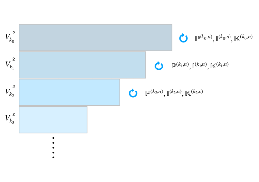
Inspired by this, we consider here a generalization of these types of models where we take the $R$-matrix to be a linear combination of the identity, permutation and trace operators, see (2.1)-(2.3), that are restricted to subspaces $V_{k_{d-1}}\subset\ldots\subset V_{k_{1}}\subset V_{k_{0}}$ see Figure 1. We recall that, in linear algebra, a flag refers to such an increasing sequence of subspaces of a vector space, and hence we name these solutions flag integrable models.

By using the boost operator method, we find three non-trivial infinite families of integrable spin chains that have such a flag structure. We refer to these as models I, II and III. These models are characterized by a set $\vec{k}$ of $d$ decreasing positive integers

$$\vec{k}=\{k_{0},k_{1},\,\ldots,\,k_{d-1}\}\,, n=k_{0}>k_{1}>\ldots>k_{d-1}\geq 1\,,$$ (1.2)

where $n$ is the dimension of the Hilbert space at each site. A subset of model II can be related to a subset of the model in [15]. Despite the simplicity of their Hamiltonians and $R$-matrices, these models have nontrivial spectra, symmetries and degeneracies. We find a fourth model, model IV, whose spectrum is purely combinatorial. For given values of $n$ and $d$, the number of possible models are ${n-1\choose d-1}$ for model I and II, and ${n-3\choose d-2}$ for models III and IV, respectively, as we will see below.

We will show that our models exhibit a type of generalized graded Lie algebra symmetry, which we will denote by $\mathfrak{gl}(k_{0}-k_{1}|\ldots|k_{d-2}-k_{d-1}|k_{d-1})$. When the flag has only two stripes i.e. $d=2$, then we return to the usual Lie superalgebra $\mathfrak{gl}(n-k|k)$. We furthermore show that Model I admits a Yangian extension of this algebra and is uniquely fixed by it.

We will also work out the nested algebraic Bethe ansatz for models I, II and III. Surprisingly, many of the transfer-matrix eigenvalues are described by infinite, singular and/or continuous Bethe roots.

2 Derivation of the models

In this section we derive the form of the flag models. Motivated by our work on Hubbard-type models and the Maassarani-Matthieu models, we will consider Hamiltonians built out of restrictions of the identity, permutation and trace operators.

2.1 The Hamiltonians

We begin by studying the direct generalization of Models 4 and 6 from [11]. We will see that these models have $R$-matrices that are rational and of difference form, and are similar to XXX-type models.

Notation

Let us first define the restricted operators that we will use to construct our integrable models. We denote

$$\mathbb{P}^{(m,n)}=\sum_{i,j=1}^{m}e_{i,j}\otimes e_{j,i}\,,$$ (2.1)

$$\mathbb{I}^{(m,n)}=\sum_{i,j=1}^{m}e_{i,i}\otimes e_{j,j}\,,$$ (2.2)

$$\mathbb{K}^{(m,n)}=\sum_{i,j=1}^{m}e_{i,j}\otimes e_{i,j}\,,$$ (2.3)

where $e_{i,j}$ is an $n\times n$ matrix such that $(e_{i,j})_{\alpha,\beta}=\delta_{i,\alpha}\delta_{j,\beta}$, and $1\leq m\leq n$. For $m=n$, the operator $\mathbb{P}^{(m,n)}$ becomes the usual permutation operator for a Hilbert space of dimension $n$, and similarly, $\mathbb{I}^{(m,n)}$ reduces to the identity matrix.

Hamiltonian

Inspired by the simple form of Models 4 and 6 from [11], we consider a similar nested structure where we combine general Hamiltonians that are built out of the building blocks of $SO(n)$ spin chains. Consider a set $\vec{k}$ of decreasing positive integers

$$\vec{k}=\{k_{0},k_{1},\,\ldots,\,k_{d-1}\}\,, n=k_{0}>k_{1}>\ldots>k_{d-1}\geq 1\,,$$ (2.4)

where $n=k_{0}$ is the dimension of the Hilbert space at each site. We take our Hamiltonian to be of the form

$$\mathcal{H}^{\vec{k}}=\sum_{i=0}^{d-1}\left(a_{i}\,\mathbb{I}^{(k_{i},n)}+b_{i}\,\mathbb{P}^{(k_{i},n)}+c_{i}\,\mathbb{K}^{(k_{i},n)}\right)\,.$$ (2.5)

At this point we do not assume the $R$-matrix is of difference form and hence the coefficients $a_{i},b_{i},c_{i}$ can depend on the inhomogeneities $\theta$ of the spin chain. We will suppress the explicit $\theta$-dependence in our notation. Nevertheless, when solving the integrability conditions, we shall see that these coefficients are in fact constants and the corresponding $R$-matrix is of difference form.

Boost operator formalism

We now proceed to insert the Ansatz (2.5) in the general boost operator formalism of [13] and classify all possible integrable Hamiltonians of this form. In order for this system to be integrable, a criterion is derived in [13] that gives a set of first-order differential equations for the coefficients of the Hamiltonian.

Recursion relations

We can obtain recursion relations for the coefficients in the Hamiltonian by acting on subspaces of our total vector space $V_{k_{0}}$. For instance, if we take a tensor product of vectors from the complement of $V_{k_{1}}$, then the only operators that act non-trivially on it will be the operators $\mathbb{P}^{(0,n)},\mathbb{I}^{(0,n)},\mathbb{K}^{(0,n)}$. In this paper, we are looking for solutions that are compatible with the general flag structures. There exist special solutions when $\vec{k}$ takes specific values; while these solutions are potentially interesting, we do not consider them in this paper.

When imposing the integrability condition on the complement of $V_{k_{1}}$, we see that only the terms with $a_{0},b_{0},c_{0}$ will contribute to the integrability condition and, consequently, they have to give an integrable Hamiltonian by themselves. We find the following equations

$$b_{0}\dot{c}_{0}=c_{0}\dot{b}_{0}\,, b_{0}c_{0}\left(b_{0}+\frac{k_{0}-2}{2}c_{0}\right)=0\,,$$ (2.6)

where the dot denotes differentiation with respect to $\theta$. There are three possible solutions to these integrability conditions, all of which are constant, namely

$$b_{0}=0, c_{0}=0, b_{0}=-\frac{k_{0}-2}{2}c_{0}.$$ (2.7)

We easily recognize the usual $SU(n)$ when $c_{0}=0$, and the $SO(n)$ spin chain when $b_{0}=\frac{2-k_{0}}{2}c_{0}$. The last case $b_{0}=0$ is a generalization of a spin chain with $SO(n)$ symmetry that was found for the case $n=4$ in [11] (see formula (4.4) in that reference).

Next we take vectors from the complement of $V_{k_{2}}$ and then $\mathbb{P}^{(1,n)},\mathbb{I}^{(1,n)},\mathbb{K}^{(1,n)}$ will contribute as well. We find equations that relate the coefficients $a_{0},b_{0},c_{0}$ and $a_{1},b_{1},c_{1}$. We generate the corresponding set of equations in Mathematica. There are on the order of 50 (dependent) equations.

Nevertheless, it can be quickly seen that the case where $c_{0}\neq 0$ implies that $a_{1}=b_{1}=c_{1}=0$. By induction this implies that there is only the contribution to our Hamiltonian from the leading part, and we keep the spin chains that we identified in the first step. We find that we need to take $c_{0}=0$ to get a new and interesting solution. When $c_{0}=0$, we can normalize our Hamiltonian such that we find two possible cases $b_{0}=0,1$. Note that $a_{0}$ can be arbitrary, since it multiplies the identity operator, and a shift of the Hamiltonian that is proportional to the identity operator is harmless.

Let us first consider the case $b_{0}=1$. The equations for $a_{1},b_{1},c_{1}$ coupled to $a_{0},b_{0},c_{0}$ can then be solved to give three different non-trivial solutions

• $a_{1}=1,~{}b_{1}=-1,~{}c_{1}=0$

• $a_{1}=-1,~{}b_{1}=-1,~{}c_{1}=0$

• $a_{1}=0,~{}b_{1}=-2,~{}c_{1}=0$

At the next level, we consider vectors from the complement of $V_{k_{2}}$ and we see that the first two solutions impose that $a_{i},b_{i},c_{i}$ all vanish for $i>1$. Hence, for these solutions our recursion terminates. The third solution, however, offers a continuation at the next level and again gives rise to three cases

• $a_{2}=1,~{}b_{2}=1,~{}c_{2}=0$

• $a_{2}=-1,~{}b_{2}=1,~{}c_{2}=0$

• $a_{2}=0,~{}b_{2}=2,~{}c_{2}=0$

Also in this instance, the first two solutions terminate the recursion again. Repeating this process, we see that we are left with two types of models. First, there is the model with the third-type solution repeated to the end:

$$H^{\textup{I},\vec{k}}=a_{0}\,\mathbb{I}^{(n,n)}+b_{0}\,\Big{[}\mathbb{P}^{(n,n)}+2\sum_{j=1}^{d-1}(-1)^{j}\mathbb{P}^{(k_{j},n)}\Big{]}\,.$$ (2.8)

It is natural to introduce $m\in[1,n]$, and to define $\bar{m}$ by

$$\bar{m}=\left\{\begin{array}[]{cc}1&k_{1}<m\leq k_{0}\\ 2&k_{2}<m\leq k_{1}\\ \vdots&\vdots\\ d&0<m<k_{d-1}\end{array}\right.\,.$$ (2.13)

The barred index indicates in which subspace our vector takes values. We can then rewrite

$$H^{\textup{I},\vec{k}}=a_{0}\,\mathbb{I}^{(n,n)}+b_{0}\ \mathcal{P}^{\vec{k}},$$ (2.14)

where

$$\mathcal{P}^{\vec{k}}(e_{i}\otimes e_{j})=(-1)^{\min(\bar{i},\bar{j})}e_{j}\otimes e_{i}.$$ (2.15)

is a generalization of the usual graded permutation operator. For a flag with two stripes this is just proportional to the usual graded permutation operator. To the best of our knowledge, this simple rational model has not been found in the literature before.

Second is the case where in the last step one of the other solutions is used

$$H^{\textup{II}_{\pm},\vec{k}}=a_{0}\,\mathbb{I}^{(n,n)}+b_{0}\,\Bigg{[}\mathbb{P}^{(n,n)}+2\Big{(}\sum_{j=1}^{d-2}(-1)^{j}\mathbb{P}^{(k_{j},n)}\Big{)}-(-1)^{d}\mathbb{P}^{(k_{d-1},n)}\pm\mathbb{I}^{(k_{d-1},n)}\Bigg{]}\,.$$ (2.16)

Third, there is a special case when $k_{d-1}=2$. In this case, we find that $\mathbb{K}^{(2)}$ can appear. Hence, we arrive at a third model given by

$$H^{\textup{III}_{\pm},\vec{k}}=a_{0}\,\mathbb{I}^{(n,n)}+b_{0}\Bigg{[}\mathbb{P}^{(n,n)}+2\Big{(}\sum_{j=1}^{d-2}(-1)^{j}\mathbb{P}^{(k_{j},n)}\Big{)}-(-1)^{d}\mathbb{P}^{(2,n)}\pm\mathbb{K}^{(2,n)}\mp\mathbb{I}^{(2,n)}\Bigg{]}\,.$$ (2.17)

Notice that the only possible $SO(N)$ type integrable Hamiltonian that is compatible with the imposed flag structure is the usual $SO(N)$ spin chain. The only other instance in which the trace operator appears is in the case $k_{d-1}=2$ as in Model III.

Let us finally consider the case with $b_{0}=c_{0}=0$. Since we can set $a_{0}=0$ without loss of generality, we find at the next step that $b_{1}=c_{1}=0$, and that $a_{1}$ is constant. By induction, this structure goes through to the other levels as well, and generically one arrives at a diagonal Hamiltonian, which is trivially integrable. However, also here there is a special case when $k_{d-1}=2$. When this is the case, we find a non-trivial Hamiltonian. This is our fourth model, which we denote by

$$H^{\textup{IV},\vec{k}}=b_{d-1}\,(\mathbb{P}^{(2,n)}-\mathbb{K}^{(2,n)})+\sum_{j=0}^{d-1}a_{j}\mathbb{I}^{(k_{j},n)}\,.$$ (2.18)

This model, however, is different from the previous ones since its spectrum is purely combinatorial: all the eigenvalues are simply integer multiples of the coefficients $a_{i}$ and $b_{d-1}$. Hence we will not consider this model much further.

2.2 $R$-matrices

In order to prove that these models are integrable, we compute the $R$-matrices that generate the Hamiltonians. We emphasize that we restrict throughout this paper to non-graded R-matrices, which satisfy the non-graded (ordinary) Yang-Baxter equation. Unsurprisingly, the $R$-matrices can be expressed in terms of the same operators as the Hamiltonians, and are easily found from the Sutherland equation [10, 11, 12, 13]

$$\left[R_{13}R_{23},H_{12}(u)\right]=\dot{R}_{13}R_{23}-R_{13}\dot{R}_{23}\,,$$ (2.19)

where the dot indicates the derivative with respect to the first spectral parameter $\dot{R}(u,v)=\partial_{u}R(u,v)$. The Sutherland equations can be derived from the Yang-Baxter equation and give a set of non-linear first-order differential equations for the $R$-matrix in terms of the Hamiltonian. Given that the $R$-matrix needs to satisfy the boundary conditions $R(u,u)=P$ and $\dot{R}(u,u)=PH$, we find that a given Hamiltonian leads to a unique $R$-matrix which is a solution of the Yang-Baxter equation.

2.2.1 Model I

The $R$-matrix corresponding to the Hamiltonian (2.8) is given by

$$R^{\textup{I},\vec{k}}(u)=(u+1)\left(\eta\,\mathbb{P}^{(n,n)}+u\,\mathbb{I}^{(n,n)}+2\,u\,\sum_{j=1}^{d-1}(-1)^{j}\mathbb{I}^{(k_{j},n)}\right)\,,$$ (2.20)

where we hereby set

$$a_{0}=\eta\,,\qquad b_{0}=1\,,$$ (2.21)

where $\eta$ has the interpretation of a quantum parameter (Planck’s constant) rather than an anisotropy parameter. We can do this since we are free to choose a normalization of the $R$-matrix and also redefine our spectral parameter. The form of this $R$-matrix is evidently very simple.

We can now decompose the $R$-matrix into the sum of the permutation matrix and a simple diagonal matrix, namely

$$R^{\textup{I},\vec{k}}(u)=(u+1)\Big{[}\eta\,\mathbb{P}^{(n,n)}+2\,u\,\mathcal{I}^{\vec{k}}\Big{]},$$ (2.22)

where $\mathcal{I}^{\vec{k}}$ is a diagonal matrix with the following $\pm 1$ entries

$$\mathcal{I}^{\vec{k}}(e_{i}\otimes e_{j})=(-1)^{\min(\bar{i},\bar{j})}e_{i}\otimes e_{j}.$$ (2.23)

To the best of our knowledge this is a new $R$-matrix.

2.2.2 Model II

The $R$-matrix corresponding to the Hamiltonian (2.16) is

$$R^{\textup{II}\pm,\vec{k}}(u)=(u+1)\left(u\mathbb{I}^{(n,n)}+\eta\,\mathbb{P}^{(n,n)}+2u\sum_{j=1}^{d-2}(-1)^{j}\mathbb{I}^{(k_{j},n)}-u(-1)^{d}\,\mathbb{I}^{(k_{d-1},n)}\pm u\mathbb{P}^{(k_{d-1},n)}\right)\,.$$ (2.24)

The first three terms coincide with the $R$-matrix for Model I, but with vector $\{k_{0},\ldots,k_{d-2}\}$. Hence, we can write it as

$$R^{\textup{II}\pm,\vec{k}}(u)=R^{\textup{I},\vec{k}-1}(u)-u(u+1)\Big{[}(-1)^{d}\,\mathbb{I}^{(k_{d-1,n)}}\pm\mathbb{P}^{(k_{d-1},n)}\Big{]}\,,$$ (2.25)

where by $R^{\textup{I},\vec{k}-1}(u)$ we denote the $R$-matrix of Model I corresponding to $\vec{k}$ with the last element dropped.

At this point, let us spell out more clearly that this R-matrix actually describes a family of models indexed by $\vec{k}$ and the $\pm$ sign. For fixed values of $n$ and $d$, there are ${n-1\choose d-1}$ possible sets of $\vec{k}$’s. For $n=k_{0}=5$, for example, we have:

• $d=1:$ only one model, corresponds to XXX;

• $d=2:$ $\{k_{1}\}$ can be equal to $k_{1}=\{\{1\},\{2\},\{3\},\{4\}\}$, so there are four sets of $\vec{k}$’s;

• $d=3:$ $\{k_{1},k_{2}\}$ can be equal to $\{k_{1},k_{2}\}=\{\{2,1\},\{3,1\},\{4,1\},\{3,2\},\{4,2\},\{4,3\}\}$, resulting in six different sets of $\vec{k}$’s;

• $d=4:$ $\{k_{1},k_{2},k_{3}\}$ can be equal to $\{\{3,2,1\},\{4,2,1\},\{4,3,1\},\{4,3,2\}\}$, which corresponds to four sets of $\vec{k}$’s;

• $d=5:$ $\{k_{1},k_{2},k_{3},k_{4}\}$ can be only equal to $\{4,3,2,1\}$.

We note that a subset of Model II can be related to the models found in [15]. Setting in the latter all $x_{\alpha,\alpha^{\prime}}=1$ and $\gamma=0$, we find the following dictionary

Model $\textup{II}^{+}$ with $d=2$	Maassarani’s model [15]
$n$	$n$
$\vec{k}=\{k_{0},k_{1}\}=\{n,n-m+1\}$	$\vec{n}=\{n_{1},n_{2},\ldots,n_{m}\}=\{1,1,\ldots,1,n-m+1\}$

The mapping between the R-matrices is as follows: removing from the $R$-matrix (2.24) the overall factor $(1+u)$, setting $d=2$ and $\eta=i$, we have

$$R^{\textup{II}+,\{k_{0},k_{1}\}}(u)=u(\mathbb{I}^{(n,n)}-\,\mathbb{I}^{(k_{1},n)})+i\,\mathbb{P}^{(n,n)}+u\mathbb{P}^{(k_{1})}\,.$$ (2.26)

Then

$$R^{\{1,1,\ldots,1,k_{1}\}}_{\rm Maassarani}(u)=(V\otimes V)R^{\textup{II}+,\{k_{0},k_{1}\}}(u)(V\otimes V)\,,$$ (2.27)

where $V$ is the $n\times n$ anti-diagonal unit matrix

$$V=\begin{pmatrix}0&0&\ldots&0&1\\ 0&0&\ldots&1&0\\ \vdots&\vdots&&\vdots&\vdots\\ 0&1&\ldots&0&0\\ 1&0&\ldots&0&0\end{pmatrix}=\sum_{i=1}^{n}e_{i,n-i+1}\,.$$ (2.28)

Inspired by the presentation of [15], we find that we can rewrite our $R$-matrix (2.24) as

$$R^{\textup{II}\pm,\vec{k}}(u)=(u+1)\left(\eta\mathbb{P}^{(n,n)}+\,u\,\mathbb{F}^{(\pm,\vec{k})}\right)\,,$$ (2.29)

where $\mathbb{F}^{(\pm,\vec{k})}$ is defined by

$$\mathbb{F}^{(\pm,\vec{k})}=\mathbb{I}^{(n,n)}-(-1)^{d}\,\mathbb{I}^{(k_{d-1},n)}\pm\mathbb{P}^{(k_{d-1},n)}+2\sum_{j=1}^{d-2}(-1)^{j}\mathbb{I}^{(k_{j},n)}\,,$$ (2.30)

which satisfies

$$\mathbb{F}^{(\pm,\vec{k})}\,\mathbb{F}^{(\pm,\vec{k})} =\mathbb{I}^{(n,n)}\,,$$ (2.31)

$$\mathbb{F}_{12}^{(\pm,\vec{k})}\mathbb{F}_{13}^{(\pm,\vec{k})}\mathbb{F}_{23}^{(\pm,\vec{k})} =\mathbb{F}_{23}^{(\pm,\vec{k})}\mathbb{F}_{13}^{(\pm,\vec{k})}\mathbb{F}_{12}^{(\pm,\vec{k})}\,.$$ (2.32)

Moreover, $\check{\mathbb{F}}^{(\pm,\vec{k})}:=\mathbb{P}^{(n,n)}\,\mathbb{F}^{(\pm,\vec{k})}$ satisfies

$$\check{\mathbb{F}}^{(\pm,\vec{k})}_{12}\check{\mathbb{F}}^{(\pm,\vec{k})}_{23}\check{\mathbb{F}}^{(\pm,\vec{k})}_{12}=\check{\mathbb{F}}^{(\pm,\vec{k})}_{23}\check{\mathbb{F}}^{(\pm,\vec{k})}_{12}\check{\mathbb{F}}^{(\pm,\vec{k})}_{23}\,.\\$$ (2.33)

In other words, $\mathbb{F}$ is a constant solution of the Yang-Baxter equation, and we can view the total $R$-matrix of Model II as a Baxterization of $\mathbb{F}$ with the constant solution. The proof for (2.31) for any $n$, $d$ and $k_{i}$ for both Models II⁺ and II^- is straightforward.

2.2.3 Model III

Model III is very similar to Model II, and only differs in a new two-dimensional term. The R-matrix for Model III (2.17) is given by

$$R^{\textup{III}\pm,\vec{k}}(u) =(u+1)\Bigg{(}u\,\mathbb{I}^{(n,n)}+\eta\,\mathbb{P}^{(n,n)}+2\,u\,\sum_{j=1}^{d-2}(-1)^{j}\,\mathbb{I}^{(k_{j},n)}$$

$$\hskip 28.45274pt+(-1)^{d+1}\,u\,\mathbb{I}^{(2,n)}\pm u\,\mathbb{K}^{(2,n)}\mp u\,\mathbb{P}^{(2,n)}\Bigg{)}\,,$$ (2.34)

where $k_{d-1}=2$.

2.2.4 Properties of R-matrices for models I, II and III

The $R$-matrices for models I, II, III satisfy some additional relations. First, we note that they all are symmetric

$$R^{t}=R\,.$$ (2.35)

Second, they are also trivially parity invariant

$$R_{21}=R_{12}\,.$$ (2.36)

Third, the $R$-matrices satisfy braiding unitarity

$$R_{12}(u)\,R_{21}(-u)\sim 1\,.$$ (2.37)

We found also some more general relations

$$R(u)\,\mathbb{P}^{(m,n)}\,R(-u)\,\mathbb{P}^{(m,n)}\sim\mathbb{I}^{(m,n)}\,,$$ (2.38)

for $m\in[1,n]$ for models I and II, and for $m\neq n-1$ for model III. For $m=n$, this corresponds to braiding unitarity (2.37). Additionally, these $R$-matrices satisfy

$$R(u)\,\mathbb{I}^{(m,n)}\,R(-u)\,\mathbb{I}^{(m,n)}\sim\mathbb{I}^{(m,n)}\,,$$ (2.39)

where again $m\in[1,n]$ for models I and II, and $m\neq n-1$ for model III.

In general, the $R$-matrices do not satisfy crossing symmetry, except for a few specific values of $k_{i}$.

2.2.5 Model IV

The R-matrix for Model IV (2.18) is given by

$$R^{\textup{IV},\vec{k}}(u)= (\eta\,u+1)\left[\mathbb{P}^{(n,n)}-\left(\prod_{j=1}^{d-2}e^{a_{j}\,u}\right)\left(1-e^{a_{d-1}\,u}\,\cosh u\right)\mathbb{P}^{(2,n)}+\right.$$

$$\left.+\left(\prod_{j=1}^{d-1}e^{a_{j}\,u}\right)\sinh u\left(\mathbb{K}^{(2,n)}-\mathbb{I}^{(2,n)}\right)-\sum_{j=1}^{d-2}\left(1-e^{a_{j}\,u}\right)\left(\prod_{i=1}^{j-1}e^{a_{i}\,u}\right)\mathbb{P}^{(k_{j},n)}\right]\,.$$ (2.40)

We see that, despite the simple form of the Hamiltonian (2.18), the corresponding R-matrix is more involved and is in fact of trigonometric type.

3 Generalized graded algebra

Usually, understanding the symmetries of the underlying models helps with explaining the degeneracies of the spectrum and further properties of the model. Given the closeness of the models to usual XXX-type models, we expect some sort of Yangian symmetry to be present. In this section we will demonstrate that models I, II and III exhibit a new type symmetry. We can fully fix model I by symmetry considerations, but for models II and III a symmetry derivation seems to be out of reach. The new symmetry is particularly interesting because it seems to describe a generalized type of Fermi statistics. For this reason we call them generalized graded algebras.

3.1 Definition

Let us first look at Model I, since this will be the model with the most symmetry. Let us define the stripes of the flag as the complements $V_{k_{i}}\backslash V_{k_{i+1}}$. Then we see that Model I obviously has $\mathfrak{gl}(k_{0}-k_{1})\oplus\ldots\oplus\mathfrak{gl}(k_{d-2}-k_{d-1})\oplus\mathfrak{gl}(k_{d-1})$ symmetry. In particular, on each stripe of the flag, we can transform the basis vectors into each other by the appropriate $\mathfrak{gl}$ transformation. For example the first stripe $V_{k_{0}}\backslash V_{k_{1}}$ is a $k_{0}-k_{1}$ dimensional subspace and has the corresponding factor of $\mathfrak{gl}(k_{0}-k_{1})$ in the symmetry algebra.

However, the symmetry generators that map between the different stripes of the flag take on a different form. This can be seen by considering the large $u$ limit on $R^{\textup{I}}$ (2.22), where it becomes diagonal but not proportional to the identity operator. This is reminiscent of the appearance of a braiding charge from the AdS/CFT correspondence [20]. So, let us try to emulate the discussion in that paper and consider the RTT representation of a Yangian algebra from the $R$-matrix (2.22).

In [20] the braiding charge appears at the lowest order in the expansion of the RTT algebra. If we do a similar expansion here, however, we find that in contradistinction to a braiding charge, the corresponding element here is not central. Hence, we are led to the introduction of a set of elements $\Gamma_{\bar{k}\bar{l}}$ that generalize the notion of a braiding charge but can have non-trivial commutation relations. Now, expanding our $R$-matrix further at large $u$, we find the next order to be the standard matrix unities $E_{ij}$.

Combining these observations, we introduce a new type of Hopf algebra $\mathcal{A}_{\gamma}$ which is a general braided version of $\mathfrak{gl}(n)$ and depends on some constants $\gamma=\pm 1$. This new algebra will contain the symmetry for model I, graded models as well as braided coproducts.

Algebra

Let us now define this new algebra. Consider generators $\Gamma_{\bar{k}\bar{l}}$ and $E_{ij}$ that satisfy the following (anti-)commutation relations

$$E_{ij}E_{kl}-\gamma_{ijkl}E_{kl}E_{ij}=\delta_{jk}E_{il}-\gamma_{ijkl}\delta_{il}E_{kj}\,,$$ (3.1)

$$E_{ij}\Gamma_{\bar{k}\bar{l}}-\gamma_{ijkl}\Gamma_{\bar{k}\bar{l}}E_{ij}=0\,,$$ (3.2)

$$[\Gamma_{\bar{a}\bar{b}},\Gamma_{\bar{c}\bar{d}}]=0\,.$$ (3.3)

Notice that from (3.1) it follows that $\gamma_{ij,kl}=\gamma_{kl,ij}$.

Coalgebra

We then introduce the following coproduct structure

$$\Delta\Gamma_{\bar{a}\bar{b}} =\Gamma_{\bar{a}\bar{b}}\otimes\Gamma_{\bar{a}\bar{b}}\,,$$ (3.4)

$$\Delta E_{ij} =E_{ij}\otimes 1+\Gamma_{\bar{i}\bar{j}}\otimes E_{ij}\,.$$ (3.5)

This coproduct is easily seen to be coassociative but it only constitutes an algebra homomorphism for certain cases. It is straightforward to check that the coproduct is compatible with (3.2) and (3.3). However, let us now apply the coproduct to (3.1). We find

$$\Delta(E_{ij}E_{kl}-\gamma_{ijkl}E_{kl}E_{ij}) =\,(E_{ij}E_{kl}-\gamma_{ijkl}E_{kl}E_{ij})\otimes 1+\Gamma_{\bar{i}\bar{j}}\Gamma_{\bar{k}\bar{l}}\otimes(E_{ij}E_{kl}-\gamma_{ijkl}E_{kl}E_{ij})$$

$$\quad+\big{[}E_{ij}\Gamma_{\bar{k}\bar{l}}-\gamma_{ijkl}\Gamma_{\bar{k}\bar{l}}E_{ij}\big{]}\otimes E_{kl}+\big{[}\Gamma_{\bar{i}\bar{j}}E_{kl}-\gamma_{ijkl}E_{kl}\Gamma_{\bar{i}\bar{j}}\big{]}\otimes E_{ij},$$

$$=(\delta_{jk}E_{il}-\gamma_{ijkl}\delta_{il}E_{kj})\otimes 1+\Gamma_{\bar{i}\bar{j}}\Gamma_{\bar{k}\bar{l}}\otimes(\delta_{jk}E_{il}-\gamma_{ijkl}\delta_{il}E_{kj}),$$

$$=\delta_{jk}\Big{[}E_{il}\otimes 1+\Gamma_{\bar{i}\bar{j}}\Gamma_{\bar{k}\bar{l}}\otimes E_{il}\Big{]}-\gamma_{ijkl}\delta_{il}\Big{[}E_{kj}\otimes 1+\Gamma_{\bar{i}\bar{j}}\Gamma_{\bar{k}\bar{l}}\otimes E_{kj}\Big{]}\,,$$ (3.6)

where we used that the second line vanishes because of (3.2). On the other hand,

$$\Delta(\delta_{jk}E_{il}-\gamma_{ijkl}\delta_{il}E_{kj}) =\delta_{jk}(E_{il}\otimes 1+\Gamma_{\bar{i}\bar{l}}\otimes E_{il})-\gamma_{ijkl}\delta_{il}(E_{kj}\otimes 1+\Gamma_{\bar{k}\bar{j}}\otimes E_{kj})\,.$$ (3.7)

Hence we see that the coproduct defines an algebra homomorphism if and only if

$$\delta_{kj}\Gamma_{\bar{i}\bar{j}}\Gamma_{\bar{k}\bar{l}}=\delta_{kj}\Gamma_{\bar{i}\bar{l}}\,.$$ (3.8)

This puts additional relations on our braiding functions $\Gamma$ that need to be satisfied for this to define a bialgebra.

Antipode

The antipode $\Sigma$ would satisfy

$$\Sigma(\Gamma_{\bar{i}\bar{j}})\Gamma_{\bar{i}\bar{j}}=1\,, \Sigma(E_{ij})\Gamma_{\bar{i}\bar{j}}=-E_{ij}\,.$$ (3.9)

This means that for any coefficients $i,j$ there should be some $i^{\prime},j^{\prime}$ such that $\Gamma_{\bar{i}\bar{j}}\Gamma_{\bar{i}^{\prime}\bar{j}^{\prime}}=1$. This imposes some further constraints on our generators in order to give a Hopf algebra.

3.2 Examples

Let us now give some examples of explicit realizations of our algebra.

Standard Lie algebra

Setting $\Gamma=1=\gamma_{ijkl}$ simply gives us the usual $\mathfrak{gl}(n)$ Lie algebra.

Grading

Let us consider a flag with two stripes and let us choose $\Gamma$ to be such that it does not commute with all algebra elements, but is idempotent $\Gamma^{2}=1$. Consider a representation of the algebra elements $E_{ij}$ and introduce a matrix $J$ that acts on the same space. We then define

$$\Gamma_{\bar{a}\bar{b}}=\left\{\begin{array}[]{cc}\bar{a}<\bar{b}&J\\ \bar{a}=\bar{b}&1\\ \bar{a}>\bar{b}&J\end{array}\right.\,,$$ (3.13)

where the matrix $J$ satisfies $J^{2}=1$. Then the antipode maps $\Gamma$ to itself and (3.8) is satisfied as well. Let us now have a look on how to interpret this model. For conciseness, let us restrict to two dimensions $(n=2)$. The coproduct takes the form

$$\Delta E_{11}=E_{11}\otimes 1+1\otimes E_{11}\,, \Delta E_{22}=E_{22}\otimes 1+1\otimes E_{22}\,,$$ (3.14)

$$\Delta E_{12}=E_{12}\otimes 1+J\otimes E_{12}\,, \Delta E_{21}=E_{21}\otimes 1+J\otimes E_{21}\,.$$ (3.15)

This exactly yields the well-known way to implement the graded tensor product using the standard tensor product by interpreting $J$ as the graded identity matrix. So, let us set

$$\gamma_{1212}=\gamma_{1221}=\gamma_{2112}=\gamma_{2121}=-1,$$ (3.16)

and the other $\gamma$’s equal to 1. Then we precisely recover $\mathfrak{gl}(1|1)$ where the coproduct is realized by using the grading matrix $J=\mathrm{diag}(1,-1)$, and we see that all the Hopf algebra relations are indeed satisfied. This straightforwardly generalizes to $\mathfrak{gl}(m|n)$.

AdS/CFT type braiding

We can make $\Gamma$ central and set $\gamma_{ijkl}=1$. This automatically satisfies all the algebra relations (3.1)-(3.3). However, the additional constraints (3.8) and (3.9) put restrictions on our choice of a braiding factor. Inspired by the braiding in AdS/CFT, let us consider the flag with two stripes, so $n=k_{0}>k_{1}$. Hence the indices on $\Gamma$ only take the values $1,2$. Now, let us define

$$\Gamma_{\bar{a}\bar{b}}=\left\{\begin{array}[]{cc}\bar{a}<\bar{b}&e^{ip}\\ \bar{a}=\bar{b}&1\\ \bar{a}>\bar{b}&e^{-ip}\end{array}\right.\,.$$ (3.20)

Then it is easy to check that (3.8) and (3.9) are satisfied assuming that the antipode maps $p\mapsto-p$, i.e. we find that $\Sigma(\Gamma_{ij})=\Gamma_{ji}$. We see that the algebra is undeformed, but that the coproduct is deformed by a central element usually referred to as a braiding factor. This algebra is simply $\mathfrak{gl}(n)$ with a braided coproduct similar to the one found in the AdS/CFT correspondence [21].

Flag models

Our flag models I, II and III satisfy a generalization of the graded algebra given above. The braiding elements $\Gamma$ are again not commutative and idempotent $\Gamma^{2}=1$. However, they take different values between different stripes of the flag. We will work out this algebra in detail in Section 3.3 and discuss its properties.

3.3 Algebra for flag model I

Let us focus here on flag model I, whose $R$-matrix has an extended symmetry that we denote by $\mathfrak{gl}(k_{0}-k_{1}|\ldots|k_{d-2}-k_{d-1}|k_{d-1})$, which we will interpret as a generalized graded algebra.

We find that for Model I, we need to make the choice that if $\bar{i}=\bar{j}$, then $\Gamma_{\bar{i}\bar{j}}=1$. If $\bar{i}\neq\bar{j}$, then $\Gamma_{\bar{i}\bar{j}}$ is given by

$$\Gamma_{\bar{i}\bar{j}}=\Gamma_{\bar{j}\bar{i}}=\prod_{l={\rm min}(\bar{i},\bar{j})}^{{\rm max}(\bar{i},\bar{j})-1}\Gamma_{k_{l}}\,,$$ (3.21)

where $\sigma_{l}$ is the $n\times n$ diagonal matrix defined by

$$\sigma_{l}=\mathop{\rm diag}\nolimits(-1,\ldots,-1_{l},1,\ldots,1_{n})\,.$$ (3.22)

Hence we see that just like for the graded algebra, $\Gamma$ takes the form of a diagonal matrix with $\pm 1$.

It is easy to check that the $R$-matrix for model I (2.20) has $\mathfrak{gl}(k_{0}-k_{1}|\ldots|k_{d-2}-k_{d-1}|k_{d-1})$ symmetry

$$\Delta^{op}E_{ij}\,R(u)=R(u)\,\Delta E_{ij}\,,\qquad i,j\in[1,n]\,,$$ (3.23)

where $\Delta E_{ij}$ is given by (3.5) and $\Delta^{op}E_{ij}$ is similarly given by

$$\Delta^{op}E_{ij}=E_{ij}\otimes\Gamma_{\bar{i}\bar{j}}+1\otimes E_{ij}\,.$$ (3.24)

We can determine the constants $\gamma_{ijkl}$ from the $\Gamma$ matrices: multiplying (3.2) on the right by $E_{ji}$, we obtain

$$E_{ij}\Gamma_{\bar{k}\bar{l}}E_{ji}=\gamma_{ijkl}\Gamma_{\bar{k}\bar{l}}E_{ii}\,,$$ (3.25)

where there is no summation over repeated indices. Since the $\Gamma$ matrices are diagonal, we see that

$$\left(\Gamma_{\bar{k}\bar{l}}\right)_{jj}E_{ii}=\gamma_{ijkl}\left(\Gamma_{\bar{k}\bar{l}}\right)_{ii}E_{ii}\,,$$ (3.26)

which implies

$$\gamma_{ijkl}=\left(\Gamma_{\bar{k}\bar{l}}\right)_{jj}/\left(\Gamma_{\bar{k}\bar{l}}\right)_{ii}\,.$$ (3.27)

Hence we also find that in this case $\gamma=\pm 1$, meaning that we are dealing with a mixture of commutation relations and anti-commutation relations.

The easiest way to see that this model is not just a usual graded algebra in disguise is the fact that $\Gamma$ appearing in the coproducts will be different depending on the operator. For usual superalgebras, all even and odd generators share the same braiding factor. As an example, let us work out the case $\vec{k}=\{3,2,1\}$. This is the first non-trivial example since it corresponds to a flag with 3 stripes. The diagonal operators $E_{ii}$ have the standard coproduct

$$\Delta E_{ii}=E_{ii}\otimes 1+1\otimes E_{ii}.$$ (3.28)

Then there are three other possibilities $E_{12},E_{13},E_{23}$, which are the operators that relate basis vectors belonging to the different stripes in the flag. This corresponds to the algebra $\mathfrak{gl}(1|1|1)$. The elements $E_{21},E_{31},E_{32}$ are simply related by transposition, which also shows that $\Gamma_{ij}=\Gamma_{ji}$.

The easiest way to represent this algebra is by taking $E_{ij}$ to be the standard matrix unities; from (3.8) it is then easy to see that $\Gamma_{12}\Gamma_{13}=\Gamma_{23}$, and we find

$$\Gamma_{12}=\begin{pmatrix}-1&0&0\\ 0&1&0\\ 0&0&1\\ \end{pmatrix}, \Gamma_{13}=\begin{pmatrix}1&0&0\\ 0&-1&0\\ 0&0&1\\ \end{pmatrix}.$$ (3.29)

From this we can compute $\gamma$ from (3.27), and we can nicely package $\gamma$ in a table

$$\begin{array}[]{c|ccccccccc}\gamma&E_{11}&E_{21}&E_{31}&E_{12}&E_{22}&E_{32}&E_{13}&E_{23}&E_{33}\\ \hline\cr E_{11}&1&1&1&1&1&1&1&1&1\\ E_{21}&1&-1&-1&-1&1&1&-1&1&1\\ E_{31}&1&-1&1&-1&1&-1&1&-1&1\\ E_{12}&1&-1&-1&-1&1&1&-1&1&1\\ E_{22}&1&1&1&1&1&1&1&1&1\\ E_{32}&1&1&-1&1&1&-1&-1&-1&1\\ E_{13}&1&-1&1&-1&1&-1&1&-1&1\\ E_{23}&1&1&-1&1&1&-1&-1&-1&1\\ E_{33}&1&1&1&1&1&1&1&1&1\\ \end{array}$$ (3.40)

Let us now have a look at the commutation relations. We see that $E_{12}$ and $E_{23}$ satisfy anti-commutations relation with itself since $\gamma_{1212}=\gamma_{2323}=-1$. Hence, these behave as odd generators. However, between each other they satisfy a usual commutation relation since $\gamma_{1223}=1$. On the other hand, $E_{13}$ and $E_{31}$ seem to be even generators ($\gamma_{1331}=1$), but satisfy anti-commutation relations with $E_{12}$ and $E_{23}$.

We conclude that we are left with a generalized graded algebra which is characterized by the number of stripes in the flag. Given the fact that model I is unique, we see that this is the unique extension of a graded-type algebra that includes multiple types of generators. A generator will satisfy either commutation or anti-commutation relations depending on which stripes it relates.

3.4 Generalized graded Yangians

There is a natural way to extend our algebra to a generalized graded Yangian. Consider the level-1 Yangian generators $\hat{E}_{ij}$ such that the following commutation relations hold

$$E_{ij}\hat{E}_{kl}-\gamma_{ijkl}\hat{E}_{kl}E_{ij}=\delta_{jk}\hat{E}_{il}-\gamma_{ijkl}\delta_{il}\hat{E}_{kj},$$ (3.41)

$$\hat{E}_{ij}{E}_{kl}-\gamma_{ijkl}{E}_{kl}\hat{E}_{ij}=\delta_{jk}\hat{E}_{il}-\gamma_{ijkl}\delta_{il}\hat{E}_{kj},$$ (3.42)

$$\hat{E}_{ij}\Gamma_{\bar{k}\bar{l}}-\gamma_{ijkl}\Gamma_{\bar{k}\bar{l}}\hat{E}_{ij}=0,$$ (3.43)

$$\Gamma_{\bar{i}\bar{j}}\hat{E}_{kl}-\gamma_{ijkl}\hat{E}_{kl}\Gamma_{\bar{i}\bar{j}}=0,.$$ (3.44)

We then introduce the standard Yangian-type coproduct

$$\Delta\hat{E}_{ij}=\hat{E}_{ij}\otimes 1+\Gamma_{\bar{i}\bar{j}}\otimes\hat{E}_{ij}-\frac{\eta}{2}\sum_{k}\Big{[}E_{kj}\otimes\Gamma_{\bar{k}\bar{j}}E_{ik}-\gamma_{ikjk}E_{ik}\otimes\Gamma_{\bar{i}\bar{k}}E_{kj}\Big{]}.$$ (3.45)

For this to define a proper Hopf algebra, we must in principle impose additional restrictions on $\Gamma,\gamma$. However, we can check that for our generalized graded algebra $\mathfrak{gl}(k_{0}-k_{1}|\ldots|k_{d-2}-k_{d-1}|k_{d-1})$ for Model I everything is compatible. Hence, if we consider the evaluation representation $\hat{E}=uE$ and the corresponding coproduct

$$\Delta\hat{E}_{ij}=u_{1}E_{ij}\otimes 1+\Gamma_{\bar{i}\bar{j}}\otimes u_{2}E_{ij}-\frac{\eta}{2}\sum_{k}\Big{[}E_{kj}\otimes\Gamma_{\bar{k}\bar{j}}E_{ik}-\gamma_{ikjk}E_{ik}\otimes\Gamma_{\bar{i}\bar{k}}E_{kj}\Big{]},$$ (3.46)

we find that it is a symmetry of the $R$-matrix of Model I. In fact, we find that the $R$-matrix of Model I is completely fixed by its generalized Yangian symmetry.

3.5 Symmetries for model II

Let us discuss the symmetries of the $R$-matrix for model II. As is clear from the form of the Hamiltonian and $R$-matrix, there is a large overlap with model I. Because of this, there is also a large overlap in symmetries. Let $e_{i}$ be the basis vectors of $V$, then the $R$-matrices of models II and I have the same action on $e_{i}\otimes e_{j}$ where ${i,j}>k_{1}$. Hence, we find that the model exhibits a $\mathfrak{gl}(k_{1}-k_{2}|\ldots|k_{d-2}-k_{d-1}|k_{d-1})$ symmetry as well as the manifest $\mathfrak{gl}(k_{0}-k_{1})$ that acts on the first indices. Moreover, also the Yangian generators $\Delta\hat{E}_{ij}$ are a symmetry for ${i,j}>k_{1}$. However, this is clearly not enough to fully fix the $R$-matrix.

Model II exhibits some additional discrete symmetries. First, models I and II are both invariant under parity. Second we have that

$$[R^{\textup{II}-},E_{\bar{1}\bar{2}}\otimes E_{\bar{1}\bar{2}}]=0, [R^{\textup{II}+},E_{\bar{1}\bar{3}}\otimes E_{\bar{1}\bar{3}}]=0.$$ (3.47)

Unfortunately, this is still not enough symmetry to fix the $R$-matrix. We have not been able to identify a remaining (discrete) symmetry that fully fixes the model.

4 Bethe ansatz for model II

We now analyze model II using nested algebraic Bethe ansatz (see e.g. [15, 16, 19, 22, 23, 24, 25, 26, 27, 28] and references therein), restricting to $k_{d-1}>1$.

4.1 First level of nesting

If we try to perform the nested Bethe ansatz procedure for model II with the R-matrix as written in Eq. (2.24), we obtain exchange relations that are not useful. A very simple local basis transformation solves this problem. We therefore use instead

$$\tilde{R}^{\textup{II}\pm,\vec{k}}(u)=\left(V\otimes V\right)R^{\textup{II}\pm,\vec{k}}(u)\left(V^{-1}\otimes V^{-1}\right)\,,$$ (4.1)

where the $n\times n$ matrix $V$ is defined in (2.28). This is exactly the same model as before because local basis transformations do not change the spectrum.

We can write the monodromy matrix for a chain of length $L$ as

$$T_{0}(u;\{\theta_{j}\}) =\tilde{R}^{\textup{II}\pm,\vec{k}}_{01}(u-\theta_{1})\,\tilde{R}^{\textup{II}\pm,\vec{k}}_{02}(u-\theta_{2})\,\ldots\,\tilde{R}^{\textup{II}\pm,\vec{k}}_{0L}(u-\theta_{L})$$ (4.2)

$$=\begin{pmatrix}\mathcal{T}_{0,0}(u;\{\theta_{j}\})&\mathcal{B}_{1}(u;\{\theta_{j}\})&\mathcal{B}_{2}(u;\{\theta_{j}\})&\cdots&\mathcal{B}_{n-1}(u;\{\theta_{j}\})\\ \mathcal{C}_{1}(u;\{\theta_{j}\})&\mathcal{T}_{1,1}(u;\{\theta_{j}\})&\mathcal{T}_{1,2}(u;\{\theta_{j}\})&\cdots&\mathcal{T}_{1,n-1}(u;\{\theta_{j}\})\\ \mathcal{C}_{2}(u;\{\theta_{j}\})&\mathcal{T}_{2,1}(u;\{\theta_{j}\})&\mathcal{T}_{2,2}(u;\{\theta_{j}\})&\cdots&\mathcal{T}_{2,n-1}(u;\{\theta_{j}\})\\ \vdots&\vdots&\vdots&\ddots&\vdots\\ \mathcal{C}_{n-1}(u;\{\theta_{j}\})&\mathcal{T}_{n-1,1}(u;\{\theta_{j}\})&\mathcal{T}_{n-1,2}(u;\{\theta_{j}\})&\cdots&\mathcal{T}_{n-1,n-1}(u;\{\theta_{j}\})\end{pmatrix}\,,$$ (4.3)

where $\{\theta_{j}\}$ are the inhomogeneities, and we suppress the superscripts $\textup{II}\pm,\vec{k}$ on the monodromy matrix to lighten the notation. The transfer matrix is therefore given by

$$t(u;\{\theta_{j}\})=\mathop{\rm tr}\nolimits_{0}T_{0}(u;\{\theta_{j}\})=\mathcal{T}_{0,0}(u;\{\theta_{j}\})+\sum_{\alpha=1}^{n-1}\mathcal{T}_{\alpha,\alpha}(u;\{\theta_{j}\}).$$ (4.4)

For a reference state such as

$$|0\rangle=\begin{pmatrix}1\\ 0\\ \vdots\\ 0\\ \end{pmatrix}^{\otimes L}\,,$$ (4.5)

we can see that

$$\mathcal{C}_{\alpha}(u;\{\theta_{j}\})|0\rangle=0\quad\forall\,\alpha=1,\ldots,n-1\,,$$ (4.6)

$$\mathcal{T}_{00}(u;\{\theta_{j}\})|0\rangle=\prod_{j=1}^{L}\left(\eta+u-\theta_{j}\right)\left(1+u-\theta_{j}\right)|0\rangle\,,$$ (4.7)

$$\mathcal{T}_{\alpha\beta}(u;\{\theta_{j}\})|0\rangle=\delta_{\alpha\beta}\,\prod_{j=1}^{L}(u-\theta_{j})(1+u-\theta_{j})|0\rangle\quad\forall\,\alpha\,,\beta=1,\ldots,n-1\,.$$ (4.8)

The operators $\mathcal{B}_{\alpha}(u;\{\theta_{j}\})$ act as creation operators. So, we can use them to define excited states

$$|\psi\rangle=\sum_{\{a_{1},\ldots,a_{m}\}}\prod_{i=1}^{m}\mathcal{B}_{a_{i}}(u_{i};\{\theta_{j}\})F^{a_{1},\cdots,a_{m}}|0\rangle$$ (4.9)

where $\{a_{i}\}$ can assume values from $1$ to $n-1$, and $\{u_{i}\}$ are the Bethe roots. By continuing the Bethe ansatz procedure we will obtain the conditions that the Bethe roots must satisfy in order for $|\psi\rangle$ to be an eigenvector of the transfer matrix $t(u;\{\theta_{j}\})$.

We have seen that the transfer matrix is given by Eq. (4.4), and we know how $\mathcal{T}_{i,j}(u,\{\theta_{j}\})$ acts on the reference state. When acting with $t(u;\{\theta_{j}\})$ on $|\psi\rangle$, we need a way to pass through all the $\mathcal{B}_{a_{i}}(u_{1};\{\theta_{j}\})$ operators. The exchange relations which allow us to do that are obtained from the RTT relation

$$\tilde{R}_{ab}^{\textup{II}\pm,\vec{k}}(u-v)\,T_{a}(u;\{\theta_{j}\})\,T_{b}(v;\{\theta_{j}\})=T_{b}(v;\{\theta_{j}\})\,T_{a}(u;\{\theta_{j}\})\,\tilde{R}_{ab}^{\textup{II}\pm,\vec{k}}(u-v)\,.$$ (4.10)

By substituting $\tilde{R}_{ab}^{\textup{II}\pm,\vec{k}}(u)$ from (4.1) and $T(u;\{\theta_{j}\})$ as in (4.3), we obtain several exchange relations. The useful ones are

$$\mathcal{T}_{0,0}(v;\{\theta_{j}\})\,\mathcal{B}_{\alpha}(u;\{\theta_{j}\}) =\frac{\eta+u-v}{u-v}\mathcal{B}_{\alpha}(u;\{\theta_{j}\})\,\mathcal{T}_{0,0}(v;\{\theta_{j}\})$$

$$\hskip 8.5359pt-\frac{\eta}{u-v}\mathcal{B}_{\alpha}(v;\{\theta_{j}\})\,\mathcal{T}_{0,0}(u;\{\theta_{j}\})\,,$$ (4.11)

where $\alpha=1,\ldots,n-1$; and

$$\mathcal{T}_{\alpha,\beta}(v;\{\theta_{j}\})\,\mathcal{B}_{\gamma}(u;\{\theta_{j}\}) =\sum_{\tau,\eta}f(u-v)\mathbb{R}_{\beta,\gamma}^{\tau,\eta}(u-v)\mathcal{B}_{\eta}(u;\{\theta_{j}\})\,\mathcal{T}_{\alpha,\tau}(v;\{\theta_{j}\})$$

$$\hskip 8.5359pt+g(u-v)\mathcal{B}_{\beta}(v;\{\theta_{j}\})\,\mathcal{T}_{\alpha,\gamma}(u;\{\theta_{j}\})\,,$$ (4.12)

where $f(u)$, $g(u)$ and $\mathbb{R}_{\beta,\gamma}^{\tau,\eta}(u)$ depend on the model, see (4.26)-(4.31) below.

Let us see how $\mathcal{T}_{0,0}(u;\{\theta_{j}\})$ acts on $|\psi\rangle$:

$$\mathcal{T}_{0,0}(u;\{\theta_{j}\})|\psi\rangle =\sum_{\{a\}}\mathcal{T}_{0,0}(u;\{\theta_{j}\})\prod_{i=1}^{m_{1}}\mathcal{B}_{a_{i}}(u_{i};\{\theta_{j}\})F^{a_{1},\cdots,a_{m_{1}}}|0\rangle$$ (4.13)

$$=\sum_{\{a\}}\mathcal{T}_{0,0}(u;\{\theta_{j}\})\mathcal{B}_{a_{1}}(u_{1};\{\theta_{j}\})\prod_{i=2}^{m_{1}}\mathcal{B}_{a_{i}}(u_{i};\{\theta_{j}\})F^{a_{1},\cdots,a_{m_{1}}}|0\rangle,$$ (4.14)

$$=\sum_{\{a\}}\frac{\eta+u_{1}-u}{u_{1}-u}\mathcal{B}_{a_{1}}(u_{1};\{\theta_{j}\})\mathcal{T}_{0,0}(u;\{\theta_{j}\})\prod_{i=2}^{m_{1}}\mathcal{B}_{a_{i}}(u_{i};\{\theta_{j}\})F^{a_{1},\cdots,a_{m_{1}}}|0\rangle$$

$$\hskip 14.22636pt-\frac{\eta}{u_{1}-u}\sum_{\{a\}}\mathcal{B}_{a_{1}}(u;\{\theta_{j}\})\mathcal{T}_{0,0}(u_{1};\{\theta_{j}\})\prod_{i=2}^{m_{1}}\mathcal{B}_{a_{i}}(u_{i};\{\theta_{j}\})F^{a_{1},\cdots,a_{m_{1}}}|0\rangle$$ (4.15)

$$=\prod_{j=1}^{L}\left(\eta+u-\theta_{j}\right)\left(1+u-\theta_{j}\right)\prod_{i=1}^{m_{1}}\frac{\eta+u_{i}-u}{u_{i}-u}|\psi\rangle$$

$$\hskip 28.45274pt+\text{unwanted terms}.$$ (4.16)

In passing from (4.14) to (4.15), we use once (4.11). We see that the second term depends on $\mathcal{B}_{a_{1}}(u;\{\theta_{j}\})$, so it cannot be written in terms of $|\psi\rangle$. As we continue to use the exchange relations to pass $\mathcal{T}_{0,0}$ through all the $\mathcal{B}$’s, we will get more and more such terms, called “unwanted terms,” which we ignore for now. In passing from (4.15) to (4.16), we just continue to use the exchange relations; and when $\mathcal{T}_{0,0}$ hits $|0\rangle$, we use (4.7).

Let us now see how $\mathcal{T}_{\alpha,\alpha}((u;\{\theta_{j}\})$ acts on $|\psi\rangle$:

$$\mathcal{T}_{\alpha,\alpha} (u;\{\theta_{j}\})|\psi\rangle=\sum_{\{a\}}\mathcal{T}_{\alpha,\alpha}(u;\{\theta_{j}\})\prod_{i=1}^{m_{1}}\mathcal{B}_{a_{i}}(u_{i};\{\theta_{j}\})F^{a_{1},\cdots,a_{m_{1}}}|0\rangle\,,$$ (4.17)

$$=\sum_{\{a\}}\mathcal{T}_{\alpha,\alpha}(u;\{\theta_{j}\})\mathcal{B}_{a_{1}}(u_{1};\{\theta_{j}\})\prod_{i=2}^{m_{1}}\mathcal{B}_{a_{i}}(u_{i};\{\theta_{j}\})F^{a_{1},\cdots,a_{m_{1}}}|0\rangle\,,$$ (4.18)

$$=\sum_{\{a\}}\sum_{\tau_{1},b_{1}}f(u_{1}-u)\mathbb{R}_{\alpha,a_{1}}^{\tau_{1},b_{1}}(u_{1}-u)\mathcal{B}_{b_{1}}(u_{1};\{\theta_{j}\})\mathcal{T}_{\alpha,\tau_{1}}(u;\{\theta_{j}\})\prod_{i=2}^{m_{1}}\mathcal{B}_{a_{i}}(u_{i};\{\theta_{j}\})F^{a_{1},\cdots,a_{m_{1}}}|0\rangle$$

$$\hskip 8.5359pt+\sum_{\{a\}}g(u_{1}-u)\mathcal{B}_{b_{1}}(u;\{\theta_{j}\})\mathcal{T}_{\alpha,a_{1}}(u_{1};\{\theta_{j}\})\prod_{i=2}^{m_{1}}\mathcal{B}_{a_{i}}(u_{i};\{\theta_{j}\})F^{a_{1},\cdots,a_{m_{1}}}|0\rangle\,,$$ (4.19)

$$=f(u_{1}-u)f(u_{2}-u)\sum_{\{a\}}\sum_{\tau_{1},\tau_{2}}\sum_{b_{1},b_{2}}\mathbb{R}_{\alpha,a_{1}}^{\tau_{1},b_{1}}(u_{1}-u)\mathbb{R}_{\tau_{1},a_{2}}^{\tau_{2},b_{2}}(u_{2}-u)\mathcal{B}_{b_{1}}(u_{1};\{\theta_{j}\})\mathcal{B}_{b_{2}}(u_{2};\{\theta_{j}\})$$

$$\hskip 22.76228pt\times\mathcal{T}_{\alpha,\tau_{2}}(u;\{\theta_{j}\})\prod_{i=3}^{m_{1}}\mathcal{B}_{a_{i}}(u_{i};\{\theta_{j}\})F^{a_{1},\cdots,a_{m_{1}}}|0\rangle+\text{unwanted terms}\,,$$ (4.20)

$$=\prod_{i=1}^{m_{1}}f(u_{i}-u)\sum_{\{b\}}\prod_{l=1}^{m_{1}}\mathcal{B}_{b_{l}}(u_{l};\{\theta_{j}\})\sum_{\{a\},\{\tau\}}\mathbb{R}_{\alpha,a_{1}}^{\tau_{1},b_{1}}(u_{1}-u)\mathbb{R}_{\tau_{1},a_{2}}^{\tau_{2},b_{2}}(u_{2}-u)\cdots\mathbb{R}_{\tau_{m_{1}-1},a_{m_{1}}}^{\tau_{m_{1}},b_{m_{1}}}(u_{m_{1}}-u)$$

$$\hskip 22.76228pt\times F^{a_{1},\cdots,a_{m_{1}}}\mathcal{T}_{\alpha,\tau_{m_{1}}}(u;\{\theta_{j}\})|0\rangle+\text{unwanted terms}\,,$$ (4.21)

$$=\prod_{i=1}^{m_{1}}f(u_{i}-u)\sum_{\{b\}}\prod_{l=1}^{m_{1}}\mathcal{B}_{b_{l}}(u_{l};\{\theta_{j}\})\sum_{\{a\},\{\tau\}}\mathbb{R}_{\alpha,a_{1}}^{\tau_{1},b_{1}}(u_{1}-u)\mathbb{R}_{\tau_{1},a_{2}}^{\tau_{2},b_{2}}(u_{2}-u)\cdots\mathbb{R}_{\tau_{m_{1}-1},a_{m_{1}}}^{\alpha,b_{m_{1}}}(u_{m_{1}}-u)$$

$$\hskip 22.76228pt\times F^{a_{1},\cdots,a_{m_{1}}}\prod_{j=1}^{L}(u-\theta_{j})(1+u-\theta_{j})|0\rangle+\text{unwanted terms}\,.$$ (4.22)

We conclude that the action of the transfer matrix (4.4) on $|\psi\rangle$ (4.9) is given by

$$t(u,\{\theta_{j}\})|\psi\rangle=\mathcal{T}_{00}(u,\{\theta_{j}\})|\psi\rangle+\sum_{\alpha=1}^{n-1}\mathcal{T}_{\alpha\alpha}(u,\{\theta_{j}\})|\psi\rangle$$

$$=\prod_{j=1}^{L}\left(\eta+u-\theta_{j}\right)\left(1+u-\theta_{j}\right)\prod_{i=1}^{m_{1}}\frac{\eta+u_{i}-u}{u_{i}-u}|\psi\rangle$$

$$+\sum_{\alpha=1}^{n-1}\left[\prod_{i=1}^{m_{1}}f(u_{i}-u)\sum_{\{b\}}\prod_{l=1}^{m_{1}}\mathcal{B}_{b_{l}}(u_{l};\{\theta_{j}\})\sum_{\{a\},\{\tau\}}\mathbb{R}_{\alpha,a_{1}}^{\tau_{1},b_{1}}(u_{1}-u)\mathbb{R}_{\tau_{1},a_{2}}^{\tau_{2},b_{2}}(u_{2}-u)\cdots\mathbb{R}_{\tau_{m_{1}-1},a_{m_{1}}}^{\alpha,b_{m_{1}}}(u_{m_{1}}-u)\right.$$

$$\left.\quad\times\,F^{a_{1}\,\cdots\,a_{m_{1}}}\prod_{j=1}^{L}(u-\theta_{j})(1+u-\theta_{j})\right]|0\rangle+\text{unwanted terms}\,.$$ (4.23)

If $|\psi\rangle$ is an eigenvector of $t(u,\{\theta_{j}\})$ so that the unwanted terms vanish, then the corresponding eigenvalue is given by

$$\Lambda(u,\{\theta_{j}\}) =\prod_{j=1}^{L}\left(\eta+u-\theta_{j}\right)\left(1+u-\theta_{j}\right)\prod_{i=1}^{m_{1}}\frac{\eta+u_{i}-u}{u_{i}-u}$$

$$+\begin{cases}(n-1)\prod_{j=1}^{L}(u-\theta_{j})(1+u-\theta_{j})&m_{1}=0\\ \Lambda_{\text{aux}}(u)\prod_{j=1}^{L}(u-\theta_{j})(1+u-\theta_{j})\prod_{i=1}^{m_{1}}f(u_{i}-u)&m_{1}\geq 1\end{cases}\,,$$ (4.24)

where $\Lambda_{\text{aux}}(u)$ is an eigenvalue of the auxiliary transfer matrix defined by

$$t_{\text{aux}}(u) =\sum_{\alpha=1}^{n-1}\sum_{\{\tau\}}\mathbb{R}_{\alpha,a_{1}}^{\tau_{1},b_{1}}(u_{1}-u)\mathbb{R}_{\tau_{1},a_{2}}^{\tau_{2},b_{2}}(u_{2}-u)\cdots\mathbb{R}_{\tau_{m_{1}-1},a_{m_{1}}}^{\alpha,b_{m_{1}}}(u_{m_{1}}-u)$$

$$=\Big{[}\mathop{\rm tr}\nolimits_{0}\mathbb{R}_{01}(u_{1}-u)\,\mathbb{R}_{02}(u_{2}-u)\,\ldots\mathbb{R}_{0m_{1}}(u_{m_{1}}-u)\Big{]}^{b_{1}b_{2}\ldots b_{m_{1}}}_{a_{1}a_{2}\ldots a_{m_{1}}}\,.$$ (4.25)

Starting with model $\textup{II}^{+}$ with a local Hilbert space of dimension $n$ (the R-matrix is $n^{2}\times n^{2}$), the corresponding $\mathbb{R}(u)$ in (4.25) is $(n-1)^{2}\times(n-1)^{2}$ and is given by

$$\mathbb{R}(u)=\begin{cases}\mathbb{P}^{(n-1,n-1)}&\text{for initial model with }k_{1}=k_{0}-1\text{ and }d=2\\ \frac{1}{1-u}\frac{1}{\eta-u}\tilde{R}^{(\textup{II}+,k_{0}-1,k_{1},..,k_{d-1})}(-u)&\text{for initial model with }k_{1}<k_{0}-1\text{ and }d\geq 2\\ \frac{1}{1+u}\frac{1}{\eta+u}\tilde{R}^{(\textup{II}-,k_{1},..,k_{d-1})}(u)&\text{for initial model with }k_{1}=k_{0}-1\text{ and }d>2\\ \end{cases}.$$ (4.26)

Also,

$$f(u)=\begin{cases}-\frac{\eta-u}{u}&\text{for all the cases with auxiliary problem given by }\tilde{R}^{+}(-u)\text{ or }\mathbb{P}^{(n-1,n-1)}\\ -\frac{\eta+u}{u}&\text{for all the cases with auxiliary problem given by }\tilde{R}^{-}(u)\end{cases}$$ (4.27)

while

$$g(u)=\frac{\eta}{u},$$ (4.28)

for all cases. In particular, starting with the R-matrix for model $\textup{II}^{+}$, we are led to an auxiliary problem that can be either related to $\textup{II}^{+}$ or to $\textup{II}^{-}$ depending on the values of $d$ and $\vec{k}$ according to Eq. (4.26).

Similarly, starting with model $\textup{II}^{-}$, the $\mathbb{R}(u)$ in (4.25) is given by

$$\mathbb{R}(u)=\begin{cases}\mathbb{P}^{(n-1,n-1)}&\text{for initial model with }k_{1}=k_{0}-1\text{ and }d=2\\ \frac{1}{1-u}\frac{1}{\eta-u}\tilde{R}^{(\textup{II}-,k_{0}-1,k_{1},..,k_{d-1})}(-u)&\text{for initial model with }k_{1}<k_{0}-1\text{ and }d\geq 2\\ \frac{1}{1+u}\frac{1}{\eta+u}\tilde{R}^{(\textup{II}+,k_{1},..,k_{d-1})}(u)&\text{for initial model with }k_{1}=k_{0}-1\text{ and }d>2.\\ \end{cases}.$$ (4.29)

Also,

$$f(u)=\begin{cases}-\frac{\eta-u}{u}&\text{for all the cases with auxiliary problem given by }\tilde{R}^{-}(-u)\\ -\frac{\eta+u}{u}&\text{for all the cases with auxiliary problem given by }\tilde{R}^{+}(u)\text{ or }\mathbb{P}^{(n-1,n-1)}\end{cases}$$ (4.30)

while

$$g(u)=\frac{\eta}{u},$$ (4.31)

for all cases.

4.2 Transfer-matrix eigenvalues

We now proceed to determine the transfer-matrix eigenvalues and Bethe equations of Model II. To this end, it is useful to introduce some further notations. Starting from the R-matrix $\tilde{R}^{\textup{II}\pm,\vec{k}}(u)$ (4.1), where $\vec{k}$ is the vector $\vec{k}=\{k_{0},k_{1},\ldots,k_{d-1}\}$ with dimension $|\vec{k}|:=d$, we define a sequence of R-matrices

$$\tilde{R}^{(l)}(u)\equiv\tilde{R}^{\mu_{l},\vec{k}^{(l)}}(u)\,,\qquad l=0,1,\ldots\,,$$ (4.32)

where $\tilde{R}^{(0)}(u)=\tilde{R}^{\textup{II}\pm,\vec{k}}(u)$, with $\mu_{0}=\pm 1$ for $\textup{II}\pm$, respectively; and $\vec{k}^{(0)}=\vec{k}$. Moreover, the vectors $\vec{k}^{(l)}$, as well as the parameters $\mu_{l}$, $\gamma_{l}$ and $\delta_{l}$, are defined for $l\geq 1$ recursively as follows:

$$\text{If }k_{1}^{(l-1)}<k_{0}^{(l-1)}-1\,,\quad\text{then }\vec{k}^{(l)}=\vec{k}^{(l-1)}-\vec{\epsilon}\,,\quad\mu_{l}=\mu_{l-1}\,,\quad\gamma_{l}=\delta_{l}=1\,;$$

$$\text{if }k_{1}^{(l-1)}=k_{0}^{(l-1)}-1\text{ and }|\vec{k}^{(l-1)}|>2\,,\quad\text{then }\vec{k}^{(l)}=\hat{\vec{k}}^{(l-1)}\,,\quad\mu_{l}=-\mu_{l-1}\,,\quad\gamma_{l}=\delta_{l}=-1\,;$$

$$\text{if }k_{1}^{(l-1)}=k_{0}^{(l-1)}-1\text{ and }|\vec{k}^{(l-1)}|=2\,,\quad\text{then }\mu_{l}=-\mu_{l-1}\,,\quad\gamma_{l}=-1\,,\quad\delta_{l}=\mu_{l-1}\,,$$ (4.33)

where $l=1,2,\ldots$, and $\gamma_{0}=\delta_{0}=1$. In the first line of (4.33), $\vec{\epsilon}$ is the vector $\vec{\epsilon}=\{1,0,\ldots,0\}$ that has the same dimension as $\vec{k}^{(l-1)}$, i.e. $|\vec{\epsilon}\,|=|\vec{k}^{(l-1)}|$. In the second line, the hat denotes dropping the first (left-most) component; hence, since $\vec{k}^{(l-1)}=\{k^{(l-1)}_{0}\,,k^{(l-1)}_{1}\,,\ldots\}$, then $\hat{\vec{k}}^{(l-1)}=\{k^{(l-1)}_{1}\,,\ldots\}$.

The sequence $\vec{k}^{(0)},\vec{k}^{(1)},\ldots$ terminates with

$$\vec{k}^{(l)}=\{k_{d-1}+1\,,k_{d-1}\}\qquad\mbox{where }l=k_{0}-k_{d-1}-1\,.$$ (4.34)

Indeed, it follows from (4.33) that $\vec{k}^{(k_{0}-k_{j})}=\{k_{j}\,,k_{j+1}\,,\ldots\,,k_{d-1}\}$ with $j=0,1,\ldots,d-2$. Hence, $\vec{k}^{(k_{0}-k_{d-2})}=\{k_{d-2}\,,k_{d-1}\}$, and therefore

$$\vec{k}^{(k_{0}-k_{d-1}-1)} =\vec{k}^{(k_{0}-k_{d-2}+(k_{d-2}-k_{d-1}-1))}=\{k_{d-2}-(k_{d-2}-k_{d-1}-1)\,,k_{d-1}\}$$

$$=\{k_{d-1}+1\,,k_{d-1}\}\,.$$ (4.35)

Examples of such sequences of $\vec{k}^{(l)}$ and $\mu_{l}$ are shown in Table 1.

Model II+ $(\mathbf{n=5})$
		$\mathbf{d=2}$			$\mathbf{d=3}$		$\mathbf{d=4}$
$\mathbf{l=0}$	$\{5,4\}^{+}$	$\{5,3\}^{+}$	$\{5,2\}^{+}$	$\{5,4,3\}^{+}$	$\{5,4,2\}^{+}$	$\{5,3,2\}^{+}$	$\{5,4,3,2\}^{+}$
	$\big{\downarrow}$	$\big{\downarrow}$	$\big{\downarrow}$	$\big{\downarrow}$	$\big{\downarrow}$	$\big{\downarrow}$	$\big{\downarrow}$
$\mathbf{l=1}$	$\mathbb{P}^{(4)}$	$\{4,3\}^{+}$	$\{4,2\}^{+}$	$\{4,3\}^{-}$	$\{4,2\}^{-}$	$\{4,3,2\}^{+}$	$\{4,3,2\}^{-}$
		$\big{\downarrow}$	$\big{\downarrow}$	$\big{\downarrow}$	$\big{\downarrow}$	$\big{\downarrow}$	$\big{\downarrow}$
$\mathbf{l=2}$		$\mathbb{P}^{(3)}$	$\{3,2\}^{+}$	$\mathbb{P}^{(3)}$	$\{3,2\}^{-}$	$\{3,2\}^{-}$	$\{3,2\}^{+}$
			$\big{\downarrow}$		$\big{\downarrow}$	$\big{\downarrow}$	$\big{\downarrow}$
$\mathbf{l=3}$			$\mathbb{P}^{(2)}$		$\mathbb{P}^{(2)}$	$\mathbb{P}^{(2)}$	$\mathbb{P}^{(2)}$

Table 1: $\vec{k}^{(l)}$ and $\mu_{l}$ for $l=0,1,\ldots,$ $k_{0}-k_{d-1}$ for model II with $\mu_{0}=+1$ and $n=5$.

Note that the $\gamma_{l}$’s satisfy

$$\gamma_{l}=\begin{cases}-1&\text{ if }l\in\{n-k_{1}\,,n-k_{2}\,,\ldots,n-k_{d-1}\}\\ \ \ 1&\text{ otherwise }\end{cases}\,.$$ (4.36)

Moreover, the $\delta_{l}$’s satisfy

$$\delta_{l}=\begin{cases}\gamma_{l}&\text{ if }l=0,1,\ldots\ldots,n-k_{d-1}-1\\ \mu_{l-1}&\text{ if }l=n-k_{d-1}\end{cases}\,.$$ (4.37)

We further define

$$\mathbb{R}^{(l)}(u) =\begin{cases}\frac{1}{(1-\gamma_{l}u)(\eta-\gamma_{l}u)}\tilde{R}^{(l)}(-\gamma_{l}u)&l=1,2,\ldots,k_{0}-k_{d-1}-1\\[7.22743pt] \mathbb{P}^{(k_{d-1}\,,k_{d-1})}&l=k_{0}-k_{d-1}\end{cases}\,,$$

$$f^{(l)}(u) =\frac{-\eta+\delta_{l}u}{u}\,,$$ (4.38)

see (4.26),(4.29).

Let us define the sequence of transfer matrices $t^{(l)}(u;\{u_{j}^{(l)}\})$ by

$$t^{(l)}(u;\{u_{j}^{(l)}\})=\mathop{\rm tr}\nolimits_{0}\tilde{R}^{(l)}_{01}(u-u_{1}^{(l)})\,\ldots\,\tilde{R}^{(l)}_{0m_{l}}(u-u_{m_{l}}^{(l)})\,,\qquad l=0,1,\ldots,k_{0}-k_{d-1}\,,$$ (4.39)

and let us denote the corresponding eigenvalues by $\Lambda^{(l)}(u;\{u_{j}^{(l)}\})$. Note that the original transfer matrix $t(u;\{\theta_{j}\})$ in (4.4) is equal (up to a similarity transformation, see (4.1)) to $t^{(0)}(u;\{\theta_{j}\})$. We wish to determine $\Lambda(u;\{\theta_{j}\}):=\Lambda^{(0)}(u;\{u_{j}^{(0)}\})$, where

$$m_{0}:=L\,,\qquad u_{j}^{(0)}:=\theta_{j}\,.$$ (4.40)

It follows from the result (4.24) that

$$\Lambda^{(l)}(u;\{u_{j}^{(l)}\})=\prod_{j=1}^{m_{l}}(\eta+u-u_{j}^{(l)})(1+u-u_{j}^{(l)})\prod_{i=1}^{m_{l+1}}\frac{\eta+u_{i}^{(l+1)}-u}{u_{i}^{(l+1)}-u}$$

$$+\Lambda_{\text{aux}}^{(l+1)}(u;\{u_{j}^{(l+1)}\})\prod_{j=1}^{m_{l}}(u-u_{j}^{(l)})(1+u-u_{j}^{(l)})\prod_{i=1}^{m_{l+1}}f^{(l+1)}(u_{i}^{(l+1)}-u)\,,\qquad l=0,1,\ldots\,,$$ (4.41)

where $\Lambda_{\text{aux}}^{(l)}(u;\{u_{j}^{(l)}\})$ is an eigenvalue of the auxiliary transfer matrix $t_{\text{aux}}^{(l)}(u;\{u_{j}^{(l)}\})$, which is given by

$$t_{\text{aux}}^{(l)}(u;\{u_{j}^{(l)}\}) =\mathop{\rm tr}\nolimits_{0}\mathbb{R}^{(l)}_{01}(u_{1}^{(l)}-u)\,\ldots\,\mathbb{R}^{(l)}_{0m_{l}}(u_{m_{l}}^{(l)}-u)\,,$$

$$=\left(\prod_{j=1}^{m_{l}}\frac{1}{(1-\gamma_{l}(u_{j}^{(l)}-u))(\eta-\gamma_{l}(u_{j}^{(l)}-u))}\right)\,t^{(l)}(\gamma_{l}u;\{\gamma_{l}u_{j}^{(l)}\})\,,$$ (4.42)

where we have passed to the second equality using (4.38) and (4.39). Hence,

$$\Lambda_{\text{aux}}^{(l)}(u;\{u_{j}^{(l)}\})=\left(\prod_{j=1}^{m_{l}}\frac{1}{(1-\gamma_{l}(u_{j}^{(l)}-u))(\eta-\gamma_{l}(u_{j}^{(l)}-u))}\right)\,\Lambda^{(l)}(\gamma_{l}u;\{\gamma_{l}u_{j}^{(l)}\})\,.$$ (4.43)

We see from (4.41) that

$$\Lambda^{(l)}(\gamma_{l}u;\{\gamma_{l}u_{j}^{(l)}\})=\prod_{j=1}^{m_{l}}(\eta+\gamma_{l}(u-u_{j}^{(l)}))(1+\gamma_{l}(u-u_{j}^{(l)}))\prod_{i=1}^{m_{l+1}}\frac{\eta+u_{i}^{(l+1)}-\gamma_{l}u}{u_{i}^{(l+1)}-\gamma_{l}u}$$

$$+\Lambda_{\text{aux}}^{(l+1)}(\gamma_{l}u;\{u_{j}^{(l+1)}\})\prod_{j=1}^{m_{l}}\gamma_{l}(u-u_{j}^{(l)})(1+\gamma_{l}(u-u_{j}^{(l)}))\prod_{i=1}^{m_{l+1}}f^{(l+1)}(u_{i}^{(l+1)}-\gamma_{l}u)\,.$$ (4.44)

We conclude that the eigenvalue of the auxiliary transfer matrix $t_{\text{aux}}^{(l)}(u;\{u_{j}^{(l)})$ is given by

$$\Lambda_{\text{aux}}^{(l)}(u;\{u_{j}^{(l)}\})=\prod_{i=1}^{m_{l+1}}\frac{\eta+u_{i}^{(l+1)}-\gamma_{l}u}{u_{i}^{(l+1)}-\gamma_{l}u}$$

$$+\Lambda_{\text{aux}}^{(l+1)}(\gamma_{l}u;\{u_{j}^{(l+1)}\})\prod_{j=1}^{m_{l}}\frac{\gamma_{l}(u-u_{j}^{(l)})}{\eta+\gamma_{l}(u-u_{j}^{(l)})}\prod_{i=1}^{m_{l+1}}\frac{-\eta+\delta_{l+1}(u_{i}^{(l+1)}-\gamma_{l}u)}{u_{i}^{(l+1)}-\gamma_{l}u}\,,$$

$$\qquad\qquad l=1,\ldots,k_{0}-k_{d-1}-1\,,$$ (4.45)

where we have used (4.38), (4.43) and (4.44). For $l=k_{0}-k_{d-1}$, we see from (4.38) that $\mathbb{R}^{(l)}=\mathbb{P}^{(k_{d-1}\,,k_{d-1})}$ is independent of the spectral parameter, and we find

$$\Lambda_{\text{aux}}^{(k_{0}-k_{d-1})}=\begin{cases}\exp\left(\frac{2\pi ip}{m_{k_{0}-k_{d-1}}}\right)\,,\quad p=0,1,\ldots,m_{k_{0}-k_{d-1}}-1\,,&\text{ if }m_{k_{0}-k_{d-1}}\neq 0\\ k_{d-1}&\text{ if }m_{k_{0}-k_{d-1}}=0\\ \end{cases}\,.$$ (4.46)

Let us define $\Lambda_{\text{aux}}^{(0)}(u;\{\theta_{j}\})$ by (4.45) with $l=0$, keeping in mind (4.40). That is,

$$\Lambda_{\text{aux}}^{(0)}(u;\{\theta_{j}\}) =\prod_{i=1}^{m_{1}}\frac{\eta+u_{i}^{(1)}-u}{u_{i}^{(1)}-u}$$

$$+\Lambda_{\text{aux}}^{(1)}(u;\{u_{j}^{(1)}\})\prod_{j=1}^{L}\frac{u-\theta_{j}}{\eta+u-\theta_{j}}\prod_{i=1}^{m_{1}}\frac{-\eta+\delta_{1}(u_{i}^{(1)}-u)}{u_{i}^{(1)}-u}\,.$$ (4.47)

It follows from (4.24) that

$$\Lambda(u;\{\theta_{j}\})=\prod_{j=1}^{L}(\eta+u-\theta_{j})(1+u-\theta_{j})\Lambda_{\text{aux}}^{(0)}(u;\{\theta_{j}\})\,,$$ (4.48)

where $\Lambda_{\text{aux}}^{(0)}(u;\{\theta_{j}\})$ can be determined recursively using (4.47), (4.45) and (4.46).

4.3 Bethe equations

The conditions that the expressions (4.45) for $\Lambda_{\text{aux}}^{(l)}(u;\{u_{j}^{(l)}\})$ have vanishing residues at the poles $u=\gamma_{l}u_{i}^{(l+1)}$ lead (after the shift $l\mapsto l-1$) to the following Bethe equations for $\{u_{i}^{(l)}\}$

$$\prod_{j=1}^{m_{l-1}}\frac{\eta-\gamma_{l-1}(u_{j}^{(l-1)}-\gamma_{l-1}u_{i}^{(l)})}{\gamma_{l-1}(\gamma_{l-1}u_{i}^{(l)}-u_{j}^{(l-1)})} =\Lambda^{(l)}_{\text{aux}}(u_{i}^{(l)};\{u_{j}^{(l)}\})\prod_{j\neq i;j=1}^{m_{l}}\frac{\delta_{l}(u_{j}^{(l)}-u_{i}^{(l)})-\eta}{u_{j}^{(l)}-u_{i}^{(l)}+\eta}\,,$$

$$\qquad i=1,2,\ldots,m_{l}\,,\qquad l=1,2,\ldots,k_{0}-k_{d-1}\,,$$ (4.49)

$$\Lambda^{(l)}_{\text{aux}}(u_{i}^{(l)};\{u_{j}^{(l)}\}) =\prod_{j=1}^{m_{l+1}}\frac{\eta+u_{j}^{(l+1)}-\gamma_{l}u_{i}^{(l)}}{u_{j}^{(l+1)}-\gamma_{l}u_{i}^{(l)}}\,,\quad l=1,2,\ldots,k_{0}-k_{d-1}-1\,,$$ (4.50)

and $\Lambda^{(k_{0}-k_{d-1})}_{\text{aux}}$ is given in (4.46).

In summary, the eigenvalues $\Lambda(u;\{\theta_{j}\})$ of the transfer matrix $t(u;\{\theta_{j}\})$ (4.4) are given by (4.45)-(4.48), where $\{u_{i}^{(l)}\}$ are solutions of the Bethe equations (4.49), (4.50).

Remarkably, these Bethe equations can be brought to a form similar to those of usual $\mathfrak{gl}(m|n-m)$ spin chains. Indeed, let us define the rescaled Bethe roots

$$\tilde{u}^{(l)}_{j}:=\chi_{l}\,u^{(l)}_{j}\,,\qquad\chi_{l}:=\prod_{l^{\prime}<l}\gamma_{l^{\prime}}\,,$$ (4.51)

in terms of which the Bethe equations (4.49), (4.50) can be rewritten as

$$(\delta_{l})^{m_{l}-1} =\prod_{j=1}^{m_{l-1}}\frac{\tilde{u}^{(l)}_{i}-\tilde{u}^{(l-1)}_{j}}{\tilde{u}^{(l)}_{i}-\tilde{u}^{(l-1)}_{j}+\chi_{l}\eta}\prod_{j\neq i}^{m_{l}}\frac{\tilde{u}^{(l)}_{i}-\tilde{u}^{(l)}_{j}+\delta_{l}\chi_{l}\eta}{\tilde{u}^{(l)}_{i}-\tilde{u}^{(l)}_{j}-\chi_{l}\eta}$$

$$\times\prod_{j=1}^{m_{l+1}}\frac{\tilde{u}^{(l)}_{i}-\tilde{u}^{(l+1)}_{j}-\chi_{l+1}\eta}{\tilde{u}^{(l)}_{i}-\tilde{u}^{(l+1)}_{j}}\,,\qquad i=1,\ldots,m_{l}\,,\qquad l=1,\ldots,k_{0}-k_{d-1}-1\,,$$

$$\frac{(\delta_{l})^{m_{l}-1}}{\Lambda^{(k_{0}-k_{d-1})}_{\text{aux}}} =\prod_{j=1}^{m_{l-1}}\frac{\tilde{u}^{(l)}_{i}-\tilde{u}^{(l-1)}_{j}}{\tilde{u}^{(l)}_{i}-\tilde{u}^{(l-1)}_{j}+\chi_{l}\eta}\prod_{j\neq i}^{m_{l}}\frac{\tilde{u}^{(l)}_{i}-\tilde{u}^{(l)}_{j}+\delta_{l}\chi_{l}\eta}{\tilde{u}^{(l)}_{i}-\tilde{u}^{(l)}_{j}-\chi_{l}\eta}\,,\quad i=1,\ldots,m_{l}\,,\quad l=k_{0}-k_{d-1}\,.$$ (4.52)

Finally, in terms of the shifted Bethe roots

$$\tilde{\tilde{u}}^{(l)}_{j}:=\tilde{u}^{(l)}_{j}+\frac{\eta}{2}\sum_{i=1}^{l}\chi_{i}\,,$$ (4.53)

the Bethe equations (4.52) take the more symmetric form

$$(\delta_{l})^{m_{l}-1} =\prod_{j=1}^{m_{l-1}}\frac{\tilde{\tilde{u}}^{(l)}_{i}-\tilde{\tilde{u}}^{(l-1)}_{j}-\frac{\eta}{2}\chi_{l}}{\tilde{\tilde{u}}^{(l)}_{i}-\tilde{\tilde{u}}^{(l-1)}_{j}+\frac{\eta}{2}\chi_{l}}\prod_{j\neq i}^{m_{l}}\frac{\tilde{\tilde{u}}^{(l)}_{i}-\tilde{\tilde{u}}^{(l)}_{j}+\delta_{l}\chi_{l}\eta}{\tilde{\tilde{u}}^{(l)}_{i}-\tilde{\tilde{u}}^{(l)}_{j}-\chi_{l}\eta}\prod_{j=1}^{m_{l+1}}\frac{\tilde{\tilde{u}}^{(l)}_{i}-\tilde{\tilde{u}}^{(l+1)}_{j}-\frac{\eta}{2}\chi_{l+1}}{\tilde{\tilde{u}}^{(l)}_{i}-\tilde{\tilde{u}}^{(l+1)}_{j}+\frac{\eta}{2}\chi_{l+1}}\,,$$

$$\qquad\qquad\qquad i=1,\ldots,m_{l}\,,\qquad l=1,\ldots,k_{0}-k_{d-1}-1\,,$$

$$\frac{(\delta_{l})^{m_{l}-1}}{\Lambda^{(k_{0}-k_{d-1})}_{\text{aux}}} =\prod_{j=1}^{m_{l-1}}\frac{\tilde{\tilde{u}}^{(l)}_{i}-\tilde{\tilde{u}}^{(l-1)}_{j}-\frac{\eta}{2}\chi_{l}}{\tilde{\tilde{u}}^{(l)}_{i}-\tilde{\tilde{u}}^{(l-1)}_{j}+\frac{\eta}{2}\chi_{l}}\prod_{j\neq i}^{m_{l}}\frac{\tilde{\tilde{u}}^{(l)}_{i}-\tilde{\tilde{u}}^{(l)}_{j}+\delta_{l}\chi_{l}\eta}{\tilde{\tilde{u}}^{(l)}_{i}-\tilde{\tilde{u}}^{(l)}_{j}-\chi_{l}\eta}\,,\quad i=1,\ldots,m_{l}\,,\quad l=k_{0}-k_{d-1}\,,$$ (4.54)

where $\Lambda^{(k_{0}-k_{d-1})}_{\text{aux}}$ is defined in equation (4.46).

The Bethe equations (4.54) are therefore simply given by

$$(\delta_{l})^{m_{l}-1}z^{-1}_{l}(p)=\prod_{l^{\prime}=1}^{k_{0}-k_{d-1}}\prod_{j=1}^{m_{l^{\prime}}}{}^{{}^{\prime}}\frac{\tilde{\tilde{u}}^{(l)}_{i}-\tilde{\tilde{u}}^{(l^{\prime})}_{j}+\frac{\eta}{2}c_{l,l^{\prime}}}{\tilde{\tilde{u}}^{(l)}_{i}-\tilde{\tilde{u}}^{(l^{\prime})}_{j}-\frac{\eta}{2}c_{l,l^{\prime}}}\,,\qquad i=1,\ldots,m_{l}\,,\qquad l=1,\ldots,k_{0}-k_{d-1}\,,$$ (4.55)

where the primed product omits the $j=i$ term if $l^{\prime}=l$, and $c_{l,l^{\prime}}$ is given by

diagonal: $$c_{l,l} =\begin{cases}2\chi_{l}&\text{ if }\quad\delta_{l}=+1\\ 0&\text{ if }\quad\delta_{l}=-1\end{cases}\,,$$

off-diagonal: $$c_{l,l^{\prime}} =\begin{cases}-\chi_{l}&\text{ if }\quad l^{\prime}=l-1\\ -\chi_{l^{\prime}}&\text{ if }\quad l^{\prime}=l+1\\ \ \ 0&\text{ otherwise }\end{cases}\,,$$ (4.56)

where $\chi_{l}$ (4.51) is $\pm 1$. The function $z_{l}(p)$ is given by

$$z_{l}(p)=\begin{cases}1&\text{ if }\qquad l=1,\ldots,k_{0}-k_{d-1}-1\\ \Lambda^{(k_{0}-k_{d-1})}_{\text{aux}}&\text{ if }\qquad l=k_{0}-k_{d-1}\end{cases}\,.$$ (4.57)

Note that $c_{l,l+1}=c_{l+1,l}$, and therefore $c_{l,l^{\prime}}$ is symmetric. Moreover, in view of (4.37),

$$\sum_{l^{\prime}}c_{l,l^{\prime}}=-\chi_{l}(1+\gamma_{l})+c_{l,l}=0\,,\qquad l=2,\ldots,k_{0}-k_{d-1}-1\,.$$ (4.58)

Hence, $c_{l,l^{\prime}}$ can be identified as the Cartan matrix for a (potentially non-distinguished) $\mathfrak{gl}(m|n-m)$ Kac-Dynkin diagram. For example, for the case $\{5,4,3,2\}^{+}$ (for which $\delta_{1}=\delta_{2}=-1\,,\delta_{3}=1$), the corresponding diagram is shown in Fig. 2; fermionic nodes (for which $c_{l,l}=0$) are denoted by a cross. However, compared with usual $\mathfrak{gl}(m|n-m)$ spin chains, the LHS of the Bethe equations (4.54) has additional phases; moreover, the transfer-matrix eigenvalues (4.48), which can be re-expressed in terms of the redefined Bethe roots $\tilde{\tilde{u}}^{(l)}_{i}$, are not the standard ones.

Since model II has rank $k_{0}-1$, one would expect it to have an equal number of Bethe equations; however, there are in fact only $k_{0}-k_{d-1}$ such equations (4.55). The “missing” Bethe equations are hidden in the condition (4.46). For example, the Kac-Dynkin diagram in Fig. 2 for a model of rank four has one less node than expected. Therefore, despite the similarities with $\mathfrak{gl}(m|n-m)$, this model is significantly different.

Figure 2: Dynkin diagram for the model II case $\{5,4,3,2\}^{+}$

We have checked the completeness of this Bethe ansatz solution numerically for small values of $L,d,\vec{k}$ by using (4.45)-(4.50) to solve for the eigenvalues of the homogeneous transfer matrix (all $\theta_{j}=0$), and comparing with the corresponding results obtained by exact diagonalization, see e.g. Tables 6,7,8. We observe the presence of infinite Bethe roots, as well as singular (exceptional) solutions of the Bethe equations. While we can account for all distinct eigenvalues (although not their degeneracies), there is one caveat: we find instances with repeated singular Bethe roots (such as the last line of Table 7), where the roots indeed give the eigenvalue through the TQ equation (4.48), but the Bethe equations are not all satisfied (at least naively), which we leave as a problem for future investigation. Based on these studies, we conjecture that the values of $\{m_{l}\}$ can be restricted as follows

$$m_{0}\geq m_{1}\geq m_{2}\geq\ldots\geq m_{k_{0}-k_{d-1}}\,,$$ (4.59)

where $m_{0}:=L$.

5 Bethe ansatz for model I

We now analyze model I using nested algebraic Bethe ansatz, again restricting to $k_{d-1}>1$.

5.1 First level of nesting

Similarly to model II, for model I we perform the Bethe ansatz for the gauge-transformed R-matrix

$$\tilde{R}^{\textup{I},\vec{k}}(u)=\left(V\otimes V\right)R^{\textup{I},\vec{k}}(u)\left(V^{-1}\otimes V^{-1}\right)\,,$$ (5.1)

where $V$ is defined in (2.28), and $R^{\textup{I},\vec{k}}(u)$ is given in (2.20).

This model has much in common with model II, so for the parts of the analysis that coincide, we refer to the previous section in order to avoid repeating formulas. The equations from (4.3) to (4.9) remain the same. In particular, the action of the operators $\mathcal{C}_{\alpha},\,\mathcal{T}_{00}$ and $\mathcal{T}_{\alpha\beta}$ on the reference state $|0\rangle$ do not change. The exchange relations are again given by (4.11) and (4.12), except $\mathbb{R}(u)$ is now given by

$$\mathbb{R}(u)=\begin{cases}\frac{1}{\eta+u}R^{(gl_{n-1})}(u)&\text{for initial model with }k_{1}=k_{0}-1\text{ and }d=2\\ \frac{1}{1+u}\frac{1}{\eta+u}\tilde{R}^{(\textup{I},k_{0}-1,k_{1},..,k_{d-1})}(u)&\text{for initial model with }k_{1}=k_{0}-1\text{ and }d>2\\ \frac{1}{1-u}\frac{1}{\eta-u}\tilde{R}^{(\textup{I},k_{1},..,k_{d-1})}(-u)&\text{for initial model with }k_{1}<k_{0}-1\text{ and }d\geq 2\\ \end{cases}$$ (5.2)

where $R^{gl_{m}}(u)$ is the $m^{2}\times m^{2}$ R-matrix given by

$$R^{(gl_{m})}(u)=\eta\mathbb{P}^{(m,n)}+u\mathbb{I}^{(m,n)}.$$ (5.3)

The functions $f(u)$ and $g(u)$ are defined as

$$f(u)=\begin{cases}\frac{\eta-u}{-u}&\text{for initial model with }k_{1}<k_{0}-1\text{ and }d\geq 2\\ \frac{\eta+u}{-u}&\text{for initial model with }k_{1}=k_{0}-1\text{ and }d\geq 2\\ \end{cases}$$ (5.4)

$$g(u)=\frac{\eta}{u}.$$ (5.5)

Hence, except for the explicit forms of $\mathbb{R}(u)$ and $f(u)$, Eqs. (4.17)-(4.22) remain the same. We conclude that the eigenvalues of the transfer matrix are given by

$$\Lambda(u,\{\theta_{j}\}) =\prod_{j=1}^{L}\left(\eta+u-\theta_{j}\right)\left(1+u-\theta_{j}\right)\prod_{j=1}^{m_{1}}\frac{\eta+u_{j}-u}{u_{j}-u}$$

$$+\Lambda_{\text{aux}}(u)\prod_{j=1}^{L}(u-\theta_{j})(1+u-\theta_{j})\prod_{j=1}^{m_{1}}f(u_{j}-u)\,,$$ (5.6)

where $\Lambda_{\text{aux}}(u)$ is an eigenvalue of the auxiliary transfer matrix (4.25).

5.2 Transfer-matrix eigenvalues

In the following we will recursively construct the TQ and Bethe equations for this model, in a similar way as for model II. As we will show, the main difference is that in the “last” step of the nesting procedure, for $d=2$ and $k_{1}=k_{0}-1$, we have $\mathbb{R}(u)\sim R^{gl_{k_{d-1}}}(u)$ for model I, instead of $\mathbb{R}(u)\sim\mathbb{P}^{(k_{d-1},k_{d-1})}$ for model II. Consequently, an extra recursion procedure will be needed for model I.

We define a sequence of R-matrices

$$\tilde{R}^{(l)}(u)\equiv\tilde{R}^{\vec{k}^{(l)}}(u)\,,\qquad l=0,1,\ldots\,,k_{d-1}$$ (5.7)

where $\tilde{R}^{(0)}(u)=\tilde{R}^{\vec{k}}(u)$ and $\vec{k}^{(0)}=\vec{k}$. Moreover, the vectors $\vec{k}^{(l)}$, as well as the parameter $\gamma_{l}$, similarly to section 4 are defined for $l\geq 1$ recursively as follows:

$$\text{If }k_{1}^{(l-1)}<k_{0}^{(l-1)}-1\,,\quad\text{then }\vec{k}^{(l)}=\vec{k}^{(l-1)}-\vec{\epsilon}\,,\quad\gamma_{l}=1\,;$$

$$\text{if }k_{1}^{(l-1)}=k_{0}^{(l-1)}-1\text{ and }|\vec{k}^{(l-1)}|>2\,,\quad\text{then }\vec{k}^{(l)}=\hat{\vec{k}}^{(l-1)}\,,\quad\gamma_{l}=-1\,;$$

$$\text{if }k_{1}^{(l-1)}=k_{0}^{(l-1)}-1\text{ and }|\vec{k}^{(l-1)}|=2\,,\quad\text{then }\gamma_{l}=-1\,.$$ (5.8)

As before, $\vec{\epsilon}$ is the vector $\vec{\epsilon}=\{1,0,\ldots,0\}$ that has the same dimension as $\vec{k}^{(l-1)}$, i.e. $|\vec{\epsilon}\,|=|\vec{k}^{(l-1)}|$. Furthermore, the hat denotes dropping the first (left-most) component; hence, since $\vec{k}^{(l-1)}=\{k^{(l-1)}_{0}\,,k^{(l-1)}_{1}\,,\ldots\}$, then $\hat{\vec{k}}^{(l-1)}=\{k^{(l-1)}_{1}\,,\ldots\}$. Examples of such $\vec{k}^{(l)}$ sequences are shown in Table 2.

The $\gamma_{l}$’s again satisfy (4.36), for $l=1,...,k_{0}-k_{d-1}$.

We also define

$$\mathbb{R}^{(l)}(u) =\begin{cases}\frac{1}{(1-\gamma_{l}u)(\eta-\gamma_{l}u)}\tilde{R}^{(l)}(-\gamma_{l}u)&l=1,2,\ldots,k_{0}-k_{d-1}-1\\[7.22743pt] \frac{1}{\eta+u}R^{gl_{k_{d-1}}}(u)&l=k_{0}-k_{d-1}\end{cases}\,,$$

$$f^{(l)}(u) =\frac{-\eta+\gamma_{l}u}{u}\,,$$ (5.9)

where $R^{gl_{k_{d-1}}}(u)$ is given by (5.3).

Model I $(\mathbf{n=5}$)
		$\mathbf{d=2}$			$\mathbf{d=3}$		$\mathbf{d=4}$
$\mathbf{l=0}$	$\{5,4\}$	$\{5,3\}$	$\{5,2\}$	$\{5,4,3\}$	$\{5,4,2\}$	$\{5,3,2\}$	$\{5,4,3,2\}$
	$\big{\downarrow}$	$\big{\downarrow}$	$\big{\downarrow}$	$\big{\downarrow}$	$\big{\downarrow}$	$\big{\downarrow}$	$\big{\downarrow}$
$\mathbf{l=1}$	$\text{gl}_{4}$	$\{4,3\}$	$\{4,2\}$	$\{4,3\}$	$\{4,2\}$	$\{4,3,2\}$	$\{4,3,2\}$
		$\big{\downarrow}$	$\big{\downarrow}$	$\big{\downarrow}$	$\big{\downarrow}$	$\big{\downarrow}$	$\big{\downarrow}$
$\mathbf{l=2}$		$\text{gl}_{3}$	$(3,2)$	$\text{gl}_{3}$	$\{3,2\}$	$\{3,2\}$	$\{3,2\}$
			$\big{\downarrow}$		$\big{\downarrow}$	$\big{\downarrow}$	$\big{\downarrow}$
$\mathbf{l=3}$			$\text{gl}_{2}$		$\text{gl}_{2}$	$\text{gl}_{2}$	$\text{gl}_{2}$

Table 2: $\vec{k}^{(l)}$ for $l=0,1,\ldots,k_{0}-k_{d-1}$ for model I with $n=5$.

The first part of this calculation is very similar to the one for model II, with only a few sign modifications. We again start by defining a sequence of transfer matrices $t^{(l)}(u;\{u_{j}^{(l)}\})$ as in (4.39)

$$t^{(l)}(u;\{u_{j}^{(l)}\})=\mathop{\rm tr}\nolimits_{0}\tilde{R}^{(l)}_{01}(u-u_{1}^{(l)})\,\ldots\,\tilde{R}^{(l)}_{0m_{l}}(u-u_{m_{l}}^{(l)})\,,\qquad l=0,1,\ldots,k_{0}-k_{d-1}\,,$$ (5.10)

and denoting the corresponding eigenvalues by $\Lambda^{(l)}(u;\{u_{j}^{(l)}\})$. We obtain as in (4.41)

$$\Lambda^{(l)}(u;\{u_{j}^{(l)}\})=\prod_{j=1}^{m_{l}}(\eta+u-u_{j}^{(l)})(1+u-u_{j}^{(l)})\prod_{j=1}^{m_{l+1}}\frac{\eta+u_{j}^{(l+1)}-u}{u_{j}^{(l+1)}-u}$$

$$+\Lambda_{\text{aux}}^{(l+1)}(u;\{u_{j}^{(l+1)}\})\prod_{j=1}^{m_{l}}(u-u_{j}^{(l)})(1+u-u_{j}^{(l)})\prod_{j=1}^{m_{l+1}}f^{(l+1)}(u_{j}^{(l+1)}-u)\,,$$

$$\qquad\qquad\qquad\qquad\qquad l=0,1,\ldots\,,k_{0}-k_{d-1}$$ (5.11)

Eqs. (4.42)-(4.44) do not change, and from them and (5.11) we obtain (cf. (4.45))

$$\Lambda_{\text{aux}}^{(l)}(u;\{u_{j}^{(l)}\})=\prod_{j=1}^{m_{l+1}}\frac{\eta+u_{j}^{(l+1)}-\gamma_{l}u}{u_{j}^{(l+1)}-\gamma_{l}u}$$

$$+\Lambda_{\text{aux}}^{(l+1)}(\gamma_{l}u;\{u_{j}^{(l+1)}\})\prod_{j=1}^{m_{l}}\frac{\gamma_{l}(u-u_{j}^{(l)})}{\eta+\gamma_{l}(u-u_{j}^{(l)})}\prod_{j=1}^{m_{l+1}}\frac{-\eta+\gamma_{l+1}(u_{j}^{(l+1)}-\gamma_{l}u)}{u_{j}^{(l+1)}-\gamma_{l}u}\,,$$

$$\qquad\qquad l=1,\ldots,k_{0}-k_{d-1}-1\,.$$ (5.12)

The second part of the calculation is dedicated to computing $\Lambda_{\text{aux}}^{(k_{0}-k_{d-1})}$, which appears in (5.12) for the final value $l=k_{0}-k_{d-1}-1$. We shall see that this requires the diagonalization of $gl_{m}$-type transfer matrices. We therefore first define a sequence of $gl_{m}$-type R-matrices

$$r^{(l)}(u)=R^{gl_{k_{0}-l}}(u)\,,\qquad l=k_{0}-k_{d-1},k_{0}-k_{d-1}+1,\ldots\,,k_{0}-2\,,$$ (5.13)

where $R^{gl_{m}}$ is defined in (5.3). Consider then a sequence of transfer matrices $\tau^{(l)}(u;\{u_{j}^{(l)}\})$

$$\tau^{(l)}(u;\{u_{j}^{(l)}\})=\mathop{\rm tr}\nolimits_{0}r^{(l)}_{01}(u-u_{1}^{(l)})\,\ldots\,r^{(l)}_{0m_{l}}(u-u_{m_{l}}^{(l)})\,,\qquad l=k_{0}-k_{d-1},\ldots,k_{0}-2\,.$$ (5.14)

The corresponding eigenvalue $\lambda^{(l)}(u;\{u_{j}^{(l)}\})$ is well known to be given by

$$\lambda^{(l)}(u;\{u_{j}^{(l)}\}) =\prod_{j=1}^{m_{l}}(\eta+u-u_{j}^{(l)})\prod_{j=1}^{m_{l+1}}\frac{\eta+u_{j}^{(l+1)}-u}{u_{j}^{(l+1)}-u}$$

$$+\lambda_{\text{aux}}^{(l+1)}(u;\{u_{j}^{(l+1)}\})\prod_{j=1}^{m_{l}}(u-u_{j}^{(l)})\prod_{j=1}^{m_{l+1}}\phi^{(l+1)}(u_{j}^{(l+1)}-u)\,,$$

$$\qquad\qquad\qquad l=k_{0}-k_{d-1},\ldots\,,k_{0}-2,$$ (5.15)

where $\phi^{(l)}(u)$ is given by

$$\phi^{(l)}(u)=\frac{-\eta+u}{u}\,,$$ (5.16)

and $\lambda_{\text{aux}}^{(l)}(u;\{u_{j}^{(l)}\})$ is an eigenvalue of the auxiliary transfer matrix

$$\tau_{\text{aux}}^{(l)}(u;\{u_{j}^{(l)}\})=\mathop{\rm tr}\nolimits_{0}\mathbb{R}^{(l)}_{01}(u_{1}^{(l)}-u)\,\ldots\,\mathbb{R}^{(l)}_{0m_{l}}(u_{m_{l}}^{(l)}-u)\,,$$ (5.17)

where $\mathbb{R}^{(l)}(u)$ is given by

$$\mathbb{R}^{(l)}(u)=\frac{1}{\eta-u}\,r^{(l)}(-u)\,,\qquad l=k_{0}-k_{d-1}+1,\ldots\,,k_{0}-2\,,$$ (5.18)

and $r^{(l)}(u)$ was defined in (5.13). It follows from (5.18) that $\tau_{\text{aux}}^{(l)}$ (5.17) can be related to $\tau^{(l)}$ (5.14)

$$\tau_{\text{aux}}^{(l)}(u;\{u_{j}^{(l)}\})=\left(\prod_{j=1}^{m_{l}}\frac{1}{(\eta-(u_{j}^{(l)}-u))}\right)\,\tau^{(l)}(u;\{u_{j}^{(l)}\})\,,$$ (5.19)

and similarly for the corresponding eigenvalues

$$\lambda_{\text{aux}}^{(l)}(u;\{u_{j}^{(l)}\}) =\left(\prod_{j=1}^{m_{l}}\frac{1}{(\eta-(u_{j}^{(l)}-u))}\right)\,\lambda^{(l)}(u;\{u_{j}^{(l)}\})$$ (5.20)

$$=\prod_{j=1}^{m_{l+1}}\frac{\eta+u_{j}^{(l+1)}-u}{u_{j}^{(l+1)}-u}$$

$$+\lambda_{\text{aux}}^{(l+1)}(u;\{u_{j}^{(l+1)}\})\prod_{j=1}^{m_{l}}\frac{u-u_{j}^{(l)}}{\eta+u-u_{j}^{(l)}}\prod_{j=1}^{m_{l+1}}\frac{\eta+u-u_{j}^{(l+1)}}{u-u_{j}^{(l+1)}}\,,$$

$$\qquad\qquad\qquad l=k_{0}-k_{d-1}+1,\ldots\,,k_{0}-2\,,$$ (5.21)

where we have passed to (5.21) using (5.15), and $\lambda_{\text{aux}}^{(k_{0}-1)}(u;\{u_{j}^{(k_{0}-1)}\})\equiv 1$.

We are finally ready to compute $\Lambda_{\text{aux}}^{(k_{0}-k_{d-1})}$. Recalling from (5.9) that $\mathbb{R}^{(l)}$ for $l=k_{0}-k_{d-1}$ is proportional to $R^{gl_{k_{d-1}}}$, and recalling the definitions of the transfer matrices $t_{\text{aux}}^{(l)}$ (4.42) and $\tau^{(l)}$ (5.14), we see that

$$\Lambda_{\text{aux}}^{(k_{0}-k_{d-1})}(u;\{u_{j}^{(k_{0}-k_{d-1})}\}) =\frac{\lambda^{(k_{0}-k_{d-1})}(-u;\{-u_{j}^{(k_{0}-k_{d-1})}\})}{\prod_{j=1}^{m_{k_{0}-k_{d-1}}}(\eta+u_{j}^{(k_{0}-k_{d-1})}-u)}$$

$$=\lambda_{\text{aux}}^{(k_{0}-k_{d-1})}(-u;\{-u_{j}^{(k_{0}-k_{d-1})}\})\,.$$ (5.22)

To pass to the second line, we have used (5.20) to define $\lambda_{\text{aux}}^{(l)}$ for $l=k_{0}-k_{d-1}$.

The full result for $\Lambda^{(0)}(u;\{u_{j}^{(0)}\})$ is therefore obtained by starting from $l=0$ in Eq. (5.11), and then using Eqs. (5.12), (5.22) and (5.21).

5.3 Bethe equations

For this model, the Bethe equations for $\{u_{j}^{(l)}\}$ have two sources, depending on whether $l$ is smaller or larger than $k_{0}-k_{d-1}$. The first set of Bethe equations, as in model II, comes from shifting $l\mapsto l-1$ in Eq. (5.12) and requiring the vanishing of residues at the poles $u=\gamma_{l-1}u_{i}^{(l)}$. This leads to

$$\prod_{j=1}^{m_{l-1}}\frac{\eta-\gamma_{l-1}(u_{j}^{(l-1)}-\gamma_{l-1}u_{i}^{(l)})}{\gamma_{l-1}(\gamma_{l-1}u_{i}^{(l)}-u_{j}^{(l-1)})} =\prod_{j\neq i;j=1}^{m_{l}}\frac{\gamma_{l}(u_{j}^{(l)}-u_{i}^{(l)})-\eta}{u_{j}^{(l)}-u_{i}^{(l)}+\eta}\prod_{j=1}^{m_{l+1}}\frac{\eta+u_{j}^{(l+1)}-\gamma_{l}u_{i}^{(l)}}{u_{j}^{(l+1)}-\gamma_{l}u_{i}^{(l)}}\,,$$

$$\qquad i=1,2,\ldots,m_{l}\,,\qquad l=1,2,\ldots,k_{0}-k_{d-1}\,.$$ (5.23)

Let us now turn to the second set of Bethe equations. By requiring the vanishing of the residues at the poles $u=-u_{i}^{(k_{0}-k_{d-1}+1)}$ in $\lambda_{\text{aux}}^{(k_{0}-k_{d-1})}(-u,\{-u_{j}^{(k_{0}-k_{d-1})}\})$, we obtain the Bethe equations for $l=k_{0}-k_{d-1}+1$. Similarly, by requiring vanishing residues at the poles $u=-u_{i}^{(l)}$ in $\lambda_{\text{aux}}^{(l-1)}(-u,\{u_{j}^{(l-1)}\})$, we obtain the Bethe equations for $l=k_{0}-k_{d-1}+2,\ldots,k_{0}-1$. Explicitly, the second set of Bethe equations is given by

$$1 =\lambda_{\text{aux}}^{(l)}(u_{i}^{(l)};\{u_{j}^{(l)}\})\prod_{j=1}^{m_{l-1}}\frac{u_{i}^{(l)}-\gamma_{l-1}u_{j}^{(l-1)}}{u_{i}^{(l)}-\gamma_{l-1}u_{j}^{(l-1)}+\eta}\prod_{j\neq i;j=1}^{m_{l}}\frac{u_{j}^{(l)}-u_{i}^{(l)}-\eta}{u_{j}^{(l)}-u_{i}^{(l)}+\eta}\,,$$

$$\qquad i=1,\ldots,m_{l},\,\qquad l=k_{0}-k_{d-1}+1,\ldots,k_{0}-1\,,$$ (5.24)

$$\lambda_{\text{aux}}^{(l)}(u_{i}^{(l)};\{u_{j}^{(l)}\})=\begin{cases}\prod_{j=1}^{m_{l+1}}\frac{\eta+u_{j}^{(l+1)}-u_{i}^{(l)}}{u_{j}^{(l+1)}-u_{i}^{(l)}}&l=k_{0}-k_{d-1}+1,\ldots,k_{0}-2\\ 1&l=k_{0}-1\end{cases}\,.$$ (5.25)

Notice that $\gamma_{l}$ had so far been defined only for $l=1,...,k_{0}-k_{d-1}$, with $\gamma_{k_{0}-k_{d-1}}=-1$ (4.36). In (5.24), we introduced $k_{d-1}+1$ additional $\gamma_{l}$ defined by

$$\gamma_{l}=1,\qquad l=k_{0}-k_{d-1}+1,...,k_{0}-1\,.$$ (5.26)

As we did for the Bethe equations of model II (4.55), here we can also simplify the Bethe equations (5.23)-(5.25) using the transformations (4.51) and (4.53), resulting in simply

$$(\gamma_{l})^{m_{l}-1}=\prod_{l^{\prime}=1}^{k_{0}-1}\prod_{j=1}^{m_{l^{\prime}}}{}^{{}^{\prime}}\frac{\tilde{\tilde{u}}^{(l)}_{i}-\tilde{\tilde{u}}^{(l^{\prime})}_{j}+\frac{\eta}{2}c_{l,l^{\prime}}}{\tilde{\tilde{u}}^{(l)}_{i}-\tilde{\tilde{u}}^{(l^{\prime})}_{j}-\frac{\eta}{2}c_{l,l^{\prime}}}\,,\qquad i=1,\ldots,m_{l}\,,\qquad l=1,\ldots,k_{0}-1\,,$$ (5.27)

where the primed product omits the $j=i$ term if $l^{\prime}=l$, and $c_{l,l^{\prime}}$ is given by

diagonal: $$c_{l,l} =\begin{cases}2\chi_{l}&\text{ if }\quad\gamma_{l}=+1\\ 0&\text{ if }\quad\gamma_{l}=-1\end{cases}\,,$$

off-diagonal: $$c_{l,l^{\prime}} =\begin{cases}-\chi_{l}&\text{ if }\quad l^{\prime}=l-1\\ -\chi_{l^{\prime}}&\text{ if }\quad l^{\prime}=l+1\\ \ \ 0&\text{ otherwise }\end{cases}\,,$$ (5.28)

where $\chi_{l}$ (4.51) is $\pm 1$. As an example, the Dynkin diagram for the case $\{5,4,3,2\}$ (for which $\gamma_{1}=\gamma_{2}=\gamma_{3}=-1\,,\gamma_{4}=1$), is shown in Fig. 3.

Contrary to model II, the number of Bethe equations for model I is equal to the rank. However, the Bethe equations have extra factors of $(-1)^{m_{l}-1}$ in comparison with the usual $\mathfrak{gl}(m|n-m)$ model due to the LHS of (5.27); this point is discussed further in Appendix A for the case $n=3$.

Figure 3: Dynkin diagram for the model I case $\{5,4,3,2\}$

We have checked the completeness of this Bethe ansatz solution numerically for small values of $L,d,\vec{k}$ by using (5.11), (5.12), (5.21) - (5.25) to solve for the eigenvalues, and comparing with corresponding results obtained by direct diagonalization of the transfer matrix, see Tables 9, 10, 11. As in the case of model II, we observe the existence of infinite Bethe roots, as well as singular solutions of the Bethe equations. We also find some continuous solutions (i.e., with arbitrary Bethe roots) , which here is presumably related to the presence of infinite Bethe roots. The transfer-matrix eigenvalues do not depend on the values of the arbitrary Bethe roots.

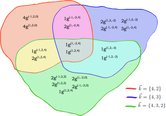
Before closing this section, we remark that there is significant overlap in the spectra of transfer matrices for different values of $d$ and $\vec{k}$. This is illustrated for model I in Fig. 4, where an eigenvalue $\Lambda(u)$ of the homogeneous transfer matrix (i.e. all $\theta_{j}=0$) with $L=2$ is denoted by $q\,\text{g}^{(\alpha_{1},\alpha_{2},\alpha_{3})}$, where

$$\Lambda(u)=\text{g}^{(\alpha_{1},\alpha_{2},\alpha_{3})}\equiv(1+u)^{2}\left(\alpha_{1}\eta^{2}+\alpha_{2}\eta u+\alpha_{3}u^{2}\right)\,,$$ (5.29)

and $q$ is its degeneracy (multiplicity).

Figure 4: Transfer-matrix eigenvalues for model I with $L=2$ and different values of $d$ and $\vec{k}$, see Eq. (5.29). Note that some $\text{g}^{(\alpha_{1},\alpha_{2},\alpha_{3})}$ (such as $\text{g}^{(1,-2,4)}$) appear more than once.

6 Bethe ansatz for model III

6.1 Transfer-matrix eigenvalues

For model III, we recall (2.34) that not only $k_{0}$ is fixed as $k_{0}=n$, but also $k_{d-1}$ is fixed as $k_{d-1}=2$. The vector $\vec{k}$ is therefore given by

$$\vec{k}=(n,k_{1},...,k_{d-2},2),\quad\text{with}\quad n=k_{0}>k_{1}>k_{2}>...>k_{d-2}>k_{d-1}=2.$$ (6.1)

There are therefore ${n-3\choose d-2}$ models of III⁺ type, and an equal number of III^- type.

The nested algebraic Bethe ansatz for model III can be performed in a similar way as for models I and II, the main difference appearing in the final step. As before, we perform the Bethe ansatz for the gauge-transformed R-matrix

$$\tilde{R}^{\textup{III}\pm,\vec{k}}(u)=\left(V\otimes V\right)R^{\textup{III}\pm,\vec{k}}(u)\left(V^{-1}\otimes V^{-1}\right)\,,$$ (6.2)

where $V$ is given in (2.28), and $R^{\textup{III}\pm,\vec{k}}(u)$ is given by (2.34). The first level of nesting is basically the same as for model I, also resulting in (5.6); what changes are the explicit forms of $\mathbb{R}$ and $f(u)$. For model III^±, the nesting procedure results in the following rule

$$\mathbb{R}(u)=\begin{cases}\frac{1}{1-u}\frac{1}{\eta-u}\tilde{R}^{(\textup{III}\pm,k_{0}-1,k_{1},...,k_{d-2},2)}(-u)&\text{if}\quad k_{1}<k_{0}-1\text{ and }k_{0}>3\\ \frac{1}{1+u}\frac{1}{\eta+u}\tilde{R}^{(\textup{III}\mp,k_{1},...,k_{d-2},2)}(u)&\text{if}\quad k_{1}=k_{0}-1\text{ and }k_{0}>3\\ \frac{1}{\eta}r(u,\delta_{0})&\text{if}\quad k_{0}=3\text{ and }k_{1}=2.\end{cases}\,,$$ (6.3)

with

$$f(u)=\begin{cases}\frac{-\eta+u}{u}&\text{if}\quad k_{1}<k_{0}-1\text{ and }k_{0}>3\\ \frac{-\eta-u}{u}&\text{if}\quad k_{1}=k_{0}-1\text{ and }k_{0}>3\\ -\frac{\eta}{u}&\text{if}\quad k_{0}=3\text{ and }k_{1}=2\end{cases}\,,$$ (6.4)

while $g(u)$ is again defined as

$$g(u)=\frac{\eta}{u}\,.$$ (6.5)

The nesting procedure ends with $\vec{k}=(3,2)$, for which (see Eq. (6.3))

$$\mathbb{R}(u)=\frac{1}{\eta}r(u,\delta_{0})\,,$$ (6.6)

where

$$r(u,\delta_{0})=\begin{pmatrix}\eta&0&0&\delta_{0}u\\ 0&0&\eta-\delta_{0}u&0\\ 0&\eta-\delta_{0}u&0&0\\ \delta_{0}u&0&0&\eta\end{pmatrix}\,,$$ (6.7)

and

$$\delta_{0}=\begin{cases}-1&\text{ if }\quad\vec{k}=\{3,2\}^{+}\\ +1&\text{ if }\quad\vec{k}=\{3,2\}^{-}\end{cases}\,.$$ (6.8)

We bring this R-matrix to the usual six-vertex form by a basis transformation

$$\tilde{r}(u,\delta_{0}) =(U\otimes U)\,r(u,\delta_{0})\,(U^{-1}\otimes U^{-1})$$ (6.9)

$$=\begin{pmatrix}\eta-\delta_{0}u&0&0&0\\ 0&\delta_{0}u&\eta&0\\ 0&\eta&\delta_{0}u&0\\ 0&0&0&\eta-\delta_{0}u\end{pmatrix}\,,$$ (6.10)

where

$$U=\begin{pmatrix}1&i\\ i&1\end{pmatrix}\,.$$ (6.11)

We henceforth use $\tilde{r}(u,\delta_{0})$ instead of $r(u,\delta_{0})$.

We again define a sequence of R-matrices

$$\tilde{R}^{(l)}(u)\equiv\tilde{R}^{\mu_{l},\vec{k}^{(l)}}(u)\,,\qquad l=0,1,\ldots\,k_{0}-2\,,$$ (6.12)

where $\mu_{l}$ and $\vec{k}^{(l)}$ are constructed via the iterative procedure

$$\text{if }k_{1}^{(l-1)}<k_{0}^{(l-1)}-1\,,\quad\text{then }\vec{k}^{(l)}=\vec{k}^{(l-1)}-\vec{\epsilon}\,,\quad\mu_{l}=\mu_{l-1}\,,\quad\gamma_{l}=+1\,;$$

$$\text{if }k_{1}^{(l-1)}=k_{0}^{(l-1)}-1\,,\quad\text{then }\vec{k}^{(l)}=\hat{\vec{k}}^{(l-1)}\,,\quad\mu_{l}=-\mu_{l-1}\,,\quad\gamma_{l}=-1\,;$$ (6.13)

where $\vec{\epsilon}$ and $\hat{\vec{k}}$ are defined as in models I and II. Examples of such sequences of $\vec{k}^{(l)}$ and $\mu_{l}$ are shown in Table 3.

Model III+ $(\mathbf{n=5})$
	$\mathbf{d=2}$		$\mathbf{d=3}$	$\mathbf{d=4}$
$\mathbf{l=0}$	$\{5,2\}^{+}$	$\{5,4,2\}^{+}$	$\{5,3,2\}^{+}$	$\{5,4,3,2\}^{+}$
	$\big{\downarrow}$	$\big{\downarrow}$	$\big{\downarrow}$	$\big{\downarrow}$
$\mathbf{l=1}$	$\{4,2\}^{+}$	$\{4,2\}^{-}$	$\{4,3,2\}^{+}$	$\{4,3,2\}^{-}$
	$\big{\downarrow}$	$\big{\downarrow}$	$\big{\downarrow}$	$\big{\downarrow}$
$\mathbf{l=2}$	$\{3,2\}^{+}$	$\{3,2\}^{-}$	$\{3,2\}^{-}$	$\{3,2\}^{+}$
	$\big{\downarrow}$	$\big{\downarrow}$	$\big{\downarrow}$	$\big{\downarrow}$
$\mathbf{l=3}$	6-vertex	6-vertex	6-vertex	6-vertex

Table 3: $\vec{k}^{(l)}$ and $\mu_{l}$ for $l=0,1,\ldots,k_{0}-2$ for model III with $\mu_{0}=+1$ and $n=5$.

The $\gamma_{l}$’s again satisfy (4.36), but only for $l=1,\ldots,k_{0}-3$. For the final two $l$-values, we define

$$\gamma_{l}=-1\,,\qquad l=k_{0}-2\,,k_{0}-1$$ (6.14)

for later convenience, see (6.27), (6.28).

Also

$$\mathbb{R}^{(l)}(u) =\begin{cases}\frac{1}{(1-\gamma_{l}u)(\eta-\gamma_{l}u)}\tilde{R}^{(l)}(-\gamma_{l}u)&l=1,2,\ldots,k_{0}-3\\[7.22743pt] \frac{1}{\eta}\tilde{r}(u,\delta_{0})&l=k_{0}-2\end{cases}\,,$$ (6.15)

$$f^{(l)}(u) =\begin{cases}\frac{-\eta+\gamma_{l}u}{u}&l=1,...,k_{0}-3\\ \frac{-\eta}{u}&l=k_{0}-2\end{cases}\,,$$ (6.16)

where $\tilde{r}(u,\delta_{0})$ was defined in (6.10).

Transfer matrices can be constructed as in (5.10)

$$t^{(l)}(u;\{u_{j}^{(l)}\})=\mathop{\rm tr}\nolimits_{0}\tilde{R}^{(l)}_{01}(u-u_{1}^{(l)})\,\ldots\,\tilde{R}^{(l)}_{0m_{l}}(u-u_{m_{l}}^{(l)})\,,\qquad l=0,1,\ldots,k_{0}-2\,,$$ (6.17)

whose eigenvalues $\Lambda^{(l)}(u;\{u_{j}^{(l)}\})$ are given, as in (5.11), by

$$\Lambda^{(l)}(u;\{u_{j}^{(l)}\})=\prod_{j=1}^{m_{l}}(\eta+u-u_{j}^{(l)})(1+u-u_{j}^{(l)})\prod_{j=1}^{m_{l+1}}\frac{\eta+u_{j}^{(l+1)}-u}{u_{j}^{(l+1)}-u}$$

$$+\Lambda_{\text{aux}}^{(l+1)}(u;\{u_{j}^{(l+1)}\})\prod_{j=1}^{m_{l}}(u-u_{j}^{(l)})(1+u-u_{j}^{(l)})\prod_{j=1}^{m_{l+1}}f^{(l+1)}(u_{j}^{(l+1)}-u)\,,$$

$$\qquad\qquad\qquad\qquad\qquad l=0,1,\ldots\,,k_{0}-2$$ (6.18)

As before, $\Lambda_{\text{aux}}^{(l)}(u;\{u_{j}^{(l)}\})$ are eigenvalues of $t_{\text{aux}}^{(l)}(u;\{u_{j}^{(l)}\})$, which is defined by

$$t_{\text{aux}}^{(l)}(u;\{u_{j}^{(l)}\}) =\mathop{\rm tr}\nolimits_{0}\mathbb{R}^{(l)}_{01}(u_{1}^{(l)}-u)\,\ldots\,\mathbb{R}^{(l)}_{0m_{l}}(u_{m_{l}}^{(l)}-u)\,,$$

$$=\begin{cases}\left(\prod_{j=1}^{m_{l}}\frac{1}{(1-\gamma_{l}(u_{j}^{(l)}-u))(\eta-\gamma_{l}(u_{j}^{(l)}-u))}\right)\,t^{(l)}(\gamma_{l}u;\{\gamma_{l}u_{j}^{(l)}\})\,,&l=1,...,k_{0}-3\\ \frac{1}{\eta^{m_{l}}}t^{(k_{0}-2)}(-u,\{-u_{j}^{(k_{0}-2)}\})&l=k_{0}-2\end{cases}\,,$$ (6.19)

where we used (6.15), and $t^{(k_{0}-2)}(u,\{u_{j}^{(k_{0}-2)}\})$ is given by

$$t^{(k_{0}-2)}(u;\{u_{j}^{(k_{0}-2)}\}) =\mathop{\rm tr}\nolimits_{0}\tilde{r}^{(k_{0}-2)}_{01}(u-u_{1}^{(k_{0}-2)},\delta_{0})\,\ldots\,\tilde{r}^{(k_{0}-2)}_{0m_{k_{0}-2}}(u-u_{m_{k_{0}-2}}^{(k_{0}-2)},\delta_{0})\,,$$ (6.20)

which has eigenvalues

$$\Lambda^{(k_{0}-2)}(u,\{u_{j}^{(k_{0}-2)}\})= \prod_{j=1}^{m_{k_{0}-2}}\left(\eta-\delta_{0}(u-u_{j}^{(k_{0}-2)})\right)\prod_{j=1}^{m_{k_{0}-1}}\frac{\eta+\delta_{0}(u-u_{j}^{(k_{0}-1)})}{-\delta_{0}(u-u_{j}^{(k_{0}-1)})}$$

$$+\prod_{j=1}^{m_{k_{0}-2}}\left(\delta_{0}(u-u_{j}^{(k_{0}-2)})\right)\prod_{j=1}^{m_{k_{0}-1}}\frac{\eta-\delta_{0}(u-u_{j}^{(k_{0}-1)})}{\delta_{0}(u-u_{j}^{(k_{0}-1)})}.$$ (6.21)

The auxiliary eigenvalues are therefore

$$\Lambda_{\text{aux}}^{(l)}(u;\{u_{j}^{(l)}\})=\begin{cases}\left(\prod_{j=1}^{m_{l}}\frac{1}{(1-\gamma_{l}(u_{j}^{(l)}-u))(\eta-\gamma_{l}(u_{j}^{(l)}-u))}\right)\,\Lambda^{(l)}(\gamma_{l}u;\{\gamma_{l}u_{j}^{(l)}\})&l=1,...,k_{0}-3\\ \frac{1}{\eta^{m_{k_{0}-2}}}\Lambda^{(k_{0}-2)}(-u;\{-u_{j}^{(k_{0}-2)}\})&l=k_{0}-2\end{cases}\,.$$ (6.22)

More explicitly, for $l=1,\ldots,k_{0}-4$, the auxiliary eigenvalues are given by

$$\Lambda_{\text{aux}}^{(l)}(u;\{u_{j}^{(l)}\})=\prod_{j=1}^{m_{l+1}}\frac{\eta+u_{j}^{(l+1)}-\gamma_{l}u}{u_{j}^{(l+1)}-\gamma_{l}u}$$

$$+\Lambda_{\text{aux}}^{(l+1)}(\gamma_{l}u;\{u_{j}^{(l+1)}\})\prod_{j=1}^{m_{l}}\frac{\gamma_{l}(u-u_{j}^{(l)})}{\eta+\gamma_{l}(u-u_{j}^{(l)})}\prod_{j=1}^{m_{l+1}}\frac{-\eta+\gamma_{l+1}(u_{j}^{(l+1)}-\gamma_{l}u)}{u_{j}^{(l+1)}-\gamma_{l}u}\,,$$

$$\qquad\qquad l=1,\ldots,k_{0}-4\,;$$ (6.23)

while for $l=k_{0}-3$ we have

$$\Lambda_{\text{aux}}^{(k_{0}-3)}(u;\{u_{j}^{(k_{0}-3)}\})=\prod_{j=1}^{m_{k_{0}-2}}\frac{\eta+u_{j}^{(k_{0}-2)}-\gamma_{k_{0}-3}u}{u_{j}^{(k_{0}-2)}-\gamma_{k_{0}-3}u}$$

$$+\Lambda_{\text{aux}}^{(k_{0}-2)}(\gamma_{k_{0}-3}u;\{u_{j}^{(k_{0}-2)}\})\prod_{j=1}^{m_{k_{0}-3}}\frac{\gamma_{k_{0}-3}(u-u_{j}^{(k_{0}-3)})}{\eta+\gamma_{k_{0}-3}(u-u_{j}^{(k_{0}-3)})}\prod_{j=1}^{m_{k_{0}-2}}\frac{-\eta}{u_{j}^{(k_{0}-2)}-\gamma_{k_{0}-3}u}\,,$$ (6.24)

and finally for $l=k_{0}-2$

$$\Lambda_{\text{aux}}^{(k_{0}-2)}(\gamma_{k_{0}-3}u;\{u_{j}^{(k_{0}-2)}\})= \prod_{j=1}^{m_{k_{0}-2}}\frac{\eta+\delta_{0}(\gamma_{k_{0}-3}u-u_{j}^{(k_{0}-2)})}{\eta}\prod_{j=1}^{m_{k_{0}-1}}\frac{\eta-\delta_{0}(\gamma_{k_{0}-3}u+u_{j}^{(k_{0}-1)})}{\delta_{0}(\gamma_{k_{0}-3}u+u_{j}^{(k_{0}-1)})}$$

$$+\prod_{j=1}^{m_{k_{0}-2}}\frac{-\delta_{0}(\gamma_{k_{0}-3}u-u_{j}^{(k_{0}-2)})}{\eta}\prod_{j=1}^{m_{k_{0}-1}}\frac{\eta+\delta_{0}(\gamma_{k_{0}-3}u+u_{j}^{(k_{0}-1)})}{-\delta_{0}(\gamma_{k_{0}-3}u+u_{j}^{(k_{0}-1)})}\,.$$ (6.25)

The equations (6.23)-(6.25) were obtained using (6.22) together with equations (6.18) and (6.21). Having obtained $\Lambda_{\text{aux}}^{(l)}(u,\{u_{j}^{(l)}\})$ for all values of $l$ (6.23)-(6.25), we can use them together with (6.18) to compute $\Lambda^{(0)}(u,\{u_{j}^{(0)}\})$.

6.2 Bethe equations

We now obtain the corresponding Bethe equations. The first set comes from requiring that $\Lambda_{\text{aux}}^{(l)}(u;\{u_{j}^{(l)}\})$ in (6.23) have vanishing residues at the poles $u=\gamma_{l}u_{i}^{(l+1)}$, and then shifting $l\mapsto l-1$

$$\prod_{j=1}^{m_{l-1}}\frac{\eta+u_{i}^{(l)}-\gamma_{l-1}u_{j}^{(l-1)}}{u_{i}^{(l)}-\gamma_{l-1}u_{j}^{(l-1)}} =\prod_{j\neq i;j=1}^{m_{l}}\frac{\gamma_{l}(u_{j}^{(l)}-u_{i}^{(l)})-\eta}{u_{j}^{(l)}-u_{i}^{(l)}+\eta}\prod_{j=1}^{m_{l+1}}\frac{\eta+u_{j}^{(l+1)}-\gamma_{l}u_{i}^{(l)}}{u_{j}^{(l+1)}-\gamma_{l}u_{i}^{(l)}}\,,$$

$$\qquad i=1,2,\ldots,m_{l}\,,\qquad l=1,2,\ldots,k_{0}-3\,.$$ (6.26)

In order to obtain the two remaining sets of Bethe equations, we first substitute (6.25) into (6.24), and then require the vanishing of the residues of $\Lambda_{\text{aux}}^{(k_{0}-3)}(u;\{u_{j}^{(k_{0}-3)}\})$ at both poles $u=\gamma_{k_{0}-3}u_{i}^{(k_{0}-2)}$ and $u=\gamma_{k_{0}-3}u_{i}^{(k_{0}-1)}$. The result is

$$\prod_{j=1}^{m_{k_{0}-3}}\frac{\eta+u_{i}^{(k_{0}-2)}-\gamma_{k_{0}-3}u_{j}^{(k_{0}-3)}}{u_{i}^{(k_{0}-2)}-\gamma_{k_{0}-3}u_{j}^{(k_{0}-3)}} =\prod_{j\neq i;j=1}^{m_{k_{0}-2}}\frac{\delta_{0}(u_{i}^{(k_{0}-2)}-u_{j}^{(k_{0}-2)})+\eta}{u_{i}^{(k_{0}-2)}-u_{j}^{(k_{0}-2)}-\eta}$$

$$\times\prod_{j=1}^{m_{k_{0}-1}}\frac{\eta+\delta_{0}(\gamma_{k_{0}-2}u_{i}^{(k_{0}-2)}-u_{j}^{(k_{0}-1)})}{-\delta_{0}(\gamma_{k_{0}-2}u_{i}^{(k_{0}-2)}-u_{j}^{(k_{0}-1)})}\,,$$

$$\hskip 85.35826pti=1,...,m_{k_{0}-2}\,,$$ (6.27)

$$1 =(-1)^{m_{k_{0}-2}}\prod_{j=1}^{m_{k_{0}-2}}\frac{u_{i}^{(k_{0}-1)}-\gamma_{k_{0}-1}u_{j}^{(k_{0}-2)}}{u_{i}^{(k_{0}-1)}-\gamma_{k_{0}-1}u_{j}^{(k_{0}-2)}-\delta_{0}\eta}\prod_{j\neq i;j=1}^{m_{k_{0}-1}}\frac{u_{i}^{(k_{0}-1)}-u_{j}^{(k_{0}-1)}-\delta_{0}\eta}{u_{i}^{(k_{0}-1)}-u_{j}^{(k_{0}-1)}+\delta_{0}\eta}\,,$$

$$\hskip 99.58464pti=1,...,m_{k_{0}-1}\,.$$ (6.28)

Following a similar procedure as for models I and II (see transformations (4.51) and (4.53)), we find that the Bethe equations (6.26)-(6.28) can be brought to the form

$$(\gamma_{l})^{m_{l}-1}z_{l}=\prod_{l^{\prime}=1}^{k_{0}-1}\prod_{j=1}^{m_{l^{\prime}}}{}^{{}^{\prime}}\frac{\tilde{\tilde{u}}^{(l)}_{i}-\tilde{\tilde{u}}^{(l^{\prime})}_{j}+\frac{\eta}{2}c_{l,l^{\prime}}}{\tilde{\tilde{u}}^{(l)}_{i}-\tilde{\tilde{u}}^{(l^{\prime})}_{j}-\frac{\eta}{2}c_{l,l^{\prime}}}\,,\qquad i=1,\ldots,m_{l}\,,\qquad l=1,\ldots,k_{0}-1\,,$$ (6.29)

where the primed product omits the $j=i$ term if $l^{\prime}=l$, and $z_{l}$ is given by

$$z_{l}=\begin{cases}1&\text{ for }\quad l=1,...,k_{0}-3\\ (-1)^{m_{l+1}}(\gamma_{l}\delta_{0})^{m_{l}-1}&\text{ for }\quad l=k_{0}-2\\ 1&\text{ for }\quad l=k_{0}-1\end{cases}\,.$$ (6.30)

For the first $k_{0}-3$ values of $l$, $c_{l,l^{\prime}}$ is given by the same expressions as in model I (see (5.28)) for both $\delta_{0}=\pm 1$. For $l=k_{0}-2$ and $l=k_{0}-1$, however, they are given by

diagonal: $$c_{l,l} =\begin{cases}(\delta_{0}+1)\chi_{l}&\text{ if }\quad l=k_{0}-2\\ -2\,\delta_{0}\chi_{l}&\text{ if }\quad l=k_{0}-1\end{cases}\,,$$

off-diagonal: $$c_{l,l^{\prime}} =\begin{cases}-\chi_{l}&\text{ if }\quad l^{\prime}=l-1\text{ and }\quad l=k_{0}-2\\ \delta_{0}\chi_{l}&\text{ if }\quad l^{\prime}=l-1\text{ and }\quad l=k_{0}-1\\ \delta_{0}\chi_{l^{\prime}}&\text{ if }\quad l^{\prime}=l+1\text{ and }\quad l=k_{0}-2\\ 0&\text{ otherwise }\end{cases}\,.$$ (6.31)

In addition to the transformations performed in models I and II, for model III, for $\delta_{0}=+1$ we needed to shift the last Bethe root by $\tilde{\tilde{u}}^{(k_{0}-1)}_{i}\rightarrow\tilde{\tilde{u}}^{(k_{0}-1)}_{i}+\chi_{k_{0}-1}\eta$ in order to bring the Bethe equations in the form (6.29).

As an example, the Dynkin diagram for the case $\{5,4,3,2\}^{-}$ (for which $\gamma_{1}=\gamma_{2}=\gamma_{3}=\gamma_{4}=-1\,,\delta_{0}=1$), is shown in Fig. 5. As already noted, the first $k_{0}-3$ Bethe equations are similar to those of model I, but the last two are generally significantly different.

Figure 5: Dynkin diagram for the model III case $\{5,4,3,2\}^{-}$

We have checked, as for models I and II, the completeness of this Bethe ansatz, see Appendix C.

7 Discussion and outlook

In this paper we found a new family of integrable models that we call flag integrable models. These models are composed of operators that act on subspaces which have a flag structure. Interestingly we find that our models are rational and are characterized by a sequence of integers corresponding to the dimensions of the subspaces.

Even though the models have a seemingly simple structure, they exhibit interesting features. First, we found that Model I has a symmetry algebra of a new type. The symmetry algebra is a generalization of the usual graded algebra $\mathfrak{gl}(m|n)$ and we correspondingly call it a generalized graded algebra. The generators of this algebra have a different type of grading element in the coproduct and commutation relations that corresponds to the different stripes of the flag it connects. We found a generalization to a Yangian algebra. Models II and III also exhibit this algebra but are not fixed by it.

Finally, we used nested algebraic Bethe ansatz to determine the spectrum of Models I, II and III, see Eqs. (4.45)-(4.50), (5.11)-(5.25), and (6.18)-(6.28), respectively. Although the Bethe ansatz solution for Model I appears similar to that of the $\mathfrak{gl}(m|n-m)$ model, we argue in Appendix A for the case $n=3$ that these models are not equivalent. An analysis of examples with small values of $L,d,\vec{k}$ (see Appendix C) suggests that many of the eigenvalues are described by infinite, singular and/or continuous Bethe roots. For the XXX chain, infinite Bethe roots do not affect transfer-matrix eigenvalues, and describe descendant (that is, not $su(2)$ highest-weight) states (see, e.g. [28]). In contrast, for the models studied here, as for those in e.g. [33, 34, 35, 36], the infinite Bethe roots appear to be necessary to obtain the spectrum. The appearance of continuous Bethe roots is also unusual. Perhaps these features are artifacts of our choices of coordinates and gradings, and could be eliminated by working with different choices.

The Bethe equations of all three models can be brought to a simple form, similar to those of $\mathfrak{gl}(m|n-m)$, see (4.55), (5.27), and 6.29, respectively. The first $k_{0}-k_{d-1}-1$ Bethe equations are the same for all the three models, but the remaining $k_{d-1}$ equations differ among themselves substantially. Perhaps some of the $(-1)^{m}$ factors appearing in these equations could be eliminated by introducing gradings or twists, see e.g. [44].

There are some interesting further directions that can be pursued. The physical properties (phase structure, ground state, low-lying excitations) of the models presented here remain to be explored. It would be interesting to see if a universal $R$-matrix could be formulated along the lines as was done for $\mathfrak{gl}(n)$ and $\mathfrak{gl}(m|n)$ [45, 46, 47]. It would also be interesting to clarify the remaining symmetries of model II, and to account for its unusual degeneracies. A proper treatment of repeated singular solutions in model II is still missing. The trigonometric models found in Appendix B also warrant further study.

We have restricted our attention to periodic boundary conditions (PBC). For the new R-matrices found here, it would be interesting to find corresponding boundary K-matrices (solutions of the boundary Yang-Baxter equation) [48, 49, 50], to formulate the corresponding open-chain models, and to determine the spectrum of their transfer matrices. Perhaps there is a choice of boundary conditions for which the models have more symmetry compared with PBC, which could help account for degeneracies.

Acknowledgements

We would like to thank M. Bauer, H. Frahm, C. Paletta and A. Pribytok for discussions, and the anonymous referee for many valuable suggestions. MdL was supported by SFI, the Royal Society and the EPSRC for funding under grants UF160578, RGF$\backslash$R1$\backslash$181011, RGF$\backslash$EA$\backslash$180167 and 18/EPSRC/3590. RIN was supported in part by a Cooper fellowship. ALR was supported by the grant 18/EPSRC/3590 and by a UKRI Future Leaders Fellowship (grant number MR/T018909/1). This research was supported in part by the National Science Foundation under Grant No. NSF PHY-1748958. We would like to thank the Kavli Institute for Theoretical Physics, where this work was completed, for its hospitality.

Appendix A Comparison between $\mathfrak{gl}(k_{0}-k_{1}|...|k_{d-2}-k_{d-1}|k_{d-1})$
and $\mathfrak{gl}(m|n-m)$

In this section, we argue that type-I models with $d>2$ stripes, which have symmetry $\mathfrak{gl}(k_{0}-k_{1}|...|k_{d-2}-k_{d-1}|k_{d-1})$, are not equivalent to models with two stripes ($d=2$) that have symmetry $\mathfrak{gl}(m|n-m)$. For simplicity, we focus on the case $n=3$. We first make the argument in Sec. A.1 for the R-matrices, and then in Sec. A.2 for the corresponding Bethe ansätze.

A.1 R-matrices

In addition to $\mathfrak{gl}(3)$, there are three type-I R-matrices with $n=3$, as given in Table 4.

$d$	$\hskip 48.36958pt\vec{k}$	Symmetry
2	$k_{0}=3,\,k_{1}=2$	$\mathfrak{gl}(1|2)$
2	$k_{0}=3,\,k_{1}=1$	$\mathfrak{gl}(2|1)$
3	$k_{0}=3,\,k_{1}=2,\,k_{2}=1$	$\mathfrak{gl}(1|1|1)$

Table 4: Type-I R-matrices with $n=3$.

We now argue that the $\mathfrak{gl}(1|1|1)$ type-I R-matrix cannot be mapped to $\mathfrak{gl}(2|1)$ or $\mathfrak{gl}(1|2)$ R-matrices. Our argument consists of two parts:

1. Showing that the eigenvalues are different, which implies that the R-matrices cannot be related by similarity transformations.

2. Showing that the R-matrices cannot be related by generalized (Drinfeld) twists.

The eigenvalues and the corresponding degeneracies of the three R-matrices, displayed in Table 5, are evidently all different.

Model	Eigenvalues	Degeneracies
$\mathfrak{gl}(1|2)$	$-(1+u)(u+\eta)$	1
	$(1+u)(u-\eta)$	2
	$-(1+u)(u-\eta)$	3
	$(1+u)(u+\eta)$	3
$\mathfrak{gl}(2|1)$	$(1+u)(u-\eta)$	3
	$-(1+u)(u-\eta)$	1
	$(1+u)(u+\eta)$	5
$\mathfrak{gl}(1|1|1)$	$-(1+u)(u+\eta)$	1
	$(1+u)(u-\eta)$	2
	$-(1+u)(u-\eta)$	2
	$(1+u)(u+\eta)$	4

Table 5: Spectra of type-I R-matrices with $n=3$.

Let us now check if the models can be related by a generalized twist

$$\tilde{R}_{12}(u)=W_{21}\,R_{12}(u)\,W_{12}^{-1}\,,$$ (A.1)

with

$$\left[R_{12},W_{13}W_{23}\right]=\left[R_{23},W_{13}W_{12}\right]=0\,.$$ (A.2)

We observe that the three R-matrices, as well as the one for $\mathfrak{gl}(3)$, satisfy

$$R(\Delta\mathfrak{h}_{1})=(\Delta^{\text{op}}\mathfrak{h}_{1})R\quad\text{and}\quad R(\Delta\mathfrak{h}_{2})=(\Delta^{\text{op}}\mathfrak{h}_{2})R\,,$$ (A.3)

where $\mathfrak{h}_{i}$ are the $\mathfrak{gl}(3)$ diagonal generators:

$$\mathfrak{h}_{1}=e_{1,1}-e_{2,2}\quad\text{and}\quad\mathfrak{h}_{2}=e_{2,2}-e_{3,3}\,,$$ (A.4)

and

$$\Delta\mathfrak{h}_{i}=\mathfrak{h}_{i}\otimes 1+1\otimes\mathfrak{h}_{i}\,.$$ (A.5)

Therefore, if a twist mapping these models exists, it has to satisfy

$$\left[W,\Delta\mathfrak{h}_{i}\right]=0\,,\quad i=1\,,2\,.$$ (A.6)

Starting with a general $9\times 9$ matrix $W$ and requiring that (A.6) be satisfied, we obtain that $W$ must be of ice-rule form:

$$W=w_{2,4}e_{2,4}+w_{4,2}e_{4,2}+w_{3,7}e_{3,7}+w_{7,3}e_{7,3}+w_{6,8}e_{6,8}+w_{8,6}e_{8,6}+\sum_{i=1}^{9}w_{i,i}e_{i,i}\,.$$ (A.7)

We readily find that the twist equation (A.1) cannot be satisfied with $W$ of the form (A.7) and with $\tilde{R}$ and $R$ corresponding to $\mathfrak{gl}(1|1|1)$ and $\mathfrak{gl}(1|2)$ (or $\mathfrak{gl}(2|1)$). Notice that a twist is ruled out even before considering (A.2).

Gauge transformations (which are particular types of similarity transformations) and twists (including generalized twists like the one above) are the two types of transformations known to preserve the quantum Yang-Baxter equation. Since the R-matrix for $\mathfrak{gl}(1|1|1)$ is not related to the R-matrices for $\mathfrak{gl}(1|2)$ or $\mathfrak{gl}(2|1)$ by such transformations, we believe it is new. For more details about this R-matrix, see section 3.3.

A.2 Bethe ansatz

The transfer-matrix eigenvalues for the case with symmetry $\mathfrak{gl}(1|2)$, which corresponds to model I with $d=2$ and $\vec{k}=\{3,2\}$, is given by

$$\Lambda^{(1|2)}(u;\theta_{j})= \prod_{j=1}^{L}(1+u-\theta_{j})\left[\prod_{j=1}^{L}(u-\theta_{j}+\eta)\prod_{j=1}^{m_{1}}\frac{u-u_{j}^{(1)}-\eta}{u-u_{j}^{(1)}}\right.$$

$$\left.+(-1)^{m_{1}}\prod_{j=1}^{L}(u-\theta_{j})\left(\prod_{j=1}^{m_{1}}\frac{u-u_{j}^{(1)}-\eta}{u-u_{j}^{(1)}}\prod_{j=1}^{m_{2}}\frac{u+u_{j}^{(2)}+\eta}{u+u_{j}^{(2)}}+\prod_{j=1}^{m_{2}}\frac{u+u_{j}^{(2)}-\eta}{u+u_{j}^{(2)}}\right)\right]\,,$$ (A.8)

see Eqs. (5.11), (5.21), (5.22). The corresponding Bethe equations are given by

$$\prod_{j=1}^{L}\frac{u_{k}^{(1)}-\theta_{j}+\eta}{u_{k}^{(1)}-\theta_{j}} =(-1)^{m_{1}+1}\prod_{j=1}^{m_{2}}\frac{u_{j}^{(2)}+u_{k}^{(1)}+\eta}{u_{j}^{(2)}+u_{k}^{(1)}}\,,\quad k=1,...,m_{1}\,,$$ (A.9)

$$1 =\prod_{j=1}^{m_{1}}\frac{u_{j}^{(1)}+u_{k}^{(2)}}{u_{j}^{(1)}+u_{k}^{(2)}+\eta}\prod_{j\neq k,j=1}^{m_{2}}\frac{u_{j}^{(2)}-u_{k}^{(2)}-\eta}{u_{j}^{(2)}-u_{k}^{(2)}+\eta}\,\quad k=1,...,m_{2}\,,$$ (A.10)

see Eqs. (5.23)-(5.25). These results can be brought to a more symmetric form by performing the redefinitions

$$u_{i}^{(1)}\mapsto u_{i}^{(1)}-\frac{\eta}{2}\,,\qquad u_{i}^{(2)}\mapsto-u_{i}^{(2)}\,,$$ (A.11)

leading to

$$\Lambda^{(1|2)}(u;\theta_{j})= \prod_{j=1}^{L}(1+u-\theta_{j})\Bigg{\{}(-1)^{m_{1}}\prod_{j=1}^{L}(u-\theta_{j})\prod_{j=1}^{m_{2}}\frac{u-u_{j}^{(2)}-\eta}{u-u_{j}^{(2)}}$$

$$+\prod_{j=1}^{m_{1}}\frac{u-u_{j}^{(1)}-\frac{\eta}{2}}{u-u_{j}^{(1)}+\frac{\eta}{2}}\Big{[}\prod_{j=1}^{L}(u-\theta_{j}+\eta)+(-1)^{m_{1}}\prod_{j=1}^{L}(u-\theta_{j})\prod_{j=1}^{m_{2}}\frac{u-u_{j}^{(2)}+\eta}{u-u_{j}^{(2)}}\Big{]}\Bigg{\}}\,,$$ (A.12)

and

$$\prod_{j=1}^{L}\frac{u_{k}^{(1)}-\theta_{j}+\frac{\eta}{2}}{u_{k}^{(1)}-\theta_{j}-\frac{\eta}{2}} =(-1)^{m_{1}+1}\prod_{j=1}^{m_{2}}\frac{u_{k}^{(1)}-u_{j}^{(2)}+\frac{\eta}{2}}{u_{k}^{(1)}-u_{j}^{(2)}-\frac{\eta}{2}}\,,\quad k=1,...,m_{1}\,,$$ (A.13)

$$1 =\prod_{j=1}^{m_{1}}\frac{u_{k}^{(2)}-u_{j}^{(1)}+\frac{\eta}{2}}{u_{k}^{(2)}-u_{j}^{(1)}-\frac{\eta}{2}}\prod_{j\neq k,j=1}^{m_{2}}\frac{u_{k}^{(2)}-u_{j}^{(2)}-\eta}{u_{k}^{(2)}-u_{j}^{(2)}+\eta}\,,\quad k=1,...,m_{2}\,,$$ (A.14)

respectively.

The transfer-matrix eigenvalues for the case with symmetry $\mathfrak{gl}(1|1|1)$, which corresponds to model I with $d=3$ and $\vec{k}=\{3,2,1\}$, is given by

$$\Lambda^{(1|1|1)}(u;\theta_{j})= \prod_{j=1}^{L}(1+u-\theta_{j})\left[\prod_{j=1}^{L}(u-\theta_{j}+\eta)\prod_{j=1}^{m_{1}}\frac{u-u_{j}^{(1)}-\eta}{u-u_{j}^{(1)}}\right.$$

$$\left.+(-1)^{m_{1}}\prod_{j=1}^{L}(u-\theta_{j})\left(\prod_{j=1}^{m_{1}}\frac{u-u_{j}^{(1)}-\eta}{u-u_{j}^{(1)}}+(-1)^{m_{2}}\right)\prod_{j=1}^{m_{2}}\frac{u-u_{j}^{(2)}+\eta}{u-u_{j}^{(2)}}\right]\,,$$ (A.15)

with corresponding Bethe equations

$$\prod_{j=1}^{L}\frac{u_{k}^{(1)}-\theta_{j}+\eta}{u_{k}^{(1)}-\theta_{j}} =(-1)^{m_{1}+1}\prod_{j=1}^{m_{2}}\frac{u_{j}^{(2)}-u_{k}^{(1)}-\eta}{u_{j}^{(2)}-u_{k}^{(1)}}\,,\quad k=1,...,m_{1}\,,$$ (A.16)

$$1 =(-1)^{m_{2}+1}\prod_{j=1}^{m_{1}}\frac{u_{j}^{(1)}-u_{k}^{(2)}}{u_{j}^{(1)}-u_{k}^{(2)}+\eta}\,,\quad k=1,...,m_{2}\,.$$ (A.17)

Using the redefinition

$$u_{i}^{(1)}\mapsto u_{i}^{(1)}-\frac{\eta}{2}\,,$$ (A.18)

these results become

$$\Lambda^{(1|1|1)}(u;\theta_{j})= \prod_{j=1}^{L}(1+u-\theta_{j})\Bigg{\{}(-1)^{m_{1}+m_{2}}\prod_{j=1}^{L}(u-\theta_{j})\prod_{j=1}^{m_{2}}\frac{u-u_{j}^{(2)}+\eta}{u-u_{j}^{(2)}}+$$

$$+\prod_{j=1}^{m_{1}}\frac{u-u_{j}^{(1)}-\frac{\eta}{2}}{u-u_{j}^{(1)}+\frac{\eta}{2}}\Big{[}\prod_{j=1}^{L}(u-\theta_{j}+\eta)+(-1)^{m_{1}}\prod_{j=1}^{L}(u-\theta_{j})\prod_{j=1}^{m_{2}}\frac{u-u_{j}^{(2)}+\eta}{u-u_{j}^{(2)}}\Big{]}\Bigg{\}}\,,$$ (A.19)

and

$$\prod_{j=1}^{L}\frac{u_{k}^{(1)}-\theta_{j}+\frac{\eta}{2}}{u_{k}^{(1)}-\theta_{j}-\frac{\eta}{2}} =(-1)^{m_{1}+1}\prod_{j=1}^{m_{2}}\frac{u_{k}^{(1)}-u_{j}^{(2)}+\frac{\eta}{2}}{u_{k}^{(1)}-u_{j}^{(2)}-\frac{\eta}{2}}\,,\quad k=1,...,m_{1}\,,$$ (A.20)

$$1 =(-1)^{m_{2}+1}\prod_{j=1}^{m_{1}}\frac{u_{k}^{(2)}-u_{j}^{(1)}-\frac{\eta}{2}}{u_{k}^{(2)}-u_{j}^{(1)}+\frac{\eta}{2}}\,,\quad k=1,...,m_{2}\,,$$ (A.21)

respectively.

A.2.1 Remark about gradings

As already remarked, all the R-matrices in this paper satisfy the non-graded (ordinary) Yang-Baxter equation.

Let us compare our non-graded $\mathfrak{gl}(1|2)$ results with corresponding results obtained using a graded R-matrix in the FFB grading with reference state $(0,0,1)^{\otimes L}$ [51, 52]. Setting in (A.12) $\eta=i$ and all inhomogeneities $\theta_{j}$ to zero, we obtain

$$\Lambda^{(1|2)}(u;\theta_{j}=0)= (1+u)^{L}\Bigg{\{}\prod_{j=1}^{m_{1}}\frac{u-u_{j}^{(1)}-\frac{i}{2}}{u-u_{j}^{(1)}+\frac{i}{2}}\Big{[}(u+i)^{L}+(-1)^{m_{1}}u^{L}\prod_{j=1}^{m_{2}}\frac{u-u_{j}^{(2)}+i}{u-u_{j}^{(2)}}\Big{]}$$

$$+(-1)^{m_{1}}u^{L}\prod_{j=1}^{m_{2}}\frac{u-u_{j}^{(2)}-i}{u-u_{j}^{(2)}}\Bigg{\}}\,.$$ (A.22)

Apart from differences in conventions and notations, this result is the same as (3.50) in [52], except that the latter has $-1$ in place of our factors $(-1)^{m_{1}}$, which can be attributed to the fact that our R-matrix is not graded. Indeed, a similar phenomenon can be seen in the $OSp(1|2)$ model [25, 53, 36], compare in [36] the non-graded result (2.16) that has $(-1)^{m}$ factors vs. the corresponding graded-result (3.12) that does not have such factors.

A.2.2 Fermionic duality transformation

It is interesting to investigate whether the above Bethe ansatz results for $\mathfrak{gl}(1|2)$ and $\mathfrak{gl}(1|1|1)$ can be related by a fermionic duality transformation. Following the approach in [54] (see also [55] and references therein), we define the polynomial $P(u)$

$$P(u)=\prod_{k=1}^{L}(u-\theta_{k}-\frac{\eta}{2})\prod_{k=1}^{m_{2}}(u-u^{(2)}_{k}+\frac{\eta}{2})-(-1)^{m_{1}+1}\prod_{k=1}^{L}(u-\theta_{k}+\frac{\eta}{2})\prod_{k=1}^{m_{2}}(u-u^{(2)}_{k}-\frac{\eta}{2})\,,$$ (A.23)

in terms of which the first $\mathfrak{gl}(1|2)$ Bethe equation (A.13) becomes

$$P(u^{(1)}_{k})=0\,,\qquad k=1,\ldots,m_{1}\,.$$ (A.24)

Since $P(u)$ has (for $m_{1}$ even) degree $L+m_{2}$, it has $m^{\prime}=L+m_{2}-m_{1}$ additional zeros

$$P(u^{\prime}_{k})=0\,,\qquad k=1,\ldots,m^{\prime}\,.$$ (A.25)

If we identify $u^{\prime}\leftrightarrow u^{(1)}$, then (A.25) is the same as the first $\mathfrak{gl}(1|1|1)$ Bethe equation (A.20), except for $(-1)^{m}$ factors. We see that $P(u)$ has the factorized form

$$P(u)\propto\prod_{k=1}^{m_{1}}(u-u^{(1)}_{k})\prod_{k=1}^{m^{\prime}}(u-u^{\prime}_{k})\,.$$ (A.26)

We observe that

$$\frac{P(u^{(2)}_{j}+\frac{\eta}{2})}{P(u^{(2)}_{j}-\frac{\eta}{2})} =(-1)^{m_{1}+1}\prod_{k\neq j}^{m_{2}}\frac{u^{(2)}_{j}-u^{(2)}_{k}+\eta}{u^{(2)}_{j}-u^{(2)}_{k}-\eta}$$

$$=\prod_{k=1}^{m_{1}}\frac{u^{(2)}_{j}-u^{(1)}_{k}+\frac{\eta}{2}}{u^{(2)}_{j}-u^{(1)}_{k}-\frac{\eta}{2}}\prod_{k=1}^{m^{\prime}}\frac{u^{(2)}_{j}-u^{\prime}_{k}+\frac{\eta}{2}}{u^{(2)}_{j}-u^{\prime}_{k}-\frac{\eta}{2}}\,,\qquad j=1,\ldots,m_{2}\,,$$ (A.27)

where the first equality follows from (A.23), and the second equality follows from (A.26). That is, we have the identity

$$\prod_{k=1}^{m_{1}}\frac{u^{(2)}_{j}-u^{(1)}_{k}+\frac{\eta}{2}}{u^{(2)}_{j}-u^{(1)}_{k}-\frac{\eta}{2}}\prod_{k\neq j}^{m_{2}}\frac{u^{(2)}_{j}-u^{(2)}_{k}-\eta}{u^{(2)}_{j}-u^{(2)}_{k}+\eta}=(-1)^{m_{1}+1}\prod_{k=1}^{m^{\prime}}\frac{u^{(2)}_{j}-u^{\prime}_{k}-\frac{\eta}{2}}{u^{(2)}_{j}-u^{\prime}_{k}+\frac{\eta}{2}}\,,\quad j=1,\ldots,m_{2}\,.$$ (A.28)

The LHS of (A.28) coincides with the RHS of the second $\mathfrak{gl}(1|2)$ Bethe equation (A.14); while the RHS of (A.28) is the same as the RHS of the second $\mathfrak{gl}(1|1|1)$ Bethe equation (A.21) if we again identify $u^{\prime}\leftrightarrow u^{(1)}$, except for $(-1)^{m}$ factors. In summary, up to $(-1)^{m}$ factors, the $\mathfrak{gl}(1|2)$ and $\mathfrak{gl}(1|1|1)$ Bethe equations are related by a fermionic duality transformation.

However, the eigenvalue expressions for $\mathfrak{gl}(1|2)$ (A.12) and $\mathfrak{gl}(1|1|1)$ (A.19) are not related in such a way. Indeed, we now observe that

$$\frac{P(u-\frac{\eta}{2})}{P(u+\frac{\eta}{2})} =\prod_{k=1}^{m_{1}}\frac{u-u^{(1)}_{k}-\frac{\eta}{2}}{u-u^{(1)}_{k}+\frac{\eta}{2}}\prod_{k=1}^{m^{\prime}}\frac{u-u^{\prime}_{k}-\frac{\eta}{2}}{u-u^{\prime}_{k}+\frac{\eta}{2}}$$

$$=\frac{\prod_{k=1}^{L}(u-\theta_{k}-\eta)+(-1)^{m_{1}}\prod_{k=1}^{L}(u-\theta_{k})\prod_{k=1}^{m_{2}}\frac{u-u^{(2)}_{k}-\eta}{u-u^{(2)}_{k}}}{\prod_{k=1}^{L}(u-\theta_{k})\prod_{k=1}^{m_{2}}\frac{u-u^{(2)}_{k}+\eta}{u-u^{(2)}_{k}}+(-1)^{m_{1}}\prod_{k=1}^{L}(u-\theta_{k}+\eta)}\,,$$ (A.29)

where the first equality follows from (A.26), and the second equality follows from (A.23). That is, we have the identity

$$\prod_{k=1}^{m_{1}}\frac{u-u^{(1)}_{k}-\frac{\eta}{2}}{u-u^{(1)}_{k}+\frac{\eta}{2}}\left[\prod_{k=1}^{L}(u-\theta_{k}+\eta)+(-1)^{m_{1}}\prod_{k=1}^{L}(u-\theta_{k})\prod_{k=1}^{m_{2}}\frac{u-u^{(2)}_{k}+\eta}{u-u^{(2)}_{k}}\right]$$

$$\qquad=\prod_{k=1}^{m^{\prime}}\frac{u-u^{\prime}_{k}+\frac{\eta}{2}}{u-u^{\prime}_{k}-\frac{\eta}{2}}\left[(-1)^{m_{1}}\prod_{k=1}^{L}(u-\theta_{k}-\eta)+\prod_{k=1}^{L}(u-\theta_{k})\prod_{k=1}^{m_{2}}\frac{u-u^{(2)}_{k}-\eta}{u-u^{(2)}_{k}}\right]\,.$$ (A.30)

The LHS of (A.30) coincides with part of the expression for the $\mathfrak{gl}(1|2)$ eigenvalue (A.12). However, after the identification $u^{\prime}\leftrightarrow u^{(1)}$, the RHS of (A.30) does not appear to be related to the $\mathfrak{gl}(1|1|1)$ eigenvalue (A.19), which has a similar factor but with $\eta\mapsto-\eta$. We conclude that the $\mathfrak{gl}(1|2)$ and $\mathfrak{gl}(1|1|1)$ models are not related by a fermionic duality transformation.

Appendix B Trigonometric solution

We can generalize our analysis to contain trigonometric models. Similar to [15] these models contain several constants. In order to achieve this, we split our matrices into upper/lower triangular and diagonal parts:

$$\mathbb{P}_{+}^{(k,n)}=\sum_{i<j}^{k}e_{ij}\otimes e_{ji}\,, \mathbb{P}_{-}^{(k,n)}=\sum_{i>j}^{k}e_{ij}\otimes e_{ji}\,, \mathbb{P}_{0}^{(k,n)}=\sum_{i=j}^{k}e_{ij}\otimes e_{ji}\,,$$ (B.1)

$$\mathbb{K}_{+}^{(k,n)}=\sum_{i<j}^{k}e_{ij}\otimes e_{ij}\,, \mathbb{K}_{-}^{(k,n)}=\sum_{i>j}^{k}e_{ij}\otimes e_{ij}\,, \mathbb{K}_{0}^{(k,n)}=\sum_{i=j}^{k}e_{ij}\otimes e_{ij}\,,$$ (B.2)

where $e_{ij}$ are $n\times n$ matrices as before (2.1)-(2.3). Notice that $\mathbb{K}_{0}^{(k,n)}=\mathbb{P}_{0}^{(k,n)}$, so in our Ansatz for the Hamiltonian we only need to consider one of them. Hence, we now consider a Hamiltonian of the form

$$\mathcal{H}^{\vec{k}}=\sum_{i=0}^{d-1}\left(a_{i}\,\mathbb{I}^{(k_{i},n)}+b^{\pm}_{i}\,\mathbb{P}_{\pm}^{(k_{i},n)}+b^{0}_{i}\,\mathbb{P}_{0}^{(k_{i},n)}+c^{\pm}_{i}\,\mathbb{K}_{\pm}^{(k_{i},n)}\right)\,.$$ (B.3)

Obviously, we can recover our previous Ansatz (2.5) from this one by putting $b_{i}^{+}=b_{i}^{-}=b_{i}^{0}\equiv b_{i}$, and similarly for the $c$’s. Let us now again solve this system recursively.

At the highest level, we recover the rational $SO(n)$ type models from the previous section. However, when $c^{\pm}_{0}=0$, we find the solution

$$b^{0}_{0}=1\,, b^{-}_{0}=x_{0}\,, b^{+}=\frac{1}{x_{0}}\,,$$ (B.4)

for $x_{0}$ a constant. In the next step, there are more possibilities that generalize the rational cases. First there is the recurrence step

$$a_{1}=0\,, b_{1}^{0}=-2,0\,, b^{-}_{1}=x_{1}\,, b^{+}_{1}=-\frac{1}{x_{0}}+\frac{1}{x_{0}+x_{1}}\,, c^{\pm}_{1}=0\,.$$ (B.5)

The second solution is the termination step

$$a_{1}=\pm 1\,, b_{1}^{0}=-1\,, b^{-}_{1}=-x_{0}\,, b^{+}_{1}=-\frac{1}{x_{0}}\,, c^{\pm}_{1}=0\,.$$ (B.6)

For $x_{1}=1$ we recover the rational solutions. Hence, we are lead to the trigonometric generalizations of models I and II

$$\tilde{H}^{\textup{I},\vec{k},\vec{y}}=a_{0}\,\mathbb{I}^{(n,n)}+\sum_{j=0}^{d-1}(-1)^{j}(1+y_{j})\,\mathbb{P}^{(k_{j},n)}_{0}+\sum_{j=0}^{d-1}x_{j}\,\mathbb{P}_{-}^{(k_{j},n)}+\sum_{j=0}^{d-1}\Big{[}\frac{1}{\sum_{i=0}^{j}x_{i}}-\frac{1}{\sum_{i=0}^{j-1}x_{i}}\Big{]}\mathbb{P}_{+}^{(k_{j},n)}\,,$$ (B.7)

where the vector $\vec{y}=\{0,\pm 1,\pm 1,\ldots\}$, where each of the signs can be different. We recover the rational model I by setting $x_{i}=(-1)^{i}$. Similarly, we find

$$\tilde{H}^{\textup{II},\vec{k},\vec{y}}= \,a_{0}\,\mathbb{I}^{(n,n)}+\sum_{j=0}^{d-2}(-1)^{j}(1+y_{j})\,\mathbb{P}^{(k_{j},n)}_{0}+\sum_{j=0}^{d-2}x_{j}\,\mathbb{P}_{-}^{(k_{j},n)}+\sum_{j=0}^{d-2}\Big{[}\frac{1}{\sum_{i=0}^{j}x_{i}}-\frac{1}{\sum_{i=0}^{j-1}x_{i}}\Big{]}\mathbb{P}_{+}^{(k_{j},n)}$$

$$-(-1)^{d}\mathbb{P}_{0}^{(k_{d-1},n)}-\big{(}\sum_{i=0}^{d-2}x_{i}\big{)}\mathbb{P}^{(k_{d-1},n)}_{-}-\big{(}\sum_{i=0}^{d-2}\frac{1}{x_{i}}\big{)}\mathbb{P}^{(k_{d-1},n)}_{-}\pm\mathbb{I}^{(k_{d-1},n)}\,.$$ (B.8)

The original model II can again be easily recovered from this solution.

Appendix C Completeness checks

We present here Bethe roots $\{u^{(l)}_{k}\}$ corresponding to each of the eigenvalues of the homogeneous transfer matrices (all $\theta_{j}=0$) with small values $L,d,\vec{k}$ for model II (Tables 6, 7, 8), model I (Tables 9, 10, 11) and model III (Tables 12, 13), which serve as completeness checks of the Bethe ansatz. The columns in the tables labeled “deg” display the degeneracy (multiplicity) of an eigenvalue. We emphasize the presence of numerous eigenvalues described by infinite, singular and/or continuous (arbitrary) Bethe roots. For model II, we find instances with repeated singular Bethe roots (such as the last line of Table 7), where the roots indeed give the eigenvalue through the TQ equation (4.48), but the Bethe equations are not all satisfied (at least naively). For models I and III, we do not find such Bethe root configurations, so their Bethe ansätze appear to be complete.

$L$	$m_{1}$	$m_{2}$	$p$	deg	$\{u^{(1)}_{k}\}$	$\{u^{(2)}_{k}\}$
1	0	0	-	2	-	-
1	1	1	0	2	$\infty$	$\infty$
2	0	0	-	3	-	-
2	1	0	-	1	$-\frac{\eta}{2}$	-
2	1	1	0	4	$-\frac{\eta}{2}$	$\infty$
2	1	1	0	7	$\infty$	$\infty$
2	2	2	1	1	0, $-\eta$	$(-1\pm\frac{1}{\sqrt{2}})\eta$

Table 6: Model II⁺ with $d=2$, $\vec{k}=\{4,2\}$. Bethe roots in blue are singular solutions.

$L$	$m_{1}$	$m_{2}$	$p$	deg	$\{u^{(1)}_{k}\}$	$\{u^{(2)}_{k}\}$
1	0	0	-	1	-	-
1	1	0	-	1	$\infty$	-
1	1	1	0	2	$\infty$	$\infty$
2	0	0	-	1	-	-
2	1	0	-	1	$-\frac{\eta}{2}$	-
2	1	0	-	1	$\infty$	-
2	1	1	0	2	$-\frac{\eta}{2}$	$\infty$
2	1	1	0	2	$\infty$	$\infty$
2	2	0	-	1	$(-1\pm i)\frac{\eta}{2}$	-
2	2	1	0	3	0, $-\eta$	0
2	2	1	0	2	$(-1\pm i)\frac{\eta}{2}$	$\infty$
2	2	2	0	3	$-\eta$, $-\eta$	0, 0

Table 7: Model II⁺ with $d=3$, $\vec{k}=\{4,3,2\}$. Bethe roots in blue are singular solutions.

$L$	$m_{1}$	$m_{2}$	$p$	deg	$\{u^{(1)}_{k}\}$	$\{u^{(2)}_{k}\}$
1	0	0	-	1	-	-
1	1	0	-	1	$\infty$	-
1	1	1	0	2	$\infty$	$\infty$
2	0	0	-	1	-	-
2	1	0	-	1	$-\frac{\eta}{2}$	-
2	1	0	-	1	$\infty$	-
2	1	1	0	2	$-\frac{\eta}{2}$	$\infty$
2	1	1	0	2	$\infty$	$\infty$
2	2	0	-	1	$(-1\pm i)\frac{\eta}{2}$	-
2	2	1	0	2	0, $-\eta$	0
2	2	1	0	5	$(-1\pm i)\frac{\eta}{2}$	$\infty$
2	2	2	1	1	0, $-\eta$	0, $-\eta$

Table 8: Model II^- with $d=3$, $\vec{k}=\{4,3,2\}$. Bethe roots in blue are singular solutions.

$L$	$m_{1}$	$m_{2}$	$m_{3}$	deg	$\{u^{(1)}_{k}\}$	$\{u^{(2)}_{k}\}$	$\{u^{(3)}_{k}\}$
1	0	0	0	2	-	-	-
1	1	0	0	2	$\infty$	-	-
2	0	0	0	3	-	-	-
2	1	0	0	1	$-\frac{\eta}{2}$	-	-
2	1	1	0	4	$-\frac{\eta}{2}$	$\infty$	-
2	1	1	1	4	$\infty$	$u^{(2)}_{1}$	$\infty$
2	2	2	0	3	$-\frac{(1\pm i)\eta}{2}$	$-\left(1\pm\frac{i}{\sqrt{2}}\right)\eta$	-
2	2	2	1	1	$\{-\eta,\,0\}$	$-\left(1\pm\frac{i}{\sqrt{2}}\right)\eta$	$\frac{\eta}{2}$

Table 9: Model I with $d=2$, $\vec{k}=\{4,2\}$. Bethe roots in blue are singular Bethe solutions; Bethe roots in red are arbitrary.

$L$	$m_{1}$	$m_{2}$	$m_{3}$	deg	$\{u^{(1)}_{k}\}$	$\{u^{(2)}_{k}\}$	$\{u^{(3)}_{k}\}$
1	0	0	0	1	-	-	-
1	1	0	0	3	$\infty$	-	-
2	0	0	0	1	-	-	-
2	1	1	0	3	$-\frac{\eta}{2}$	$\infty$	-
2	1	1	1	3	$\infty$	$u^{(2)}_{1}$	$\infty$
2	2	0	0	6	$-\frac{(1\pm i)\eta}{2}$	-	-
2	2	2	0	3	$\{-\eta,\,0\}$	0	-

Table 10: Model I with $d=2$, $\vec{k}=\{4,3\}$. Bethe roots in blue are singular solutions; Bethe roots in red are arbitrary.

$L$	$m_{1}$	$m_{2}$	$m_{3}$	deg	$\{u^{(1)}_{k}\}$	$\{u^{(2)}_{k}\}$	$\{u^{(3)}_{k}\}$
1	0	0	0	1	-	-	-
1	1	0	0	1	$\infty$	-	-
1	1	1	0	2	$\infty$	$\infty$	-
2	0	0	0	4	-	-	-
2	1	0	0	1	$\infty$	-	-
2	1	0	0	1	$-\frac{\eta}{2}$	-	-
2	1	1	0	2	$-\frac{\eta}{2}$	$\infty$	-
2	1	1	1	2	$\infty$	$u_{1}^{(2)}$	$\infty$
2	2	0	0	1	$-\frac{(1\pm i)\eta}{2}$	-	-
2	2	1	0	2	$-\frac{(1\pm i)\eta}{2}$	$\infty$	-
2	2	1	1	1	$\left\{-\eta,0\right\}$	0	$\infty$
2	2	2	0	2	$\left\{{\color[rgb]{1,0,0}\definecolor[named]{pgfstrokecolor}{rgb}{1,0,0}u_{1}^{(1)}},-\eta\left(\frac{\eta+{\color[rgb]{1,0,0}\definecolor[named]{pgfstrokecolor}{rgb}{1,0,0}u_{1}^{(1)}}}{\eta+2{\color[rgb]{1,0,0}\definecolor[named]{pgfstrokecolor}{rgb}{1,0,0}u_{1}^{(1)}}}\right)\right\}$	$\left\{0,-2{\color[rgb]{1,0,0}\definecolor[named]{pgfstrokecolor}{rgb}{1,0,0}u_{1}^{(1)}}\left(\frac{\eta+{\color[rgb]{1,0,0}\definecolor[named]{pgfstrokecolor}{rgb}{1,0,0}u_{1}^{(1)}}}{\eta+2{\color[rgb]{1,0,0}\definecolor[named]{pgfstrokecolor}{rgb}{1,0,0}u_{1}^{(1)}}}\right)\right\}$	0

Table 11: Model I with $d=3$, $\vec{k}=\{4,3,2\}$. Bethe roots in blue are singular solutions; Bethe roots in red are arbitrary.

$L$	$m_{1}$	$m_{2}$	$m_{3}$	deg	$\{u^{(1)}_{k}\}$	$\{u^{(2)}_{k}\}$	$\{u^{(3)}_{k}\}$
1	0	0	0	2	-	-	-
1	1	0	0	2	$\infty$	-	-
2	0	0	0	3	-	-	-
2	1	0	0	1	$-\frac{\eta}{2}$	-	-
2	1	1	0	4	$\infty$	$u_{1}^{(2)}$	-
2	1	1	0	4	$-\frac{\eta}{2}$	$\infty$	-
2	2	2	0	2	$-(1\pm i)\frac{\eta}{2}$	$i(2i\pm\sqrt{2})\frac{\eta}{2}$	-
2	2	0	0	1	$\left\{\infty,\infty\right\}$	$\left\{{\color[rgb]{1,0,0}\definecolor[named]{pgfstrokecolor}{rgb}{1,0,0}u_{1}^{(2)}},{\color[rgb]{1,0,0}\definecolor[named]{pgfstrokecolor}{rgb}{1,0,0}u_{2}^{(2)}}\right\}$	$\infty$
2	2	2	1	1	$\left\{{\color[rgb]{1,0,0}\definecolor[named]{pgfstrokecolor}{rgb}{1,0,0}u_{1}^{(1)}},-\eta\left(\frac{\eta+{\color[rgb]{1,0,0}\definecolor[named]{pgfstrokecolor}{rgb}{1,0,0}u_{1}^{(1)}}}{\eta+2{\color[rgb]{1,0,0}\definecolor[named]{pgfstrokecolor}{rgb}{1,0,0}u_{1}^{(1)}}}\right)\right\}$	$\left\{\infty,\infty\right\}$	$\infty$

Table 12: Model III with $d=2$, $\vec{k}=\{4,2\}$ and $\mu_{0}=+1$. Bethe roots in red are arbitrary.

$L$	$m_{1}$	$m_{2}$	$m_{3}$	deg	$\{u^{(1)}_{k}\}$	$\{u^{(2)}_{k}\}$	$\{u^{(3)}_{k}\}$
1	0	0	0	1	-	-	-
1	1	0	0	1	$\infty$	-	-
1	1	1	0	2	$\infty$	${\color[rgb]{1,0,0}\definecolor[named]{pgfstrokecolor}{rgb}{1,0,0}u_{1}^{(2)}}$	-
2	0	0	0	3	-	-	-
2	1	0	0	1	$\infty$	-	-
2	1	0	0	1	$-\frac{\eta}{2}$	-	-
2	1	1	0	2	$-\frac{\eta}{2}$	$\infty$	-
2	1	1	0	2	$\infty$	$u_{1}^{(2)}$	-
2	2	0	0	1	$-\frac{(1\pm i)\eta}{2}$	-	-
2	2	1	0	2	$-\frac{(1\pm i)\eta}{2}$	$\infty$	-
2	2	1	0	2	$\left\{0,-\eta\right\}$	0	-
2	2	2	1	1	$-\frac{(1\pm i)\eta}{2}$	$\left\{\infty,\infty\right\}$	-
2	2	2	1	1	$-\frac{(1\pm i)\eta}{2}$	$\left\{\infty,0\right\}$	$\infty$

Table 13: Model III with $d=3$, $\vec{k}=\{4,3,2\}$ and $\mu_{0}=-1$. Bethe roots in blue are singular solutions; Bethe roots in red are arbitrary.

References

• [1] P. Kulish, N.Y. Reshetikhin & E. Sklyanin, “Yang-Baxter Equation and Representation Theory. 1.”, Lett.Math.Phys. 5, 393 (1981).
• [2] L. Faddeev, N.Y. Reshetikhin & L. Takhtajan, “Quantization of Lie Groups and Lie Algebras”, Leningrad Math.J. 1, 193 (1990).
• [3] N.Y. Reshetikhin & M. Semenov-Tian-Shansky, “Central extensions of quantum current groups”, Lett.Math.Phys. 19, 133 (1990).
• [4] M. Jimbo, “Yang-Baxter equation in integrable systems”, World Scientific (1990).
• [5] V.G. Drinfel’d, “Hopf algebras and the quantum Yang-Baxter equation”, Sov. Math. Dokl. 32, 254 (1985).
• [6] V.G. Drinfel’d, “Quantum groups”, J. Math. Sci. 41, 898 (1988).
• [7] M. Jimbo & T. Miwa, “Solitons and infinite dimensional Lie algebras”, Publications of the Research Institute for Mathematical Sciences 19, 943 (1983).
• [8] M. Jimbo & T. Miwa, “Integrable systems and infinite dimensional Lie algebras”, Integrable Systems in Statistical Mechanics, D’Ariano, GM, Montorsi, A., Rasetti, MG (eds.) Singapore: World Scientific 19, T. Miwa (1988).
• [9] A. Belavin & V. Drinfel’d, “Solutions of the classical Yang-Baxter equation for simple Lie algebras”, Functional Analysis and Its Applications 16, 159 (1982).
• [10] M. de Leeuw, A. Pribytok & P. Ryan, “Classifying integrable spin-1/2 chains with nearest neighbour interactions”, J. Phys. A52, 505201 (2019), arXiv:1904.12005.
• [11] M. de Leeuw, A. Pribytok, A.L. Retore & P. Ryan, “New integrable 1D models of superconductivity”, J. Phys. A 53, 385201 (2020), arXiv:1911.01439.
• [12] M. de Leeuw, C. Paletta, A. Pribytok, A.L. Retore & P. Ryan, “Yang-Baxter and the Boost: splitting the difference”, SciPost Phys. 11, 069 (2021), arXiv:2010.11231.
• [13] M. de Leeuw, C. Paletta, A. Pribytok, A.L. Retore & P. Ryan, “Classifying Nearest-Neighbor Interactions and Deformations of AdS”, Phys. Rev. Lett. 125, 031604 (2020), arXiv:2003.04332.
• [14] M. de Leeuw, A. Pribytok, A.L. Retore & P. Ryan, “Integrable deformations of AdS/CFT”, JHEP 2205, 012 (2022), arXiv:2109.00017.
• [15] Z. Maassarani, “Multiplicity $A_{m}$ models”, Eur. Phys. J. B 7, 627 (1999), arXiv:9805009.
• [16] Z. Maassarani & P. Mathieu, “The su(N) XX model”, Nucl. Phys. B 517, 395 (1998), cond-mat/9709163.
• [17] Z. Maassarani, “The XXC models”, Phys. Lett. A 244, 160 (1998), arXiv:9712008.
• [18] J.M. Drummond, G. Feverati, L. Frappat & E. Ragoucy, “Super-Hubbard models and applications”, JHEP 0705, 008 (2007), hep-th/0703078.
• [19] D. Kagan & C.A. Young, “Multiplicity in supersymmetric spin chains”, Nucl. Phys. B 801, 207–219 (2008), arXiv:0708.3687.
• [20] N. Beisert & M. de Leeuw, “The RTT realization for the deformed $\mathfrak{gl}(2|2)$ Yangian”, J. Phys. A 47, 305201 (2014), arXiv:1401.7691.
• [21] J. Plefka, F. Spill & A. Torrielli, “On the Hopf algebra structure of the AdS/CFT S-matrix”, Phys. Rev. D 74, 066008 (2006), hep-th/0608038.
• [22] P.P. Kulish & N.Y. Reshetikhin, “Generalized Heisenberg ferromagnet and the Gross-Neveu model”, Sov. Phys. JETP 53, 108 (1981).
• [23] P.P. Kulish & N.Y. Reshetikhin, “Diagonalization of gl(n) invariant transfer matrices and quantum n wave system (Lee model)”, J. Phys. A 16, L591 (1983).
• [24] O. Babelon, H.J. de Vega & C.M. Viallet, “Exact Solution of the $Z(n+1)\times Z(n+1)$ Symmetric Generalization of the XXZ Model”, Nucl. Phys. B 200, 266 (1982).
• [25] P.P. Kulish, “Integrable graded magnets”, J. Sov. Math. 35, 2648–2662 (1986).
• [26] S. Belliard & E. Ragoucy, “Nested Bethe ansatz for ’all’ closed spin chains”, J. Phys. A 41, 295202 (2008), arXiv:0804.2822.
• [27] Y. Wang, W.L. Yang, J. Cao & K. Shi, “Off-Diagonal Bethe Ansatz for Exactly Solvable Models”, Springer (2015).
• [28] F. Levkovich-Maslyuk, “The Bethe ansatz”, J. Phys. A 49, 323004 (2016), arXiv:1606.02950.
• [29] L.V. Avdeev & A.A. Vladimirov, “On exceptional solutions of the Bethe ansatz equations”, Theor. Math. Phys. 69, 1071 (1987).
• [30] R.I. Nepomechie & C. Wang, “Algebraic Bethe ansatz for singular solutions”, J. Phys. A 46, 325002 (2013), arXiv:1304.7978.
• [31] W. Hao, R.I. Nepomechie & A.J. Sommese, “Completeness of solutions of Bethe’s equations”, Phys. Rev. E 88, 052113 (2013), arXiv:1308.4645.
• [32] R.I. Nepomechie & C. Wang, “Twisting singular solutions of Bethe’s equations”, J. Phys. A 47, 505004 (2014), arXiv:1409.7382.
• [33] H. Frahm & M.J. Martins, “Finite size properties of staggered $U_{q}[sl(2|1)]$ superspin chains”, Nucl. Phys. B 847, 220 (2011), arXiv:1012.1753.
• [34] H. Frahm & M.J. Martins, “Phase Diagram of an Integrable Alternating $U_{q}[sl(2|1)]$ Superspin Chain”, Nucl. Phys. B 862, 504 (2012), arXiv:1202.4676.
• [35] H. Frahm, K. Hobuß & M.J. Martins, “On the critical behaviour of the integrable $q$-deformed $OSp(3|2)$ superspin chain”, Nucl. Phys. B 946, 114697 (2019), arXiv:1906.00655.
• [36] R.I. Nepomechie, “Completing the solution for the $OSp(1|2)$ spin chain”, Nucl. Phys. B 951, 114887 (2020), arXiv:1910.05127.
• [37] R.J. Baxter, “Eight vertex model in lattice statistics and one-dimensional anisotropic Heisenberg chain. 1. Some fundamental eigenvectors”, Annals Phys. 76, 1 (1973).
• [38] K. Fabricius & B.M. McCoy, “Bethe’s equation is incomplete for the XXZ model at roots of unity”, J. Statist. Phys. 103, 647 (2001), cond-mat/0009279.
• [39] K. Fabricius & B.M. McCoy, “Evaluation parameters and Bethe roots for the six vertex model at roots of unity”, in “MathPhys Odyssey 2001: Integrable models and beyond in honor of Barry M. McCoy”, ed: M. Kashiwara & T. Miwa, Birkhäuser Boston (2002).
• [40] R.J. Baxter, “Completeness of the Bethe ansatz for the six and eight vertex models”, J. Stat. Phys. 108, 1 (2002), cond-mat/0111188.
• [41] V. Tarasov, “On Bethe vectors in the XXZ model at roots of unity”, J. Math. Sci. 125, 242 (2005), math/0306032.
• [42] A.M. Gainutdinov, W. Hao, R.I. Nepomechie & A.J. Sommese, “Counting solutions of the Bethe equations of the quantum group invariant open XXZ chain at roots of unity”, J. Phys. A 48, 494003 (2015), arXiv:1505.02104.
• [43] A.M. Gainutdinov & R.I. Nepomechie, “Algebraic Bethe ansatz for the quantum group invariant open XXZ chain at roots of unity”, Nucl. Phys. B909, 796 (2016), arXiv:1603.09249.
• [44] N. Beisert & R. Roiban, “Beauty and the twist: The Bethe ansatz for twisted N=4 SYM”, JHEP 0508, 039 (2005), hep-th/0505187.
• [45] S.M. Khoroshkin & V.N. Tolstoi, “Yangian double and rational R matrix”, hep-th/9406194.
• [46] J.F. Cai, K. Wu, C. Xiong & S.K. Wang, “Universal R-matrix of the Super Yangian Double DY (gl(1, 1))”, Commun. Theor. Phys. 29, 173 (1998).
• [47] A. Rej & F. Spill, “The Yangian of $sl(n|m)$ and the universal R-matrix”, JHEP 1105, 012 (2011), arXiv:1008.0872.
• [48] I.V. Cherednik, “Factorizing Particles on a Half Line and Root Systems”, Theor. Math. Phys. 61, 977 (1984).
• [49] E. Sklyanin, “Boundary Conditions for Integrable Quantum Systems”, J. Phys. A 21, 2375 (1988).
• [50] S. Ghoshal & A.B. Zamolodchikov, “Boundary S matrix and boundary state in two-dimensional integrable quantum field theory”, Int. J. Mod. Phys. A 9, 3841 (1994), hep-th/9306002, [Erratum: Int.J.Mod.Phys.A 9, 4353 (1994)].
• [51] C. Lai, “Lattice gas with nearest-neighbor interaction in one dimension with arbitrary statistics”, J. Math. Phys. 15, 1675 (1974).
• [52] F.H.L. Essler & V.E. Korepin, “Higher conservation laws and algebraic Bethe Ansatze for the supersymmetric t-J model”, Phys. Rev. B 46, 9147 (1992), hep-th/9207007.
• [53] M.J. Martins, “The Exact solution and the finite size behavior of the Osp(1/2) invariant spin chain”, Nucl. Phys. B 450, 768 (1995), hep-th/9502133.
• [54] F. Göhmann & A. Seel, “A Note on the Bethe Ansatz Solution of the Supersymmetric t-J Model”, Czech. J. Physics 53, 1041 (2003), cond-mat/0309138.
• [55] N. Beisert, V.A. Kazakov, K. Sakai & K. Zarembo, “Complete spectrum of long operators in N=4 SYM at one loop”, JHEP 0507, 030 (2005), hep-th/0503200.