Freezing In Vector Dark Matter Through Magnetic Dipole Interactions

Abstract

We study a simple model of vector dark matter that couples to Standard Model particles via magnetic dipole interactions. In this scenario, the cosmological abundance arises through the freeze-in mechanism and depends on the dipole coupling, the vector mass, and the reheat temperature. To ensure cosmological metastability, the vector must be lighter than the fermions to which it couples, but rare decays can still produce observable 3$\gamma$ final states; two-body decays can also occur at one-loop with additional weak suppression, but are subdominant if the vector couples mainly to light fermions. For sufficiently heavy vectors, induced kinetic mixing with the photon can also yield additional two body decays to lighter fermions and predict indirect detection signals through final state radiation. We explore the implications of couplings to various flavors of visible particles and emphasize leptophilic dipoles involving electrons, muons, and taus, which offer the most promising indirect detection signatures through 3$\gamma$, $e^{+}e^{-}\gamma$, and $\mu^{+}\mu^{-}\gamma$ decay channels. We also present constraints from current and past telescopes, and sensitivity projections for future missions including e-ASTROGAM and AMEGO.

I Introduction

While the evidence for the existence dark matter (DM) is overwhelming, its microscopic properties remain elusive (see Bertone and Hooper (2018) for a historical review). Since there are few clues about its non-gravitational interactions, it is currently not known how DM was produced in the early universe or when that production took place. Thus, there is great motivation to identify and test all predictive mechanisms for this key epoch in the history of the universe.

Cosmological “freeze-in” is among the simplest and most predictive DM production mechanisms Dodelson and Widrow (1994); Hall et al. (2010). In this scenario, DM is initially not present at reheating when the hot radiation bath is first established. Rather, its density builds up through ultra-feeble interactions with Standard Model (SM) particles and production halts when this process becomes Boltzmann suppressed. Since these reaction rates are sub-Hubble, the DM never equilibrates with the SM, so unlike freeze-out, there is no need to deplete the large thermal entropy with additional DM annihilation when equilibrium is lost. Freeze-in production ends when the temperature of the universe cools below either the mass of either the DM or the SM species to which it couples, whichever is greater.

It is well known that dark photons $A^{\prime}$ can be produced via freeze-in through a kinetic mixing interaction with the SM photon Pospelov et al. (2008). Since $A^{\prime}$ are also unstable and decay through this same interaction, only the $m_{A^{\prime}}<2m_{e}$ mass range can be cosmologically metastable to provide a DM candidate. In this range, the DM decays via $A^{\prime}\to 3\gamma$ reactions and predicts a late time X-ray flux uniquely specified by the $A^{\prime}$ mass, once the kinetic mixing parameter is fixed to obtain the observed DM abundance. However, this tight relationship between abundance and flux has been used to sharply constrain this simple model with observations of X-ray lines, extragalactic background light, and direct detection via absorption Pospelov et al. (2008); An et al. (2015). Collectively, these probes have eliminated nearly all viable parameter space for vector DM produced through freeze-in via kinetic mixing interactions.

In this paper we generalize dark photon freeze-in to allow for the possibility that its main interaction with visible matter is a magnetic dipole coupling to charged fermions, instead of kinetic mixing with the photon. Since the dipole operator has mass dimension 5, the freeze-in abundance is sensitive to the reheat temperature. Thus, unlike kinetic mixing, there is a parametric separation between the production rate at early times and the decay rate at late times; the former depends on the reheat temperature and the latter does not, so it is possible to achieve the observed DM abundance with a much feebler coupling to SM particles and, thereby, open up viable parameter space for direct and indirect detection.

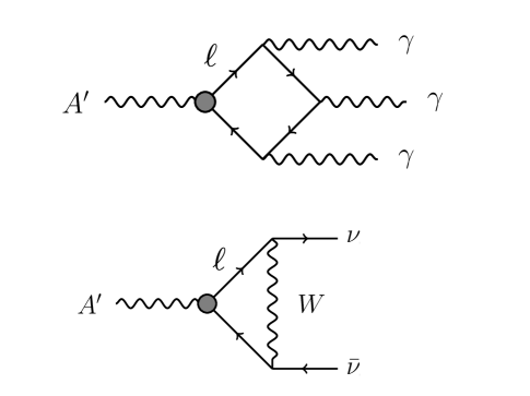
Figure 1: Feynman diagrams representing the $A^{\prime}\to 3\gamma$ (top) and the $A^{\prime}\to\bar{\nu}\nu$ decay (bottom) channels for $m_{A^{\prime}}<2m_{\ell}$. In both processes, the gray dot at the $A^{\prime}$-$\ell$ vertex is the magnetic dipole interaction from Eq. (1) for charged leptons $\ell=e,\mu,\tau$. There are corresponding diagrams involving quarks for which the electroweak loop yields decays to lighter quark flavors instead of neutrinos.

This paper is organized as follows: in Sec. II we describe the model, in Sec. III we calculate the $A^{\prime}$ abundance via freeze in, in Sec. IV we present structure formation limits, in Sec. V we explore the indirect detection constraints and future projections for this model, and in Sec. VI we offer some concluding remarks.

II Theory Overview

II.1 Model Description

We extend the SM with a hidden $U(1)_{H}$ group with corresponding gauge boson $A^{\prime}$, which doesn’t couple to any SM particles through renormalizable operators. The leading infrared interaction between $A^{\prime}$ and SM particles is taken to be a magnetic dipole coupling

$${\cal L}_{\rm int}=\frac{d_{f}}{2}F_{\mu\nu}^{\prime}\bar{f}\sigma^{\mu\nu}f~{},$$ (1)

where $f$ is a charged SM fermion, $d_{f}$ is the corresponding magnetic dipole moment, and $F^{\prime}_{\mu\nu}$ is the $A^{\prime}$ field strength tensor. Such an interaction can arise if the $U(1)_{H}$ is unbroken at high energies and heavy particles charged appropriately under $U(1)_{H}$ and the SM are integrated out at low energies. Since the magnetic dipole coupling is a dimension-5 operator, Eq. (1) is only valid at energy (or temperature) scales that satisfy $E\ll d_{f}^{-1}$.

If the $A^{\prime}$ is initially massless, any potential kinetic mixing between $U(1)_{H}$ and $U(1)_{Y}$ gauge bosons can be rotated away, so the operator in Eq. (1) can be the dominant interaction with SM particles Dobrescu (2005). However, for $A^{\prime}$ to be a viable dark matter candidate, it must acquire a mass at some lower energy scale, at which point kinetic mixing of the form $\frac{\epsilon}{2}F^{\mu\nu}F^{\prime}_{\mu\nu}$ can arise from loops of SM particles through their dipole interactions, where

$$\epsilon\sim\frac{ed_{f}m_{f}}{4\pi^{2}}\approx 2\times 10^{-15}\left(\frac{m_{f}}{m_{e}}\right)\left(\frac{d_{f}\cdot\rm GeV}{10^{-8}}\right)~{},$$ (2)

which is derived in Appendix VI. In Ref.Pospelov et al. (2008), it was found that vector freeze-in through kinetic mixing could account for the full DM abundance for $\epsilon\sim 10^{-11}-10^{-12}$ over the $\sim$ keV-MeV mass range. However, from Eq. (2), it is clear that the induced kinetic mixing can easily be subdominant to dipole production through the operator in Eq. (1); throughout this paper, we will only consider parameter space for which this requirement holds.

II.2 Leptonic Couplings

In this section we consider the decay channels that arise from coupling $A^{\prime}$ to charged leptons with $f=\ell$ in Eq. (1), where $\ell=e,\mu,\tau$ is the flavor of the dipole interaction. For $m_{A^{\prime}}>2m_{\ell}$, the dominant decay channel is $A^{\prime}\to\ell\bar{\ell}$, which is generically too prompt for the dark photon to serve as a viable dark matter candidate. However, for $m_{A^{\prime}}<2m_{\ell}$, the $A^{\prime}\to 3\gamma$ channel shown at the top of Fig. 1 can be cosmologically metastable due to phase-space suppression, so throughout this paper, we will only consider this mass ordering. In the $m_{A^{\prime}}\ll m_{\ell}$ limit, the $3\gamma$ decay width is

$$\Gamma_{A^{\prime}\to 3\gamma}=\frac{\alpha^{3}d_{\ell}^{2}m_{A^{\prime}}^{9}}{155520\,\pi^{4}m_{\ell}^{6}}~{},$$ (3)

which corresponds to a vector lifetime of

$$\tau_{A^{\prime}}\approx 10^{18}\,\text{Gyr}\left(\frac{10^{-10}\rm}{d_{\ell}\cdot\rm\,GeV}\right)^{2}\left(\frac{10\,\rm keV}{m_{A^{\prime}}}\right)^{9}\left(\frac{m_{\ell}}{m_{e}}\right)^{6}\!\!,~{}~{}~{}~{}~{}$$ (4)

so the $A^{\prime}$ can easily be metastable on cosmological timescales if there are no faster decay channels.

The $A^{\prime}$ can also decay to neutrinos through one-loop diagrams involving virtual $W$ exchange, as shown in the bottom of Fig. 1. The partial width for this process is

$$\Gamma_{A^{\prime}\to\bar{\nu}\nu}=\frac{d^{2}_{\ell}G_{F}^{2}m_{\ell}^{2}m_{A^{\prime}}^{5}}{4\pi^{3}}\log^{2}\!\left(\frac{m_{W}}{m_{\ell}}\right)~{},$$ (5)

and the ratio of partial widths satisfies

$$\frac{\Gamma_{A^{\prime}\to\bar{\nu}\nu}}{\Gamma_{A^{\prime}\to 3\gamma}} \approx 3\times 10^{-3}\left(\frac{m_{\ell}}{m_{e}}\right)^{8}\left(\frac{10\,\rm keV}{m_{A^{\prime}}}\right)^{4}~{},$$ (6)

where $G_{F}=1.16\times 10^{-2}$ GeV^-2 is the Fermi constant and we have set $m_{\ell}=m_{e}$ inside the log of Eq. (5). Since avoiding cosmologically prompt $A^{\prime}\to\bar{\ell}\ell$ decays requires $m_{A^{\prime}}<2m_{\ell}$, saturating this inequality maximizes the dominance of the photon channel

$$\frac{\Gamma_{A^{\prime}\to\bar{\nu}\nu}}{\Gamma_{A^{\prime}\to 3\gamma}}\approx 1.5\times 10^{-2}\left(\frac{m_{\ell}}{m_{\mu}}\right)^{4}\biggr{|}_{m_{A^{\prime}}=2m_{\ell}}~{}.$$ (7)

Thus, for $\ell=e$ or $\mu$ it is possible for the visible $3\gamma$ channel to dominate over the $A^{\prime}\to\bar{\nu}\nu$ channel while maintaining $m_{A^{\prime}}<2m_{\ell}$; for $\ell=\tau$ most $A^{\prime}$ decays are invisible, but there can still be a subdominant photon signal from the $3\gamma$ decay.

Note that for $m_{A^{\prime}}>2m_{\ell^{\prime}}$, where $\ell^{\prime}$ is a lighter lepton flavor, there are also model dependent $A^{\prime}\to{\ell^{\prime}}^{+}{\ell^{\prime}}^{-}$ decays induced by the kinetic mixing from Eq. (2), as shown in Fig. 2. The partial width for this process is

$$\Gamma_{A^{\prime}\to{\ell^{\prime}}^{+}{\ell^{\prime}}^{-}}=\frac{\epsilon^{2}\alpha m_{A^{\prime}}}{3}\left(1+\frac{2m^{2}_{\ell^{\prime}}}{m^{2}_{A^{\prime}}}\right)\sqrt{1-\frac{4m^{2}_{\ell^{\prime}}}{m^{2}_{A^{\prime}}}}~{}.$$ (8)

For $\ell=\mu$ and $\ell^{\prime}=e$, neglecting the phase space factors gives the ratio

$$\frac{\Gamma_{A^{\prime}\to{\ell^{\prime}}^{+}{\ell^{\prime}}^{-}}}{\Gamma_{A^{\prime}\to 3\gamma}}\approx 10^{10}\left(\frac{m_{\ell}}{m_{\mu}}\right)^{8}\left(\frac{50\,\rm MeV}{m_{A^{\prime}}}\right)^{8}~{},$$ (9)

so the kinetic mixing process is generically the dominant visible channel when kinetimatically accessible, and this can directly produce additional photons through final state radiation (FSR) via $A^{\prime}\to{\ell^{\prime}}^{+}{\ell^{\prime}}^{-}\gamma$ decays.

Although the total width properly includes the $3\gamma,\bar{\nu}\nu,$ and all available ${\ell^{\prime}}^{+}{\ell^{\prime}}^{-}$ channels, in our analysis, we treat the kinetic mixing scenario separately as the magnitude of this mixing can vary considerably depending on the full particle spectrum at high energies. In Figs. 3 and 4 we present our main results with and without kinetic mixing contributions, respectively (see Sec. V.2 and V.3 for details).

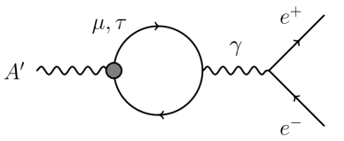
Figure 2: Example Feynman diagram for an $A^{\prime}\to e^{+}e^{-}$ decay through the induced kinetic mixing in Eq. (2). Although we only consider $m_{A^{\prime}}<2m_{\ell}$ so that $A^{\prime}\to\ell^{+}\ell^{-}$ decays are forbidden, these loop-level two-body decays can dominate over the $3\gamma$ channel for $m_{A^{\prime}}>2m_{e}$. Similarly $A^{\prime}\to\mu^{+}\mu^{-}$ decays can arise for $m_{A}^{\prime}>2m_{\mu}$ if $A^{\prime}$ has a dipole coupling to taus.

II.3 Hadronic Couplings

If the dipole in Eq. (1) involves SM quark fields and the vector mass is above the scale of QCD confinement, $m_{A^{\prime}}\gg\Lambda_{\rm QCD}\approx 200$ MeV, many of the qualitative features from the leptonic scenario in Sec. II.2 remain applicable. The key difference in the hadronic case is that the 2-body decay through a $W$ loop yields two lighter quarks instead of neutrinos, so this channel may be observable even if the $3\gamma$ decay is subdominant.

Since decay widths involving quark dipoles are parametrically similar to those involving leptons, the argument leading to Eq. (7) remains valid for this scenario. Thus, for $m_{A^{\prime}}<2m_{q}$ and $m_{A^{\prime}}>\Lambda_{\rm QCD}$, the loop level 2-body decay will be dominant for all quarks with masses above the confinement scale (i.e. $q=c,t,b$). However, for such heavier quark masses, it is generically difficult to ensure cosmological metastability for dipole couplings that can accommodate the observed dark matter abundance through freeze-in production (see Sec. III below). For example, using the loop induced 2-body width for $A^{\prime}\to d\bar{d}$ through a charm quark dipole, we have

$$\tau_{A^{\prime}}\approx 3\times 10^{10}\,{\rm yr}\,\left(\frac{10^{-14}}{d_{c}\cdot\rm\,GeV}\right)^{2}\left(\frac{m_{A^{\prime}}}{500\,\rm MeV}\right)^{5}~{},$$ (10)

where we have used the CKM matrix element $|V_{cd}|\approx 0.23$ Zyla et al. (2020) for the $c\to d$ transitions in the electroweak loop. Thus, even for dipole couplings with GUT scale suppression, the $A^{\prime}$ lifetime is typically short for cosmological metastabiltiy.

In principle, it should be possible to evade this conclusion in the $m_{A^{\prime}}\ll\Lambda_{\rm QCD}$ regime where the smaller mass suppresses the vector lifetime. However, in this scenario, the UV dipole coupling to quarks must be matched onto the confined theory, which is beyond the scope of this work, but deserves further attention. Thus, for the remainder of this paper, we will not consider quark dipole couplings in our numerical results.

III Cosmological Abundance

In this section we compute the $A^{\prime}$ abundance through freeze-in production. Since the dipole operator in Eq. (1) is not gauge invariant under $SU(2)_{L}\times U(1)_{Y}$, the dominant production processes will depend on whether the reheat temperature is above or below the scale of electroweak symmetry breaking, so we consider these cases separately.

Furthermore, since the dipole interaction is a higher dimension operator, the $A^{\prime}$ abundance is sensitive to the highest temperature achieved in the early universe and the production is most efficient at early times. Consequently, up to negligible corrections, the yields we calculate below are nearly identical for all lepton flavors and (up to color/charge factors) also apply to SM quarks if $T_{\rm RH}\gg\Lambda_{\rm QCD}$.

III.1 High Reheat Temperature $T_{\rm RH}>T_{\rm EW}$

In the early universe, at temperatures above the scale of electroweak symmetry breaking $T>T_{\rm EW}\approx 160$ GeV D’Onofrio and Rummukainen (2016), the operator in Eq. (1) must be evaluated in its electroweak preserving form

$${\cal L}_{\rm int}=\frac{d_{\ell}}{\sqrt{2}v}\,{\cal H}\,F^{\prime}_{\mu\nu}\bar{L}\sigma^{\mu\nu}\ell_{R},$$ (11)

where $\cal H$ is the Higgs doublet, $L$ is a lepton doublet of any generation, $\ell_{R}$ is the corresponding right handed fermion, and $v=246$ GeV is the Higgs vacuum expectation value. Assuming a negligible DM abundance at reheating, the $A^{\prime}$ population arises predominantly from pair annihilation $\ell^{+}\ell^{-}\to hA^{\prime}$ and Compton-like production $\ell h\to\ell A^{\prime}$ with corresponding cross sections

$$\sigma_{\ell^{+}\ell^{-}\to hA^{\prime}}=\frac{d_{\ell}^{2}s}{48\pi v^{2}}~{}~{},~{}~{}\sigma_{\ell h\to\ell A^{\prime}}=\frac{d_{\ell}^{2}s}{8\pi v^{2}}~{},~{}~{}~{}$$ (12)

where $s$ is the Mandelstam variable. Note that there are analogous processes involving the other doublet components related by $SU(2)_{L}$ invariance whose cross sections are equivalent to those in Eq. (12).

The thermally averaged cross section times velocity for these reactions can be written

$$\langle\sigma v\rangle=\frac{1}{32T^{5}}\int_{0}^{\infty}ds\,\sigma(s)s^{3/2}K_{1}\left(\frac{\sqrt{s}}{T}\right),$$ (13)

where $K_{1}$ is a modified Bessel function of the first kind and we have taken the massless limit of the analogous expression derived in Ref. Gondolo and Gelmini (1991).

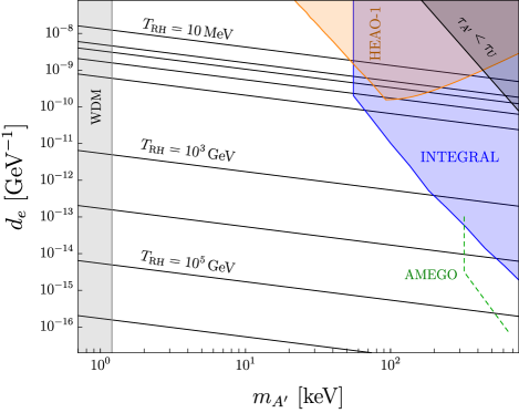
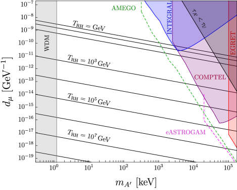
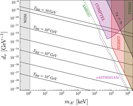
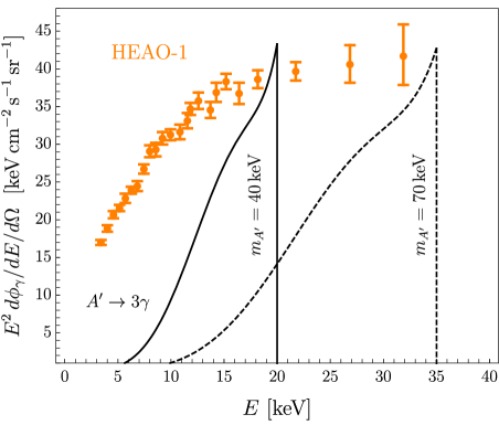
Figure 3: Top left: parameter space for which $A^{\prime}$ production via dipole freeze-in achieves the observed DM abundance for various values of reheat temperature (black contours); note that few MeV is excluded by the successful predictions of standard BBN. For higher values of reheat temperature, the abundance curves shift downwards by $\propto T^{3}_{\rm RH}$ from Eq. (16). Also shown are indirect detection limits on $A^{\prime}\to 3\gamma$ from EGRET Strong et al. (2004, 2003), Fermi Ackermann et al. (2012), COMPTEL Strong et al. (1994); Sreekumar et al. (1997), INTEGRAL Bouchet et al. (2008), and HEAO-1 Gruber et al. (1999), and structure formation limits on warm dark matter (WDM) (see Sec. IV). We show future projections from e-ASTROGAM Tavani et al. (2018) and AMEGO Kierans (2020) in dashed magenta and green curves, respectively. The top right and bottom left panels show the same parameter space, but for muon and tau couplings, respectively. Here we only include the $A^{\prime}\to 3\gamma$ channel and assume no (model dependent) contributions from kinetic mixing which induces $A^{\prime}\to e^{+}e^{-}\gamma,\mu^{+}\mu^{-}\gamma$ decays that yield additional signal photons (see Fig. 4 for these additional contributions). Also note that the reheat temperature is only evaluated above the SM lepton mass to ensure a relativstic population of such particles in the early universe. Bottom right: flux comparison between the HEAO-1 X-ray (orange data points) Lumb et al. (2002); De Luca and Molendi (2004); Nevalainen et al. (2005); Hickox and Markevitch (2006); Carter and Read (2007) and the predicted $A^{\prime}\to 3\gamma$ signal from Eq. (28). We also show representative signals for $m_{A^{\prime}}=40$ keV and $d_{e}=5.7\times 10^{-9}\,\rm GeV^{-1}$ (solid black) and $m_{A^{\prime}}=70$ keV with $d_{e}=4.6\times 10^{-10}\,\rm GeV^{-1}$ (dashed black).

In terms of the dimensionless yield $Y_{A^{\prime}}=n_{A^{\prime}}/{\cal S}$, where ${\cal S}=2\pi^{2}g_{\star,S}T^{3}/45$ is the entropy density and $g_{\star,S}$ is the number of entropic degrees of freedom, the Boltzmann equation for $A^{\prime}$ production can be written

$$\frac{dY_{A^{\prime}}}{dT}=-\frac{4n_{\ell}}{H{\cal S}T}\left[n_{\ell}\langle\sigma v\rangle_{\ell\ell\to hA^{\prime}}+2n_{h}\langle\sigma v\rangle_{\ell h\to\ell A^{\prime}}\right],~{}~{}~{}$$ (14)

where $T$ is the photon temperature, $H=1.66\sqrt{g_{\star}}T^{2}/m_{\rm Pl}$ is the Hubble rate, $g_{\star}$ is the effective number of relativistic species, $m_{\rm Pl}$ is the Planck mass, and $n_{\ell}=3\zeta(3)T^{3}/(2\pi^{2})$ and $n_{h}=\zeta(3)T^{3}/\pi^{2}$ are the electron and Higgs number densities in equilibrium; we have neglected terms corresponding to the reverse reactions ($A^{\prime}\ell\to h\ell$ etc.) due to the small relative $A^{\prime}$ abundance in the early universe. Note that the factor of 2 in the second term of Eq. (14) accounts for Compton-like $A^{\prime}$ production off both $\ell^{\pm}$ and the overall factor of 4 accounts for the multiplicity of states in the $\cal H$ doublet.

Since the dipole interaction is a higher dimension operator, the $A^{\prime}$ abundance is sensitive to the reheat temperature of the universe, $T_{\rm RH}$. Assuming instantaneous reheating and $g_{\star}=g_{\star,S}=$ constant throughout $A^{\prime}$ production, Eq. (14) can be integrated to obtain the asymptotic $A^{\prime}$ yield at late times

$$Y^{\infty}_{A^{\prime}}\approx 0.1\,\frac{d_{\ell}^{2}\,T^{3}_{\rm RH}m_{\rm Pl}}{g_{\star}^{3/2}v^{2}}~{}~{},$$ (15)

and the DM density fraction is $\Omega_{A^{\prime}}=m_{A^{\prime}}s_{0}Y_{A^{\prime}}^{\infty}/\rho_{c}$, where $s_{0}=2.1\times 10^{-38}$ GeV³ is the present day entropy density and $\rho_{c}=4.1\times 10^{-47}$ GeV⁴ is the critical density. Obtaining the observed DM abundance requires an overall normalization

$$\Omega_{A^{\prime}} \approx \Omega_{\rm DM}\left(\frac{m_{A^{\prime}}}{3\,\rm MeV}\right)\left(\frac{d_{\ell}\cdot\rm GeV}{10^{-13}}\right)^{2}\left(\frac{T_{\rm RH}}{\rm TeV}\right)^{3}\!,~{}~{}~{}$$ (16)

which gives an adequate order of magnitude estimate. To obtain our final results, we numerically integrate Eq. (14) to calculate $Y_{A^{\prime}}^{\infty}$. Note that our derivation is equally applicable to any lepton $\ell$ since the abundance is UV dominated and insensitive to the low-energy fermion mass for all $T_{\rm RH}>T_{\rm EW}$.

Note that in the presence of nonzero kinetic mixing, there are additional production channels through $f\bar{f}\to A^{\prime}$ inverse decays, which can modify the cosmological $A^{\prime}$ abundance. However, we have verified that including this channel (and other production modes that depend on the kinetic mixing), only contributes negligibly to the late time yield if the mixing arises from the dipole operator as in Eq. (2).

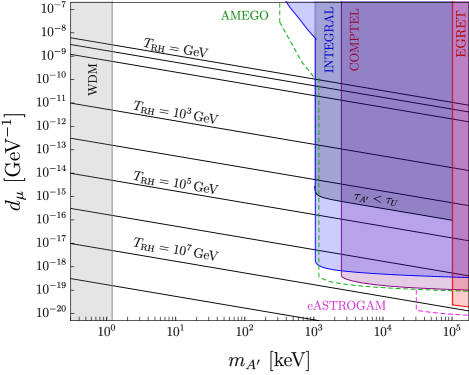
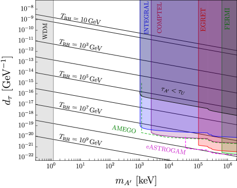
Figure 4: Same as the corresponding panels in Fig. 3, but including the effect of kinetic mixing for the muon and tau flavor dipole couplings. Here the indirect detection signals are significantly affected by additional photons from $A^{\prime}\to{\ell^{\prime}}^{+}{\ell^{\prime}}^{-}\gamma$ reactions where $\ell^{\prime}$, is a lighter lepton flavor than the tree-level dipole coupling to flavor $\ell$

III.2 Low Reheat Temperature $T_{\rm RH}<T_{\rm EW}$

If the reheat temperature is below the electroweak scale, the Higgs doublet is set to its vacuum expectation value $\langle H\rangle=v/\sqrt{2}$ and Eq. (11) recovers Eq. (1). In this regime, the leading freeze-in reactions are $\ell^{+}\ell^{-}\to\gamma A^{\prime}$ and $\ell^{\pm}\gamma\to\ell^{\pm}A^{\prime}$ with respective cross sections

$$\sigma_{\ell\gamma\to\ell A^{\prime}}=\frac{\alpha d_{\ell}^{2}}{2}~{},~{}~{}~{}\sigma_{\ell^{+}\ell^{-}\to\gamma A^{\prime}}=\alpha d_{\ell}^{2}~{}~{},~{}~{}$$ (17)

where $\alpha$ is the fine structure constant. The Boltzmann equation for $A^{\prime}$ production now becomes

$$\frac{dY_{A^{\prime}}}{dT}=-\frac{n_{\ell}}{H{\cal S}T}\left[n_{\ell}\langle\sigma v\rangle_{\ell\ell\to\gamma A^{\prime}}+2n_{\gamma}\langle\sigma v\rangle_{\ell\gamma\to\ell A^{\prime}}\right],~{}~{}~{}$$ (18)

where $n_{\gamma}=2\zeta(2)T^{3}/\pi^{2}$ is the photon number density in equilibrium and the thermal averages are trivial since the cross sections in Eq. (17) are constant for $T_{\rm RH}\ll d_{\ell}^{-1}$, so $\langle\sigma v\rangle\approx\sigma$ for these processes. Integrating Eq. (18) from $T_{\rm RH}\to m_{\ell}$ and approximating $g_{\star}=g_{\star,S}=$ constant, the asymptotic yield is

$$Y_{A^{\prime}}^{\infty}\approx 0.1\,\alpha g_{\star}^{-3/2}d_{\ell}^{2}T_{\rm RH}\,m_{\rm Pl}~{}~{},$$ (19)

which corresponds to a present-day dark matter abundance of

$$\Omega_{A^{\prime}}\approx\Omega_{\rm DM}\left(\frac{d_{\ell}\cdot\rm GeV}{10^{-10}}\right)^{2}\left(\frac{m_{A^{\prime}}}{\rm MeV}\right)\left(\frac{T_{\rm RH}}{\rm GeV}\right),$$ (20)

where we have evaluated $g_{\star}$ at $T_{\rm RH}$. In our numerical results, we integrate the full expression in Eq. (18) to compute $A^{\prime}$ the abundance.

III.3 Inflationary Production

In addition to the freeze-in abundance computed above, if the $A^{\prime}$ has a nonzero mass during inflation, there is also an irreducible vector population produced through inflationary fluctuations Graham et al. (2016)

$$\Omega_{A^{\prime}}^{\rm inf}\approx\Omega_{\rm DM}\sqrt{\frac{m_{A^{\prime}}}{6\,\mu\rm eV}}\left(\frac{H_{I}}{10^{14}\,\rm GeV}\right)^{2}~{},$$ (21)

where $H_{I}$ is the Hubble rate during inflation. In our scenario, the minimum Hubble rate during inflation satisfies $H_{I,\rm min}\sim T_{\rm RH}^{2}/m_{\rm Pl}$, corresponding to an instantaneous transfer of energy from the inflaton to the SM radiation bath, so the minimum $A^{\prime}$ abundance from inflationary production is

$$\Omega^{\rm min}_{A^{\prime}}\approx 10^{-19}\sqrt{\frac{m_{A^{\prime}}}{\rm MeV}}\left(\frac{T_{\rm RH}}{10^{10}\,\rm GeV}\right)^{4}~{},$$ (22)

which is negligible across our entire parameter space of interest. Thus, assuming instantaneous reheating, if $T_{\rm RH}$ is sufficiently large for a non-trivial inflationary abundance, freeze-in production from Eq. (16) generically overcloses the universe.

If there is a large hierarchy between $H_{I}$ and $T_{\rm RH}$ (e.g. due an alternative cosmic expansion history Allahverdi et al. (2020)), then freeze-in production can be subdominant to inflationary production. However, independently of $T_{\rm RH}$, generating a non-trivial abundance generically requires a large value of $H_{I}\sim 10^{14}$ GeV, in some tension with Planck limits on primordial tensor modes in CMB data Aghanim et al. (2020). Thus, for the remainder of this work, we remain agnostic about the value of $H_{I}$ and neglect any possible contribution from inflationary production, but it might be interesting to explore the full parameter space of such a hybrid scenario in future work.

IV Structure Formation

In our scenario, the $A^{\prime}$ population is mainly produced relativistically through freeze-in at high temperatures, near $T_{\text{RH}}$. For low values of $m_{A^{\prime}}\sim$ keV, its phase space distribution can be warm at late times and erase small scale cosmological structure in conflict with various structure formation probes, including gravitational lensing, the Ly-alpha forest, and the inventory of dwarf satellites in the Milky Way, among others.

Constraints on warm dark matter (WDM) are typically calculated for thermal relics and assume that all of the DM inherited a thermal velocity distribution at freeze out, in analogy with relic neutrinos. Such constraints can also be applied to feebly interacting DM particles that were never in equilibrium, but produced instead via freeze-in if their velocity distribution has a nearly thermal profile. This is the case when the reaction rate is maximal near the freeze-in temperature $T_{\text{FI}}$ at which most DM particles are produced. In our scenario, this production is dominated by reactions at $T_{\text{FI}}\sim T_{\text{RH}}$, as discussed in Sec. III.

For WDM with a thermal spectrum, the constraint from structure formation can be calculated using the free streaming length

$$\ell_{\text{FS}}\equiv\int_{z_{f}}^{z_{i}}v(z)\frac{dz}{H(z)},\quad v(z)=\frac{p(z)}{\sqrt{m^{2}+p^{2}(z)}},$$ (23)

where $v(z)$ is the particle velocity, $p_{i}$ is its momentum at initial redshift $z_{i}$, and we have defined

$$p(z)\equiv\left(\frac{1+z}{1+z_{i}}\right)p_{i}~{}.$$ (24)

Note that $\ell_{\rm FS}$ a monotonically growing function of $p_{\text{com}}/m$, where

$$p_{\text{com}}=\frac{p_{i}}{1+z_{i}}~{},$$ (25)

is the comoving momentum of the particle, so the physical constraint on $\ell_{\text{FS}}$ can be translated into a constraint on the quantity

$$\frac{p_{\text{com}}}{m}=\frac{p_{i}}{m(1+z_{i})}\sim\frac{T_{\text{FI}}}{m(1+z_{i})}~{},$$ (26)

where $m$ is the mass of a thermal WDM candidate. In the absence of any entropy transfers into the primordial plasma, the quantity $T_{\text{FI}}/(1+z_{i})$ is constant and therefore, $\ell_{\rm FS}$ can be used to directly constrain the mass of the DM particle. However, since our scenario is sensitive to potentially high values of the reheat temperature, all entropy transfers at $T<T_{\rm RH}$ must be taken into account in order to translate $\ell_{\text{FS}}$ into a limit on the DM mass. Using entropy conservation, the $T/(1+z)$ ratio for our scenario relative to that of thermal WDM is given by

$$\frac{T_{A^{\prime}}}{T_{\text{relic}}}\left(\frac{1+z_{\text{relic}}}{1+z_{A^{\prime}}}\right)=\left[\frac{g_{\star}(T_{\text{ relic}})}{g_{\star}(T_{\text{RH}})}\right]^{1/3}~{},$$ (27)

where $z_{\rm relic}$ is the redshift at which a thermal relic freezes out; this ratio be used to translate conventional WDM bounds into a lower limits on our dark photon mass.

In the literature (see e.g.Zelko et al. (2022) and refs therein), there are many different constraints on the mass of the thermal relic WDM particles extracted using different analysis methods. Such studies typically assume that DM freezes decouples from the SM at $T_{\text{relic}}^{\text{th}}\sim 2\text{ MeV}$, so $g_{\star}(T_{\text{relic}}^{\text{th}})=10.75$. However, our dark photons are produced at $T_{\text{RH}}$ and if we take $g_{\star}(T_{\text{RH}})=106.75$ – the total number of relativistic SM degrees of freedom at high temperature – we conclude that for the same $\ell_{\text{FS}}$, the analogous constraint on the dark photon mass is approximately $(106.75/10.75)^{1/3}\approx 2.15$ times weaker than traditionally reported limits on WDM thermal relics.

Although there are many such WDM limits in the literature (see Ref. Iršič et al. (2017) for a discussion), we place conservative limits on our scenario using the weakest bounds from Ref. Garzilli et al. (2019) which constrains $m_{\rm WDM}>2.5$ keV by considering a wider class of viable reionization models relative to other analyses. Translating this limit into a bound on our scenario resuts in a constraint of $m_{A^{\prime}}>1.2$ keV. Note that this bound can be further relaxed if new particles with masses below $T_{\text{RH}}$ are thermalized in the early universe and provide additional entropy transfers into the SM radiation bath, resulting in a larger value of $g_{\star}(T_{\text{RH}})$.

V Indirect Detection

V.1 General Formalism

The differential photon flux from decaying DM in our our Galaxy is given by

$$\frac{d\phi_{\gamma}}{dEd\Omega}=\frac{r_{\odot}}{4\pi}\frac{\rho_{\odot}\Gamma}{m_{A^{\prime}}}\frac{dN_{\gamma}}{dE}D,$$ (28)

where $r_{\odot}=8.5$ kpc is the solar distance from the Galactic center, $\rho_{\odot}=0.3\text{ GeV}\text{cm}^{-3}$ is the local DM density, and $D$-factor is defined according to

$$D\equiv\int_{l(\Omega)}\frac{dl}{r_{\odot}}\frac{\rho(l,\Omega)}{\rho_{\odot}}~{},$$ (29)

where the line integral is over the observed line of sight $l(\Omega)$ for a given solid angle $\Omega$. For the 3$\gamma$ decay channel, the inclusive single-photon spectrum is

$$~{}~{}\frac{d\Gamma}{dE}=\dfrac{\alpha^{3}d_{\ell}^{2}m_{A^{\prime}}^{3}E^{3}}{9720\,\pi^{4}m_{\ell}^{6}}\left(35m_{A^{\prime}}^{2}-130Em_{A^{\prime}}+126E^{2}\right)\!,~{}~{}~{}~{}~{}~{}~{}$$ (30)

where $E\leq m_{A^{\prime}}/2$ and the differential photon spectrum from three body decays is

$$\frac{dN_{\gamma}}{dE}=\frac{3}{\Gamma}\frac{d\Gamma}{dE}~{},$$ (31)

where the factor of 3 accounts for the photon yield per decay event. Inserting this result into Eq. (28) alongside Eq. (3) yields our photon flux in terms of model parameters.

When the kinetic mixing in Eq. (2) is nonzero, for masses $m_{A^{\prime}}>2m_{\ell^{\prime}}$, there are also $A^{\prime}\to{\ell^{\prime}}^{+}{\ell^{\prime}}^{-}$ decays, where ${\ell^{\prime}}$ is a fermionic species lighter than $\ell$, the original dipole flavor as depicted in Fig. 2. These charged particles can yield potentially observable secondary photons via synchrotron radiation and inverse Compton scattering; such decays can also yield excesses in the cosmic positron spectrum. There are a number of works dedicated to constraining DM annihilation and decays into charged particles Ibarra et al. (2010); Boudaud et al. (2017); Gaggero and Valli (2018); Moskalenko and Strong (1999); Boudaud et al. (2019). However, in this work, we do not include this analysis. Instead, we present the conservative bounds from quantum corrections to the radiative tree-level process $A^{\prime}\to{\ell^{\prime}}^{+}{\ell^{\prime}}^{-}\gamma$ with an additional photon through FSR. The photon spectrum for this process can be written Siegert et al. (2022)

$$~{}~{}\frac{dN_{\gamma}}{dE}\simeq\frac{\alpha[m_{A^{\prime}}^{2}+(m_{A^{\prime}}-2E)^{2}]}{2\pi\,m_{A^{\prime}}^{2}E}\log\left(\frac{m_{A^{\prime}}(m_{A^{\prime}}-2E)}{m_{\ell}^{2}}\right),~{}~{}~{}~{}~{}~{}$$ (32)

which arises by integrating the Altarelli-Parisi splitting function with a $\delta-$function.

V.2 Analysis Method

In this section we place limits on the signal from Eq. (28) using observations of the diffuse X-ray background from the HEAO-1 Gruber et al. (1999), INTEGRAL Bouchet et al. (2008), COMPTEL Strong et al. (1994); Sreekumar et al. (1997), EGRET Strong et al. (2004, 2003) and Fermi Ackermann et al. (2012) instruments. After removing known point sources from each data set, the resulting X-ray spectrum consists of three components: Galactic emission, instrumental backgrounds, and the diffuse X-ray background (XRB). Since the Galactic and instrumental components contain a large number of spectral lines from atomic transitions, properly extracting the diffuse emission from the full spectrum requires a model of all relevant atomic lines and several additional power-law components. To properly constrain a DM decay signal using this diffuse emission, such modeling must be repeated in the presence of the additional DM induced spectral component, which is beyond the scope of this work.

Instead, to extract a conservative, order of magnitude constraint from these instruments, we use the observational data shown in Fig. 5 and, for each choice of DM mass, we demand that the number of signal photons in each bin does not exceed the number predicted by the XRB central value by more than two statistical standard deviations, except for the EGRET and Fermi, where the dominant systematic uncertainties are taken (see Ref. Essig et al. (2013) for a discussion of this approach). For the data sets we use Galactic $D$-factors computed in Ref. Essig et al. (2013), which assumes a Navarro-Frenk-White DM profile Navarro et al. (1996), and our results for different $A^{\prime}$ lepton dipole couplings are presented in Fig 3. In principle, the XMM-Newton telescope Carter and Read (2007) can also be used to constrain this model, but we have verified that this limit corresponds to parameter space for which the freeze-in density can only be achieved for $T_{\rm RH}\ll$ MeV, which is not shown in Fig. 5.

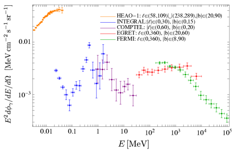
Figure 5: Observed X-ray flux data sets used to constrain the $A^{\prime}\to 3\gamma$ signal in this scenario – figure adapted from Ref. Essig et al. (2013). Here the $\ell$ and $b$ values represent longitude and latitude coordinates within each instrument’s field of view. Note that each instrument observes a different region of the sky, so the data sets presented here should not be compared against each other.

V.3 Future Projections

In this section we compute projections for future missions with sensitivity to the $A^{\prime}\to 3\gamma$ and $A^{\prime}\to{\ell^{\prime}}^{+}{\ell^{\prime}}^{-}\gamma$ decay channels. We consider the next generation X-ray telescope Athena alongside MeV telescopes e-ASTROGAM Tavani et al. (2018) and AMEGO Kierans (2020), which can improve sensitivity to our decay signature. Collectively, these future probes will have improved energy resolution, larger effective area, and wider fields of view, which serve to reduce astrophysical uncertainties in the background and improve signal reach.

To model the sensitivity of these instruments, we bin our predicted signal in units of the reported energy resolution for each telescope and demand that the visible DM decay signal not exceed the statistical uncertainty on the photon background. Thus, for a minimal detectable flux in the $i^{\text{th}}$ energy bin, demanding 2$\sigma$ sensitivity, $N_{\text{signal}}=2\sqrt{N_{\text{bg}}}$, yields

$$\int_{E_{\min,i}}^{E_{\max,i}}\frac{d\phi_{\text{signal}}}{dE}dE=2\sqrt{\frac{d\phi_{\text{bg}}}{dE}\frac{\Delta E}{A_{\rm eff}\Delta t_{\rm obs}}}~{}~{},$$ (33)

where $\Delta t_{\rm obs}$ is the observation time, $A_{\rm eff}(E)$ is the instrument’s effective area, $\Delta E$ is the energy resolution, $d\phi_{\text{bg}}/dE$ is the background flux, and we integrate the signal over the energy range $(E_{\min,i},E_{\max,i})$ spanned by the bin.

For our background flux estimates, we adopt XMM-Newton’s models to compute Athena projections, COMPTEL and EGRET for e-ASTROGAM, and INTEGRAL, COMPTEL, EGRET and Fermi as proxies for our AMEGO projections. To calculate the relevant $D$-factor, we need to know the spatial orientations of these future telescopes, which are not yet finalized. Thus, for Athena, we use the average $D$-factor of the XMM-Newton blank sky background and re-scale for Athena’s larger projected field of view. For e-ASTROGAM and AMEGO, we similarly re-scale the $D$-factors from INTEGRAL, COMPTEL, EGRET and Fermi correspondingly. In Fig. 3 we present our results including sensitivity projections for e-ASTROGAM and AMEGO; we find that Athena is only sensitive to dipole values which require $T_{\rm RH}\ll$ MeV to yield the observed freeze-in abundance, so its projections are not shown in Figs. 3 and 4.

VI Conclusion

In this paper we introduced a simple model of vector DM with feeble magnetic dipole couplings to charged SM particles. In the early universe, the DM is produced non-thermally through freeze-in and the present day abundance is sensitive to the reheat temperature, with different scaling before and after the electroweak phase transition.

If the vector mass is below the kinematic threshold for tree-level decays through the dipole coupling, loop level decays are generically suppressed either by phase space (for $A^{\prime}\to 3\gamma$) or by the $W$ mass for induced decays to lighter fermion species (e.g. $A^{\prime}\to\bar{\nu}\nu)$. Thus, for $m_{A^{\prime}}<2m_{f}$ and dipole couplings that yield the observed DM abundance, the vector is generically metastable on cosmological timescales. If loop-induced kinetic mixing is also included, then for $m_{A^{\prime}}>2m_{e}$ there are additional DM decay channels to pairs of charged particles throguh the electromagnetic current.

For tree-level dipole couplings to leptons, the loop induced $A^{\prime}\to 3\gamma$ decay and kinetic-mixing induced $A^{\prime}\to e^{+}e^{-}\gamma,\mu^{+}\mu^{-}\gamma$ decays predict visible photon signatures in the few-keV – few-GeV energy range, where the lower limit is set by structure formation limits on WDM and the upper limit is set by the requirement that $m_{A^{\prime}}<2m_{\tau}$ to avoid cosmologically prompt $A^{\prime}\to\tau^{+}\tau^{-}$ decays if the $A^{\prime}$ couples directly to taus. In this mass range, we have considered various observational constraints and computed projections for future missions including the Athena, e-ASTROGAM, and AMEGO telescopes, which will improve sensitivity to parameter space that yields the observed DM abundance through freeze-in for various values of reheat temperature.

Although we have studied various indirect detection probes for our scenario, we note that there are several directions available for future work:

• Charged Particle Decays: In the presence of nonzero kinetic mixing, the dominant decay channel for our DM candidate is $A^{\prime}\to f^{+}f^{-}$, whenever this is kinematically available. In our indirect detection analysis, we included signals from photons produced as FSR via $A^{\prime}\to f^{+}f^{-}\gamma$, but neglected the possibility of secondary photons from the more common $A^{\prime}\to f^{+}f^{-}$ process, which can yield additional detection handles from synchrotron radiation, inverse compton scattering, and antiparticle production. However, these channels require dedicated modeling of astrophysical environments to extract signal predictions, which is beyond the scope of this paper.

• Quark Couplings: If $A^{\prime}$ couples to quarks and $m_{A^{\prime}}>\Lambda_{\rm QCD}$, its lifetime is generically prompt for dipole couplings that can produce the observed DM abundance. For lighter $m_{A^{\prime}}<\Lambda_{\rm QCD}$ it may be possible for a quark-coupled $A^{\prime}$ to be a viable DM candidate, but investigating this mass range requires matching the $A^{\prime}$-quark dipole operator onto corresponding hadronic interactions below the QCD confinement scale, which we leave for future work.

• Direct Detection: Finally, we note that this model may be testable at low mass direct detection experiments via $A^{\prime}$ absorption onto detector targets, in analogy with searches for kinetically-mixed dark photon and axion-like dark matter candidates. Performing such a study would require a reanalysis of existing bounds and future reach projections using a matrix element for the dipole operator in Eq. (1), which we also leave for future work.

Appendix A Induced Kinetic Mixing

The dipole coupling in Eq. (1) induces a kinetic mixing interaction between the dark and visible photon. At some high energy scale $\Lambda$ in the theory, the kinetic mixing amplitude is identically zero. This requires us to introduce the renormalization condition

$$\Pi^{\mu\nu}(k^{2}\to\Lambda^{2})=0~{}~{},$$ (34)

where $k$ is the momentum associated with this diagram. The leading order contribution to kinetic mixing can be written

$$i\Pi^{\mu\nu} = ied_{f}k_{\rho}\int\frac{d^{4}p}{(2\pi)^{4}}\frac{\text{Tr}\Big{[}\sigma^{\mu\rho}(\not{p}-\not{k}+m_{f})\gamma^{\nu}(\not{p}+m_{f})\Big{]}}{[(p-k)^{2}-m_{f}^{2}][p^{2}-m_{f}^{2}]},$$

so using dimensional regularization and the modified minimal subtraction scheme, this integral becomes

$$i\Pi^{\mu\nu}=\frac{ied_{f}m_{f}}{(4\pi)^{2}}\left(k^{2}g^{\mu\nu}-k^{\mu}k^{\nu}\right)\int_{0}^{1}dx\log\left[\frac{m_{f}^{2}-x(1-x)k^{2}}{m_{f}^{2}-x(1-x)\Lambda^{2}}\right]~{}.$$

In the limit $\Lambda^{2}\gg m_{f}^{2},k^{2}$, this integral takes the form

$$i\Pi^{\mu\nu} =\frac{ied_{f}m_{f}}{8\pi^{2}}\left(k^{2}g^{\mu\nu}-k^{\mu}k^{\nu}\right)\log\Big{(}\frac{m_{f}^{2}}{\Lambda^{2}}\Big{)}$$ (35)

In order to express as an effective kinetic mixing coupling $\frac{\epsilon}{2}F^{\mu\nu}F^{\prime}_{\mu\nu}$, we simply remove the projector to obtain ,

$$\epsilon=\frac{ed_{f}m_{f}}{4\pi^{2}}\log\left(\frac{m_{f}^{2}}{\Lambda^{2}}\right)~{},$$ (36)

which justifies the approximate form presented in Eq. (2).

References

- Bertone and Hooper (2018) G. Bertone and D. Hooper, Rev. Mod. Phys. 90, 045002 (2018), arXiv:1605.04909 [astro-ph.CO] .
- Dodelson and Widrow (1994) S. Dodelson and L. M. Widrow, Phys. Rev. Lett. 72, 17 (1994), arXiv:hep-ph/9303287 .
- Hall et al. (2010) L. J. Hall, K. Jedamzik, J. March-Russell, and S. M. West, JHEP 03, 080 (2010), arXiv:0911.1120 [hep-ph] .
- Pospelov et al. (2008) M. Pospelov, A. Ritz, and M. Voloshin, Physical Review D 78 (2008), 10.1103/physrevd.78.115012.
- An et al. (2015) H. An, M. Pospelov, J. Pradler, and A. Ritz, Phys. Lett. B 747, 331 (2015), arXiv:1412.8378 [hep-ph] .
- Dobrescu (2005) B. A. Dobrescu, Physical Review Letters 94 (2005), 10.1103/physrevlett.94.151802.
- Zyla et al. (2020) P. A. Zyla et al. (Particle Data Group), PTEP 2020, 083C01 (2020).
- D’Onofrio and Rummukainen (2016) M. D’Onofrio and K. Rummukainen, Phys. Rev. D 93, 025003 (2016), arXiv:1508.07161 [hep-ph] .
- Gondolo and Gelmini (1991) P. Gondolo and G. Gelmini, Nucl. Phys. B 360, 145 (1991).
- Strong et al. (2004) A. W. Strong, I. V. Moskalenko, and O. Reimer, Astrophys. J. 613, 962 (2004), arXiv:astro-ph/0406254 .
- Strong et al. (2003) A. W. Strong, I. V. Moskalenko, and O. Reimer, in 28th International Cosmic Ray Conference (2003) pp. 2309–2312, arXiv:astro-ph/0306346 .
- Ackermann et al. (2012) M. Ackermann et al. (Fermi-LAT), Astrophys. J. 750, 3 (2012), arXiv:1202.4039 [astro-ph.HE] .
- Strong et al. (1994) A. W. Strong, K. Bennett, H. Bloemen, R. Diehl, W. Hermsen, D. Morris, V. Schoenfelder, J. G. Stacy, C. de Vries, M. Varendorff, C. Winkler, and G. Youssefi, A&A 292, 82 (1994).
- Sreekumar et al. (1997) P. Sreekumar, F. W. Stecker, and S. C. Kappadath, AIP Conf. Proc. 410, 344 (1997), arXiv:astro-ph/9709258 .
- Bouchet et al. (2008) L. Bouchet, E. Jourdain, J. P. Roques, A. Strong, R. Diehl, F. Lebrun, and R. Terrier, Astrophys. J. 679, 1315 (2008), arXiv:0801.2086 [astro-ph] .
- Gruber et al. (1999) D. E. Gruber, J. L. Matteson, L. E. Peterson, and G. V. Jung, Astrophys. J. 520, 124 (1999), arXiv:astro-ph/9903492 .
- Tavani et al. (2018) M. Tavani et al. (e-ASTROGAM), JHEAp 19, 1 (2018), arXiv:1711.01265 [astro-ph.HE] .
- Kierans (2020) C. A. Kierans (AMEGO Team), Proc. SPIE Int. Soc. Opt. Eng. 11444, 1144431 (2020), arXiv:2101.03105 [astro-ph.IM] .
- Lumb et al. (2002) D. H. Lumb, R. S. Warwick, M. Page, and A. De Luca, Astron. Astrophys. 389, 93 (2002), arXiv:astro-ph/0204147 .
- De Luca and Molendi (2004) A. De Luca and S. Molendi, Astron. Astrophys. 419, 837 (2004), arXiv:astro-ph/0311538 .
- Nevalainen et al. (2005) J. Nevalainen, M. Markevitch, and D. Lumb, Astrophys. J. 629, 172 (2005), arXiv:astro-ph/0504362 .
- Hickox and Markevitch (2006) R. C. Hickox and M. Markevitch, Astrophys. J. 645, 95 (2006), arXiv:astro-ph/0512542 .
- Carter and Read (2007) J. A. Carter and A. M. Read, Astron. Astrophys. 464, 1155 (2007), arXiv:astro-ph/0701209 .
- Graham et al. (2016) P. W. Graham, J. Mardon, and S. Rajendran, Phys. Rev. D 93, 103520 (2016), arXiv:1504.02102 [hep-ph] .
- Allahverdi et al. (2020) R. Allahverdi et al., (2020), 10.21105/astro.2006.16182, arXiv:2006.16182 [astro-ph.CO] .
- Aghanim et al. (2020) N. Aghanim et al. (Planck), Astron. Astrophys. 641, A6 (2020), [Erratum: Astron.Astrophys. 652, C4 (2021)], arXiv:1807.06209 [astro-ph.CO] .
- Zelko et al. (2022) I. A. Zelko, T. Treu, K. N. Abazajian, D. Gilman, A. J. Benson, S. Birrer, A. M. Nierenberg, and A. Kusenko, (2022), arXiv:2205.09777 [hep-ph] .
- Iršič et al. (2017) V. Iršič et al., Phys. Rev. D 96, 023522 (2017), arXiv:1702.01764 [astro-ph.CO] .
- Garzilli et al. (2019) A. Garzilli, A. Magalich, T. Theuns, C. S. Frenk, C. Weniger, O. Ruchayskiy, and A. Boyarsky, Mon. Not. Roy. Astron. Soc. 489, 3456 (2019), arXiv:1809.06585 [astro-ph.CO] .
- Ibarra et al. (2010) A. Ibarra, D. Tran, and C. Weniger, JCAP 01, 009 (2010), arXiv:0906.1571 [hep-ph] .
- Boudaud et al. (2017) M. Boudaud, J. Lavalle, and P. Salati, Phys. Rev. Lett. 119, 021103 (2017), arXiv:1612.07698 [astro-ph.HE] .
- Gaggero and Valli (2018) D. Gaggero and M. Valli, Adv. High Energy Phys. 2018, 3010514 (2018), arXiv:1802.00636 [astro-ph.HE] .
- Moskalenko and Strong (1999) I. V. Moskalenko and A. W. Strong, in 26th International Cosmic Ray Conference (1999) arXiv:astro-ph/9906230 .
- Boudaud et al. (2019) M. Boudaud, T. Lacroix, M. Stref, and J. Lavalle, Phys. Rev. D 99, 061302 (2019), arXiv:1810.01680 [astro-ph.HE] .
- Siegert et al. (2022) T. Siegert, C. Boehm, F. Calore, R. Diehl, M. G. H. Krause, P. D. Serpico, and A. C. Vincent, Mon. Not. Roy. Astron. Soc. 511, 914 (2022), arXiv:2109.03791 [astro-ph.HE] .
- Essig et al. (2013) R. Essig, E. Kuflik, S. D. McDermott, T. Volansky, and K. M. Zurek, JHEP 11, 193 (2013), arXiv:1309.4091 [hep-ph] .
- Navarro et al. (1996) J. F. Navarro, C. S. Frenk, and S. D. M. White, Astrophys. J. 462, 563 (1996), arXiv:astro-ph/9508025 .