Connecting Solar and Stellar Flares/CMEs: Expanding Heliophysics
to Encompass Exoplanetary Space Weather

Abstract

The aim of this white paper is to briefly summarize some of the outstanding gaps in the observations and modeling of stellar flares, CMEs, and exoplanetary space weather, and to discuss how the theoretical and computational tools and methods that have been developed in heliophysics can play a critical role in meeting these challenges. The maturity of data-inspired and data-constrained modeling of the Sun-to-Earth space weather chain provides a natural starting point for the development of new, multidisciplinary research and applications to other stars and their exoplanetary systems. Here we present recommendations for future solar CME research to further advance stellar flare and CME studies. These recommendations will require institutional and funding agency support for both fundamental research (e.g. theoretical considerations and idealized eruptive flare/CME numerical modeling) and applied research (e.g. data inspired/constrained modeling and estimating exoplanetary space weather impacts). In short, we recommend continued and expanded support for: (1.) Theoretical and numerical studies of CME initiation and low coronal evolution, including confinement of “failed” eruptions; (2.) Systematic analyses of Sun-as-a-star observations to develop and improve stellar CME detection techniques and alternatives; (3.) Improvements in data-inspired and data-constrained MHD modeling of solar CMEs and their application to stellar systems; and (4.) Encouraging comprehensive solar–stellar research collaborations and conferences through new interdisciplinary and multi-agency/division funding mechanisms.

1 Introduction

The aim of this white paper is to discuss the importance of both fundamental and applied coronal mass ejection (CME) research in the context of its increasing relevance to stellar astronomy. Interest in detecting and modeling CMEs on other stars has increased dramatically in recent years. The winds and CMEs of coronal stars like the Sun have always been of interest due to their role in shedding angular momentum, leading to observed declines in stellar rotation and activity with age [Vidotto, 2021]. However, by far the primary driver of interest in stellar winds and CMEs these days relates to star–planet interactions and the “space weather” impacts on exoplanetary atmospheres [Airapetian et al., 2020, and references therein].

As of March 2022, there are over 5000 confirmed exoplanet discoveries [Brennan, 2022]. Most of the known exoplanets orbit very close to their parent stars, meaning they are potentially exposed to particularly high particle fluxes from stellar winds to CMEs, leading to much interest in the long-term effects this exposure has on the atmospheres of these planets. Absorption from material evaporating from planetary atmospheres has actually been detected in cases of transiting exoplanets, indicating the importance of this process [Vidal-Madjar et al., 2003; Lecavelier Des Etangs et al., 2010; Ekenbäck et al., 2010; Kislyakova et al., 2014; Bourrier et al., 2016; Schneiter et al., 2016]. In our own solar system, solar wind and CME exposure may have significantly affected planetary atmospheric evolution, with Mars being a particularly interesting case [Jakosky et al., 2018].

Solar and stellar flares—sudden explosive releases of energy in the solar/stellar atmosphere across a wide range of electromagnetic wavelengths—occur due to the rapid release of free magnetic energy stored in the sheared and/or twisted strong fields typically associated with sunspots and active regions [Forbes, 2000; Fletcher et al., 2011; Shibata & Magara, 2011; Kazachenko et al., 2012]. The onset and evolution of solar and stellar flares are intimately coupled to magnetic reconnection processes [Klimchuk, 2001; Green et al., 2018]. The long-standing CSHKP model [Carmichael, 1964; Sturrock, 1966; Hirayama, 1974; Kopp & Pneuman, 1976] for eruptive solar flares explains many of their observational properties [e.g. Janvier et al., 2015; Török et al., 2018; Lynch et al., 2021]. Large flares are often accompanied by CMEs [Andrews, 2003; Gopalswamy et al., 2005] and CMEs are largely responsible for the most geoeffective space-weather impacts at Earth and other solar system bodies [Zhang et al., 2021].

Magnetohydrodynamic (MHD) modeling of stellar CMEs and their interactions with exoplanets began not long after exoplanets were discovered [Khodachenko et al., 2007; Lammer et al., 2007]. Many of these models utilize the same codes used to model solar CME propagation in the heliosphere and interaction with Earth’s magnetosphere [Cohen et al., 2011; Garraffo et al., 2016; Cherenkov et al., 2017; Lynch et al., 2019; Hazra et al., 2022]. In this white paper, we present a brief summary of the applications of state-of-the-art MHD models used in heliophysics to stellar magnetic environments (Section 2) and their exoplanetary systems (Section 3) in order to discuss the current observational and modeling limitations. In Section 4, we conclude with some recommendations for future research strategies in order to advance our understanding of the solar–stellar connection.

2 Current Theoretical and Observational Ambiguities and/or Discrepancies

2.1 Measurements of Stellar Magnetic Fields (and their Limitations)

For decades, the magnetic fields of massive, early-type stars were analyzed assuming simple dipole or dipole-plus-quadrupole magnetic field geometries. For late-type active stars, the development of Zeeman–Doppler Imaging [ZDI; Donati et al., 1997; Piskunov & Kochukhov, 2002; Kochukhov, 2016] and its inversion techniques has made it possible to resolve—at least on the largest scales—surface magnetic field distributions that can be considerably more complex and track their long-term evolution, e.g. the polarity reversals associated with stellar activity cycles [Lüftinger et al., 2015; Kochukhov, 2016]. Temperature or abundance structures on the surface of stars can also be reconstructed by inverting time series of high-resolution spectropolarimetric data in the Stokes I, V, Q, and U profiles [e.g. Lüftinger et al., 2010a, b]. The left panel of Figure 1 [adapted from Rosén et al., 2016; Lüftinger et al., 2020], shows the ZDI magnetic field structure obtained for $\pi^{1}$ UMa during 2007 (top row, showing a relatively simple “solar minimum” configuration) and 2015 (bottom row, showing a more complex “solar maximum” configuration). The availability of stellar magnetic field maps has significantly advanced our capacity for sophisticated numerical modeling of stellar coronae, winds, and star–planet interactions [Cohen et al., 2011; Vidotto et al., 2011; do Nascimento et al., 2016; Garraffo et al., 2016; Alvarado-Gómez et al., 2018].

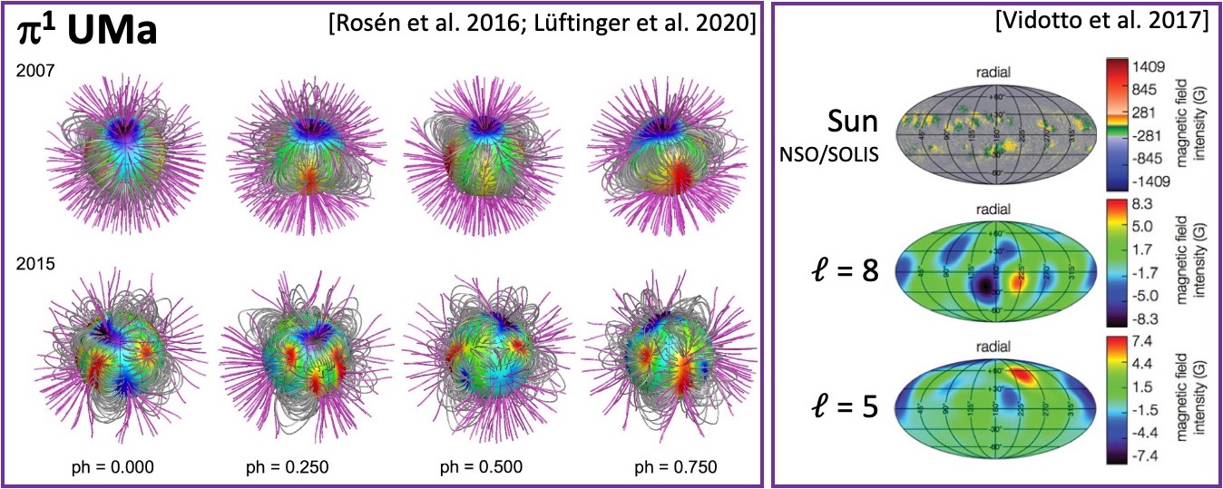
Figure 1: Left panel: ZDI stellar magnetograms of $\pi^{1}$ UMa obtained in 2007 and 2015 [from Rosén et al., 2016; Lüftinger et al., 2020]. Right panel: Comparison between solar $B_{r}$ magnetic field observations from NSO/SOLIS (top) with two low-degree PFSS reconstructions [from Vidotto, 2017].

A current limitation of the ZDI technique is illustrated in the right panel of Figure 1 [adapted from Vidotto, 2017]. The top row shows the vector magnetic field components obtained via NSO/SOLIS [Pevtsov, 2010; Bertello et al., 2013] whereas the middle and bottom rows show low-degree spherical harmonic representations ($\ell=8$ and $\ell=5$). In addition to lacking the overall spatial resolution required to resolve the strong-field active region flux systems observed on the Sun, the maximum field strengths are significantly underestimated (by roughly 2 orders of magnitude). In the young solar analog $\kappa^{1}$ Cet, ZDI synoptic magnetograms have maximum surface field strengths that are on the order of $\sim$20 G. However, measurements of unsigned magnetic flux from Zeeman broadening of the unpolarized Stokes I spectra suggest that $\kappa^{1}$ Cet has a disk-averaged, magnetic field magnitude of $\langle\,fB\,\rangle\sim 500$ G [e.g. Saar & Baliunas, 1992; Kochukhov et al., 2020]. This is the result of an unresolved magnetic flux in Stokes V (circularly polarized) observations due to an effective “cancellation” of the oppositely signed magnetic flux of starspots within pixel resolution via suppression of the Zeeman effect in dark regions [Kochukhov, 2016]. Thus, up to 90–95% of the magnetic flux is concentrated in small magnetic structures represented by stellar active regions/starspots that remain unresolved with current ZDI techniques [e.g. Reiners & Basri, 2009; See et al., 2019; Kochukhov, 2016; Kochukhov et al., 2020].

In general, the energy of solar/stellar flares ($E_{\rm flare}$) will be proportional to the free magnetic energy ($E_{M}$) stored in energized coronal magnetic field structures and thus can be written as $E_{\rm flare}\approx f_{c}E_{\rm M}=f_{c}\left(8\pi\right)^{-1}\left(B_{AR}\right)^{2}\left(A_{AR}\right)^{3/2}$ [Shibata et al., 2013; Maehara et al., 2015] where $f_{c}$ is a coefficient ($\leq 1$) describing the energy partition [Emslie et al., 2012]. To obtain the stellar flare/CME energies corresponding to so-called stellar “superflares” ($10^{\,\gtrsim 34}$ erg) in numerical MHD models, one must construct sufficiently strong magnetic fields over a large enough area.

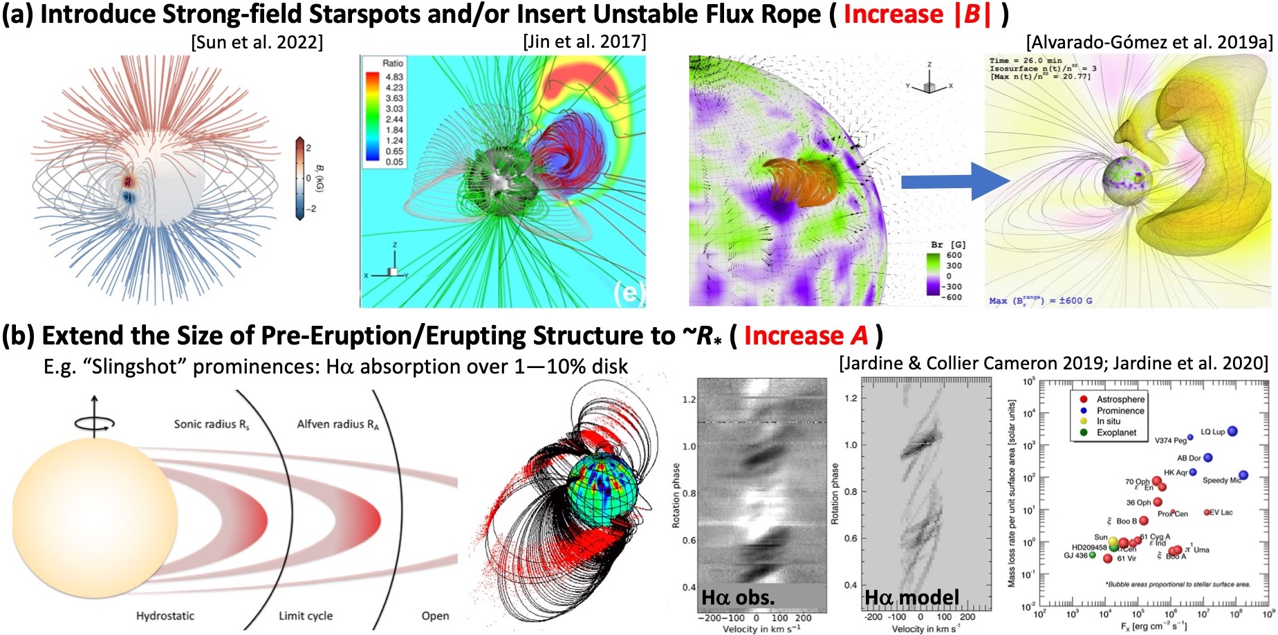
Figure 2: Two approaches to compensate for unresolved starspots/active region flux in order to obtain stellar superflare/CME energies of 10${}^{\,\gtrsim 34}$ erg consistent with observations. (a) Increasing the effective magnetic field strength of the CME source region through the addition of strong-field starspot active regions [Sun et al., 2022], the insertion of a highly energized, unstable flux rope [Jin et al., 2017], or some combination of the two [Alvarado-Gómez et al., 2019a]. (b) Increasing the effective area (size) of the CME source region through modeling large-scale, pre-eruption structures such as “slingshot prominences” which may regularly span the entire disk [Jardine & Collier Cameron, 2019; Jardine et al., 2020].

How do we deal with unresolved stellar active region flux? Figure 2 summarizes two (complementary) approaches for increasing $E_{M}$. The first approach is shown in Figure 2a, which illustrates examples of modeling large $|B|$ via the introduction of strong-field star spots [Sun et al., 2022], inserting an unstable magnetic flux rope [Jin et al., 2017], and what is effectively a combination of the two [Alvarado-Gómez et al., 2019a]. To constrain the field magnitude $B$, one can estimate the starspot/active region areas (filling-factor $f$ in the $\langle fB\rangle$ measurement), via transit observations where large starspot/active regions are usually identified as rotationally-modulated “dips” from dark regions on the stellar disk [Namekata et al., 2019]. Again, in the example of $\kappa{{}^{1}}$ Cet, Rucinski et al. [2004] and Walker et al. [2007] determined the light curve variations were consistent with two large starspots in 2003 (with areas of 1.4% and 3.6% of the stellar disk), three main starspots in 2004 (with areas of 1.9%, 5.3%, and 9% of the disk), and two spots in 2005 (2.2% and 2.9% of the stellar disk). These are at least a factor of 10 larger than the largest observed solar active region complexes [Hoge, 1947]. Future stellar observations could provide valuable information about smaller starspots/bipolar structures in optical and Far UV bands during their transit, as in the Sun-as-a-star study of Toriumi et al. [2020].

The second approach is shown in Figure 2b which presents a simple model for a pre-eruption, (potentially unstable) “slingshot prominence” structure that was estimated to cover a significant fraction of the stellar surface, i.e. large $A$, in order to explain observed H$\alpha$ absorption features [Jardine & Collier Cameron, 2019; Jardine et al., 2020]. The Figure 2b strategy of utilizing the largest possible source region area was employed by Lynch et al. [2019] to energize and erupt a 360^∘-wide streamer blowout CME. Figure 3 shows an overview of the Lynch et al. [2019] MHD simulation of a Carrington-scale eruptive flare and CME modeled with the ZDI synoptic magnetogram calculated by Rosén et al. [2016] for $\kappa{{}^{1}}$ Cet in August of 2012. Figure 3a,b show the stellar $B_{r}$ distribution and the global-scale, pre-eruption prominence-like field structure while Figure 3c shows a series of snapshots of the eruption in the ecliptic plane.

• Future modeling of stellar flare/CMEs will likely require one or both strategies to address the observational uncertainties in global and local magnetic field configurations of the flaring/CME source regions and should explore the eruption parameter space and resulting energy partition.

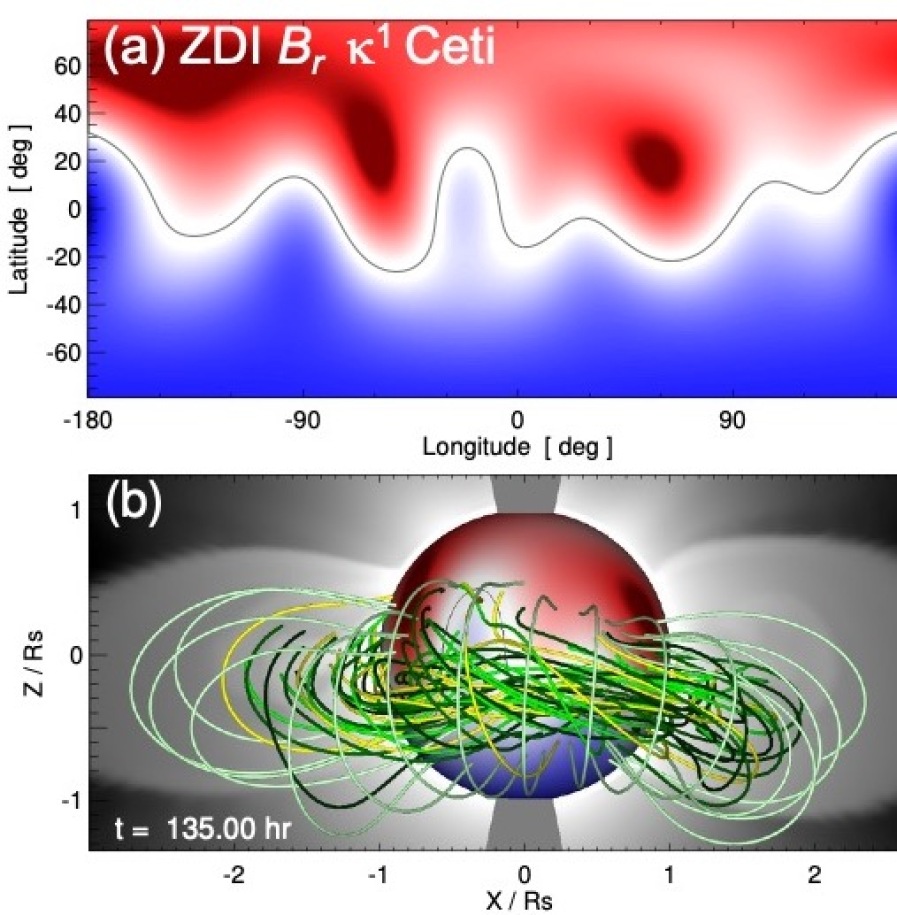
Figure 3: Overview of the Lynch et al. [2019] simulation of a Carrington-scale, X58 superflare and CME from the young solar analog $\kappa{{}^{1}}$ Cet. (a) ZDI magnetogram. (b) Energized, pre-eruption field structure. (c) CME evolution through 30$R_{\odot}$.

2.2 Measurements of Stellar Winds and Stellar CMEs (and their Limitations)

A fundamental difficulty with stellar wind research is that it is extremely hard to detect any component of coronal stellar winds, whether quiescent wind or transient CMEs. The most successful technique for studying stellar winds so far is by detecting hydrogen Lyman-$\alpha$ absorption from interaction regions between the winds and the surrounding interstellar medium, i.e. astrospheric absorption [Linsky & Wood, 1996; Wood et al., 2005]. However, even this technique has so far led to only 22 wind detections/measurements, and 7 useful upper limits [Wood et al., 2021]. Furthermore, this diagnostic is measuring the average wind ram pressure over long timescales, typically years to decades depending on the size of the astrosphere. Thus, it is unknown whether the observed stellar winds are dominated by quiescent wind or CMEs.

Candidate stellar CME detections are typically via observations not commonly used in solar CME research, meaning that it is not entirely certain the same phenomenon is being seen. That being said, significant progress has been made in the characterization and interpretation of stellar CME signatures by utilizing the results of multi-wavelength Sun-as-a-star analyses of large CME events [e.g.  Leitzinger et al., 2022; Namekata et al., 2022a, b; Xu et al., 2022].

A number of stellar CME claims originate from detection of blueshifted H$\alpha$ emission or absorption after stellar flares [Leitzinger et al., 2020; Muheki et al., 2020; Odert et al., 2020; Namekata et al., 2022b]. On the Sun, such observations would be called signatures of prominence/filament eruptions. While there are certainly cases where prominence material ends up incorporated into a CME that escapes the Sun [e.g. Wood et al., 2017; Lepri et al., 2014; Lepri & Rivera, 2021], this is not always the case, so an H$\alpha$ signature by itself would not necessarily be considered a CME detection. Blueshifted coronal lines observed after stellar flares have also been observed [Argiroffi et al., 2019; Namekata et al., 2022b].

One solar CME detection technique that does have potential applicability to how stars are observed is coronal dimming, demonstrated using full-disk SDO/EVE observations of low temperature coronal lines like Fe IX $\lambda$171 ($\log_{10}T/K\sim 5.8$) [Mason et al. 2016; see also Harra et al. 2016]. There are post-flare coronal dimmings that have been observed on stars, which have been interpreted as possible CMEs [Veronig et al., 2021; Loyd et al., 2022]. However, there is not a one-to-one correspondence between dimmings and the loss of coronal material via eruption, e.g. confined eruptions can also show dimming profiles at coronal temperatures [Alvarado-Gómez et al., 2019a].

Type II radio bursts are another promising stellar CME detection technique analogous to how CMEs (specifically, CME-driven shocks) are observed on the Sun. Such observations would have the added benefit of indicating the CME speed through the rate of change in radio frequency [Reiner et al., 2007; Liu et al., 2013]. Unfortunately, attempts to detect Type II bursts from frequently flaring M dwarfs, have so far proved unsuccessful [Crosley & Osten, 2018a, b; Villadsen & Hallinan, 2019]. While the solar CME–Type II association rate is only 4% overall [Bilenko, 2018], it is much higher for the most energetic CME events. The stellar Type II nondetections call into question the existence of fast, massive CMEs that are assumed to accompany the extremely energetic flares from M dwarf stars. The density jump of the CME-driven shock in the Lynch et al. [2019] simulation “predicted” electron plasma frequencies below the ionospheric cutoff of $\lesssim$20 MHz and the suppression/slow-down of stellar CMEs combined with the higher Alfvén speed profiles for active stars will result in a similar outcome [Alvarado-Gómez et al., 2020b], making ground-based detection extremely difficult.

• Simultaneous multi-wavelength observations of potential stellar CME signatures (e.g. H$\alpha$, X-ray and UV dimmings, radio bursts) are expected to makes significant progress toward resolving at least some of the current observational ambiguities, especially with complementary Sun-as-a-star analyses of solar flares/filament eruptions/CMEs in H$\alpha$ and EUV wavelengths. Both idealized and “data-constrained” modeling of stellar winds and flares/CMEs should aim to generate synthetic observables at different wavelengths for observational guidance and to quantify detectability thresholds.

2.3 Do Solar–Stellar “Scaling Laws” Break Down?

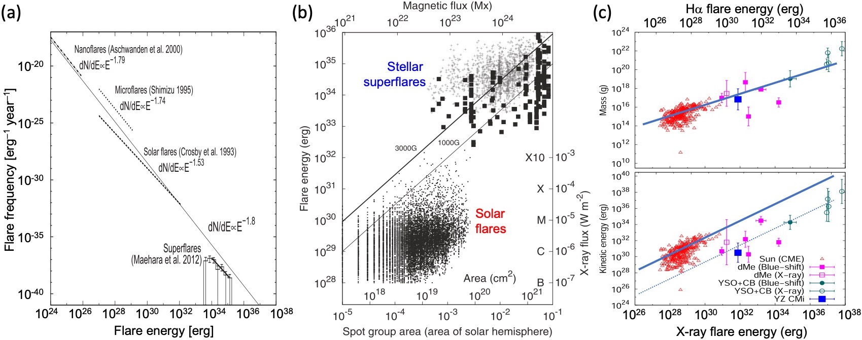
Figure 4: Solar–stellar scaling laws. (a) Flare frequency vs. energy [Shibata et al., 2013]. (b) Flare energy vs. active region area [Maehara et al., 2015]. (c) CME mass and kinetic energy vs. X-ray and H$\alpha$ flare energy [Maehara et al., 2021].

For the Sun, a strong correlation is found between flare strength as quantified by X-ray luminosity and CME mass [e.g. Aarnio et al., 2011]. Given that we have very limited observational knowledge about the nature of CMEs emanating from other stars, it is natural to apply solar flare/CME relations to active stars that flare more frequently and energetically, in order to estimate what CMEs might contribute to the stellar winds of these stars [Moschou et al., 2019].

Figure 4 demonstrates a number of solar–stellar scaling laws. Figure 4a, adapted from Shibata et al. [2013], plots the power-law distributions obtained for flare occurrence frequency as a function of energy, spanning $\sim$10 orders of magnitude from nanoflares [Aschwanden et al., 2000], to microflares [Shimizu, 1995], “standard” solar flares [Crosby et al., 1993], and stellar superflares [Maehara et al., 2012]. The power-law $dN/dE\propto E^{-1.8}$ is shown as the thin solid line and appears reasonably consistent with the observed occurrence frequencies over the entire flare energy range. Figure 4b, adapted from Maehara et al. [2015], shows flare energy vs. solar/stellar spot area (and associated unsigned magnetic flux). The grouping of solar flares and stellar superflares are labeled accordingly and the thick (thin) solid line corresponds to the $E_{\rm flare}$ expression of Section 2.1 as a function of $A_{AR}$ assuming $f_{c}=0.10$ and constant $B_{AR}$ values of 1 kG (3 kG), respectively.

Figure 4c, adapted from Maehara et al. [2021], shows the CME mass ($M_{\rm cme}$; upper panel) and kinetic energy ($E_{K}$; lower panel) estimates vs. flare (X-ray) energy (or equivalently, the flare H$\alpha$ energy as a simple rescaling of the X-ray energy). The set of solar flare–CME points [from Yashiro & Gopalswamy, 2009] are shown as red triangles, candidate stellar eruptive flare/CME detections as the blue, magenta, and teal points, along with the power-law fits obtained by Drake et al. [2013]: $M_{\rm cme}\propto E_{\rm X-ray}^{0.59\pm 0.02}$ and $E_{K}\propto E_{\rm X-ray}^{1.05\pm 0.03}$ (blue lines). It is interesting to note that the $M_{\rm cme}$ scaling appears consistent between the solar and stellar cases whereas $E_{K}$ estimated for the stellar events are comfortably below the extrapolated solar scaling law by 2–3 orders of magnitude. This may be a result of simply underestimating the stellar CME values because the prominence material (as the source of H$\alpha$ absorption/emission) is merely a subset of the larger CME erupting structure, or that these potential stellar CME detections are representative of magnetic environments that impede traditional “solar-like” CME eruptions and their evolution through extended stellar coronae [e.g. as in Alvarado-Gómez et al., 2018].

Merely extrapolating to stellar regimes from solar data for truly active stars invariably leads to conclusions that such stars should have winds hundreds or thousands of times stronger than the solar wind simply due to CMEs alone [e.g. Drake et al. 2013; Odert et al. 2017; Figure 4c]. Such conclusions not only conflict with the Type II radio burst nondetections, but they also conflict with a failure to detect such strong winds using the aforementioned astrospheric Lyman-$\alpha$ absorption technique [Wood et al., 2021]. For example, the astrospheric measurements suggest mass-loss rates of only 1 and 30 times the solar mass-loss rate for the notorious M dwarf flare stars EV Lac and YZ CMi, respectively. Clearly, the strong connection between flares and fast, massive CMEs on the Sun cannot extend to flare stars like EV Lac and YZ CMi. For such stars, CMEs must be far less common or far less massive than one might expect, given the frequent flaring.

The Sun itself may provide clues for what is happening on active flare stars, as there are many cases of strong flares with no associated CME. A well-studied example is the series of X-class flares from active region NOAA 12192, which was highly flare-productive, particularly in 2014 October. However, almost none of the flares from AR 12192 had associated CMEs [Sun et al., 2015; Thalmann et al., 2015]. On the Sun, this is unusual, but on active stars perhaps this is the norm. Strong magnetic fields overlying an active region can inhibit CME eruption. Numerical simulations of CMEs on active stars made in recent years include models of such confined eruptions [Alvarado-Gómez et al., 2018; Alvarado-Gómez et al., 2019a, b, 2020b], and Sun et al. [2022] performed a theoretical study of the susceptibility of stellar active regions to the torus instability for CME initiation [Kliem & Török, 2006], which explores why active stars may be less prone to CMEs than generally supposed.

• We strongly encourage research designed to explore the physical conditions leading to both successful and “confined” eruptions in order to understand the regimes where the semi-empirical solar–stellar scaling laws appear to work and those where they do not.

3 Stellar Space Weather Impacts on Exoplanetary Atmospheres

One important application of stellar wind measurements is to better understand the environment of exoplanets around cool stars. The M dwarfs are of particular interest due in part to the abundance of such stars in the galaxy. Also, the habitable zones of the intrinsically faint M dwarfs are much closer to the stars than for earlier type stars like the Sun, so planets in such locations will potentially be exposed to much higher particle fluxes from stellar winds. Assessments of the potential impact of this wind exposure on planets in M dwarf systems have been underway for some time [e.g. Vidotto et al. 2013; Garraffo et al. 2016; Dong et al. 2017; Alvarado-Gómez et al. 2019b, 2020a]. Figure 5 presents three recent examples of star-to-planet modeling to explore the impact of steady-state stellar winds on exoplanets in the TRAPPIST-1 [upper left; Garraffo et al., 2017], TOI-700 [lower left; Dong et al., 2020], and Proxima Centari [right; Alvarado-Gómez et al., 2020a] systems.

Whether M dwarf habitable zone planets are truly habitable is in part tied to the question of whether intense exposure of such stars to stellar flares, CMEs, and energetic particles would make habitability impossible [e.g. Khodachenko et al. 2007; Yamashiki et al. 2019; Hu et al. 2022]. If fast, massive CMEs from frequently flaring M dwarfs are less common than generally thought, perhaps CME exposure is not as big a factor for habitability as often supposed. Furthermore, in the solar case, the most damaging energetic particles originate from CME shocks rather than flares, if fast CMEs are less common than generally thought, perhaps energetic particle fluxes are also lower [Fraschetti et al., 2019]. Exoplanets in M dwarf habitable zones will certainly be exposed to high X-ray fluxes, both from quiescent coronal emission and flares, but it remains an open question whether solar models of coronal heating and wind acceleration can be applied to M dwarfs and how significant stellar CMEs and energetic particle fluxes are to long-term atmospheric evolution, and ultimately, to exoplanet habitability.

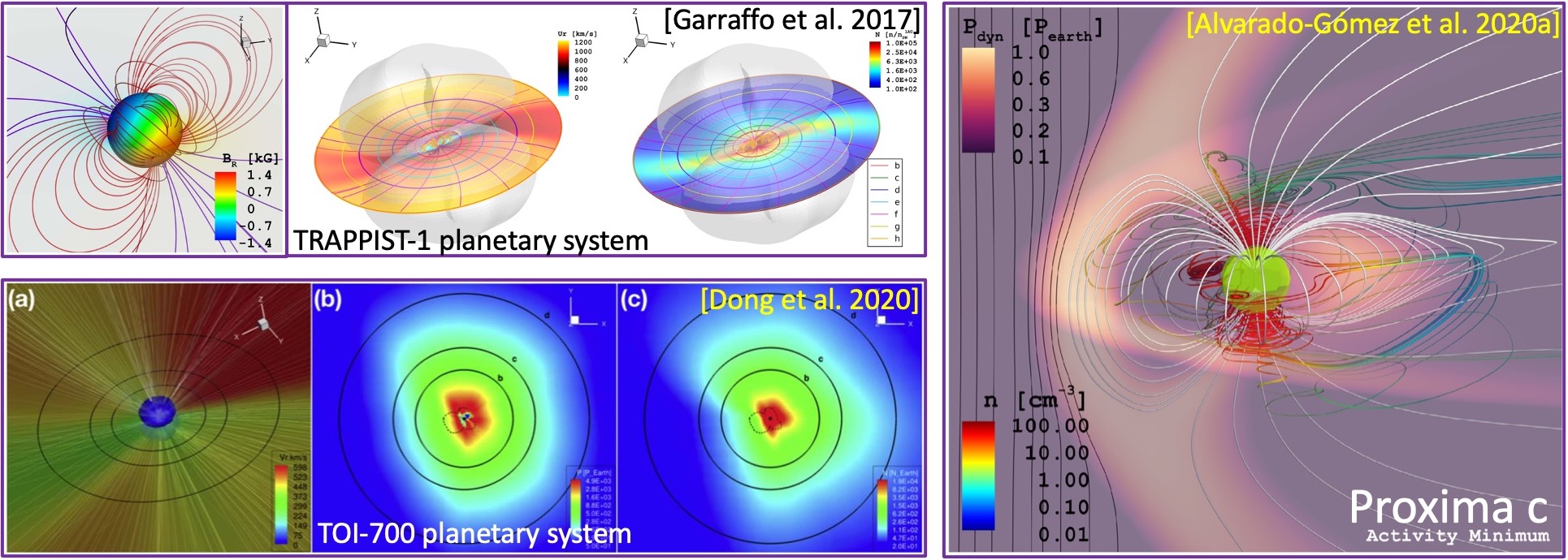
Figure 5: Modeling stellar winds and star–planet interactions: TRAPPIST-1 system [upper left; Garraffo et al., 2017], TOI-700 system [lower left; Dong et al., 2020], and for Proxima c [right; Alvarado-Gómez et al., 2020a].

• Future application of heliophysics modeling tools to star-to-planet systems should aspire to be as “data-constrained” as possible (to limit the wind and flare/CME model parameter spaces) and include forward modeling of synthetic observable quantities, i.e. spectral signatures of atmospheric composition, chemistry and evolution/loss, auroral emission, etc.

4 Recommendations for Future Research Directions

• Theoretical and numerical studies of CME initiation and low coronal evolution, including confinement of “failed” eruptions. Existing measurements of active stars suggest that most(?) of these stellar flares may represent confined eruptions without an accompanying “solar-like” CME. Future research should characterize solar active region sources of confined eruptions, quantify the confined/eruptive thresholds, and investigate the implications for stellar magnetic field configurations that inhibit or facilitate CMEs from stellar superflares.

• Systematic analyses of Sun-as-a-star observations to develop and improve stellar CME detection techniques and alternatives, including but not limited to: disk-integrated brightening and dimming in EUV and X-ray spectral lines/wavelength ranges; quantitative forward modeling of flare, CME, and CME-driven shock radio emission; data analysis and forward modeling of eruption-induced Doppler shifts in H$\alpha$ and UV lines.

• Improvements in data-inspired and data-constrained MHD modeling of solar CMEs and their application to stellar systems. Develop holistic, full star-to-planet system modeling (or sequence of models) to characterize the range of exoplanetary space weather star–planet interactions and their impact on exoplanetary atmospheres over evolutionary timescales.

• Encourage comprehensive solar–stellar research collaborations and conferences through new interdisciplinary and multi-agency/division funding mechanisms. The multidisciplinary nature of this type of solar–stellar research is likely to require coordinated “Centers of Excellence” organizational/institutional support somewhat analogous to the NASA Astrobiology Institutes, the Heliophysics DRIVE centers, or the joint NSF–NASA funding structures that have supported multi-institution Space Weather research networks. Smaller focused efforts should also be supported through, e.g., future NASA LWS FST topics, expanded XRP funding, and other opportunities with solar/stellar overlap such as NSF AAG/AGS programs.

References

- Aarnio et al. [2011] Aarnio, A. N., et al. 2011, Sol. Phys., 268, 195
- Airapetian et al. [2020] Airapetian, V. S., et al. 2020, \ijasb, 19, 136
- Alvarado-Gómez et al. [2018] Alvarado-Gómez, J. D., et al. 2018, ApJ, 862, 93
- Alvarado-Gómez et al. [2020a] Alvarado-Gómez, J. D., et al. 2020a, ApJ, 902, L9
- Alvarado-Gómez et al. [2019a] Alvarado-Gómez, J. D., et al. 2019a, ApJ, 884, L13
- Alvarado-Gómez et al. [2019b] Alvarado-Gómez, J. D., et al. 2019b, ApJ, 875, L12
- Alvarado-Gómez et al. [2020b] Alvarado-Gómez, J. D., et al. 2020b, ApJ, 895, 47
- Andrews [2003] Andrews, M. D. 2003, Sol. Phys., 218, 261
- Argiroffi et al. [2019] Argiroffi, C., et al. 2019, \natas, 3, 742
- Aschwanden et al. [2000] Aschwanden, M. J., et al. 2000, ApJ, 535, 1047
- Bertello et al. [2013] Bertello, L., et al. 2013, AAS/SPD, 44, 100.135
- Bilenko [2018] Bilenko, I. A. 2018, \geae, 58, 989
- Bourrier et al. [2016] Bourrier, V., et al. 2016, A&A, 591, A121
- Brennan [2022] Brennan, P. 2022, Cosmic Milestone: NASA Confirms 5,000 Exoplanets. Accessed: 2022-04-05
- Carmichael [1964] Carmichael, H. 1964, NASA SP, 50, 451
- Cherenkov et al. [2017] Cherenkov, A., et al. 2017, ApJ, 846, 31
- Cohen et al. [2011] Cohen, O., et al. 2011, ApJ, 738, 166
- Crosby et al. [1993] Crosby, N. B., et al. 1993, Sol. Phys., 143, 275
- Crosley & Osten [2018a] Crosley, M. K., & Osten, R. A. 2018a, ApJ, 856, 39
- Crosley & Osten [2018b] Crosley, M. K., & Osten, R. A. 2018b, ApJ, 862, 113
- do Nascimento et al. [2016] do Nascimento, Jr., J.-D., et al. 2016, ApJ, 820, L15
- Donati et al. [1997] Donati, J.-F., et al. 1997, MNRAS, 291, 658
- Dong et al. [2020] Dong, C., et al. 2020, ApJ, 896, L24
- Dong et al. [2017] Dong, C., et al. 2017, ApJ, 837, L26
- Drake et al. [2013] Drake, J. J., et al. 2013, ApJ, 764, 170
- Ekenbäck et al. [2010] Ekenbäck, A., et al. 2010, ApJ, 709, 670
- Emslie et al. [2012] Emslie, A. G., et al. 2012, ApJ, 759, 71
- Fletcher et al. [2011] Fletcher, L., et al. 2011, Space Sci. Rev., 159, 19
- Forbes [2000] Forbes, T. G. 2000, J. Geophys. Res., 105, 23153
- Fraschetti et al. [2019] Fraschetti, F., et al. 2019, ApJ, 874, 21
- Garraffo et al. [2016] Garraffo, C., et al. 2016, ApJ, 833, L4
- Garraffo et al. [2017] Garraffo, C., et al. 2017, ApJ, 843, L33
- Gopalswamy et al. [2005] Gopalswamy, N., et al. 2005, J. Geophys. Res., 110, A12S07
- Green et al. [2018] Green, L. M., et al. 2018, Space Sci. Rev., 214, 46
- Harra et al. [2016] Harra, L. K., et al. 2016, Sol. Phys., 291, 1761
- Hazra et al. [2022] Hazra, G., et al. 2022, MNRAS, 509, 5858
- Hirayama [1974] Hirayama, T. 1974, Sol. Phys., 34, 323
- Hoge [1947] Hoge, E. R. 1947, PASP, 59, 109
- Hu et al. [2022] Hu, J., et al. 2022, \sciadv, 8, eabi9743
- Jakosky et al. [2018] Jakosky, B. M., et al. 2018, Icarus, 315, 146
- Janvier et al. [2015] Janvier, M., et al. 2015, Sol. Phys., 290, 3425
- Jardine & Collier Cameron [2019] Jardine, M., & Collier Cameron, A. 2019, MNRAS, 482, 2853
- Jardine et al. [2020] Jardine, M., et al. 2020, MNRAS, 491, 4076
- Jin et al. [2017] Jin, M., et al. 2017, ApJ, 834, 173
- Kazachenko et al. [2012] Kazachenko, M. D., et al. 2012, Sol. Phys., 277, 165
- Khodachenko et al. [2007] Khodachenko, M. L., et al. 2007, Astrobiology, 7, 167
- Kislyakova et al. [2014] Kislyakova, K. G., et al. 2014, Science, 346, 981
- Kliem & Török [2006] Kliem, B., & Török, T. 2006, Phys. Rev. Lett., 96, 255002
- Klimchuk [2001] Klimchuk, J. A. 2001, AGU GMS, 125
- Kochukhov [2016] Kochukhov, O. 2016 in LNP, Vol. 914, 177
- Kochukhov et al. [2020] Kochukhov, O., et al. 2020, A&A, 635, A142
- Kopp & Pneuman [1976] Kopp, R. A., & Pneuman, G. W. 1976, Sol. Phys., 50, 85
- Lammer et al. [2007] Lammer, H., et al. 2007, Astrobiology, 7, 185
- Lecavelier Des Etangs et al. [2010] Lecavelier Des Etangs, A., et al. 2010, A&A, 514, A72
- Leitzinger et al. [2022] Leitzinger, M., et al. 2022, MNRAS, 513, 6058
- Leitzinger et al. [2020] Leitzinger, M., et al. 2020, MNRAS, 493, 4570
- Lepri & Rivera [2021] Lepri, S. T., & Rivera, Y. J. 2021, ApJ, 912, 51
- Lepri et al. [2014] Lepri, S. T., et al. 2014 in IAUS, Vol. 300, 289–296
- Linsky & Wood [1996] Linsky, J. L., & Wood, B. E. 1996, ApJ, 463, 254
- Liu et al. [2013] Liu, Y. D., et al. 2013, ApJ, 769, 45
- Loyd et al. [2022] Loyd, R. O. P., et al. 2022, \arxiv, 2207.05115
- Lüftinger et al. [2020] Lüftinger, T., et al. 2020 in Origins: From the Protosun to the First Steps of Life, Vol. 345, 181–184
- Lüftinger et al. [2010a] Lüftinger, T., et al. 2010a, A&A, 509, A71
- Lüftinger et al. [2015] Lüftinger, T., et al. 2015 in ASSL, Vol. 411, 37
- Lüftinger et al. [2010b] Lüftinger, T., et al. 2010b, A&A, 509, A43
- Lynch et al. [2019] Lynch, B. J., et al. 2019, ApJ, 880, 97
- Lynch et al. [2021] Lynch, B. J., et al. 2021, ApJ, 914, 39
- Maehara et al. [2015] Maehara, H., et al. 2015, \eps, 67, 59
- Maehara et al. [2012] Maehara, H., et al. 2012, Nature, 485, 478
- Maehara et al. [2021] Maehara, H., et al. 2021, PASJ, 73, 44
- Mason et al. [2016] Mason, J. P., et al. 2016, ApJ, 830, 20
- Moschou et al. [2019] Moschou, S.-P., et al. 2019, ApJ, 877, 105
- Muheki et al. [2020] Muheki, P., et al. 2020, A&A, 637, A13
- Namekata et al. [2022a] Namekata, K., et al. 2022a, ApJ, 933, 209
- Namekata et al. [2019] Namekata, K., et al. 2019, ApJ, 871, 187
- Namekata et al. [2022b] Namekata, K., et al. 2022b, \natas, 6, 241
- Odert et al. [2020] Odert, P., et al. 2020, MNRAS, 494, 3766
- Odert et al. [2017] Odert, P., et al. 2017, MNRAS, 472, 876
- Pevtsov [2010] Pevtsov, A. 2010 in 38th COSPAR Assembly, Vol. 38, 2
- Piskunov & Kochukhov [2002] Piskunov, N., & Kochukhov, O. 2002, A&A, 381, 736
- Reiner et al. [2007] Reiner, M. J., et al. 2007, ApJ, 663, 1369
- Reiners & Basri [2009] Reiners, A., & Basri, G. 2009, A&A, 496, 787
- Rosén et al. [2016] Rosén, L., et al. 2016, A&A, 593, A35
- Rucinski et al. [2004] Rucinski, S. M., et al. 2004, PASP, 116, 1093
- Saar & Baliunas [1992] Saar, S. H., & Baliunas, S. L. 1992 in \aspc, ed. K. L. Harvey, Vol. 27, 197–202
- Schneiter et al. [2016] Schneiter, E. M., et al. 2016, MNRAS, 457, 1666
- See et al. [2019] See, V., et al. 2019, ApJ, 876, 118
- Shibata & Magara [2011] Shibata, K., & Magara, T. 2011, \lrsp, 8, 6
- Shibata et al. [2013] Shibata, K., et al. 2013, PASJ, 65, 49
- Shimizu [1995] Shimizu, T. 1995, PASJ, 47, 251
- Sturrock [1966] Sturrock, P. A. 1966, Nature, 211, 695
- Sun et al. [2022] Sun, X., et al. 2022, MNRAS, 509, 5075
- Sun et al. [2015] Sun, X., et al. 2015, ApJ, 804, L28
- Thalmann et al. [2015] Thalmann, J. K., et al. 2015, ApJ, 801, L23
- Toriumi et al. [2020] Toriumi, S., et al. 2020, ApJ, 902, 36
- Török et al. [2018] Török, T., et al. 2018, ApJ, 856, 75
- Veronig et al. [2021] Veronig, A. M., et al. 2021, \natas, 5, 697
- Vidal-Madjar et al. [2003] Vidal-Madjar, A., et al. 2003, Nature, 422, 143
- Vidotto [2017] Vidotto, A. A. 2017 in IAUS, Vol. 328, 237–239
- Vidotto [2021] Vidotto, A. A. 2021, \lrsp, 18, 3
- Vidotto et al. [2013] Vidotto, A. A., et al. 2013, A&A, 557, A67
- Vidotto et al. [2011] Vidotto, A. A., et al. 2011, MNRAS, 412, 351
- Villadsen & Hallinan [2019] Villadsen, J., & Hallinan, G. 2019, ApJ, 871, 214
- Walker et al. [2007] Walker, G. A. H., et al. 2007, ApJ, 659, 1611
- Wood et al. [2005] Wood, B. E., et al. 2005, ApJ, 628, L143
- Wood et al. [2017] Wood, B. E., et al. 2017, ApJS, 229, 29
- Wood et al. [2021] Wood, B. E., et al. 2021, ApJ, 915, 37
- Xu et al. [2022] Xu, Y., et al. 2022, ApJ, 931, 76
- Yamashiki et al. [2019] Yamashiki, Y. A., et al. 2019, ApJ, 881, 114
- Yashiro & Gopalswamy [2009] Yashiro, S., & Gopalswamy, N. 2009 in Universal Heliophysical Processes, Vol. 257, 233–243
- Zhang et al. [2021] Zhang, J., et al. 2021, \peps, 8, 56