Foundation Transformers

Abstract

A big convergence of model architectures across language, vision, speech, and multimodal is emerging. However, under the same name “Transformers”, the above areas use different implementations for better performance, e.g., Post-LayerNorm for BERT, and Pre-LayerNorm for GPT and vision Transformers. We call for the development of Foundation Transformer for true general-purpose modeling, which serves as a go-to architecture for various tasks and modalities with guaranteed training stability. In this work, we introduce a Transformer variant, named Magneto, to fulfill the goal. Specifically, we propose Sub-LayerNorm for good expressivity, and the initialization strategy theoretically derived from DeepNet (Wang et al., 2022a) for stable scaling up. Extensive experiments demonstrate its superior performance and better stability than the de facto Transformer variants designed for various applications, including language modeling (i.e., BERT, and GPT), machine translation, vision pretraining (i.e., BEiT), speech recognition, and multimodal pretraining (i.e., BEiT-3).

Models			Previous	This work
Vision	Encoder	ViT/BEiT	Pre-LN	Sub-LN
Language	Encoder	BERT	Post-LN
	Decoder	GPT	Pre-LN
	Encoder-Decoder	NMT/BART	Post-LN
Speech	Encoder	T-T	Pre-LN
Multimodal	Encoder	BEiT-3	Pre-LN

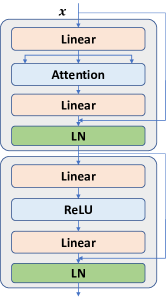
(a) Post-LN

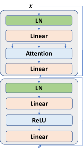
(b) Pre-LN

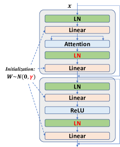
(c) Sub-LN

Figure 1: Top: the architectures of SOTA models across language, vision, speech, and multimodal. Bottom: the proposed Foundation Transformer uses Sub-LN and theoretically derived initialization.

1 Introduction

Recent years have witnessed a big convergence of model architectures across language, vision, speech, and multimodal. Specifically, starting from the natural language processing, Transformers (Vaswani et al., 2017) have become the de facto standard for various areas, including computer vision (Dosovitskiy et al., 2021), speech (Zhang et al., 2020b), and multimodal (Kim et al., 2021; Wang et al., 2022b). Transformers fully leverage the parallelism advantage of GPU hardware and large-scale data. It is appealing that we can use the same network architecture for a broad range of applications. So the pretrained models can be seamlessly reused with the shared implementation and hardware optimization. Moreover, general-purpose modeling is important to multimodal models, as different modalities can be jointly encoded and fused by one model.

However, despite using the same name “Transformers”, there are significant differences in the implementation of the architectures for different tasks. Figure 1 summarizes the architectures for state-of-the-art models that are widely used in various communities. For instance, some models (e.g., GPT, and ViT) adopt Pre-LayerNorm (Pre-LN) Transformers, while others use Post-LayerNorm (Post-LN) variants (e.g., BERT, and machine translation) for better performance. Rather than directly using the same architecture, we need to compare two Transformer variants on the specific tasks or modalities to determine the backbone, which is ineffective for model development. More importantly, considering multimodal models, the optimal Transformer variants are usually different for input modalities. For the example of BEiT-3 (Wang et al., 2022b) vision-language pretraining, using Post-LN is sub-optimal for vision encoding while Pre-LN is sub-optimal for the language part. The true convergence of multimodal pretraining requires a unified architecture that performs well across tasks and modalities. In addition, a pain point of Transformer architectures is training stability, especially for large-scale models. We usually need significant efforts to tune hyperparameters or babysit training processes.

As a result, we call for developing Foundation Transformers for true general-purpose modeling. First, the desired modeling should be able to serve as a go-to architecture for various tasks and modalities, so that we can use the same backbone without trial and error. The general-purpose design principle also greatly supports the development of multimodal foundation models, as we can use one unified Transformer for various modalities without performance degradation. Second, the architectures should provide guaranteed training stability. The favored property can significantly mitigate the difficulty of large-scale pretraining of foundation models.

In this work, we introduce Magneto as an implementation of Foundation Transformers to fulfill the above goals. Specifically, we introduce Sub-LayerNorm (Sub-LN), which adds an extra LayerNorm to each sublayer (i.e., multi-head self-attention, and feed-forward network). Moreover, Magneto has a novel initialization method that has a theoretical guarantee to fundamentally improve the training stability. This allows the models to be scaled up without pain. We evaluate Magneto on extensive tasks and modalities, namely, masked language modeling (i.e., BERT), causal language modeling (i.e., GPT), machine translation, masked image modeling (i.e., BEiT), speech recognition, and vision-language pretraining (i.e., BEiT-3). Experimental results show that Magneto significantly outperforms de facto Transformer variants on the downstream tasks. In addition, Magneto is more stable in terms of optimization, which allows larger learning rates to improve results without training divergence.

2 TL;DR for Practitioners

⬇

def subln(x):

return x + fout(LN(fin(LN(x))))

def subln_init(w):

if w is ['ffn', 'v_proj', 'out_proj']:

nn.init.xavier_normal_(w, gain=$\gamma$)

elif w is ['q_proj', 'k_proj']:

nn.init.xavier_normal_(w, gain=1)

Architectures	Encoder	Decoder
	$\gamma$	$\gamma$
Encoder-only	$\sqrt{\log{2N}}$	-
(e.g., BERT, ViT)
Decoder-only	-	$\sqrt{\log{2M}}$
(e.g., GPT)
Encoder-decoder	$\sqrt{\frac{1}{3}\log{3M}\log{2N}}$	$\sqrt{\log{3M}}$
(e.g., NMT, BART)

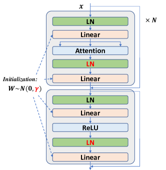
(a) Encoder or Decoder

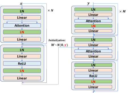
(b) Encoder-Decoder

Figure 2: Top left: pseudocode of Sub-LN. We take Xavier initialization (Glorot and Bengio, 2010) as an example, and it can be replaced with other standard initialization. Notice that $\gamma$ is a constant. Top right: parameters of Sub-LN for different architectures ($N$-layer encoder, $M$-layer decoder). Bottom: the layout of Sub-LN for different architectures.

Figure 1 illustrates the overview of the Magneto architecture. There are two key improvements in terms of modeling. First, compared to the Pre-LN variant, Sub-LN introduces another LayerNorm inside each sublayer (i.e., multi-head self-attention, and feed-forward network): one before the input projection, and the other before the output projection. Second, we use the initialization with the theoretical derivation from DeepNet (Wang et al., 2022a), which fundamentally improves the training stability, allowing the model to be scaled up to massive sizes without pain.

As shown in Figure 2, we present the implementation of Magneto. There are only lines of code changes on top of the vanilla Transformer architecture. Notably, following the derivation from DeepNet, the weights of query projection and key projection are not scaled during initialization. Besides, there is only one LayerNorm inside the cross-attention for the encoder-decoder architecture and we do not scale the initialized weights of cross-attention.

3 Magneto: A Foundation Transformer

3.1 Architecture: Sub-LayerNorm

Vanilla Transformers are based on either Pre-LayerNorm (Pre-LN) structures or Post-LayerNorm (Post-LN). Different from them, Magneto is built on the Sub-LayerNorm (Sub-LN). It inherits the multihead attentions and the feed-forward network from Transformers and introduces two layer normalization modules inside each sublayer (except the cross-attention).

For the multihead attentions, the layer normalization modules are before the $qkv$ projection and the output projection, which can be formulated as:

$$Q,K,V =W^{Q}\text{LN}(x),W^{K}\text{LN}(x),W^{V}\text{LN}(x)$$ (1)

$$\text{MSA}(x) =x+W^{O}\text{LN}(\text{Attention}(Q,K,V))$$ (2)

where $W^{Q}$, $W^{K}$, $W^{V}$, and $W^{O}$ are the parameters of the multihead self-attention. Similarly, for the feed-forward network, the layer normalization modules are before the input projection and the output projection, which are written as:

$$\text{FC}_{1}(x) =W^{1}\text{LN}(x)$$ (3)

$$\text{FC}_{2}(x) =W^{2}\text{LN}(x)$$ (4)

$$\text{FFN}(x) =\text{FC}_{2}(\phi(\text{FC}_{1}(x)))$$ (5)

where $W^{1}$ and $W^{2}$ are parameters of the feed-forward layers, and $\phi$ is the non-linear activation function.

3.2 Initialization: Theoretical Derivation from DeepNet

We adopt the theoretical derivation from DeepNet (Wang et al., 2022a) to improve the training stability. DeepNet estimates the expected model update for Post-LN and introduces DeepNorm to bound the model update to a constant. Following DeepNet, we first estimate the expected model update of Sub-LN and then demonstrate how to bound the model update with a proper initialization.

Expected Model Update for Pre-LN

We start with the expected model update for Pre-LN. The forward propagation for an $N$-layer Pre-LN Transformer with $N$ attention sub-layers and $N$ feed-forward sub-layers can be formulated as:

$$F(x;\theta)=W^{vocab}x^{e}$$ (6)

$$x^{e}=\text{LN}(x+\sum_{l=1}^{L}G^{l}(x^{l-1},\theta_{el})),\quad x^{l}=G^{l}(x^{l-1},\theta_{el})\,\text{and}\,x^{0}=x$$ (7)

where $x^{l-1}$, $x^{l}$ denotes the input and output for the $l$-th sub-layer $G^{l}$. If $l$ is odd, $G^{l}$ refers to self-attention MSA; if $l$ is even, $G^{l}$ refers to FFN. $x^{e}$ is the output of the backbone. $\theta$ denotes the parameters of output projection $W^{vocab}$ and the backbone $\{\theta_{el}\}_{l=1}^{L}$. $W^{vocab}\in R^{V\times d}$, where $d$ is hidden dimension, $V$ is dictionary size. $L$ equals to $2N$ for simplicity. Without the loss of generality, we set the intermediate dimension of feed-forward layers equals to hidden dimension.

Following Wang et al. (2022a), the magnitude of attention output only depends on value and output projection: $\text{MSA}(X)\overset{\Theta}{=}W^{O}W^{V}\text{LN}(X)$. Similarly we have $\text{FFN}(x)=W^{2}\phi(W^{1}\text{LN}(X))$. Therefore, for vanilla Pre-LN, the forward computation of the $l$-th sub-layer can be formulated as:

$$x^{l}=x^{l-1}+W^{l,2}\phi(W^{l,1}\text{LN}(x^{l-1}))$$ (8)

We introduce two constants $v_{l},w_{l}$ to represent the scales of $W^{l,2},W^{l,1}$ respectively. For example, the $i$-th row, $j$-th column entry of $W^{l,2}$ satisfies that:

$$W_{ij}^{l,2}\backsim\mathcal{N}(0,\cfrac{v_{l}^{2}}{d})$$ (9)

We define the model update $\Delta F=||\gamma^{T}(F(x;\theta^{*})-F(x;\theta))||$, where $\gamma,F(x)\in$ $R^{V\times 1}$. $x$ and $F(x)$ denote the input and output of the model respectively. $\gamma$ is the label of $x$, which is a one-hot vector with a single entry as 1 and all the others as 0. With above analysis, we have the following theorem to characterize $\Delta F^{pre}$ for an $N$-layer, encoder-only Pre-LN Transformer under SGD update.

Theorem 3.1.

Given an $N$-layer Pre-LN Transformer $F(x,\mathbf{\theta})$, the $l$-th sub-layer is formulated as $x^{l}=x^{l-1}+W^{l,2}\phi(W^{l,1}\text{LN}(x^{l-1}))$. Under SGD update, $\Delta F^{pre}$ satisfies:

$$\Delta F^{pre}\leq\eta d(\cfrac{\sum_{l=1}^{L}v_{l}^{2}+w_{l}^{2}}{\sum_{n=1}^{L}v_{n}^{2}w_{n}^{2}}+\sum_{l=1}^{L}\sum_{k=2}^{L}\cfrac{v_{l}^{2}+w_{l}^{2}}{\sum_{n=1}^{L}v_{n}^{2}w_{n}^{2}}\,\cfrac{v_{k}^{2}w_{k}^{2}}{\sum_{n=1}^{k-1}v_{n}^{2}w_{n}^{2}}))$$ (10)

where $\eta$ is learning rate, $L$ equals to $2N$.

Based on Theorem 3.1, with $v_{l}=w_{l}=1$ (i.e., standard initialization) for vanilla Pre-LN, we have $\Delta F^{pre}=\mathcal{O}(\eta d\log L)$, which shows that the magnitude of the model update grows logarithmically as the depth increases. It is also verified by Liu et al. (2020). Wang et al. (2022a) proves that under SGD update, the model update of vanilla Post-LN $\Delta F^{post}$ is $\mathcal{O}(\sum_{l=1}^{L}v_{l}^{2}+w_{l}^{2})$. $\Delta F^{pre}$ is much smaller than $\Delta F^{post}$ with the same model depth $L$. It indicates that the loss landscape of vanilla Pre-LN is smoother than that of vanilla Post-LN, which leads to faster and more stable optimization.

Expected Model Update for Magneto

Based on the analysis on Pre-LN, we further estimate the expected model update of Sub-LN. With Sub-LN, the forward signal propagation of the $l$-th sub-layer can be formulated as:

$$x^{l}=x^{l-1}+W^{l,2}\text{LN}(\phi(W^{l,1}\text{LN}(x^{l-1})))$$ (11)

We then give the expected bound of the model update’s magnitude $\Delta F^{sub}$ for an $N$-layer, encoder-only Magneto.

Theorem 3.2.

Given an $N$-layer Magneto $F(x,\mathbf{\theta})$, the $l$-th sub-layer is formulated as $x^{l}=x^{l-1}+W^{l,2}\text{LN}(\phi(W^{l,1}\text{LN}(x^{l-1})))$. Under SGD update, $\Delta F^{sub}$ satisfies:

$$\Delta F^{sub}\leq\eta d(\cfrac{\sum_{l=1}^{L}(1+\cfrac{v_{l}^{2}}{w_{l}^{2}})}{\sum_{n=1}^{L}v_{n}^{2}}+\sum_{l=1}^{L}\sum_{k=2}^{L}\cfrac{1+\cfrac{v_{l}^{2}}{w_{l}^{2}}}{\sum_{n=1}^{L}v_{n}^{2}}\cfrac{v_{k}^{2}}{\sum_{n=1}^{k-1}v_{n}^{2}})$$ (12)

where $\eta$ is learning rate, $L$ equals to $2N$.

When the activation of the $l$-th sub-layer explodes, it leads to $w_{l}\gg w_{i},\,i\neq l$. Equation 13 proves that the model update of Magneto is smaller than that of vanilla Pre-LN in this case.

$$\cfrac{1+\cfrac{v_{l}^{2}}{w_{l}^{2}}}{\sum_{n=1}^{L}v_{n}^{2}}=\cfrac{v_{l}^{2}+w_{l}^{2}}{w_{l}^{2}\sum_{n=1}^{L}v_{n}^{2}}\leq\cfrac{v_{l}^{2}+w_{l}^{2}}{\sum_{n=1}^{L}v_{n}^{2}w_{n}^{2}},\quad w_{l}\gg w_{i},\,i\neq l$$ (13)

Furthermore, we study the magnitude of model update for Magneto with the encoder-decoder architecture. $\theta_{e}$ follows the same definition as in Theorem 3.2. Similarly $\theta_{d}$ denotes parameters of decoder. Theorem 3.3 shows that the bound of the magnitude of model update under SGD update $\Delta F_{ed}=||\gamma^{T}(F_{ed}(x,y,\theta_{e}^{*},\theta_{d}^{*})-F_{ed}(x,y,\theta_{e},\theta_{d}))||$, where $x$ and $y$ denote the input of encoder and decoder respectively.

Theorem 3.3.

Given an encoder-decoder Magneto $F_{ed}(x,y,\theta_{e},\theta_{d})$ with N encoder layers and M decoder layers, where the $l$-th sub-layer is formulated as $x^{l}=x^{l-1}+W^{l,2}\text{LN}(\phi(W^{l,1}\text{LN}(x^{l-1})))$. Under SGD update, $\Delta F_{ed}$ satisfies:

$$\Delta F_{ed}\leq\Delta F_{d}+\sum_{l=1,l\%3=1}^{L_{d}}\cfrac{v_{dl}^{2}}{\sum_{n=1}^{L_{d}}v_{dn}^{2}}(1+\sum_{k=2}^{L_{d}}\cfrac{v_{dk}^{2}}{\sum_{n=1}^{k-1}v_{dn}^{2}})\Delta F_{e}$$ (14)

$$\Delta F_{d}\overset{\Theta}{=}\eta d(\cfrac{\sum_{l=1}^{L_{d}}(1+\cfrac{v_{dl}^{2}}{w_{dl}^{2}})}{\sum_{n=1}^{L_{d}}v_{dn}^{2}}+\cfrac{1}{\sum_{n=1}^{L_{d}}v_{dn}^{2}}\sum_{l=1}^{L_{d}}\sum_{k=2}^{L_{d}}(1+\cfrac{v_{dl}^{2}}{w_{dl}^{2}})\cfrac{v_{dk}^{2}}{\sum_{n=1}^{k-1}v_{dn}^{2}})$$ (15)

$$\Delta F_{e}\overset{\Theta}{=}\eta d(\cfrac{\sum_{l=1}^{L_{e}}(1+\cfrac{v_{el}^{2}}{w_{el}^{2}})}{\sum_{n=1}^{L_{e}}v_{en}^{2}}+\cfrac{1}{\sum_{n=1}^{L_{e}}v_{en}^{2}}\sum_{l=1}^{L_{e}}\sum_{k=2}^{L_{e}}(1+\cfrac{v_{el}^{2}}{w_{el}^{2}})\cfrac{v_{ek}^{2}}{\sum_{n=1}^{k-1}v_{en}^{2}})$$ (16)

where $\eta$ is learning rate, $L_{d}$ equals to $3M$ and $L_{e}$ equals to $2N$.

Derivation and Implementation

We then demonstrate that the expected model update of Magneto above can be bounded with proper initialization. We provide the analysis on the encoder-only architecture, which can be naturally extended to encoder-decoder models in the same way. Analogous to Zhang et al. (2019) and Wang et al. (2022a), we set our goal for the model update as follows:

GOAL: $F(x,\theta)$ is updated by $\Theta(\eta)$ per SGD step after initialization as $\eta\rightarrow 0$. That is $\Delta F^{sub}=\Theta(\eta d)$ where $\Delta F^{sub}\overset{\Delta}{=}F(x,\theta-\eta\frac{\partial\mathcal{L}}{\partial\theta})-F(x,\theta)$.

Based on Theorem 3.2, there are multiple methods to bound $\Delta F^{sub}$ independent of the depth by setting proper $v_{l}$ and $w_{l}$. In this work, we simply set $v_{l}=w_{l}=\gamma$ for all sub-layers. With Equation 12, the term related to $L$ can be bounded as:

$$\cfrac{\sum_{l=1}^{L}(1+\cfrac{v_{l}^{2}}{w_{l}^{2}})}{\sum_{n=1}^{L}v_{n}^{2}} +\cfrac{1}{\sum_{n=1}^{L}v_{n}^{2}}\sum_{l=1}^{L}\sum_{k=2}^{L}(1+\cfrac{v_{l}^{2}}{w_{l}^{2}})\cfrac{v_{k}^{2}}{\sum_{n=1}^{k-1}v_{n}^{2}}=\mathcal{O}(\cfrac{\log L}{\gamma^{2}})$$ (17)

We use $v=w=\gamma=\sqrt{\log L}$ to bound Equation 17 to $\mathcal{O}(1)$. In summary, we apply our initialization as follows:

The derivation of encoder-decoder architectures can be conducted in the same way (see Section B.2). We summarize the steps as follows:

4 Experiments on Language Tasks

4.1 Causal Language Modeling

We implement Magneto on causal language modeling, which is the pretraining task for recent large language models (e.g., GPT-3 (Brown et al., 2020), PaLM (Chowdhery et al., 2022), etc). We start with a model that has the same model configuration as GPT-3 Medium (350M), and further scale its depth from 24L to 48L and 72L. The model is trained on an English-language corpus, which is a subset of the data from Liu et al. (2019) and the English portion of CC100 corpus. We use the same tokenizer as GPT-2 (Radford et al., 2019) to preprocess the data. The 24L model is trained for 500K steps, while the 48L and 72L models are trained for 250K steps. More details regarding the hyperparameters can be found in the appendix.

We compare Magneto with vanilla Pre-LN Transformer and Normformer (Shleifer et al., 2021). Vanilla Pre-LN is the backbone for GPT, while Normformer is a state-of-the-art model for causal language modeling. We use the implementation on the Fairseq codebase, and pre-train the models with the same monolingual data as described above.

We evaluate the performance of in-context learning. Following the previous work (Brown et al., 2020; Hao et al., 2022), we choose Winogrande (Sakaguchi et al., 2020), Winograd (Levesque et al., 2012), Storycloze (Mostafazadeh et al., 2017), and Hellaswag (Zellers et al., 2019) as the benchmark datasets, covering the cloze and completion tasks. We conduct experiments in the setting of zero-shot, one-shot, and four-shot learning. We randomly sample the examples from training data as demonstrations for the few-shot setting. The examples are concatenated with a separator </s>.

Table 1 summarizes the results in the zero-shot setting. It shows that Magneto achieves significant improvement over both vanilla Pre-LN Transformer and Normformer. The improvement is consistent across different scales. Besides, it tolerates a larger learning rate than the baselines, indicating that Magneto is more stable in optimization. This allows the model to further scale up without pain. Table 2 and Table 3 report the results in the few-shot setting. Magneto is also better at few-shot learning than the baselines across four datasets, proving the effectiveness of Sub-LN on causal language modeling.

Models	# Layers	LR	WGe	WG	SC	HS	Avg.
Pre-LN	24L	5e-4	55.2	65.3	70.8	44.8	59.0
Pre-LN		1e-3	diverged
Normformer		5e-4	54.3	68.1	72.0	45.9	60.1
Normformer		1e-3	diverged
Magneto		1e-3	54.3	71.9	72.4	46.9	61.4
Pre-LN	48L	5e-4	57.3	67.0	74.0	48.0	61.6
Normformer		5e-4	56.5	70.5	74.0	49.8	62.7
Magneto		1.2e-3	57.0	73.3	74.7	51.2	64.1
Pre-LN	72L	5e-4	58.0	70.9	75.7	51.7	64.1
Normformer		5e-4	57.4	75.4	75.2	53.6	65.4
Magneto		1.2e-3	57.9	73.7	76.6	55.1	65.8

Table 1: Zero-shot results for Magneto and the baselines (WGe: Winogrande, WG: Winograd, SC: Storycloze, and HS: Hellaswag dataset).

Models	# Layers	LR	WGe	WG	SC	HS	Avg.
Pre-LN	24L	5e-4	54.4	66.7	71.0	44.8	59.2
Pre-LN		1e-3	diverged
Normformer		5e-4	54.0	67.4	72.1	45.6	59.8
Normformer		1e-3	diverged
Magneto		1e-3	54.1	70.2	72.8	47.3	61.1
Pre-LN	48L	5e-4	56.0	69.5	74.2	48.5	62.1
Normformer		5e-4	54.7	71.2	74.8	50.6	62.8
Magneto		1.2e-3	56.8	71.6	74.9	51.5	63.7
Pre-LN	72L	5e-4	56.9	71.2	76.0	52.2	64.1
Normformer		5e-4	57.8	69.8	76.8	54.0	64.6
Magneto		1.2e-3	59.8	74.0	77.9	55.5	66.8

Table 2: One-shot results for Magneto and the baselines (WGe: Winogrande, WG: Winograd, SC: Storycloze, and HS: Hellaswag dataset).

Models	# Layers	LR	WGe	WG	SC	HS	Avg.
Pre-LN	24L	5e-4	54.0	67.7	69.8	44.6	59.0
Pre-LN		1e-3	diverged
Normformer		5e-4	54.3	70.2	71.4	45.9	60.5
Normformer		1e-3	diverged
Magneto		1e-3	57.6	74.7	72.8	47.5	63.2
Pre-LN	48L	5e-4	57.7	71.2	73.8	48.7	62.9
Normformer		5e-4	56.8	75.4	75.9	50.7	64.7
Magneto		1.2e-3	57.9	71.9	76.4	51.9	64.5
Pre-LN	72L	5e-4	57.5	73.3	76.1	52.4	64.8
Normformer		5e-4	57.7	74.0	77.0	54.9	65.9
Magneto		1.2e-3	58.3	74.0	79.0	55.7	66.8

Table 3: Four-shot results for Magneto and the baselines (WGe: Winogrande, WG: Winograd, SC: Storycloze, and HS: Hellaswag dataset).

4.2 Masked Language Modeling

We further conduct experiments on masked language modeling. We pre-train Magneto on a 16GB English corpus (Liu et al., 2019), a combination of Wikipedia and Bookcorpus. We adopt the BERT-base setting and train a model with 12 layers, 768 hidden dimensions, and 3072 FFN dimensions. The batch size is 2048 and the model is trained for 125K steps. The vocabulary is built from a SentencePiece (Kudo and Richardson, 2018) tokenizer with 64K tokens. More details are in the appendix.

We compare Magneto with both Post-LN and Pre-LN. Post-LN is the de-facto standard for masked language modeling. We search the pre-training learning rate among {5e-4, 1e-3, 2e-3, 3e-3}, and choose the largest one that can converge. We fine-tune the models on the GLUE (Wang et al., 2018) benchmarks. We run each experiment with three seeds and report the average results. Table 4 summarizes the results. It shows that Magneto has better performance than the strong baselines with a gain of average 0.6 points.

Models	LR	MNLI	QNLI	QQP	SST	CoLA	MRPC	STS	Avg.
Post-LN	5e-4	86.7/86.7	92.2	91.0	93.4	59.8	86.4	89.4	85.7
Post-LN	1e-3	diverged
Pre-LN	1e-3	85.6/85.4	92.2	91.1	93.4	55.6	85.1	88.4	84.6
Pre-LN	2e-3	diverged
Magneto	3e-3	86.7/86.7	92.4	91.2	93.9	62.9	87.2	89.2	86.3

Table 4: Results on the GLUE development set.

4.3 Neural Machine Translation

We also evaluate Magneto on machine translation. We perform experiments on OPUS-100 corpus, a multilingual machine translation dataset provided by Zhang et al. (2020a). OPUS-100 is an English-centric multilingual corpus covering 100 languages, which is randomly sampled from the OPUS collection. We implement Magneto with an 18-layer encoder, an 18-layer decoder, and 512 hidden dimension. We train the model with a batch size of 500K tokens for 100K steps. During testing, we select the checkpoint based on the performance of the validation set. We use the beam search algorithm with a beam size of 5 and set the length penalty as 1.0. More details are in the appendix.

Table 5 reports the BLEU scores on the OPUS-100 test sets. Post-LN can not converge with the depth of 18L-18L due to the training instability. Pre-LN is the standard alternative when the model is deep and large. Compared to Pre-LN and its variant Normformer, Magneto has an improvement of average 0.5 and 0.6 BLEU scores, proving the effectiveness on the machine translation task.

Models	En $\rightarrow$ X	X $\rightarrow$ En	Avg.
Post-LN	diverged
Pre-LN	28.3	32.7	30.5
NormFormer	28.5	32.3	30.4
Magneto	28.7	33.2	31.0

Table 5: BLEU scores for Magneto and the baselines on the OPUS-100 test sets.

5 Experiments on Vision Tasks

Models	# Layers	ImageNet	ImageNet	ImageNet	ImageNet	ADE20k
			Adversarial	Rendition	Sketch
Pre-LN	12L	84.5	45.9	55.6	42.2	51.4
Magneto		84.9	48.9	57.7	43.9	52.2
Pre-LN	24L	86.2	60.1	63.2	48.5	54.2
Magneto		86.8	65.4	67.5	52.0	54.6

Table 6: Results on vision tasks. Pre-LN is instantiated as vanilla ViT (Dosovitskiy et al., 2021). We report top-1 accuracy on ImageNet and its variants, and mIoU metric on ADE20k for semantic segmentation. We compare both ViT-Base (12L) and ViT-Large (24L).

We pretrain Magneto under masked image modeling framework (BEiT; Bao et al. 2022; Peng et al. 2022), and then fine-tune it on various downstream vision tasks by appending lightweight task layers. To be specific, we encourage Magneto to reconstruct corresponding discrete visual tokens (Peng et al., 2022), based on the corrupt input images.

In comparison, Pre-LN is instantiated as vanilla ViT (Dosovitskiy et al., 2021) here and pretrained under the same settings. We pretrain all models on ImageNet-1k (Russakovsky et al., 2015) with 300 epochs schedule. After that, we fine-tune the pretrained models on ImageNet-1k for the image classification task and on ADE20k (Zhou et al., 2019) for the semantic segmentation task. Moreover, we evaluate the robustness of all fine-tuned models on various ImageNet variants, e.g., ImageNet-Adversarial (Hendrycks et al., 2021b), ImageNet-Rendition (Hendrycks et al., 2021a) and ImageNet-Sketch (Wang et al., 2019). We summarize the results of those vision tasks in Table 6. Hyperparameters are given in Appendix C.

As shown in Table 6, Magneto outperforms its Pre-LN counterpart by 0.4% and 0.6% when the number of layers is 12 and 24 on ImageNet validation set, respectively. Moreover, Magneto outperforms ViT by a significant margin across three ImageNet variants. By appending the UperNet (Xiao et al., 2018) task layer, we conduct semantic segmentation experiments on ADE20k. For 12-layer models, Magneto reach 52.2% mIoU, which is 0.8% higher than vanilla ViT. For 24-layer models, Magneto can boost the performance to 54.6%.

6 Experiments on Speech Tasks

We implement the proposed Magneto based on the open-source ESPnet repository (Watanabe et al., 2018) for speech recognition, and evaluate its performance on the LibriSpeech 960h (Panayotov et al., 2015) benchmark.

Since the transducer framework is proven to obtain better accuracy with low latency, we choose the Transformer Transducer (T-T; Zhang et al. 2020b) as the backbone framework, where the encoder is either Pre-LN Transformer or Magneto, and the predictor network is a two-layer LSTM network. The model input is 80 dimension filter bank feature and its output vocabulary is 5000 subword units. There is a VGG component before Transformer blocks to downsample the speech frame rate from 10 to 40 milliseconds.

We evaluate 18L and 36L T-T with hidden state dimensions of 512 and FFN dimensions of 2048. Their numbers of parameters are 80M and 140M respectively. The models are trained for 150 epochs on the full 960 hours of audio data in LibriSpeech, where the adaptive specaugement (Park et al., 2019, 2020) is employed for data augmentation. The auxiliary loss proposed in Boyer et al. (2021) is used for better performance. Table 7 shows the evaluation results on dev-clean, dev-other, test-clean, and test-other. Magneto achieves over 6$\%$ WER reduction against the Transformer baseline in the 18L setting. A similar gain is also observed in the 36L setting. When searching for the best learning rate, we find that 36L Magneto allows a learning rate up to 3e-3, while Transformer can only be trained with $lr=1.5e-3$. Regarding the 18L setting, Magneto and Pre-LN are trained with $lr=5e-3$ and $lr=3e-3$, respectively.

Models	# Layers	Dev-Clean	Dev-Other	Test-Clean	Test-Other
Pre-LN	18L	2.97	6.52	3.19	6.62
Magneto		2.68	6.04	2.99	6.16
Pre-LN	36L	2.59	6.10	2.89	6.04
Magneto		2.43	5.34	2.72	5.56

Table 7: Results on speech recognition. All models are without language model shallow fusion.

7 Experiments on Vision-Language Tasks

We conduct experiments on multimodal pretraining following BEiT-3 (Wang et al., 2022b) and evaluate the model on downstream vision-language benchmarks, including VQA 2.0 (Goyal et al., 2017) and NLVR2 (Suhr et al., 2019). Specifically, we perform masked data modeling on images, texts and image-text pairs to learn multimodal representations. We compare Magneto with the Pre-LN variant as in vanilla ViT (Dosovitskiy et al., 2021) under the same pretraining setting. We pretrain a 24-layer base model with 544 hidden dimensions and 2176 FFN dimensions using the same pretraining data as in BEiT-3. The peak learning rate is 2e-3 and the batch size is 12,288 for Magneto and the baseline. Each batch contains 4096 images, 4096 texts and 4096 image-text pairs. Both two models are trained for 300k steps.

As present in Table 8, Magneto achieves consistent improvements across two vision-language benchmarks. Magneto outperforms standard Pre-LN by 0.5% on VQA test-standard split and NLVR2 test set.

Models	# Layers	VQA		NLVR2
		test-dev	test-std	dev	test-P
Pre-LN	24L	78.37	78.50	82.57	83.69
Magneto		79.00	79.01	83.35	84.23

Table 8: Results on vision-language tasks. We report vqa-score on VQA test-dev and test-standard split, as well as accuracy on NLVR2 development and public test set (test-P).

8 Conclusion

In this paper, we call for the development of Foundation Transformers, and present Magneto, an implementation of Foundation Transformers towards a true general-purpose architecture across various tasks and modalities. Experiments demonstrate that Magneto achieves better results than the baselines on language, vision, speech, and multimodal tasks. More importantly, Magneto has theoretically-guaranteed training stability which makes it a promising option for scaling up any Transformer models.

Appendix A Model update for Encoder-only Transformers

A.1 Pre-LN

Following Wang et al. [2022a], query and key projection do not impact the bound of model update’s magnitude. We thus only consider the re-scaling effect of input and output projection in feed-forward layers, value and output projection in attention layers. The forward propagation for an $N$-layer Pre-LN Transformer based on encoder-only architecture is:

$$F(x;\theta)=W^{vocab}x^{e}$$ (18)

$$x^{e}=\text{LN}(x+\sum_{l=1}^{L}G^{l}(x^{l-1},\theta_{el})),\quad x^{l}=G^{l}(x^{l-1},\theta_{el})$$ (19)

$$x^{0}=x,\,x_{i}\backsim\mathcal{N}(0,1)\,\text{and}\,W_{ij}^{vocab}\backsim\mathcal{N}(0,\cfrac{1}{d})$$ (20)

$\theta_{e}$ denotes the parameters of output projection $W^{vocab}$ and backbone $\{\theta_{el}\}_{l=1}^{L}$. $W^{o}\in R^{V\times d}$, where $d$ is hidden dimension. $L$ equals to $2N$ for simplicity. Without the loss of generality, we set the intermediate dimension of feed-forward layers equals to hidden dimension. The forward computation of $l$-th sub-layer can be formulated as follows:

$$x_{i}^{l}=\sum_{j=1}^{d}W_{ij}^{l,2}u_{j}^{l}+x_{i}^{l-1}$$ (21)

$$u_{i}^{l}=\phi(z_{i}^{l})$$ (22)

$$z_{i}^{l}=\sum_{j=1}^{d}W_{ij}^{l,1}\text{LN}_{j}(x^{l-1})=\sum_{j=1}W_{ij}^{l,1}\cfrac{x_{j}^{l-1}-\cfrac{1}{d}\sum_{k=1}^{d}x_{k}^{l-1}}{\sqrt{\cfrac{1}{d}\sum_{k=1}^{d}(x_{k}^{l-1}-\overset{-}{x^{l-1}})^{2}}}$$ (23)

$x_{i}^{l-1}$ and $x_{i}^{l}$ is $i$-th entry of input and output vector respectively. $\phi$ refers to activation function. $W_{ij}^{l,1}$, $W_{ij}^{l,2}$ denotes the $i$-th row, $j$-th column entry of input and output projection for feed-forward layer, or value and output projection for attention layer. We first perform Xavier initialization for all parameters, then re-scale them with a constant. For example, $W_{ij}^{l,1}$, $W_{ij}^{l,2}$ satisfies that:

$$W_{ij}^{l,1}\backsim\mathcal{N}(0,\frac{w_{l}^{2}}{d}),\quad W_{ij}^{l,2}\backsim\mathcal{N}(0,\frac{v_{l}^{2}}{d})$$ (24)

$v_{l}$ and $w_{l}$ are factors for re-scaling after standard initialization. For vanilla Pre-LN Transformer, $v_{l}$ and $w_{l}$ equal to 1.

By means of Taylor expansion, we ignore the second-order term. Model update $\Delta F$ satisfies that:

$$\Delta F=\sum_{i=1}^{d}\cfrac{\partial F}{\partial x_{i}^{e}}\cfrac{\partial x_{i}^{e}}{\partial W}$$ (25)

To simplify the derivation, we make following assumption: for $i$-th entry of backbone output $x^{e}$, we only consider the update of corresponding entry of each sub-layer’s output $x^{l}$, which means that $\frac{\partial x_{i}^{e}}{\partial x_{j}^{l}}$ equals to 0 when $i\neq j$.

With Equation 21, Equation 22 and Equation 23, we estimate the magnitude of $\frac{\partial x_{i}^{e}}{\partial W_{ij}^{l,2}}$ and $\frac{\partial x_{i}^{e}}{\partial W_{ij}^{l,1}}$. For simplicity, we omit the index of output, i.e., $x_{i}^{e}=x^{e}$ in the following.

$$\cfrac{\partial x^{e}}{\partial W_{ij}^{l,2}}=\delta_{i}^{l}u_{j}^{l},\quad\delta_{i}^{l}=\cfrac{\partial x^{e}}{\partial G_{i}^{l}}$$ (26)

$$\cfrac{\partial x^{e}}{\partial W_{mn}^{l,1}}=\cfrac{\partial x^{e}}{\partial G_{i}^{l}}\cfrac{\partial G_{i}^{l}}{\partial u_{m}^{l}}\cfrac{\partial u_{m}^{l}}{\partial z_{m}^{l}}LN_{n}(x^{l-1})\overset{\Theta}{=}\delta_{i}^{l}W_{im}^{l,2}$$ (27)

Since the magnitude of the gradients which goes through more than two layer normalization converges as the depth $L$ grows, for $\delta_{k}^{l}$ we consider the magnitude of $\frac{\partial x^{e}}{\partial G_{i}^{l}}$ and $\sum_{k=l+1}^{L}\frac{\partial x^{e}}{\partial G_{i}^{k}}\frac{\partial G_{i}^{k}}{\partial G_{i}^{l}}$. With $\frac{\partial\text{LN}(x)}{\partial x}=\mathcal{O}(\frac{\sqrt{d}}{||x||_{2}})$, the magnitude of $\delta_{k}^{l}$ satisfies that:

$$\delta_{k}^{l}\overset{\Theta}{=}(1+\sum_{k=l+1}^{L}\cfrac{v_{k}w_{k}}{\sqrt{\sum_{n=1}^{k-1}v_{n}^{2}w_{n}^{2}}})\cfrac{1}{\sqrt{\sum_{n=1}^{L}v_{n}^{2}w_{n}^{2}}}=\delta^{l},\quad 1\leq l\leq L-1$$ (28)

$$\delta_{k}^{L}\overset{\Theta}{=}\cfrac{1}{\sqrt{\sum_{n=1}^{L}v_{n}^{2}w_{n}^{2}}}$$ (29)

We have the bounds of model update caused by $W^{2}=\{W^{l,2}\}_{l=1}^{L}$ and $W^{1}=\{W^{l,1}\}_{l=1}^{L}$:

$$\Delta F_{W^{2}}=\sum_{l=1}^{L}\sum_{i,j}^{d}\cfrac{\partial F}{\partial x_{i}^{e}}\cfrac{\partial x_{i}^{e}}{\partial W_{ij}^{l,2}}\Delta W_{ij}^{l,2}=\sum_{l=1}^{L}\sum_{i,j}^{d}\delta^{l}u_{j}^{l}W_{i}^{vocab}\Delta W_{ij}^{l,2}$$ (30)

$$\Delta F_{W^{1}}=\sum_{l=1}^{L}\sum_{i,m,n}^{d}\cfrac{\partial F}{\partial x_{i}^{e}}\cfrac{\partial x_{i}^{e}}{\partial W_{mn}^{l,1}}\Delta W_{mn}^{l,1}=\sum_{l=1}^{L}\sum_{i,m,n}^{d}\delta^{l}W_{im}^{l,2}W_{i}^{vocab}\Delta W_{mn}^{l,1}$$ (31)

Then we estimate $\Delta F$ under SGD update. Following Karakida et al. [2019], we introduce $\overset{-}{p}^{l}$ and $\overset{-}{q}^{l}$ for forward and backward signal propagation of $l$-th sub-layer.

$$\overset{-}{q}^{l}=\sum_{i=1}^{d}(\delta_{i}^{l})^{2}\overset{\Theta}{=}\cfrac{d}{\sum_{n=1}^{L}v_{n}^{2}w_{n}^{2}}(1+\sum_{k=l+1}^{L}\cfrac{v_{k}^{2}w_{k}^{2}}{\sum_{n=1}^{k-1}v_{n}^{2}w_{n}^{2}})$$ (33)

$$\overset{-}{p}^{l}=\cfrac{1}{d}\sum_{j=1}^{d}(u_{j}^{l})^{2}\overset{\Theta}{=}w_{l}^{2}$$ (34)

Above all, we have the bound for $N$-layer Pre-LN Transformer’s update $\Delta F$, where $\eta$ is learning rate:

$$\Delta F =\Delta F_{W^{1}}+\Delta F_{W^{2}}=\eta\sum_{l=1}^{L}(v_{l}^{2}+w_{l}^{2})\overset{-}{q}^{l}$$ (35)

$$\overset{\Theta}{=}\eta d(\cfrac{\sum_{l=1}^{L}v_{l}^{2}+w_{l}^{2}}{\sum_{n=1}^{L}v_{n}^{2}w_{n}^{2}}+\sum_{l=1}^{L}\sum_{k=2}^{L}\cfrac{v_{l}^{2}+w_{l}^{2}}{\sum_{n=1}^{L}v_{n}^{2}w_{n}^{2}}\,\cfrac{v_{k}^{2}w_{k}^{2}}{\sum_{n=1}^{k-1}v_{n}^{2}w_{n}^{2}}))$$ (36)

A.2 Magneto

We give theoretical analysis in the following section. For an $N$-layer, encoder-only Magneto, the forward computation of the $l$-th sub-layer can be formulated as:

$$x_{i}^{l}=\sum_{j=1}^{d}W_{ij}^{l,2}u_{j}^{l}+x_{i}^{l-1}$$ (37)

$$u_{i}^{l}=\text{LN}(\phi(z_{i}^{l}))$$ (38)

$$z_{i}^{l}=\sum_{j=1}^{d}W_{ij}^{l,1}\text{LN}_{j}(x^{l-1})$$ (39)

Following the same assumptions in Section A.1, the gradient $\frac{\partial x^{e}}{\partial W_{ij}^{l,2}}$ is the same as it in Equation 26. With Equation 37, Equation 38 and Equation 39, we estimate $\frac{\partial x^{e}}{\partial W_{mn}^{l,1}}$ as follows:

$$\cfrac{\partial x^{e}}{\partial W_{mn}^{l,1}}=\cfrac{\partial x^{e}}{\partial G_{i}^{l}}\cfrac{\partial G_{i}^{l}}{\partial u_{m}^{l}}\cfrac{\partial u_{m}^{l}}{\partial z_{m}^{l}}\text{LN}_{n}(x^{l-1})\overset{\Theta}{=}\cfrac{\delta_{k}^{l}}{w_{l}}W_{ki}^{l,2}$$ (40)

It is noted that with additional normalization, re-scaling factor $w_{l}$ of input projection does not impact the magnitude of sublayer’s output $G^{l}$, and $\overset{-}{p}^{l}$ is normalized to 1. Therefore, we have the bound of the magnitude of $\delta_{k}^{l}$ and $\overset{-}{q}^{l}$:

$$\delta_{k}^{l}\overset{\Theta}{=}(1+\sum_{k=l+1}^{L}\cfrac{v_{k}}{\sqrt{\sum_{n=1}^{k-1}v_{n}^{2}}})\cfrac{1}{\sqrt{\sum_{n=1}^{L}v_{n}^{2}}},\quad 1\leq l\leq L-1$$ (41)

$$\delta_{k}^{L}=\cfrac{1}{\sqrt{\sum_{n=1}^{L}v_{n}^{2}}}$$ (42)

$$\overset{-}{q}^{l}\overset{\Theta}{=}\cfrac{d}{\sum_{n=1}^{L}v_{n}^{2}}(1+\sum_{k=l+1}^{L}\cfrac{v_{k}^{2}}{\sum_{n=1}^{k-1}v_{n}^{2}})$$ (43)

We have the bound of model update caused by $W^{1}$ and $W^{2}$ under SGD respectively:

$$\Delta F_{W^{2}}=\eta\sum_{l=1}^{L}\overset{-}{q}^{l},\quad\Delta F_{W^{1}}=\eta\sum_{l=1}^{L}\cfrac{v_{l}^{2}}{w_{l}^{2}}\overset{-}{q}^{l}$$ (44)

Above all, the bound of the model update’s magnitude $\Delta F$ satisfies that:

$$\Delta F =\Delta F_{W^{1}}+\Delta F_{W^{2}}=\eta\sum_{l=1}^{L}(1+\cfrac{v_{l}^{2}}{w_{l}^{2}})\overset{-}{q}^{l}$$ (45)

$$\overset{\Theta}{=}\eta d(\cfrac{\sum_{l=1}^{L}1+\cfrac{v_{l}^{2}}{w_{l}^{2}}}{\sum_{n=1}^{L}v_{n}^{2}}+\cfrac{1}{\sum_{n=1}^{L}v_{n}^{2}}\sum_{l=1}^{L}\sum_{k=2}^{L}(1+\cfrac{v_{l}^{2}}{w_{l}^{2}})\cfrac{v_{k}^{2}}{\sum_{n=1}^{k-1}v_{n}^{2}})$$ (46)

Appendix B Model update for Encoder-decoder Transformers

B.1 Pre-LN

The derivation of self-attention and FFN layers is given in Section A.1. For $l$-th cross attention layer, the forward computation is:

$$y_{i}^{l}=\sum_{j=1}^{d}W_{ij}^{l,2}u_{j}^{l}+y_{i}^{l-1}$$ (47)

$$u_{i}^{l}=\phi(z_{i}^{l})$$ (48)

$$z_{i}^{l}=\sum_{j=1}^{d}W_{ij}^{l,1}x_{j}^{e}$$ (49)

$x^{e}$ is the output of the encoder. $\delta_{d}^{l}$ and $\overset{-}{q}_{d}^{l}$ are given in Equation 28 and Equation 33 respectively. Then we estimate the bound of $\frac{\partial f}{\partial x_{j}^{e}}$:

$$\cfrac{\partial F}{\partial x_{j}^{e}}\overset{\Theta}{=}\sum_{l=1,l\%3=1}^{L_{d}}\cfrac{\partial F}{\partial y_{i}^{d}}\cfrac{\partial y_{i}^{d}}{\partial y_{i}^{l}}\cfrac{\partial y_{i}^{l}}{\partial x_{j}^{e}}\overset{\Theta}{=}\sum_{l=1,l\%3=1}^{L_{d}}W_{i}^{vocab}\delta_{i}^{l}\sum_{k=1}^{d}W_{ik}^{l,2}\sum_{j=1}^{d}W_{kj}^{l,1}$$ (50)

The bound of $||\cfrac{\partial F}{\partial x^{e}}||_{2}^{2}$ satisfies that:

$$||\cfrac{\partial F}{\partial x^{e}}||_{2}^{2}=\sum_{j=1}^{d}(\cfrac{\partial F}{\partial x_{j}^{e}})^{2}\overset{\Theta}{=}\sum_{l=1,l\%3=1}^{L_{d}}\cfrac{v_{l}^{2}w_{l}^{2}}{d}\overset{-}{q}_{d}^{l}$$ (51)

Above all, under SGD update, we have the model update $\Delta F_{ed}$ for a $N$-layer encoder, $M$-layer decoder Pre-LN Transformer:

$$\Delta F_{ed}\leq\Delta F_{d}+\sum_{l=1,l\%3=1}^{L_{d}}\cfrac{v_{dl}^{2}w_{dl}^{2}}{\sum_{n=1}^{L_{d}}v_{dn}^{2}w_{dn}^{2}}(1+\sum_{k=2}^{L_{d}}\cfrac{v_{dk}^{2}w_{dk}^{2}}{\sum_{n=1}^{k-1}v_{dn}^{2}w_{dn}^{2}})\Delta F_{e}$$ (52)

$$\Delta F_{d}\overset{\Theta}{=}\eta d(\cfrac{\sum_{l=1}^{L_{d}}v_{dl}^{2}+w_{dl}^{2}}{\sum_{n=1}^{L_{d}}v_{dn}^{2}w_{dn}^{2}}+\sum_{l=1}^{L_{d}}\sum_{k=2}^{L_{d}}\cfrac{v_{dl}^{2}+w_{dl}^{2}}{\sum_{n=1}^{L_{d}}v_{dn}^{2}w_{dn}^{2}}\,\cfrac{v_{dk}^{2}w_{dk}^{2}}{\sum_{n=1}^{k-1}v_{dn}^{2}w_{dn}^{2}}))$$ (53)

$$\Delta F_{e}\overset{\Theta}{=}\eta d(\cfrac{\sum_{l=1}^{L_{e}}v_{el}^{2}+w_{el}^{2}}{\sum_{n=1}^{L_{e}}v_{en}^{2}w_{en}^{2}}+\sum_{l=1}^{L_{e}}\sum_{k=2}^{L_{e}}\cfrac{v_{el}^{2}+w_{el}^{2}}{\sum_{n=1}^{L_{e}}v_{en}^{2}w_{en}^{2}}\,\cfrac{v_{ek}^{2}w_{ek}^{2}}{\sum_{n=1}^{k-1}v_{en}^{2}w_{en}^{2}}))$$ (54)

where $L_{d}$ equals to $3M$, $L_{e}$ equals to $2N$.

B.2 Magneto

The forward computation of cross attention layer for Magneto is:

$$y_{i}^{l}=\sum_{j=1}^{d}W_{ij}^{l,2}u_{j}^{l}+y_{i}^{l-1}$$ (55)

$$u_{i}^{l}=\text{LN}(\phi(z_{i}^{l}))$$ (56)

$$z_{i}^{l}=\sum_{j=1}^{d}W_{ij}^{l,1}x_{j}^{e}$$ (57)

Similarly we estimate the bound of $||\cfrac{\partial F}{\partial x^{e}}||_{2}^{2}$:

$$\cfrac{\partial F}{\partial x_{j}^{e}}\overset{\Theta}{=}\sum_{l=1,l\%3=1}^{L_{d}}\cfrac{\partial F}{\partial y_{i}^{l}}\cfrac{\partial y_{i}^{l}}{\partial x_{j}^{e}}\overset{\Theta}{=}\sum_{l=1,l\%3=1}^{L_{d}}W_{i}^{vocab}\delta_{i}^{l}\sum_{k=1}^{d}W_{ik}^{l,2}\sum_{j=1}^{d}\cfrac{\sqrt{d}}{||\phi(z^{l})||}W_{kj}^{l,1}$$ (58)

$$||\cfrac{\partial F}{\partial x^{e}}||_{2}^{2}=\sum_{j=1}^{d}(\cfrac{\partial F}{\partial x_{j}^{e}})^{2}\overset{\Theta}{=}\sum_{l=1,l\%3=1}^{L_{d}}\cfrac{v_{l}^{2}}{d}\overset{-}{q}_{d}^{l}$$ (59)

With Equation 59, we have the bound of the model update $\Delta F_{ed}$ for a $N$-layer encoder, $M$-layer decoder Magneto:

$$\Delta F_{ed}\leq\Delta F_{d}+\sum_{l=1,l\%3=1}^{L_{d}}\cfrac{v_{dl}^{2}}{\sum_{n=1}^{L_{d}}v_{dn}^{2}}(1+\sum_{k=2}^{L_{d}}\cfrac{v_{dk}^{2}}{\sum_{n=1}^{k-1}v_{dn}^{2}})\Delta F_{e}$$ (60)

$$\Delta F_{d}\overset{\Theta}{=}\eta d(\cfrac{\sum_{l=1}^{L_{d}}(1+\cfrac{v_{dl}^{2}}{w_{dl}^{2}})}{\sum_{n=1}^{L_{d}}v_{dn}^{2}}+\cfrac{1}{\sum_{n=1}^{L_{d}}v_{dn}^{2}}\sum_{l=1}^{L_{d}}\sum_{k=2}^{L_{d}}(1+\cfrac{v_{dl}^{2}}{w_{dl}^{2}})\cfrac{v_{dk}^{2}}{\sum_{n=1}^{k-1}v_{dn}^{2}})$$ (61)

$$\Delta F_{e}\overset{\Theta}{=}\eta d(\cfrac{\sum_{l=1}^{L_{e}}(1+\cfrac{v_{el}^{2}}{w_{el}^{2}})}{\sum_{n=1}^{L_{e}}v_{en}^{2}}+\cfrac{1}{\sum_{n=1}^{L_{e}}v_{en}^{2}}\sum_{l=1}^{L_{e}}\sum_{k=2}^{L_{e}}(1+\cfrac{v_{el}^{2}}{w_{el}^{2}})\cfrac{v_{ek}^{2}}{\sum_{n=1}^{k-1}v_{en}^{2}})$$ (62)

There are multiple methods to bound $\Delta F_{ed}$ independent of the depth by setting proper $v_{el}$, $w_{el}$, $v_{dl}$ and $w_{dl}$. In this work, we set $v_{el}=w_{el}=\gamma_{e}$ and $v_{dl}=w_{dl}=\gamma_{d}$ for all sub-layers. We first use $\gamma_{d}=\sqrt{\log 3M}$ to bound $\Delta F_{d}$ to $\mathcal{O}(\eta d)$. With $\gamma_{d}=\sqrt{\log 3M}$, the second term of Equation 60 satisfies that:

$$\sum_{l=1,l\%3=1}^{L_{d}}\cfrac{v_{dl}^{2}}{\sum_{n=1}^{L_{d}}v_{dn}^{2}}(1+\sum_{k=2}^{L_{d}}\cfrac{v_{dk}^{2}}{\sum_{n=1}^{k-1}v_{dn}^{2}})\Delta F_{e}=\mathcal{O}(\cfrac{\log 3M\log 2N}{3\gamma_{e}^{2}})=\mathcal{O}(1)$$ (63)

It leads to $\gamma_{e}=\sqrt{\frac{1}{3}\log 3M\log 2N}$.

Appendix C Hyperparameters

Hyperparameters	Base Size	Large Size	Xd Size
Layers	24	48	72
Hidden size	1024
FFN inner hidden size	3072
Attention heads	16
Training updates	500K	250K
Peak learning rate	{5e-4, 7e-4, 1e-3, 1.2e-3}
Tokens per sample	2048
Batch size	256
Adam $\beta$	(0.9, 0.98)
Learning rate schedule	Polynomial decay
Warmup updates	750
Gradient clipping	✗
Dropout	✗	0.1
Attention dropout	✗	0.1
Weight decay	0.01

Table 9: Hyperparameters for Magneto and the baselines pre-training on causal language modeling.

Hyperparameters	MLM pretraining
Layers	12
Hidden size	768
FFN inner hidden size	3072
Attention heads	12
Peak Learning rate	{5e-4, 1e-3, 2e-3, 3e-3}
Learning rate schedule	Polynomial decay
Warm-up updates	10,000
Warm-up init learning rate	1e-7
Tokens per sample	512
Batch size	2048
Mask ratio	15%
Adam $\beta$	(0.9, 0.98)
Training updates	125K
Gradient clipping	2.0
Dropout	0.1
Weight decay	✗

Table 10: Hyperparameters for Magneto and the baselines on masked language model pretraining.

Hyperparameters	Large Task	Small Task
Peak Learning rate	{1e-5, 2e-5, 3e-5, 4e-5, 1e-4, 2e-4, 3e-4, 4e-4}
Adam $\beta$	(0.9, 0.98)
Warm-up	{10%, 20%}	{10%, 16%}
Batch size	32	{16, 32}
Training epochs	3	{2, 3, 5, 10}
Seed	{1, 2, 3}
Gradient clipping	✗
Dropout	0.1
Weight decay	0.01

Table 11: Hyperparameters for Magneto and the baselines fine-tuning on the GLUE benchmark. (Large tasks include MNLI, QNLI, QQP, and SST. Small tasks are CoLA, MRPC, and STS.)

Hyperparameters	Base Size
Layers	18L-18L
Hidden size	512
FFN inner hidden size	2048
Attention heads	8
Peak Learning rate	4e-3
Learning rate schedule	Inverse sqrt
Warm-up updates	8,000
Warm-up init learning rate	1e-7
Max tokens	128 $\times$ 4K
Adam $\beta$	(0.9, 0.98)
Label smoothing	0.1
Training updates	100K
Gradient clipping	1.0
Dropout	0.1
Weight decay	✗

Table 12: Hyperparameters for Magneto and the baselines on the machine translation.

Hyperparameters	BEiT pretraining
Layers	12	24
Hidden size	768	1024
FFN inner hidden size	3072	4096
Attention heads	12	16
Patch size	$16\times 16$
Training epochs	300
Batch size	2048
Adam $\beta$	(0.9, 0.98)
Peak learning rate	1.5e-3
Minimal learning rate	1e-5
Learning rate schedule	Cosine
Warmup epochs	10
Gradient clipping	3.0
Dropout	✗
Drop path	0
Weight decay	0.05
Data Augment	RandomResizeAndCrop
Input resolution	$224\times 224$
Color jitter	0.4

Table 13: Hyperparameters for Magneto pretraining on ImageNet-1K.

Hyperparameters	L=12	L=24
Peak learning rate	5e-4	3e-4
Fine-tuning epochs	100	50
Warmup epochs	20	5
Layer-wise learning rate decay	0.65	0.8
Batch size	1024
Adam $\epsilon$	1e-8
Adam $\beta$	(0.9, 0.999)
Minimal learning rate	1e-6
Learning rate schedule	Cosine
Repeated Aug	✗
Weight decay	0.05
Label smoothing $\varepsilon$	0.1
Drop path	0.1	0.2
Dropout	✗
Gradient clipping	✗
Erasing prob.	0.25
Input resolution	$224\times 224$
Rand Augment	9/0.5
Mixup prob.	0.8
Cutmix prob.	1.0

Table 14: Hyperparameters for fine-tuning Magneto on ImageNet-1K.

Hyperparameters	L=18	L=36
Layers	18	36
Hidden size	512	512
FFN inner hidden size	2048	2048
Attention heads	8	8
Relative positional embeddings	✓	✓
Training steps	400K	400K
Epochs	150	150
AdamW $\epsilon$	1e-6	1e-6
AdamW $\beta$	(0.9, 0.98)	(0.9, 0.98)
Peak learning rate	5e-3	3e-3
Learning rate schedule	Linear	Linear
Warmup steps	32k	32k
Gradient clipping	1.0	1.0
Dropout	0.1	0.1
Weight decay	0.01	0.01
Speed perturbation	✗	✗
Frequency masks	2	2
Maximum frequency-mask width	27	27
Time masks	10	10
Maximum time-mask ratio	0.04	0.04

Table 15: Hyperparameters for training Magneto on LibriSpeech.

Hyperparameters	BEiT-3 pretraining
Layers	24
Hidden size	544
FFN inner hidden size	2176
Attention heads	16
Patch size	$16\times 16$
Relative positional embeddings	✗
Training steps	300K
Batch size	12288
AdamW $\epsilon$	1e-6
AdamW $\beta$	(0.9, 0.98)
Peak learning rate	2.8e-3
Learning rate schedule	Cosine
Warmup steps	20k
Gradient clipping	3.0
Dropout	✗
Drop path	0.1
Weight decay	0.05
Data Augment	RandomResizeAndCrop
Input resolution	$224^{2}$
Color jitter	0.4

Table 16: Hyperparameters for vision-language pretraining.

Hyperparameters	NLVR2	VQA
Peak learning rate	{1e-5, 2e-5, 3e-5}
Fine-tuning epochs	10
Warmup epochs	1
Layer-wise learning rate decay	1.0
Batch size	128
AdamW $\epsilon$	1e-8
AdamW $\beta$	(0.9, 0.999)
Weight decay	0.01
Drop path	0.2	0.1
Dropout	✗
Input resolution	$224^{2}$	$384^{2}$

Table 17: Hyperparameters for fine-tuning Magneto and the baseline on NLVR2 and VQA.

References

- Bao et al. [2022] Hangbo Bao, Li Dong, Songhao Piao, and Furu Wei. BEiT: BERT pre-training of image transformers. In International Conference on Learning Representations, 2022.
- Boyer et al. [2021] Florian Boyer, Yusuke Shinohara, Takaaki Ishii, Hirofumi Inaguma, and Shinji Watanabe. A study of transducer based end-to-end asr with espnet: Architecture, auxiliary loss and decoding strategies. In 2021 IEEE Automatic Speech Recognition and Understanding Workshop (ASRU), pages 16–23. IEEE, 2021.
- Brown et al. [2020] Tom B. Brown, Benjamin Mann, Nick Ryder, Melanie Subbiah, Jared Kaplan, Prafulla Dhariwal, Arvind Neelakantan, Pranav Shyam, Girish Sastry, Amanda Askell, Sandhini Agarwal, Ariel Herbert-Voss, Gretchen Krueger, Tom Henighan, Rewon Child, Aditya Ramesh, Daniel M. Ziegler, Jeffrey Wu, Clemens Winter, Christopher Hesse, Mark Chen, Eric Sigler, Mateusz Litwin, Scott Gray, Benjamin Chess, Jack Clark, Christopher Berner, Sam McCandlish, Alec Radford, Ilya Sutskever, and Dario Amodei. Language models are few-shot learners. In NeurIPS 2020, 2020.
- Chowdhery et al. [2022] Aakanksha Chowdhery, Sharan Narang, Jacob Devlin, Maarten Bosma, Gaurav Mishra, Adam Roberts, Paul Barham, Hyung Won Chung, Charles Sutton, Sebastian Gehrmann, Parker Schuh, Kensen Shi, Sasha Tsvyashchenko, Joshua Maynez, Abhishek B Rao, Parker Barnes, Yi Tay, Noam M. Shazeer, Vinodkumar Prabhakaran, Emily Reif, Nan Du, Benton C. Hutchinson, Reiner Pope, James Bradbury, Jacob Austin, Michael Isard, Guy Gur-Ari, Pengcheng Yin, Toju Duke, Anselm Levskaya, Sanjay Ghemawat, Sunipa Dev, Henryk Michalewski, Xavier García, Vedant Misra, Kevin Robinson, Liam Fedus, Denny Zhou, Daphne Ippolito, David Luan, Hyeontaek Lim, Barret Zoph, Alexander Spiridonov, Ryan Sepassi, David Dohan, Shivani Agrawal, Mark Omernick, Andrew M. Dai, Thanumalayan Sankaranarayana Pillai, Marie Pellat, Aitor Lewkowycz, Erica Moreira, Rewon Child, Oleksandr Polozov, Katherine Lee, Zongwei Zhou, Xuezhi Wang, Brennan Saeta, Mark Díaz, Orhan Firat, Michele Catasta, Jason Wei, Kathleen S. Meier-Hellstern, Douglas Eck, Jeff Dean, Slav Petrov, and Noah Fiedel. PaLM: Scaling language modeling with Pathways. ArXiv, abs/2204.02311, 2022.
- Dosovitskiy et al. [2021] Alexey Dosovitskiy, Lucas Beyer, Alexander Kolesnikov, Dirk Weissenborn, Xiaohua Zhai, Thomas Unterthiner, Mostafa Dehghani, Matthias Minderer, Georg Heigold, Sylvain Gelly, Jakob Uszkoreit, and Neil Houlsby. An image is worth 16x16 words: Transformers for image recognition at scale. In International Conference on Learning Representations, 2021. URL https://openreview.net/forum?id=YicbFdNTTy.
- Glorot and Bengio [2010] Xavier Glorot and Yoshua Bengio. Understanding the difficulty of training deep feedforward neural networks. In Yee Whye Teh and D. Mike Titterington, editors, AISTATS 2010, volume 9 of JMLR Proceedings, pages 249–256. JMLR.org, 2010.
- Goyal et al. [2017] Yash Goyal, Tejas Khot, Douglas Summers-Stay, Dhruv Batra, and Devi Parikh. Making the V in VQA matter: Elevating the role of image understanding in visual question answering. In 2017 IEEE Conference on Computer Vision and Pattern Recognition, CVPR 2017, Honolulu, HI, USA, July 21-26, 2017, pages 6325–6334. IEEE Computer Society, 2017.
- Hao et al. [2022] Yaru Hao, Haoyu Song, Li Dong, Shaohan Huang, Zewen Chi, Wenhui Wang, Shuming Ma, and Furu Wei. Language models are general-purpose interfaces, 2022.
- Hendrycks et al. [2021a] Dan Hendrycks, Steven Basart, Norman Mu, Saurav Kadavath, Frank Wang, Evan Dorundo, Rahul Desai, Tyler Zhu, Samyak Parajuli, Mike Guo, Dawn Song, Jacob Steinhardt, and Justin Gilmer. The many faces of robustness: A critical analysis of out-of-distribution generalization. In IEEE ICCV, 2021a.
- Hendrycks et al. [2021b] Dan Hendrycks, Kevin Zhao, Steven Basart, Jacob Steinhardt, and Dawn Song. Natural adversarial examples. In IEEE CVPR, 2021b.
- Karakida et al. [2019] Ryo Karakida, Shotaro Akaho, and Shun-ichi Amari. Universal statistics of fisher information in deep neural networks: Mean field approach. In Kamalika Chaudhuri and Masashi Sugiyama, editors, The 22nd International Conference on Artificial Intelligence and Statistics, AISTATS 2019, 16-18 April 2019, Naha, Okinawa, Japan, volume 89 of Proceedings of Machine Learning Research, pages 1032–1041. PMLR, 2019.
- Kim et al. [2021] Wonjae Kim, Bokyung Son, and Ildoo Kim. ViLT: Vision-and-language transformer without convolution or region supervision. In Marina Meila and Tong Zhang, editors, Proceedings of the 38th International Conference on Machine Learning, volume 139 of Proceedings of Machine Learning Research, pages 5583–5594. PMLR, 18–24 Jul 2021.
- Kudo and Richardson [2018] Taku Kudo and John Richardson. SentencePiece: A simple and language independent subword tokenizer and detokenizer for neural text processing. In EMNLP, pages 66–71, 2018.
- Levesque et al. [2012] Hector J. Levesque, Ernest Davis, and Leora Morgenstern. The winograd schema challenge. In Principles of Knowledge Representation and Reasoning, 2012.
- Liu et al. [2020] Liyuan Liu, Xiaodong Liu, Jianfeng Gao, Weizhu Chen, and Jiawei Han. Understanding the difficulty of training transformers. In Proceedings of the 2020 Conference on Empirical Methods in Natural Language Processing (EMNLP), pages 5747–5763, 2020.
- Liu et al. [2019] Yinhan Liu, Myle Ott, Naman Goyal, Jingfei Du, Mandar Joshi, Danqi Chen, Omer Levy, Mike Lewis, Luke Zettlemoyer, and Veselin Stoyanov. Roberta: A robustly optimized BERT pretraining approach. CoRR, abs/1907.11692, 2019.
- Mostafazadeh et al. [2017] Nasrin Mostafazadeh, Michael Roth, Annie Louis, Nathanael Chambers, and James Allen. Lsdsem 2017 shared task: The story cloze test. In Proceedings of the 2nd Workshop on Linking Models of Lexical, Sentential and Discourse-level Semantics, pages 46–51, 2017.
- Panayotov et al. [2015] Vassil Panayotov, Guoguo Chen, Daniel Povey, and Sanjeev Khudanpur. Librispeech: an asr corpus based on public domain audio books. In Proceedings of the 2015 IEEE International Conference on Acoustics, Speech and Signal Processing, pages 5206–5210, 2015.
- Park et al. [2019] Daniel S. Park, William Chan, Yu Zhang, Chung-Cheng Chiu, Barret Zoph, Ekin D. Cubuk, and Quoc V. Le. Specaugment: A simple data augmentation method for automatic speech recognition. In Gernot Kubin and Zdravko Kacic, editors, Interspeech 2019, 20th Annual Conference of the International Speech Communication Association, Graz, Austria, 15-19 September 2019, pages 2613–2617. ISCA, 2019.
- Park et al. [2020] Daniel S. Park, Yu Zhang, Chung-Cheng Chiu, Youzheng Chen, Bo Li, William Chan, Quoc V. Le, and Yonghui Wu. Specaugment on large scale datasets. In 2020 IEEE International Conference on Acoustics, Speech and Signal Processing, ICASSP 2020, Barcelona, Spain, May 4-8, 2020, pages 6879–6883. IEEE, 2020.
- Peng et al. [2022] Zhiliang Peng, Li Dong, Hangbo Bao, Qixiang Ye, and Furu Wei. BEiT v2: Masked image modeling with vector-quantized visual tokenizers. ArXiv, abs/2208.06366, 2022.
- Radford et al. [2019] Alec Radford, Jeff Wu, Rewon Child, David Luan, Dario Amodei, and Ilya Sutskever. Language models are unsupervised multitask learners. OpenAI Blog, 2019.
- Russakovsky et al. [2015] Olga Russakovsky, Jia Deng, Hao Su, Jonathan Krause, Sanjeev Satheesh, Sean Ma, Zhiheng Huang, Andrej Karpathy, Aditya Khosla, Michael Bernstein, Alexander C Berg, and Li Fei-Fei. Imagenet large scale visual recognition challenge. IJCV, 2015.
- Sakaguchi et al. [2020] Keisuke Sakaguchi, Ronan Le Bras, Chandra Bhagavatula, and Yejin Choi. WinoGrande: An adversarial winograd schema challenge at scale. In AAAI, pages 8732–8740, 2020.
- Shleifer et al. [2021] Sam Shleifer, Jason Weston, and Myle Ott. Normformer: Improved transformer pretraining with extra normalization. CoRR, abs/2110.09456, 2021.
- Suhr et al. [2019] Alane Suhr, Stephanie Zhou, Ally Zhang, Iris Zhang, Huajun Bai, and Yoav Artzi. A corpus for reasoning about natural language grounded in photographs. In Anna Korhonen, David R. Traum, and Lluís Màrquez, editors, Proceedings of the 57th Conference of the Association for Computational Linguistics, ACL 2019, Florence, Italy, July 28- August 2, 2019, Volume 1: Long Papers, pages 6418–6428. Association for Computational Linguistics, 2019.
- Vaswani et al. [2017] Ashish Vaswani, Noam Shazeer, Niki Parmar, Jakob Uszkoreit, Llion Jones, Aidan N. Gomez, Lukasz Kaiser, and Illia Polosukhin. Attention is all you need. In NeurIPS 2017, pages 5998–6008, 2017.
- Wang et al. [2018] Alex Wang, Amanpreet Singh, Julian Michael, Felix Hill, Omer Levy, and Samuel R. Bowman. GLUE: A multi-task benchmark and analysis platform for natural language understanding. In BlackboxNLP, pages 353–355, 2018.
- Wang et al. [2019] Haohan Wang, Songwei Ge, Zachary Lipton, and Eric P Xing. Learning robust global representations by penalizing local predictive power. In Advances in Neural Information Processing Systems, pages 10506–10518, 2019.
- Wang et al. [2022a] Hongyu Wang, Shuming Ma, Li Dong, Shaohan Huang, Dongdong Zhang, and Furu Wei. DeepNet: Scaling transformers to 1,000 layers. CoRR, abs/2203.00555, 2022a.
- Wang et al. [2022b] Wenhui Wang, Hangbo Bao, Li Dong, Johan Bjorck, Zhiliang Peng, Qiang Liu, Kriti Aggarwal, Owais Mohammed, Saksham Singhal, Subhojit Som, and Furu Wei. Image as a foreign language: BEiT pretraining for all vision and vision-language tasks. ArXiv, abs/2208.10442, 2022b.
- Watanabe et al. [2018] Shinji Watanabe, Takaaki Hori, Shigeki Karita, Tomoki Hayashi, Jiro Nishitoba, Yuya Unno, Nelson Enrique Yalta Soplin, Jahn Heymann, Matthew Wiesner, Nanxin Chen, Adithya Renduchintala, and Tsubasa Ochiai. ESPnet: End-to-end speech processing toolkit. In Proceedings of Interspeech, pages 2207–2211, 2018.
- Xiao et al. [2018] Tete Xiao, Yingcheng Liu, Bolei Zhou, Yuning Jiang, and Jian Sun. Unified perceptual parsing for scene understanding. In ECCV, 2018.
- Zellers et al. [2019] Rowan Zellers, Ari Holtzman, Yonatan Bisk, Ali Farhadi, and Yejin Choi. HellaSwag: Can a machine really finish your sentence? In ACL, pages 4791–4800, 2019.
- Zhang et al. [2020a] Biao Zhang, Philip Williams, Ivan Titov, and Rico Sennrich. Improving massively multilingual neural machine translation and zero-shot translation. In ACL 2020, pages 1628–1639. Association for Computational Linguistics, 2020a.
- Zhang et al. [2019] Hongyi Zhang, Yann N. Dauphin, and Tengyu Ma. Fixup initialization: Residual learning without normalization. In ICLR 2019, 2019.
- Zhang et al. [2020b] Qian Zhang, Han Lu, Hasim Sak, Anshuman Tripathi, Erik McDermott, Stephen Koo, and Shankar Kumar. Transformer transducer: A streamable speech recognition model with transformer encoders and rnn-t loss. In ICASSP 2020-2020 IEEE International Conference on Acoustics, Speech and Signal Processing (ICASSP), pages 7829–7833. IEEE, 2020b.
- Zhou et al. [2019] Bolei Zhou, Hang Zhao, Xavier Puig, Tete Xiao, Sanja Fidler, Adela Barriuso, and Antonio Torralba. Semantic understanding of scenes through the ADE20K dataset. Int. J. Comput. Vis., 127(3):302–321, 2019.