CoRRECT: A Deep Unfolding Framework for Motion-Corrected Quantitative R2* Mapping

Abstract

Quantitative MRI (qMRI) refers to a class of MRI methods for quantifying the spatial distribution of biological tissue parameters. Traditional qMRI methods usually deal separately with artifacts arising from accelerated data acquisition, involuntary physical motion, and magnetic-field inhomogeneities, leading to suboptimal end-to-end performance. This paper presents CoRRECT, a unified deep unfolding (DU) framework for qMRI consisting of a model-based end-to-end neural network, a method for motion-artifact reduction, and a self-supervised learning scheme. The network is trained to produce R2* maps whose k-space data matches the real data by also accounting for motion and field inhomogeneities. When deployed, CoRRECT only uses the k-space data without any pre-computed parameters for motion or inhomogeneity correction. Our results on experimentally collected multi-Gradient-Recalled Echo (mGRE) MRI data show that CoRRECT recovers motion and inhomogeneity artifact-free R2* maps in highly accelerated acquisition settings. This work opens the door to DU methods that can integrate physical measurement models, biophysical signal models, and learned prior models for high-quality qMRI.

1 Introduction

The recovery of diagnostic-quality images from subsampled k-space measurements is fundamental in accelerated magnetic resonance imaging (MRI) [1]. The recovery is often viewed as an inverse problem, where the unknown image is reconstructed by combining the MRI forward model and a regularizer [2, 3, 4, 5]. Currently, the state-of-the-art methods for inverse problems are based on deep learning (DL) [6, 7, 8, 9, 10]. Traditional DL methods are based on training convolutional neural networks (CNNs) to map the measurements to the desired high-quality image. Deep model-based architectures (DMBAs), such as those based on plug-and-play priors (PnP) and deep unfolding (DU), have recently extended traditional DL to neural network architectures that combine the MRI forward models and CNN regularizers [11, 12, 13, 14, 15, 16, 17].

Quantitative MRI (qMRI) refers to a class of techniques for quantifying the spatial distribution of biological tissue microstructural parameters from MRI data [18, 19, 20, 21, 22, 23, 24, 25]. qMRI scans are relatively slow due to their reliance on acquisition sequences that require a large number k-space samples. Additionally, recovered quantitative maps frequently suffer from undesirable imaging artifacts due to various sources of noise and corruption in the measurements. Three common sources of artifacts are the measurement noise, macroscopic $B_{0}$ magnetic field inhomogeneities, and involuntary physical motion of the object during signal acquisition. There is consequently a need for qMRI methods that can recover high-quality quantitative parameters from accelerated MRI data contaminated by measurement noise, field inhomogeneities, and motion artifacts.

Despite the rich literature on qMRI, the majority of work in the area has considered separately artifacts due to accelerated data acquisition, involuntary physical motion, and magnetic-field inhomogeneities. In particular, it is common to view qMRI parameter estimation as a post-processing step decoupled from the MRI reconstruction [26, 27, 28]. We address this issue by presenting a new unified qMRI framework—called Co-design of MRI Reconstruction and $R_{2}^{\ast}$ Estimation with Correction for Motion (CoRRECT)—for recovering high-quality quantitative $R_{2}^{*}$ maps directly from noisy, subsampled, and artifact-corrupted MRI measurements. Inspired from the state-of-the-art performance of recent DU methods, CoRRECT is developed as a DU framework consisting of three core components: (a) an end-to-end model-based neural network, (b) a training scheme accounting for motion-artifacts, and (c) a loss function for training without ground-truth $R_{2}^{*}$ maps. During training, the weights of the CoRRECT network are updated to produce $R_{2}^{\ast}$ maps with simulated motion-corrupted k-space data that matches the real motion-corrupted data to account for object motion and magnetic field inhomogeneities. During testing, CoRRECT requires only the k-space data, without any pre-computed parameters related to motion or inhomogeneity correction, thus significantly simplifying and accelerating end-to-end $R_{2}^{\ast}$ mapping. We show on experimentally collected multi-Gradient-Recalled Echo (mGRE) data that CoRRECT enables the mapping of motion and inhomogeneity artifact-corrected $R_{2}^{*}$ maps in highly accelerated acquisition settings. More broadly, this work shows the potential of DU methods for qMRI that can synergistically integrate multiple types of models, including physical measurement models, biophysical signal models, and learned regularization models.

2 Background

2.1 Inverse Problem Formulation

In MRI, the relationship between the unknown complex-valued image ${\bm{x}}\in\mathbb{C}^{n}$ and its noisy k-space measurements ${\bm{y}}\in\mathbb{C}^{m}$ is commonly expressed as a linear system

$${\bm{y}}={\bm{A}}{\bm{x}}+{\bm{e}}\ ,$$ (1)

where ${\bm{A}}\in\mathbb{C}^{m\times n}$ is the measurement operator and ${\bm{e}}\in\mathbb{C}^{m}$ is the measurement noise, which is often statistically modeled as an additive white Gaussian noise (AWGN). In particular, in multi-coil parallel MRI, the measurement operator ${\bm{A}}$ consists of several operators representing the response of each coil [29]

$${\bm{A}}^{i}={\bm{P}}{\bm{F}}{\bm{S}}^{i}\ ,$$ (2)

where ${\bm{S}}^{i}$ is the pixel-wise sensitivity map of the $i$th coil, ${\bm{F}}$ is the Fourier transform operator, ${\bm{P}}$ is the k-space sampling operator. When multiple gradient echos are used for qMRI, the sampling pattern ${\bm{P}}$ and the coil sensitivity maps $\{{\bm{S}}^{i}\}$ are assumed to be fixed for all echo times. We say that the MRI acquisition is “accelerated”, when each coil collects $m<n$ measurements. It is common to formulate the reconstruction in accelerated MRI as a regularized optimization problem

$${\bm{x}^{\ast}}=\mathop{\mathrm{arg\,min}}_{{\bm{x}}\in\mathbb{C}^{n}}\ f({\bm{x}})\quad\text{with}\quad f({\bm{x}})=g({\bm{x}})+r({\bm{x}})\ ,$$ (3)

where $g$ is the data-fidelity term that quantifies consistency with the measured data ${\bm{y}}$ and $r$ is a regularizer that enforces a prior knowledge on the unknown image ${\bm{x}}$. For example, two widely-used data-fidelity and regularization terms in accelerated MRI are the least-squares and total variation (TV)

$$g({\bm{x}})=\frac{1}{2}\left\lVert{\bm{y}}-{\bm{A}}{\bm{x}}\right\rVert^{2}_{2}\quad\mathrm{and}\quad r({\bm{x}})=\tau\left\lVert{\bm{D}}{\bm{x}}\right\rVert_{1}\ ,$$ (4)

where $\tau>0$ controls the regularization strength and ${\bm{D}}$ is the discrete gradient operator [5].

2.2 Image Reconstruction using Deep Learning

In the past decade, DL has gained great popularity for solving MRI inverse problems due to its excellent performance (see reviews in [30, 6, 31]). A widely-used supervised DL approach is based on training an image reconstruction CNN ${\mathsf{R}}_{\bm{\theta}}$ by mapping a corrupted image ${\bm{A}}^{\dagger}{\bm{y}}$ to its clean target ${\bm{x}}$, where ${\bm{A}}^{\dagger}$ is an operator that maps the measurements back to the image domain. The training is formulated as an optimization problem over a training set consisting of desired ground-truth images $\{{\bm{x}}_{j}\}$ and their noisy subsampled measurements $\{{\bm{y}}_{j}\}$

$${\bm{\theta}}^{\ast}=\mathop{\mathrm{arg\,min}}_{{\bm{\theta}}}\sum_{j=1}^{J}\mathcal{L}({\mathsf{R}}_{\bm{\theta}}({\bm{A}}^{\dagger}_{j}{\bm{y}}_{j}),{\bm{x}}_{j})\ ,$$ (5)

where $\mathcal{L}$ denotes the loss function that measures the discrepancy between the predictions of the CNN and the ground-truth. Popular choices for the CNN include U-Net [32] and for the loss function the $\ell_{1}$ and $\ell_{2}$ norms. For example, prior work on DL for accelerated MRI has considered training the CNN by mapping the zero-filled images to the corresponding fully-sampled ground-truth images [33, 34, 35].

PnP [36, 37] is a widely-used framework that extend the traditional DL by enabling the integration of the physical measurement models and powerful CNN denoisers as image priors to provide state-of-the-art reconstruction algorithms (see recent reviews of PnP in [38, 39]). For example, a well-known PnP method regularization by denoising (RED) [40] can be expressed as

$${\bm{x}}^{k}\leftarrow{\bm{x}}^{k-1}-\gamma\left(\nabla g({\bm{x}}^{k-1})+\tau({\bm{x}}^{k-1}-{\mathsf{D}}_{\bm{\theta}}({\bm{x}}^{k-1})\right)\;,$$ (6)

where $\nabla g$ is the gradient of the data-fidelity term in (3), ${\mathsf{D}}_{\bm{\theta}}$ is the CNN denoiser parameterized by weights ${\bm{\theta}}$, and $\gamma,\tau>0$ are the step size and the regularization parameters, respectively. The iterates of (6) seek an equilibrium between the physical measurement model and learned prior model. Remarkably, this heuristic of using CNNs not necessarily associated with any $h$ within an iterative algorithm exhibited great empirical success [37, 41, 42, 38] and spurred a great deal of theoretical work on PnP [43, 44, 45, 46].

DU (also known as deep unrolling and algorithm unrolling) is another widely-used DL paradigm that was widely adopted in MRI due to its ability to provide a systematic connection between iterative algorithms and deep neural network architectures [47, 11, 12, 13, 14, 15, 16, 17]. PnP algorithms can be naturally turned into DU architectures by truncating the PnP algorithm to a fixed number of iterations and training the corresponding architecture end-to-end in a supervised fashion. By training the CNN ${\mathsf{D}}_{\bm{\theta}}$ jointly with the measurement model, DU leads to an end-to-end network optimized for a given inverse problem.

2.3 Deep qMRI Map Estimations

qMRI maps are traditionally obtained by fitting a biophysical model to MRI images in a voxel-by-voxel fashion. Traditional fitting methods are time consuming and are sensitive to the artifacts in MRI images (e.g., noise or motion). Recent work has shown the effectiveness of deep neural networks (DNNs) for estimating high-quality qMRI maps (see recent reviews in [48, 49, 50]). One conventional application of DL in qMRI seeks to train a DNN to learn a direct mapping of qMRI maps from the MR images in a supervised fashion. The training can be guided by minimizing the loss between the outputs of the DNN and the qMRI maps estimated from the MR images using standard fitting methods. This end-to-end mapping strategy has been investigated in several qMRI applications, including $T_{2}$ [51], high quality susceptibility mapping (QSM) [52, 53], $T_{1}$ and $T_{1\rho}$ [54], $R2t^{\ast}$ and $R2^{\prime}$ [55]. It has also been applied to help magnetic resonance fingerprinting (MRF) [56] with a better and more efficient generation of qMRI maps such as $T_{1}$ and $T_{2}$ [57, 58]. The work [59, 60] has explored the potential of self-supervised learning for training qMRI estimation networks directly on MRI images using biophysical models without ground truth qMRI maps. When the measurement operator ${\bm{A}}$ is available, it can be combined with biophysical models to enforce data consistency relative to the subsampled measurements, leading to a model-based qMRI mapping. Recent work has also focused on DL-based image reconstruction methods for improving qMRI estimation. The qMRI maps can be computed from these reconstructions either using standard fitting method [26, 27] or DL-based mapping [28]. The idea of combining the DL-based MRI reconstruction and qMRI estimation into a single imaging pipeline trainable end-to-end was also considered in [61]. Despite the active research in the area, we are not aware of any prior work that has developed a DMBA that can address in a unified fashion k-space subsampling, measurement noise, object motion, and magnetic-field inhomogeneities.

2.4 Our Contribution

This work contributes to the rapidly evolving area of qMRI parameter estimation using DL. We introduce a new framework, called CoRRECT, for the mapping of $R_{2}^{\ast}$ maps directly from artifact-corrupted k-space measurements. CoRRECT addresses in a unified fashion several common sources of image artifacts, including those due to k-space subsampling, measurement noise, object motion, and magnetic field inhomogeneities, which has never been done before. CoRRECT can be viewed as a DMBA that enables a principled integration of several types of mathematical models for qMRI, including MRI forward model, object motion model, mGRE biophysical model, and a learned prior model characterized by a CNN.

3 Proposed Method

The CoRRECT framework introduced in this section consists of several modules that enable end-to-end training of a model-based architecture for the mapping of $R_{2}^{\ast}$ maps.

3.1 CoRRECT Biophysical Model

CoRRECT is based on the multi-Gradient-Recalled Echo (mGRE) sequences for $R_{2}^{\ast}$ mapping. mGRE is a wiedely-used sequence for producing quantitative maps related to biological tissue microstructure in health and disease [18, 19, 20, 21, 22, 23, 24, 25]. For $R_{2}^{\ast}$ mapping, each reconstructed mGRE voxel can be interpreted using the following biophysical model [62]

$$x(t)=X_{0}\cdot\exp(-R_{2}^{\ast}\cdot t-i{\omega}t)\cdot F(t),$$ (7)

where $t$ denotes the gradient echo time, $X_{0}=x(0)$ is the signal intensity at $t=0$, and $\omega$ is a local frequency of the MRI signal. The complex valued function $F(t)$ in (7) models the effect of macroscopic magnetic field inhomogeneities on the mGRE signal. The failure to account for such inhomogeneities is known to bias and corrupt the recovered $R_{2}^{\ast}$ maps. The function $F(t)$ is traditionally computed using the voxel spread function (VSF) approach [63], based on evaluating the effects of macroscopic magnetic field inhomogeneities (background gradients) on formation of the complex-valued mGRE signal. The $R_{2}^{\ast}$ maps, $\omega$ maps, and $X_{0}$ can be jointly estimated from 3D mGRE data acquired at different echo times $t$ by fitting (7) with pre-calculated $F(t)$ on a voxel-by-voxel basis using non-linear least squares (NLLS) [63]. However, NLLS fitting is time-consuming and sensitive to the artifacts in MRI images. In this work, we use CoRRECT to enable the learning-based high-quality mGRE reconstruction and $R_{2}^{\ast}$ estimation directly from the artifact-corrupted k-space measurements.

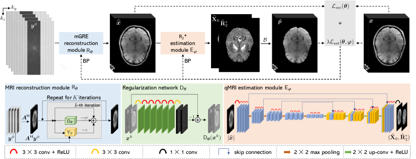
Figure 1: The overview of the CoRRECT framework for training an end-to-end deep network consisting of two modules: ${\mathsf{R}}_{\bm{\theta}}$ for reconstructing mGRE MRI images and ${\mathsf{E}}_{\bm{\varphi}}$ for estimating corresponding $R_{2}^{\ast}$ maps. The network takes input as subsampled, noisy, and motion-corrupted k-space measurements. ${\mathsf{R}}_{\bm{\theta}}$ is implemented as a deep model-based architecture (DMBA) initialized using the zero-filled reconstruction. ${\mathsf{E}}_{\bm{\varphi}}$ is implemented as a customized U-Net architecture mapping the output of ${\mathsf{R}}_{\bm{\theta}}$ to the desired $R_{2}^{\ast}$ map.The whole network is trained end-to-end using fully-sampled mGRE sequence data without any ground-truth quantitative $R_{2}^{\ast}$ maps.

3.2 CoRRECT Architecture

CoRRECT considers a motion-corrupted version of Eq. (1), where the subsampled measurements ${\bm{y}}^{\phi}$ are related to the mGRE image ${\bm{x}}$ with $N$ echo times as

$${\bm{y}}^{\phi}={\bm{A}}\phi({\bm{x}})+{\bm{e}}\;.$$ (8)

Here, the function $\phi$ denotes the effect of the unknown motion of the object during scanning. Our imaging pipeline produces both the motion-corrected mGRE image ${\bm{x}}$ and the corresponding $R_{2}^{\ast}$ map by training a DMBA on a set of ground-truth mGRE images $\{{\bm{x}}_{j}\}_{j=1}^{J}$ and their noisy, motion-corrupted and subsampled measurements $\{{\bm{y}}_{j}^{\phi}\}_{j=1}^{J}$ given the measurement operators $\{{\bm{A}}\}_{j=1}^{J}$ for each acquisition. Fig. 1 summarizes the CoRRECT framework by omitting the sample index $j$ for simplicity.

3.2.1 Motion Simulation

We developed a motion simulation procedure to obtain a training dataset consisting of pairs of ground-truth mGRE images ${\bm{x}}_{j}$ and their subsampled, noisy, and motion-corrupted measurements ${\bm{y}}^{\phi}_{j}$ (see details in Sec.  4.2). The motion-corrupted measurements ${\bm{y}}^{\phi}_{j}$ are simulated by replacing regions of the motion-free k-space data of ${\bm{x}}_{j}$ with its moved version $\phi({\bm{x}}_{j})$. Let the diagonal matrix ${\bm{H}}_{jl}\in\{0,1\}^{m\times m}$ denote a binary map where its diagonal elements have values 1 in locations corrupted by the $l$-th motion event, simulating the beginning and duration of this motion. Then, ${\bm{y}}^{\phi}_{j}$ with a total $L\geq 1$ motion events can be modeled as

$${\bm{y}}^{\phi}_{j}=({\bm{I}}-\sum_{l=1}^{L}{\bm{H}}_{jl}){\bm{A}}_{j}{\bm{x}}_{j}+\sum_{l=1}^{L}{\bm{H}}_{jl}{\bm{A}}_{j}\phi({\bm{x}}_{j})+{\bm{e}}_{j}\;,$$ (9)

where ${\bm{I}}\in\mathbb{R}^{m\times m}$ is an identity matrix. Our model is trained by using ${\bm{x}}_{j}$ as a label for the motion-corrupted input measurement ${\bm{y}}^{\phi}_{j}$, enabling motion-corrected mapping of $R_{2}^{\ast}$.

3.2.2 mGRE Reconstruction Module

The mGRE reconstruction module ${\mathsf{R}}_{\bm{\theta}}$ seeks to produce high-quality $N$-echo mGRE image ${\widehat{\bm{x}}}_{j}$ given the subsampled, noisy, and motion-corrupted k-space measurements ${\bm{y}}^{\phi}_{j}$ and the measurement operator ${\bm{A}}_{j}$

$${\widehat{\bm{x}}}_{j}={\mathsf{R}}_{\bm{\theta}}({\bm{y}}^{\phi}_{j};{\bm{A}}_{j})\;.$$ (10)

This module is a $K$-layer architecture consisting of two types of sub-modules: (a) data-consistency sub-module for ensuring that predicted mGRE images match the k-space measurements; (b) regularization sub-module consisting of a CNN ${\mathsf{D}}_{\bm{\theta}}$ with trainable parameters ${\bm{\theta}}\in\mathbb{R}^{p}$. The data-consistency sub-module is implemented as the gradient-step of the least-squares penalty (4)

$$\nabla g({\bm{x}}_{j})={\bm{A}}_{j}^{\mathsf{H}}({\bm{A}}_{j}{\bm{x}}_{j}-{\bm{y}}_{j}^{\phi})\ ,$$ (11)

where ${\bm{A}}_{j}^{\mathsf{H}}$ denotes the hermitian transpose of the measurement operator ${\bm{A}}_{j}$. As shown in Fig. 1, the reconstruction module is initialized as ${\bm{A}}^{\mathsf{H}}_{j}{\bm{y}}^{\phi}_{j}$. In our implementation, we set $K=8$ and use a customized DnCNN [64] for the implementation of the regularization network ${\mathsf{D}}_{\bm{\theta}}$. Our customized ${\mathsf{D}}_{\bm{\theta}}$ consists of 7 layers, where the first and the last is a convolution (conv) layer followed by rectified linear unit (ReLU), and the middle ones are just convolution layers. Kernel sizes of all convs are set to 3, strides to 1, and number of filters to 64. ${\mathsf{D}}_{\bm{\theta}}$ is implemented using the strategy of residue learning, where its outputs are the artifacts in the inputs, and the clean predictions are obtained by subtracting those artifacts from the inputs. The weights of ${\mathsf{D}}_{\bm{\theta}}$ are shared across all $K$ steps for memory efficiency. To enable the reconstruction for complex mGRE data, the input of ${\mathsf{D}}_{\bm{\theta}}$ are split to 2 channels that consist of the real (denoted as $\operatorname{Re}$) and imaginary (denoted as $\operatorname{Im}$) parts.

3.2.3 $R_{2}^{\ast}$ Estimation Module

The mGRE reconstruction module ${\mathsf{R}}_{\bm{\theta}}$ is followed by a $R_{2}^{\ast}$ estimation module ${\mathsf{E}}_{\bm{\varphi}}$ that produces $R_{2}^{\ast}$ from mGRE images. We implement ${\mathsf{E}}_{\bm{\varphi}}$ using a CNN customized from U-Net [32] with trainable parameters ${\bm{\varphi}}\in\mathbb{R}^{q}$. Our customized U-Net consists of five encoder blocks, four decoder blocks with skip connections, and an output block. For each block in encoder and decoder blocks, it consists of convolutions followed by ReLU. Kernel sizes of all convolutions are set to 3 and strides to 1. The number of filters are set to 64, 128, 256, 512, and 1024 in each encoder block and to 512, 256, 128, and 64 in each decoder block sequentially from inputs to outputs. The network ${\mathsf{E}}_{\bm{\varphi}}$ takes the magnitude of the reconstructed $N$-echo mGRE image ${\widehat{\bm{x}}}_{j}$ from ${\mathsf{R}}_{\bm{\theta}}$ as the input and produces the qMRI maps $(\widehat{{\mathbf{X}}}_{0},\widehat{{\mathbf{R}}}_{2}^{\ast})_{j}$ as the output

$$(\widehat{{\mathbf{X}}}_{0},\widehat{{\mathbf{R}}}_{2}^{\ast})_{j}={\mathsf{E}}_{\bm{\varphi}}(|{\widehat{\bm{x}}}_{j}|)\;,$$ (12)

where $|\cdot|$ returns the magnitude of its input vector, and $\widehat{{\mathbf{X}}}_{0}\in\mathbb{R}^{n},\widehat{{\mathbf{R}}}_{2}^{\ast}\in\mathbb{R}^{n}$ denote the vectorized $X_{0}$ and $R_{2}^{\ast}$ outputs from the estimation module, respectively.

3.3 CoRRECT Training

We adopt a self-supervised learning strategy to train the CoRRECT architecture end-to-end, where only the mGRE images are used for training without any ground-truth $(X_{0},R_{2}^{\ast})$ maps. Consider the intermediate mGRE output ${\widehat{\bm{x}}}_{j}$ produced by ${\mathsf{R}}_{\bm{\theta}}$ in Eq. (10) and the corresponding quantitative map $(\widehat{{\mathbf{X}}}_{0},\widehat{{\mathbf{R}}}_{2}^{\ast})_{j}$ produced by ${\mathsf{E}}_{\bm{\varphi}}$ in Eq. (12). The training is implemented by minimizing two loss functions: the mGRE reconstruction loss $\mathcal{L}_{\mathrm{rec}}({\bm{\theta}})$ and the $R_{2}^{\ast}$ estimation loss $\mathcal{L}_{\mathrm{est}}({\bm{\theta}},{\bm{\varphi}})$. Given data ${\bm{x}}_{j}$ and ${\bm{y}}^{\phi}_{j}$, the mGRE reconstruction loss $\mathcal{L}_{\mathrm{rec}}({\bm{\theta}})_{j}$ measures the difference between the reconstructed mGRE image ${\widehat{\bm{x}}}_{j}$ and the ground truth mGRE image ${\bm{x}}_{j}$ as

$$\mathcal{L}_{\mathrm{rec}}({\bm{\theta}})_{j}=\mathcal{L}({\widehat{\bm{x}}}_{j},{\bm{x}}_{j})\ .$$ (13)

The $R_{2}^{\ast}$ estimation loss $\mathcal{L}_{\mathrm{est}}({\bm{\theta}},{\bm{\varphi}})_{j}$ enforces consistency of the produced mGRE images from the estimated $(X_{0},R_{2}^{\ast})$ maps to the ground-truth mGRE images. The estimation loss uses the biophysical model ${{\bm{\hat{p}}}_{j}={\mathcal{B}}((\widehat{{\mathbf{X}}}_{0},\widehat{{\mathbf{R}}}_{2}^{\ast})_{j};{\bm{f}}_{j})}$ in Eq. (7) to relate the mGRE images and the quantitative $R_{2}^{\ast}$ maps

$$\mathcal{L}_{\mathrm{est}}({\bm{\theta}},{\bm{\varphi}})_{j}=\mathcal{L}(|{\bm{M}}_{j}{\bm{\hat{p}}}_{j}|,|{\bm{M}}_{j}{\bm{x}}_{j}|),$$ (14)

where ${\bm{f}}_{j}\in\mathbb{C}^{n}$ denotes the vectorized $F(t)$ function pre-computed using the VSF approach [63] from ground-truth mGRE data ${\bm{x}}_{j}$ to compensate for the effect of macroscopic magnetic field inhomogeneities, and ${\bm{M}}_{j}$ denotes the voxel-wise region extraction mask (REM) where the biophysical model applies. Note that ${\bm{M}}_{j}$ and $\{{\bm{f}}_{j}\}$ are only needed during training for evaluating the $R_{2}^{\ast}$ estimation loss, but not during the inference. Given losses $\mathcal{L}_{\mathrm{rec}}({\bm{\theta}})_{j}$ and $\mathcal{L}_{\mathrm{est}}({\bm{\theta}},{\bm{\varphi}})_{j}$, CoRRECT training seeks to minimize their combination over a training set consisting of $J$ samples

$${\bm{\theta}}^{\ast},{\bm{\varphi}}^{\ast}=\mathop{\mathrm{arg\,min}}_{{\bm{\theta}},{\bm{\varphi}}}\sum_{j=1}^{J}\left\{\mathcal{L}_{\mathrm{rec}}({\bm{\theta}})_{j}+\lambda\mathcal{L}_{\mathrm{est}}({\bm{\theta}},{\bm{\varphi}})_{j}\right\},$$ (15)

where $\lambda>0$ is a weight parameter. The learned parameters ${\bm{\theta}}^{\ast}$ and ${\bm{\varphi}}^{\ast}$ can be computed by using gradient-based minimization algorithms such as SGD or Adam.

CoRRECT is a self-supervised learning method in the sense that it does not need ground-truth quantitative $R_{2}^{\ast}$ maps during training. Instead, it is trained using only mGRE images and our knowledge of the biophysical model ${\mathcal{B}}$ connecting the mGRE signal with $R_{2}^{\ast}$. The biophysical model accounts for magnetic field inhomogeneities by using $F(t)$, which enables the estimation module ${\mathsf{E}}_{\bm{\varphi}}$ to compensate for macroscopic magnetic field inhomogeneities, thus producing motion-artifact-corrected and $B0$-inhomogeneity-corrected $R_{2}^{\ast}$ maps. Note that $F(t)$ is only required during training not inference, enabling fast end-to-end estimation of quantitative maps. As corroborated by our emirical results, the joint training of ${\mathsf{R}}_{\bm{\theta}}$ and ${\mathsf{E}}_{\bm{\varphi}}$ within CoRRECT leads to better overall performance.

4 Experimental Validation

In this section, we present numerical results on simulated and experimentally collected mGRE data showing the ability of CoRRECT to provide high-quality $R_{2}^{\ast}$ maps from subsampled, noisy, and motion-corrupted k-space measurements.

4.1 Dataset Preparation

We use fully-sampled k-space mGRE data of the brain to generate the synthetic subsampled, noisy, and motion-corrupted measurements. These brain data were collected from 15 healthy volunteers using a Siemens 3T Trio MRI scanner and a 32-channel phased-array head coil. Studies were conducted with the approval of the local IRB of Washington University. All volunteers provided informed consent. The data were obtained using a 3D version of the mGRE sequence with $N=10$ gradient echoes followed by a navigator echo [65] used to reduce artifacts induced by physiological fluctuations during the scan. Sequence parameters were flip angle $FA=30^{\circ}$, voxel size of $1\times 1\times 2$ mm³, first echo time $t_{1}=4$ ms, echo spacing $\Delta t=4$ ms (monopolar readout), repetition time TR $=50$ ms. The dimension of raw measurement for each subject from each coil at a single echo time was $N^{k_{x}}\times N^{k_{y}}\times N^{k_{z}}$ with $k_{x}$ and $k_{y}$ both being the phase-encoding dimension and $k_{z}$ being read-out (frequency-encoding) dimension, respectively. In our data, $N^{k_{x}}=72$, $N^{k_{y}}=192$, and $N^{k_{z}}=256$. Due to limited GPU memory, we convert 3D k-space data into 2D slices by taking a 1D Fourier Transform along the $k_{x}$ dimension and perform 3D MRI reconstruction and $R_{2}^{\ast}$ estimation in a slice-by-slice manner.

The 15 subjects were split into 10, 2, and 3 for training, validation, and testing, respectively. For each subject, we extracted the middle 25 to 56 slices (72 in total) of the brain volume that contain most relevant regions of the brain. This produces 3100 images for training, 620 for validation, and 930 for testing. For each slice, $10$-echo mGRE images of fully-sampled, noise- and motion-free k-space data was used as the ground truth, corresponds to the target image ${\bm{x}}$ in Eq. (8). The ground-truth images ${\bm{x}}$ deformed with the synthetic motion function $\phi$, measured using the forward operator ${\bm{A}}$, and contaminated by AWGN in Eq. (8) to generate artifact-corrupted measurements ${\bm{y}}^{\phi}$ (see Sec. 4.2). The data $\{{\bm{x}}_{j},{\bm{y}}_{j}^{\phi}\}$ of all samples were used for training and quantitative evaluation. Additional experimental data with clearly visible motion artifacts were used for experimentally evaluating the performance of our network. The coil sensitivity maps for each slice were estimated from its $1$st echo of fully sampled k-space data using ESPIRiT [66] for both simulated and experimental data.

Table 1: Quantitative evaluation of CoRRECT on simulated data at different sampling rates. Note how CoRRECT outperforms all the baseline methods in terms of both mGRE reconstruction and $R_{2}^{\ast}$ estimation in terms of SNR and SSIM.

Images	mGRE						$R_{2}^{\ast}$
Metric	SNR (dB)			SSIM			SNR (dB)			SSIM
Acceleration rate	x2	x4	x8	x2	x4	x8	x2	x4	x8	x2	x4	x8
ZF+NLLS	16.72	14.73	14.00	0.90	0.86	0.85	6.70	6.30	6.17	0.85	0.82	0.82
TV	21.46	19.88	17.05	0.81	0.8	0.77	12.21	11.72	10.60	0.92	0.90	0.87
RED	21.49	20.10	17.49	0.92	0.90	0.87	12.16	11.70	10.59	0.91	0.90	0.87
U-Net	20.79	19.25	18.09	0.92	0.90	0.88	12.08	11.39	10.77	0.91	0.89	0.88
DU	21.53	20.36	19.08	0.93	0.91	0.90	12.20	11.79	11.15	0.92	0.90	0.89
CoRRECT (Ours)	22.12	20.66	19.25	0.93	0.91	0.90	12.99	12.33	11.60	0.92	0.90	0.89

4.2 Training Data Simulation

In order to train our architecture, we need matched pairs of clean mGRE images ${\bm{x}}$ and corresponding k-space measurements ${\bm{y}}^{\phi}$. This section discussed our simulation pipeline for generating such training data that accounts for subsampling, noise, and motion artifacts.

4.2.1 Accounting for Object Motion

The motion artifacts in k-space measurements are modeled as a series of physical motions, such as shifts or rotations, that result in the perturbation of blocks of k-space lines. We implement this process by replacing sections of k-space lines of the ground-truth MR images ${\bm{x}}$ with those from their moved versions to synthesize motion artifacts. To generate a wide-range of artifacts, we control the number of movements, the duration of each movement, and the amplitude of each movements as random numbers following the configuration in [60].

4.2.2 Accounting for Subsampling and Noise

The k-space measurements contaminated by simulated motion are further subsampled and contaminated by AWGN. We use a Cartesian sampling pattern that fully-samples along $k_{x}$ and $k_{z}$ dimensions, and subsamples along the $k_{y}$ dimension. We considered three sampling rates $50\%$, $25\%$, and $12.5\%$, which we refer to as acceleration rates $\times 2$, $\times 4$ and $\times 8$, respectively. For each rate, we keep the central 60 out of 192 lines along $k_{y}$. The simulation ${\bm{y}}^{\phi}$ finally includes the addition of AWGN corresponding to an input SNR of 40dB.

4.3 Experimental Setup

We consider the performance of CoRRECT for the reconstruction of mGRE images and estimation of $R_{2}^{\ast}$ maps.

4.3.1 Baseline Methods for mGRE Reconstruction

We consider several well-known algorithms for image reconstruction, including TV [5], U-Net [32], and RED [40]. We also investigate a deep unfodling (DU) network identical to the image reconstruction module of CoRRECT. Inclusion of DU helps to illustrate improvements due to joint training. TV is a traditional optimization-based method that does not require training, while other methods are all DL methods with publicly available implementations. We trained the DL methods on motion-free data to handle mGRE reconstruction. We used the same DnCNN [64] architecture used in our image reconstruction module as the AWGN denoiser for RED. The RED denoisers were trained for AWGN removal at four noise levels corresponding to noise variances $\sigma\in${1, 3, 5, 7}. For each experiment with RED, we selected the denoiser achieving the highest SNR. DU shares the same setting as our image reconstruction module, except that it is not trained using the $R_{2}^{\ast}$ estimation module. We ran TV and RED both for 50 iterations. We fixed the step size $\gamma=0.5$ for TV, RED, DU, and CoRRECT. We used fminbound in the scipy.optimize toolbox to identify the optimal regularization parameters $\tau$ for TV and RED at the inference time, and learned its value through training for DU and CoRRECT.

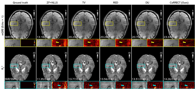
Figure 2: Quantitative and visual evaluation of CoRRECT on simulated data corrupted with synthetic motion, sampled using acceleration factor $\times 4$. The bottom-left corner of each image provides the SNR and SSIM values with respect to the ground-truth. Arrows in the zoomed-in plots highlight brain regions that are well reconstructed using CoRRECT. The $R_{2}^{\ast}$ corresponding to TV, RED, and DU are obtained by the recent LEARN-BIO network [60]. Note the excellent quantitative performance of CoRRECT for mGRE reconstruction and $R_{2}^{\ast}$ estimation.

4.3.2 Baseline Methods for $R_{2}^{\ast}$ Estimation

We applied the DL-based $R_{2}^{\ast}$ estimation method LEARN-BIO [60] to the reconstructed mGRE images from baseline methods to compute the corresponding $R_{2}^{\ast}$ maps as comparisons to the ones from our end-to-end training. LEARN-BIO has the same architecture as ${\mathsf{E}}_{\bm{\varphi}}$ of CoRRECT, except that it is not jointly trained with ${\mathsf{R}}_{\bm{\theta}}$. We trained two LEARN-BIO networks, namely LEARN-BIO (clean) and LEARN-BIO (motion). LEARN-BIO (clean) is trained on motion artifact-free mGRE images and applied to ground-truth mGRE images to get ground-truth $R_{2}^{\ast}$ reference images for quantitative evaluation. LEARN-BIO (motion) is trained on motion-corrupted mGRE images (generated with the same motion simulation configuration introduced in Sec. 4.2) to compute motion-corrected $R_{2}^{\ast}$ maps. We applied this network to all reconstruction methods to see their ability to produce $R_{2}^{\ast}$ maps. As an additional reference, we used the traditional voxel-wise NLLS approach to estimate $R_{2}^{\ast}$ maps from subsampled, noisy, and motion-corrupted mGRE images reconstructed using zero-filling (ZF), denoted as ZF+NLLS. As described in Sec. 3.1, NLLS is a standard iterative fitting method for computing $R_{2}^{\ast}$ based on Eq. (7), where in each iteration, the regression is conducted by combining the data from different echo times $t$ with their $F(t)$ values voxel by voxel. Prior to the NLLS fitting, a brain extraction tool, implemented in the Functional Magnetic Resonance Imaging of the Brain Library (FMRIB), is used to generate REMs to mask out both skull and background voxels in all mGRE data [67], where the signal model defined in Eq. (7) doesn’t apply. NLLS is run over only the set of unmasked voxels. We use the same REMs in the loss function Eq. (14) for training $R_{2}^{\ast}$ estimation module as well as in the baseline LEARN-BIO method. All the results of $R_{2}^{\ast}$ presented in this paper were also masked before visualization.

4.3.3 Implementation Details and Evaluation Metrics

We use the $\ell_{2}$ loss for $\mathcal{L}_{\mathrm{rec}}({\bm{\theta}})$ and $\mathcal{L}_{\mathrm{est}}({\bm{\theta}},{\bm{\varphi}})$ using the weighting parameter $\lambda=1$. We use the Adam [68] optimizer to minimize the loss and set the initial learning rate to $1\times 10^{-5}$. We performed all our experiments on a machine equipped with 8 GeForce RTX 2080 GPUs. For quantitative evaluation, we use signal-to-noise ratio (SNR), measured in dB, and structural similarity index (SSIM), relative to the ground-truth. Since the ground-truth is not available for experimental data, we provide qualitative visual comparisons of different methods.

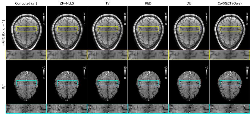
Figure 3: Visual evaluation of CoRRECT on experimentally collected data corrupted with real motion, sampled using acceleration factor $\times 4$. The mGRE image in the first column (denoted with $\times 1$) uses motion-corrupted but fully-sampled k-space data, while the ones in other columns use motion-corrupted and subsampled k-space data. Note the excellent performance of CoRRECT for producing high-quality mGRE and $R_{2}^{\ast}$ images. Note also the abilty of CoRRECT trained on synthetic motion to address artifacts due to real object motion.

4.4 Results on Simulated Data

We first test the performance of CoRRECT on simulated data with synthetic motion corruptions. We followed the configuration in Sec. 4.2 to add random motion to each data slice in our testing dataset to cover comprehensive motion levels. Table 1 summarizes quantitative results of all evaluated methods at different acceleration rates. As highlighted in Table 1, CoRRECT achieves the highest SNR and SSIM values compared to other methods over all considered configurations.

Fig. 2 shows the performance of CoRRECT compared with different baseline methods on exemplar simulated data. The $1$st echo of a complex-valued mGRE image sequence is shown as its normalized magnitude, where the normalization is done by dividing by the mean of the intensity in the $1$st echo of the mGRE sequence. The result of ZF+NLLS shows that subsampling and motion can severely degrade the quality of mGRE images by causing a significant amount of blurring and aliasing artifacts, and consequently leads to suboptimal $R_{2}^{\ast}$ estimation. Baseline methods TV and RED alleviate some of the artifacts in the corrupted image. However, due to their inability to capture the motion effects missed in the forward operator, a considerable amount of artifacts are still observed in mGRE reconstruction. Meanwhile, due to the existence of unknown motion, the forward operator ${\bm{A}}$ that only models the subsampling is no longer accurate and consequently misleads the reconstruction. DU can further reduce the overall artifacts by using a CNN prior to compensate for artifacts through end-to-end training, but is still suboptimal, showing visible artifacts in mGRE reconstruction. As for $R_{2}^{\ast}$ estimation, although a significant improvement over the NLLS fitting is observed by using motion-correction-enabled LEARN-BIO on artifact-contaminated mGRE images from those baseline methods, the estimation still suffers from inaccuracy in the regions indicated by blue arrows. Our proposed method, CoRRECT, managed to achieve the best performance compared to all evaluated baseline methods in terms of sharpness, contrast, artifact removal and accuracy, thanks to joint training of mGRE reconstruction and $R_{2}^{\ast}$ estimation.

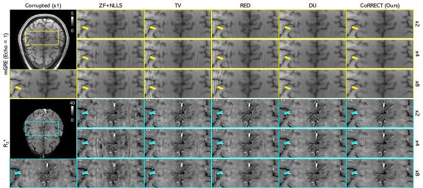
Figure 4: Visual evaluation of CoRRECT on experimentally-collected data corrupted with real motion, subsampled using acceleration rates $\{\times 2,\times 4,\times 8\}$. Arrows in the zoomed-in plots highlight brain regions that are well reconstructed using CoRRECT. Corrupted ($\times 1$) uses motion-corrupted but fully-sampled measurements, while ZF+NLLS, TV, RED, DU and CoRRECT use motion-corrupted and subsampled measurements. Note the improvements due to CoRRECT across different sampling rates.

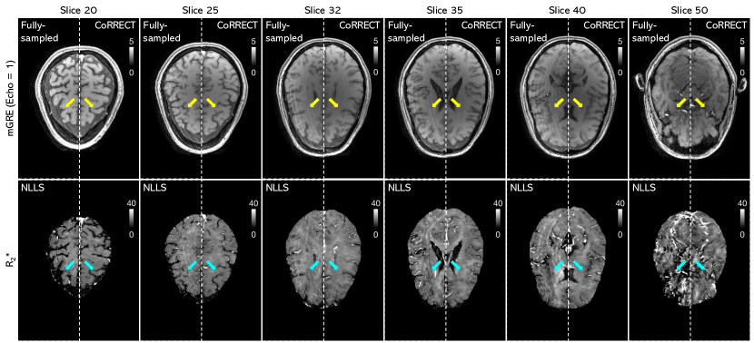
Figure 5: Visual evaluation of CoRRECT on experimental data corrupted with real motion, sampled using acceleration rate $\times 4$. The first row shows several slices of reconstructed mGRE images from the whole brain volume of 72 slices, while the second row shows the corresponding estimated $R_{2}^{\ast}$ maps. In each column of the first row, the images to the left of the dashed line are the mGRE images reconstructed from the fully-sampled, noisy, and motion-corrupted measurements, while the images to the right are the result of the CoRRECT reconstruction from subsampled, noisy, and motion-corrupted measurements. In each column of the second row, the $R_{2}^{\ast}$ maps to the left of the dashed line are estimated using NLLS on mGRE images in the first row, while those to the right are produced by CoRRECT. Arrows in the plots highlight brain regions that are well reconstructed using CoRRECT. Note how CoRRECT can remove artifacts across the whole brain volume.

4.5 Results on Experimental Data

We further validate the performance of our network trained on simulated data using experimental data with real motion corruptions.

Fig. 3 shows the performance of CoRRECT compared to different baseline methods on exemplar experimental data corrupted with real motion and subsampled with acceleration rate $\times 4$. Note that the corrupted mGRE image in the first column, denoted with acceleration rate $\times 1$, corresponds to the corrupted mGRE image of motion-affected but fully-sampled k-space data. The corresponding $R_{2}^{\ast}$, which is estimated using LEARN-BIO (clean), consequently suffers from these motion corruptions as well. While such motion artifacts in this experimental data might not follow our simulation model, we do observe similar results to our synthetic experiments. It can be seen that CoRRECT outperforms the evaluated baseline methods in both mGRE reconstruction and $R_{2}^{\ast}$ estimation in terms of removing artifacts and maintaining sharpness. This shows CoRRECT is capable of handling real motion artifacts while still keeping detailed structural information. Fig. 4 shows comprehensive results across different acceleration rates for the same data sample, where consistently outstanding and robust performance of CoRRECT is observed.

Fig. 5 further demonstrates the performance of our method across different data slices in a whole brain volume, where each slice, in principle, is corrupted with different and random motions during the scan. For each slice, we show the side-to-side comparison between the results of CoRRECT on the subsampled (with acceleration rate $\times 4$), noisy and motion-corrupted measurements and the images obtained from fully-sampled, noisy, and motion-corrupted k-space measurements and their NLLS-estimated $R_{2}^{\ast}$ maps. Note that CoRRECT using subsampled measurements successfully removes the motion artifacts visible in the fully-sampled images. The constant success of CoRRECT on different brain slices proves that our network can work on the whole spectrum of brain volume, highlighting the effectiveness and adaptability of our method.

5 Discussion and Conclusion

This work introduces CoRRECT as a framework for estimating $R_{2}^{\ast}$ maps from subsampled, noisy, and artifact-corrupted mGRE k-space measurements. Unlike existing DL techniques for MRI that separate quantitative parameter estimation from image reconstruction, CoRRECT addresses both tasks by integrating three core components: (a) an end-to-end model-based neural network, (b) a training scheme accounting for motion-artifacts, and (c) a loss function for training without ground-truth $R_{2}^{*}$ maps. Our extensive validation corroborate the potential of DMBAs integrating multiple models to produce high-quality images from noisy, subsampled, and artifact-corrupted measurements.

References

- [1] M. Lustig, D. L. Donoho, and J. M. Pauly, “Sparse MRI: The application of compressed sensing for rapid MR imaging,” Magn. Reson. Med., vol. 58, no. 6, pp. 1182–1195, Dec. 2007.
- [2] A. Danielyan, V. Katkovnik, and K. Egiazarian, “BM3D frames and variational image deblurring,” IEEE Trans. Image Process., vol. 21, no. 4, pp. 1715–1728, Apr. 2012.
- [3] M. Elad and M. Aharon, “Image denoising via sparse and redundant representations over learned dictionaries,” IEEE Trans. Image Process., vol. 15, no. 12, pp. 3736–3745, Dec. 2006.
- [4] Y. Hu, S. G. Lingala, and M. Jacob, “A fast majorize-minimize algorithm for the recovery of sparse and low-rank matrices,” IEEE Trans. Image Process., vol. 21, no. 2, pp. 742–753, Feb. 2012.
- [5] L. I. Rudin, S. Osher, and E. Fatemi, “Nonlinear total variation based noise removal algorithms,” Physica D, vol. 60, no. 1–4, pp. 259–268, Nov. 1992.
- [6] F. Knoll, K. Hammernik, C. Zhang, S. Moeller, T. Pock, D. K. Sodickson, and M. Akcakaya, “Deep-learning methods for parallel magnetic resonance imaging reconstruction: A survey of the current approaches, trends, and issues,” IEEE Signal Process. Mag., vol. 37, no. 1, pp. 128–140, Jan. 2020.
- [7] A. Lucas, M. Iliadis, R. Molina, and A. K. Katsaggelos, “Using deep neural networks for inverse problems in imaging: Beyond analytical methods,” IEEE Signal Process. Mag., vol. 35, no. 1, pp. 20–36, Jan. 2018.
- [8] M. T. McCann, K. H. Jin, and M. Unser, “Convolutional neural networks for inverse problems in imaging: A review,” IEEE Signal Process. Mag., vol. 34, no. 6, pp. 85–95, 2017.
- [9] G. Ongie, A. Jalal, C. A. Metzler, R. G. Baraniuk, A. G. Dimakis, and R. Willett, “Deep learning techniques for inverse problems in imaging,” IEEE J. Sel. Areas Inf. Theory, vol. 1, no. 1, pp. 39–56, 2020.
- [10] G. Wang, J. C. Ye, and B. De Man, “Deep learning for tomographic image reconstruction,” Nat. Mach. Intell., vol. 2, no. 12, pp. 737–748, 2020.
- [11] J. Zhang and B. Ghanem, “ISTA-Net: Interpretable optimization-inspired deep network for image compressive sensing,” in 2018 IEEE/CVF Conference on Computer Vision and Pattern Recognition, Jun. 2018, pp. 1828–1837.
- [12] A. Hauptmann, F. Lucka, M. Betcke, N. Huynh, J. Adler, B. Cox, P. Beard, S. Ourselin, and S. Arridge, “Model-based learning for accelerated, limited-view 3-D photoacoustic tomography,” IEEE Trans. Med. Imag., vol. 37, no. 6, pp. 1382–1393, 2018.
- [13] J. Adler and O. Öktem, “Learned primal-dual reconstruction,” IEEE Trans. Med. Imag., vol. 37, no. 6, pp. 1322–1332, Jun. 2018.
- [14] H. K. Aggarwal, M. P. Mani, and M. Jacob, “MoDL: Model-based deep learning architecture for inverse problems,” IEEE Trans. Med. Imag., vol. 38, no. 2, pp. 394–405, Feb. 2019.
- [15] S. A. Hosseini, B. Yaman, S. Moeller, M. Hong, and M. Akcakaya, “Dense recurrent neural networks for accelerated MRI: History-Cognizant unrolling of optimization algorithms,” IEEE J. Sel. Topics Signal Process., vol. 14, no. 6, pp. 1280–1291, Oct. 2020.
- [16] B. Yaman, S. A. H. Hosseini, S. Moeller, J. Ellermann, K. Uğurbil, and M. Akçakaya, “Self-supervised learning of physics-guided reconstruction neural networks without fully sampled reference data,” Magn Reson Med, Jul. 2020.
- [17] S. Mukherjee, M. Carioni, O. Öktem, and C.-B. Schönlieb, “End-to-end reconstruction meets data-driven regularization for inverse problems,” in Advances in Neural Information Processing Systems, vol. 34. Curran Associates, Inc., 2021, pp. 21 413–21 425.
- [18] D. Hernando, K. K. Vigen, A. Shimakawa, and S. B. Reeder, “R2* mapping in the presence of macroscopic B0 field variations,” Magn Reson Med, vol. 68, no. 3, pp. 830–840, Sep. 2012.
- [19] Y. Zhao, J. Wen, A. H. Cross, and D. A. Yablonskiy, “On the relationship between cellular and hemodynamic properties of the human brain cortex throughout adult lifespan,” Neuroimage, vol. 133, pp. 417–429, Jun. 2016.
- [20] X. Ulrich and D. A. Yablonskiy, “Separation of cellular and BOLD contributions to T2* signal relaxation,” Magn Reson Med, vol. 75, no. 2, pp. 606–615, Feb. 2016.
- [21] Y. Zhao, M. E. Raichle, J. Wen, T. L. Benzinger, A. M. Fagan, J. Hassenstab, A. G. Vlassenko, J. Luo, N. J. Cairns, J. J. Christensen, J. C. Morris, and D. A. Yablonskiy, “In vivo Detection of Microstructural Correlates of Brain Pathology in Preclinical and Early Alzheimer Disease with Magnetic Resonance Imaging,” Neuroimage, vol. 148, pp. 296–304, Mar. 2017.
- [22] J. Wen, M. S. Goyal, S. V. Astafiev, M. E. Raichle, and D. A. Yablonskiy, “Genetically defined cellular correlates of the baseline brain MRI signal,” PNAS, vol. 115, no. 41, pp. E9727–E9736, Oct. 2018.
- [23] B. Xiang, W. Jie, R. Schmidt, D. Yablonskiy, and A. Cross, “Quantitative assessment of multiple sclerosis tissue damage and partial repair in a biopsy proven demyelinating brain lesion using gradient recalled echo imaging,” in Multiple Sclerosis Journal, vol. 26. London, England: SAGE PUBLICATIONS LTD 1 OLIVERS YARD, 55 CITY ROAD, LONDON EC1Y 1SP, ENGLAND, May 2020, pp. 93–94.
- [24] S. V. V. N. Kothapalli, T. L. Benzinger, A. J. Aschenbrenner, R. J. Perrin, C. F. Hildebolt, M. S. Goyal, A. M. Fagan, M. E. Raichle, J. C. Morris, and D. A. Yablonskiy, “Quantitative Gradient Echo MRI Identifies Dark Matter as a New Imaging Biomarker of Neurodegeneration that Precedes Tissue Atrophy in Early Alzheimer Disease,” p. 2021.04.27.21256098, Apr. 2021.
- [25] N. T. Roberts, L. A. Hinshaw, T. J. Colgan, T. Ii, D. Hernando, and S. B. Reeder, “B0 and B1 inhomogeneities in the liver at 1.5 T and 3.0 T,” Magn Reson Med, vol. 85, no. 4, pp. 2212–2220, 2021.
- [26] M. V. W. Zibetti, P. M. Johnson, A. Sharafi, K. Hammernik, F. Knoll, and R. R. Regatte, “Rapid mono and biexponential 3D-T1 mapping of knee cartilage using variational networks,” Sci Rep, vol. 10, p. 19144, Nov. 2020.
- [27] Y. Gao, M. Cloos, F. Liu, S. Crozier, G. B. Pike, and H. Sun, “Accelerating quantitative susceptibility and R2* mapping using incoherent undersampling and deep neural network reconstruction,” NeuroImage, vol. 240, p. 118404, Oct. 2021.
- [28] Y. Wu, Y. Ma, J. Du, and L. Xing, “Accelerating quantitative MR imaging with the incorporation of B1 compensation using deep learning,” Magnetic Resonance Imaging, vol. 72, pp. 78–86, Oct. 2020.
- [29] J. A. Fessler, “Optimization methods for magnetic resonance image reconstruction,” IEEE Signal Process. Mag., vol. 1, no. 37, pp. 33–40, Jan. 2020.
- [30] A. S. Lundervold and A. Lundervold, “An overview of deep learning in medical imaging focusing on MRI,” Zeitschrift für Medizinische Physik, vol. 29, no. 2, pp. 102–127, May 2019.
- [31] G. Zeng, Y. Guo, J. Zhan, Z. Wang, Z. Lai, X. Du, X. Qu, and D. Guo, “A review on deep learning MRI reconstruction without fully sampled k-space,” BMC Medical Imaging, vol. 21, no. 1, p. 195, Dec. 2021.
- [32] O. Ronneberger, P. Fischer, and T. Brox, “U-Net: Convolutional networks for biomedical image segmentation,” in Medical Image Computing and Computer-Assisted Intervention (MICCAI), Munich, Germany, Oct. 2015, pp. 234–241.
- [33] S. Wang, Z. Su, L. Ying, X. Peng, S. Zhu, F. Liang, D. Feng, and D. Liang, “Accelerating magnetic resonance imaging via deep learning,” in Proc. Int. Symp. Biomedical Imaging, Apr. 2016, pp. 514–517.
- [34] Y. S. Han, J. Yoo, and J. C. Ye, “Deep learning with domain adaptation for accelerated projection reconstruction MR,” Magn Reson Med, vol. 80, no. 3, pp. 1189–1205, Sep. 2017.
- [35] J. Schlemper, J. Caballero, J. V. Hajnal, A. N. Price, and D. Rueckert, “A deep cascade of convolutional neural networks for dynamic MR image reconstruction,” IEEE Trans. Med. Imag., vol. 37, no. 2, pp. 491–503, Feb. 2018.
- [36] S. V. Venkatakrishnan, C. A. Bouman, and B. Wohlberg, “Plug-and-play priors for model based reconstruction,” in Proc. IEEE Global Conf. Signal Process. and Inf. Process., Austin, TX, USA, Dec. 2013, pp. 945–948.
- [37] S. Sreehari, S. V. Venkatakrishnan, B. Wohlberg, G. T. Buzzard, L. F. Drummy, J. P. Simmons, and C. A. Bouman, “Plug-and-play priors for bright field electron tomography and sparse interpolation,” IEEE Trans. Comput. Imaging, vol. 2, no. 4, pp. 408–423, Dec. 2016.
- [38] R. Ahmad, C. A. Bouman, G. T. Buzzard, S. Chan, S. Liu, E. T. Reehorst, and P. Schniter, “Plug-and-play methods for magnetic resonance imaging: Using denoisers for image recovery,” IEEE Signal Process. Mag., vol. 37, no. 1, pp. 105–116, 2020.
- [39] U. S. Kamilov, C. A. Bouman, G. T. Buzzard, and B. Wohlberg, “Plug-and-play methods for integrating physical and learned models in computational imaging,” IEEE Signal Process. Mag., 2022, arXiv:2203.17061.
- [40] Y. Romano, M. Elad, and P. Milanfar, “The little engine that could: Regularization by denoising (RED),” SIAM J. Imaging Sci., vol. 10, no. 4, pp. 1804–1844, 2017.
- [41] K. Zhang, W. Zuo, S. Gu, and L. Zhang, “Learning deep CNN denoiser prior for image restoration,” in Proc. IEEE Conf. Computer Vision and Pattern Recognition, Jul. 2017, pp. 3929–3938.
- [42] K. Zhang, W. Zuo, and L. Zhang, “Deep plug-and-play super-resolution for arbitrary blur kernels,” in Proceedings of the IEEE Conference on Computer Vision and Pattern Recognition, Long Beach, CA, USA, 2019, pp. 1671–1681.
- [43] S. H. Chan, X. Wang, and O. A. Elgendy, “Plug-and-play ADMM for image restoration: Fixed-point convergence and applications,” IEEE Trans. Comput. Imag., vol. 3, no. 1, pp. 84–98, 2016.
- [44] E. K. Ryu, J. Liu, S. Wang, X. Chen, Z. Wang, and W. Yin, “Plug-and-play methods provably converge with properly trained denoisers,” in Proc. 36th Int. Conf. Machine Learning (ICML), vol. 97, Long Beach, CA, USA, Jun. 2019, pp. 5546–5557.
- [45] X. Xu, Y. Sun, J. Liu, B. Wohlberg, and U. S. Kamilov, “Provable convergence of plug-and-play priors with MMSE denoisers,” IEEE Signal Process. Lett., vol. 27, pp. 1280–1284, 2020.
- [46] Y. Sun, Z. Wu, X. Xu, B. Wohlberg, and U. S. Kamilov, “Scalable Plug-and-Play ADMM With Convergence Guarantees,” IEEE Trans. Comput. Imaging, vol. 7, pp. 849–863, 2021.
- [47] Y. Yang, J. Sun, H. Li, and Z. Xu, “Deep ADMM-Net for compressive sensing MRI,” in Advances in Neural Information Processing Systems 29, 2016, pp. 10–18.
- [48] F. Liu, “Improving Quantitative Magnetic Resonance Imaging Using Deep Learning,” Semin Musculoskelet Radiol, vol. 24, no. 4, pp. 451–459, Aug. 2020.
- [49] W. Jung, S. Bollmann, and J. Lee, “Overview of quantitative susceptibility mapping using deep learning: Current status, challenges and opportunities,” NMR Biomed., vol. 35, no. 4, p. e4292, 2022.
- [50] L. Feng, D. Ma, and F. Liu, “Rapid MR relaxometry using deep learning: An overview of current techniques and emerging trends,” NMR Biomed, vol. 35, no. 4, p. e4416, Apr. 2022.
- [51] C. Cai, C. Wang, Y. Zeng, S. Cai, D. Liang, Y. Wu, Z. Chen, X. Ding, and J. Zhong, “Single-shot T2 mapping using overlapping-echo detachment planar imaging and a deep convolutional neural network,” Magn Reson Med, vol. 80, no. 5, pp. 2202–2214, Nov. 2018.
- [52] J. Yoon, E. Gong, I. Chatnuntawech, B. Bilgic, J. Lee, W. Jung, J. Ko, H. Jung, K. Setsompop, G. Zaharchuk, E. Y. Kim, J. Pauly, and J. Lee, “Quantitative susceptibility mapping using deep neural network: QSMnet,” NeuroImage, vol. 179, pp. 199–206, Oct. 2018.
- [53] S. Bollmann, K. G. B. Rasmussen, M. Kristensen, R. G. Blendal, L. R. Østergaard, M. Plocharski, K. O’Brien, C. Langkammer, A. Janke, and M. Barth, “DeepQSM - using deep learning to solve the dipole inversion for quantitative susceptibility mapping,” NeuroImage, vol. 195, pp. 373–383, Jul. 2019.
- [54] H. Li, M. Yang, J. Kim, R. Liu, C. Zhang, P. Huang, S. K. Gaire, D. Liang, X. Li, and L. Ying, “Ultra-fast simultaneous T1rho and T2 mapping using deep learning,” in ISMRM Annual Meeting, 2020.
- [55] S. Kahali, S. V. Kothapalli, X. Xu, U. S. Kamilov, and D. A. Yablonskiy, “Deep-learning-based accelerated and noise-suppressed estimation (DANSE) of quantitative gradient recalled echo (qGRE) MRI metrics associated with human brain neuronal structure and hemodynamic properties,” bioRxiv, 2021.
- [56] A. Panda, B. B. Mehta, S. Coppo, Y. Jiang, D. Ma, N. Seiberlich, M. A. Griswold, and V. Gulani, “Magnetic Resonance Fingerprinting-An Overview,” Curr Opin Biomed Eng, vol. 3, pp. 56–66, Sep. 2017.
- [57] O. Cohen, B. Zhu, and M. S. Rosen, “MR fingerprinting Deep RecOnstruction NEtwork (DRONE),” Magn Reson Med, vol. 80, no. 3, pp. 885–894, Sep. 2018.
- [58] Z. Fang, Y. Chen, M. Liu, L. Xiang, Q. Zhang, Q. Wang, W. Lin, and D. Shen, “Deep Learning for Fast and Spatially Constrained Tissue Quantification From Highly Accelerated Data in Magnetic Resonance Fingerprinting,” IEEE Trans Med Imaging, vol. 38, no. 10, pp. 2364–2374, Oct. 2019.
- [59] M. Torop, S. V. V. N. Kothapalli, Y. Sun, J. Liu, S. Kahali, D. A. Yablonskiy, and U. S. Kamilov, “Deep learning using a biophysical model for robust and accelerated reconstruction of quantitative, artifact-free and denoised R2* images,” Magn Reson Med, vol. 84, no. 6, pp. 2932–2942, Dec. 2020.
- [60] X. Xu, S. V. V. N. Kothapalli, J. Liu, S. Kahali, W. Gan, D. A. Yablonskiy, and U. S. Kamilov, “Learning-based motion artifact removal networks for quantitative R2∗ mapping,” Magn. Reson. Med., vol. 88, no. 1, pp. 106–119, 2022.
- [61] H. Jeelani, Y. Yang, R. Zhou, C. M. Kramer, M. Salerno, and D. S. Weller, “A Myocardial T1-Mapping Framework with Recurrent and U-Net Convolutional Neural Networks,” in 2020 IEEE 17th International Symposium on Biomedical Imaging (ISBI), Apr. 2020, pp. 1941–1944.
- [62] D. A. Yablonskiy, “Quantitation of intrinsic magnetic susceptibility-related effects in a tissue matrix. Phantom study,” Magn Reson Med, vol. 39, no. 3, pp. 417–428, Mar. 1998.
- [63] D. A. Yablonskiy, A. L. Sukstanskii, J. Luo, and X. Wang, “Voxel spread function method for correction of magnetic field inhomogeneity effects in quantitative gradient-echo-based MRI,” Magn Reson Med, vol. 70, no. 5, pp. 1283–1292, Nov. 2013.
- [64] K. Zhang, W. Zuo, Y. Chen, D. Meng, and L. Zhang, “Beyond a Gaussian denoiser: Residual learning of deep CNN for image denoising,” IEEE Trans. Image Process, vol. 26, no. 7, pp. 3142–3155, Jul. 2017.
- [65] J. Wen, A. H. Cross, and D. A. Yablonskiy, “On the role of physiological fluctuations in quantitative gradient echo MRI – implications for GEPCI, QSM and SWI,” Magn Reson Med, vol. 73, no. 1, pp. 195–203, Jan. 2015.
- [66] M. Uecker, P. Lai, M. J. Murphy, P. Virtue, M. Elad, J. M. Pauly, S. S. Vasanawala, and M. Lustig, “ESPIRiT — An Eigenvalue Approach to Autocalibrating Parallel MRI: Where SENSE meets GRAPPA,” Magn Reson Med, vol. 71, no. 3, pp. 990–1001, Mar. 2014.
- [67] M. Jenkinson, M. Pechaud, and S. Smith, “BET2: MR-based estimation of brain, skull and scalp surfaces,” in Eleventh Annual Meeting of the Organization for Human Brain Mapping, vol. 17, Toronto, Ontario, Canada, Jun. 2005, p. 167.
- [68] D. Kingma and J. Ba, “Adam: A method for stochastic optimization,” in International Conference on Learning Representations (ICLR), San Diego, CA, USA, May 2015, pp. 1–13.